Article

Quantifying Three-Dimensional Street Network Orientation Entropy in Chongqing, China: Implications for Urban Spatial Order and Environmental Perception

1
College of Civil Engineering and Architecture, Zhejiang University, 866 Yuhangtang Road, Hangzhou 310058, China
2
ZJU-STEC Urban Development and Planning Innovation Joint Research Center, Zhejiang University, 866 Yuhangtang Road, Hangzhou 310058, China
*
Author to whom correspondence should be addressed.
Buildings 2025, 15(14), 2460; https://doi.org/10.3390/buildings15142460
Submission received: 24 May 2025 / Revised: 1 July 2025 / Accepted: 8 July 2025 / Published: 14 July 2025
(This article belongs to the Special Issue Urban Wellbeing: The Impact of Spatial Parameters—2nd Edition)

Abstract

Orientation entropy serves as a critical metric for assessing the directional disorder of urban street networks. However, conventional two-dimensional (2D) approaches neglect vertical variations, limiting their applicability in cities with complex terrains. This study proposes a three-dimensional (3D) orientation entropy framework by integrating elevation data, providing a more comprehensive assessment of urban spatial complexity. We developed a computational workflow combining ArcGIS 10.8 for spatial data extraction and Python 3.10.10 for entropy calculation. A case study in Chongqing, China, explores the relationship between 3D orientation entropy and residents’ perceptions of spatial disorder through a small-scale survey. Although no statistically significant correlation was observed, the findings suggest emerging patterns and underscore the necessity of multidimensional frameworks in evaluating urban spatial experience. This research contributes a novel metric to urban design assessment, particularly in topographically diverse environments, and offers a foundation for future empirical studies.

1. Introduction

1.1. Background and Motivation

With the growing global emphasis on sustainable urban development and livability, understanding and quantifying urban spatial order has become increasingly crucial. Among various spatial attributes, the orientation of urban street networks is closely associated with navigability, accessibility, and perceptual clarity. Spatial order plays a key role in shaping people’s spatial behavior and environmental perception, particularly in topographically complex or three-dimensional urban settings [1,2,3]. The study of spatial networks provides a fundamental theoretical framework to understand such urban structures and their complex interactions across scales [4].
In this context, entropy, a concept from information theory, is used to quantify the degree of disorder. Information entropy, proposed by Shannon in 1948, measures the amount of information [5]. For any random variable X, the greater the uncertainty, the higher the entropy H, and the greater the amount of information required to fully understand it.
Previous researchers applied information entropy to quantify the degree of disorder in the distribution of urban street network orientations, introducing the concept of street orientation entropy. Specifically, the horizontal plane is divided into several equally sized regions through the origin, with each region treated as a random variable X in the context of information entropy [1,6]. Using the city’s street map, directional vectors of the streets are obtained, and the probabilities of these vectors falling into different regions are calculated as the probabilities P(X) of the random variable X. Finally, by substituting the probabilities P(X) into the information entropy formula, the orientation entropy of the streets is calculated, quantifying the degree of directional disorder within the given range [1,5,7,8].
However, urban environments are inherently three-dimensional. Existing studies have demonstrated that 3D visibility and spatial orientation play critical roles in how people perceive and navigate cities. Recent advances in computational urban modeling have introduced various techniques to analyze three-dimensional spatial perception, including the following:
  • Ray-casting algorithms (Turner et al., 2001) [9], which simulate the openness and obstructions from a given viewpoint, providing detailed insights into visual accessibility and perceptual clarity;
  • Voxel-based visibility analysis (Aleksandrov et al., 2019) [10], which discretizes space into three-dimensional units to evaluate visibility probabilities, making it particularly suitable for analyzing complex architectural and urban forms;
  • Space syntax theory, originally developed by Hillier and Hanson (1984) [11], models spatial cognition through network structures such as axial maps and convex spaces. Although initially focused on two-dimensional analysis, recent studies (e.g., Stamps, 2010) [12] have extended its application to 3D environments, enabling a deeper understanding of spatial structures in multi-level and vertical urban settings.
Furthermore, studies integrating voxel-based spatial analysis with syntactic principles have strengthened the understanding of the relationship between spatial morphology and perceptual cognition in three-dimensional urban environments [9,10]. These approaches highlight the necessity of analytical frameworks that capture the complexity of urban spatial perception beyond two-dimensional representations.
Beyond methodological advancements, spatial orientation entropy is closely related to sustainable development goals (SDGs). Urban directionality influences the coherence of movement networks, thereby affecting walkability, green mobility, and environmental comfort. The morphology and circuity of street networks critically shape how navigable and accessible urban environments are perceived [6,7,13,14]. Spatial order has been shown to enhance urban livability and transportation efficiency, while higher directional entropy often reflects disorganized environments that may reduce legibility and navigation ease [6,15].
Recent urban studies emphasize the importance of spatial dimensions within sustainable development frameworks. For example, Manioudis and Meramveliotakis (2022) and Klarin (2018) highlight the role of spatial configuration and urban planning in fostering sustainable urban futures [16,17], although these studies do not explicitly focus on spatial order as defined in this research. Their findings provide a relevant context that complements this study’s approach, which aims to quantify three-dimensional spatial order through orientation entropy, offering a more precise and operational metric to support sustainability objectives. Thus, this study situates itself at the intersection of spatial order analysis and sustainability research.
Building upon prior research, this study proposes a novel three-dimensional street orientation entropy metric that integrates 3D geometry into entropy-based spatial analysis. The mathematical and geometrical principles underlying urban morphogenesis provide essential insights into the development of such spatial metrics [18]. This approach extends traditional two-dimensional spatial metrics by incorporating the vertical structure of street networks, enhancing the modeling of perceptual complexity and spatial coherence. Ultimately, it contributes both to the theoretical development of 3D urban morphology and to the practical assessment of spatial quality for livable and sustainable city design.

1.2. Limitation of Previous Research

In the aforementioned method, the random variable X is defined by equally dividing the horizontal plane, and then the street map is used to obtain street directional vectors for statistical analysis of the probability of X’s occurrence. The result reflects the degree of disorder in the horizontal distribution of streets, specifically the two-dimensional orientation entropy of streets, without considering variations in the vertical direction. This definition makes the indicator particularly unsuitable for regions with significant terrain variations, such as mountainous areas and hills, where the vertical directional component cannot be ignored, which restricts the applicability of the indicator [1,19]. Additionally, the assumption of planarity in traditional street network representations may overlook complex multi-level structures present in urban morphology, affecting analytical accuracy [20].
To address these limitations, this study introduces the concept of three-dimensional orientation entropy of streets, aimed at quantifying the degree of disorder in the distribution of urban street network orientations in three-dimensional space. The extension of street orientation entropy aims to increase its applicability, with the goal of having it more widely used as a quantitative indicator in future urban design evaluations.
Results indicate that 3D orientation entropy values are consistently higher than their 2D counterparts, reflecting a more nuanced and accurate representation of directional disorder in topographically complex areas. Spatial distribution maps (to be supplemented) illustrate notable differences between the two metrics, with the 3D approach revealing finer spatial variations in orientation. This quantitative comparison validates the enhanced capability of 3D orientation entropy to characterize complex spatial structures and perceptual differences in urban environments, highlighting the methodological innovation and practical significance of the proposed approach.

2. Definition

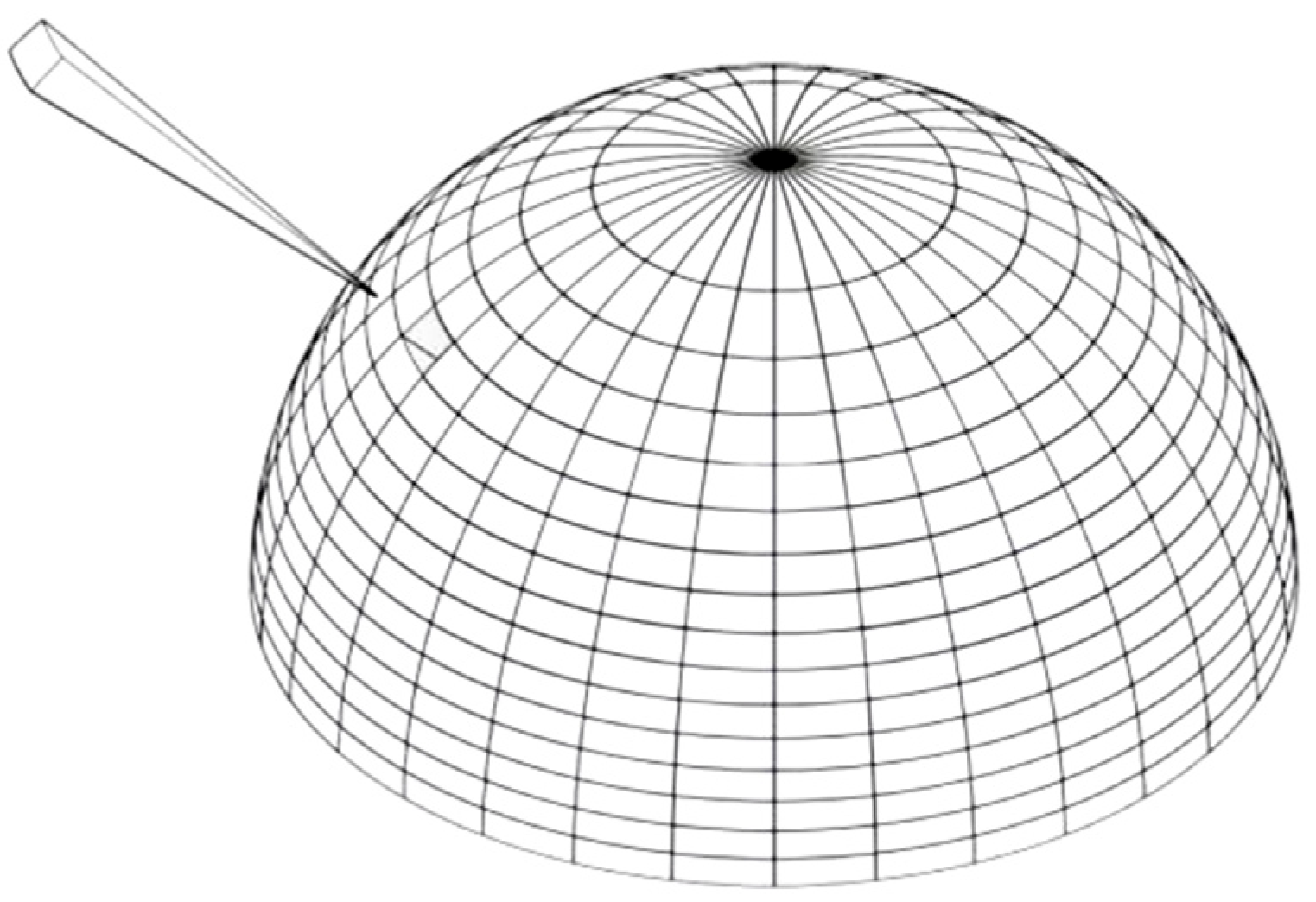
2.1. Three-Dimensional Orientation Entropy: Concept and Spatial Partitioning

Distinct from two-dimensional orientation entropy, three-dimensional orientation entropy requires the division of three-dimensional space into uniform partitions [1]. These partitioned spatial units are treated as the random variable X in the context of information entropy [5]. The probability of the occurrence of street direction vectors within each spatial unit is statistically determined and subsequently accumulated according to the formula (Equation (1)) to derive the result.
H(X) = −∑ P(x) · log2[P(x)]
Assuming all roads are bidirectional, each road will have two opposite direction vectors. Only the vector located on the upper hemisphere is selected as the road direction vector. Thus, the unit vectors of road direction vectors collectively form a unit hemisphere with the origin as the center in three-dimensional space [18].
First, the hemisphere is divided into 32 sections by passing through the center of the sphere along the positive Z-axis and creating divisions every π/16. These sections are sequentially numbered from 1 to 32 based on their azimuth angles.
Next, planes are made parallel to the base of the hemisphere at intervals of 1/16, further subdividing the hemisphere based on polar angles, sequentially numbered from 1 to 16. This process results in a total of 512 sections. The spatial ranges defined by the contraction of these 512 spherical sections towards the center of the sphere are of equal volume, and these are defined as the random variable X (Figure 1) [18].
Each spatial unit is assigned a unit number (32i + j), where i is the azimuthal angle range index and j is the polar angle range index (Equation (2)).
azimuthal angle φ ∈ [(π/16)·(I − 1), (π/16)·i],   i = 1, 2, 3, …, 15, 16
polar angle θ ∈ [arccos((j − 1)/16), arccos(j/16)],   j = 1, 2, 3, …, 15, 16
The result is a set of spatial units with equal volume passing through the origin, which can be verified using the volume formula for solids of revolution in calculus [21].
According to the properties of information entropy, the range of entropy values is [0, log2(t)]: the minimum value of 0 occurs when the probability distribution of the random variable is fixed, while the maximum value of log2(t) occurs when the probability distribution is uniform, where t represents the number of the random variable X. Thus, when the directional vectors of streets are concentrated within a single spatial unit, the three-dimensional orientation entropy value is at its minimum, 0. Conversely, when the directional vectors are evenly distributed across all 512 spatial units, the value reaches its maximum, log2(512), which equals 9 [5].

2.2. Hemisphere Limitation and Rationale

In this study, only the upper hemisphere is used for directional statistics. This choice is based primarily on the geometric symmetry of bidirectional streets: for any direction vector, its reverse direction is equally present, making the full-sphere orientation distribution mirror-symmetric [1]. Thus, computing entropy over the full sphere would introduce redundancy without increasing informational value. Limiting the calculation to the upper hemisphere halves the computational load while preserving analytical integrity.
Additionally, this approach aligns with perceptual considerations. In most urban street environments, particularly those surrounded by multi-story buildings, the primary visual field of pedestrians is oriented horizontally and upwards. Downward-facing directions typically correspond to pavements or underground infrastructure and provide limited perceptual cues relevant to spatial orientation. Therefore, focusing on the upper hemisphere better reflects the spatial information that urban dwellers actually perceive.
This assumption is especially suitable for the urban contexts addressed in this study. Future research may consider full-sphere entropy in contexts involving complex terrains (e.g., steep slopes, underpasses), or simulate dynamic, observer-based visual fields using human eye models.

2.3. Sensitivity to Sampling Scale and Angular Resolution

The accuracy and reliability of the 3D orientation entropy metric are sensitive to two key parameters: sampling density and angular partitioning resolution [22].
Sampling Density: Three levels of spatial sampling intervals (1 m, 3 m, 5 m) were tested. Coarse sampling (5 m) leads to the loss of local directional detail and underestimation of entropy. Fine sampling (1 m) captures more detail but introduces noise and high computational cost. A 3 m interval was found to provide a good balance between precision and efficiency [19].
Angular Resolution: The hemisphere was tested using multiple angular partitioning schemes based on powers of two (e.g., 8, 16, 32 azimuthal divisions combined with 4, 8, 16 polar divisions), resulting in total unit counts of approximately 64, 128, 256, and 512. Coarser partitions (e.g., 8 × 4 = 32 units) caused directional clustering and flattened entropy values. Finer partitions (e.g., 32 × 16 = 512 units) yielded more stable, meaningful, and spatially sensitive entropy measures without causing sparsity or instability. This power-of-two partitioning also facilitates symmetrical division and computational efficiency in implementation [22].
Stability and Directional Geometry: Entropy patterns remained consistent across parameter variations, indicating methodological stability. This study adopts 3 m sampling and 512 angular units (32 × 16) as the default configuration [22].
While equal-volume voxel partitioning ensures spatial statistical consistency, it introduces slight discrepancies in solid angles due to the geometric properties of spherical projection. These discrepancies may cause minor bias in directional probabilities. A comparative analysis with equal solid-angle partitioning confirms that the resulting deviation remains within acceptable margins and does not significantly affect overall entropy trends [10]. Future work will explore equal solid-angle partitioning or apply corrective weighting to further improve directional uniformity [23].

3. Method

The following describes the methodology developed for calculating three-dimensional orientation entropy. The process begins by extracting a table containing the spatial locations and connectivity of street nodes using ArcGIS 10.8, with road network shapefiles and terrain DEM files [7]. Python is then used to process the data, calculate and transform the street direction vectors, and determine the probabilities of these vectors falling within each defined spatial unit. Finally, these probabilities are substituted into the information entropy function to calculate the entropy value. The specific procedure is described in detail below.

3.1. Collection of Spatial Data for Street Nodes

Before starting, the road network shapefile (shp) and the DEM data for the area should be downloaded and imported into ArcScene.
Next, preliminary processing is to be performed on the imported data, which involves:
  • Coordinate system transformation: convert the coordinate system of the road shapefile from the WGS84 geographic coordinate system (latitude and longitude) to the CGCS2000 projected coordinate system (meter). Similarly, project the DEM layer from the geographic coordinate system to the projected coordinate system. It is necessary to ensure that both the road network and DEM data are in the same coordinate system, enabling accurate spatial analysis and overlay in ArcScene.
  • Simplify the road network and split polylines into line segments: Use the “Simplify Line” tool to remove redundant vertices without altering the basic geometry of the roads. Then, use the “Split Line at Vertices” tool to divide the polylines into line segments at each vertex.
Then, the three-dimensional coordinates of the road nodes are to be obtained, which involves:
  • Extracting vertices: Use the “Feature Vertices To Points” tool to extract the vertices of the road lines as points. In this process, not only were the endpoints of the streets extracted, but the two points extracted from the same segment were also marked, serving as an important reference for the subsequent calculation of direction vectors.
  • Adding XY coordinates: Use the “Add XY Coordinates” tool to add the X and Y coordinates to these points.
  • Adding Z coordinates: Use the “Extract Values to Points” tool to supplement the points with Z values using the DEM.
At this stage, we can not only obtain the three-dimensional coordinates of the road nodes in the Cartesian coordinate system, but also establish the relationships between them. The ‘ORIG_FID’ attribute, shared by two points, indicates that these points are the endpoints of the same line segment. The data will be output in the form of a table, to be used as material for the next step of analysis and processing.

3.2. Calculation of Direction Vectors

Preprocessing of the previously obtained spatial data for street nodes is necessary before the calculation, which involves the following:
  • Adjust the table by sorting it by ‘ORIG_FID’ in ascending order: import the table from ArcScene into Excel for easier viewing, then sort it by ‘ORIG_FID’ to ensure the two endpoints of the same line segment are placed on adjacent rows. Alternatively, similar operations can be performed in ArcScene, and the table can be exported once the process is complete.
Then, Python’s Pandas library is used to process the table, calculate the direction vectors of the streets, and output the results in an Excel table format, which involves the following:
  • Import the Pandas library: It allows us to read from and write to Excel tables in Python.
  • Subtract the point coordinates to obtain direction vectors: Start traversing each row from the first row and determine if the ‘ORIG_FID’ attribute value of the current row is the same as the next row. If they are the same, subtract the coordinates of the current point from the coordinates of the next point, and sequentially add the computed result to a new Excel document for storage; if they are different, skip the entry.
It is worth noting that when dealing with a large calculation range, the amount of data processed here is quite substantial. To improve computational efficiency, NumPy vectorized operations are utilized here to avoid explicit loops.

3.3. Transformation of Direction Vectors

The vectors obtained from the previous steps need further processing since the entropy calculation disregards differences in street lengths. Additionally, a single road may generate two opposing directional vectors. To establish the relationship between street direction vectors expressed in the Cartesian coordinate system and spatial units defined in polar coordinates, a coordinate system transformation is also necessary. The specific steps involve:
  • Normalize the directional vectors: Divide each coordinate of the vector by its magnitude.
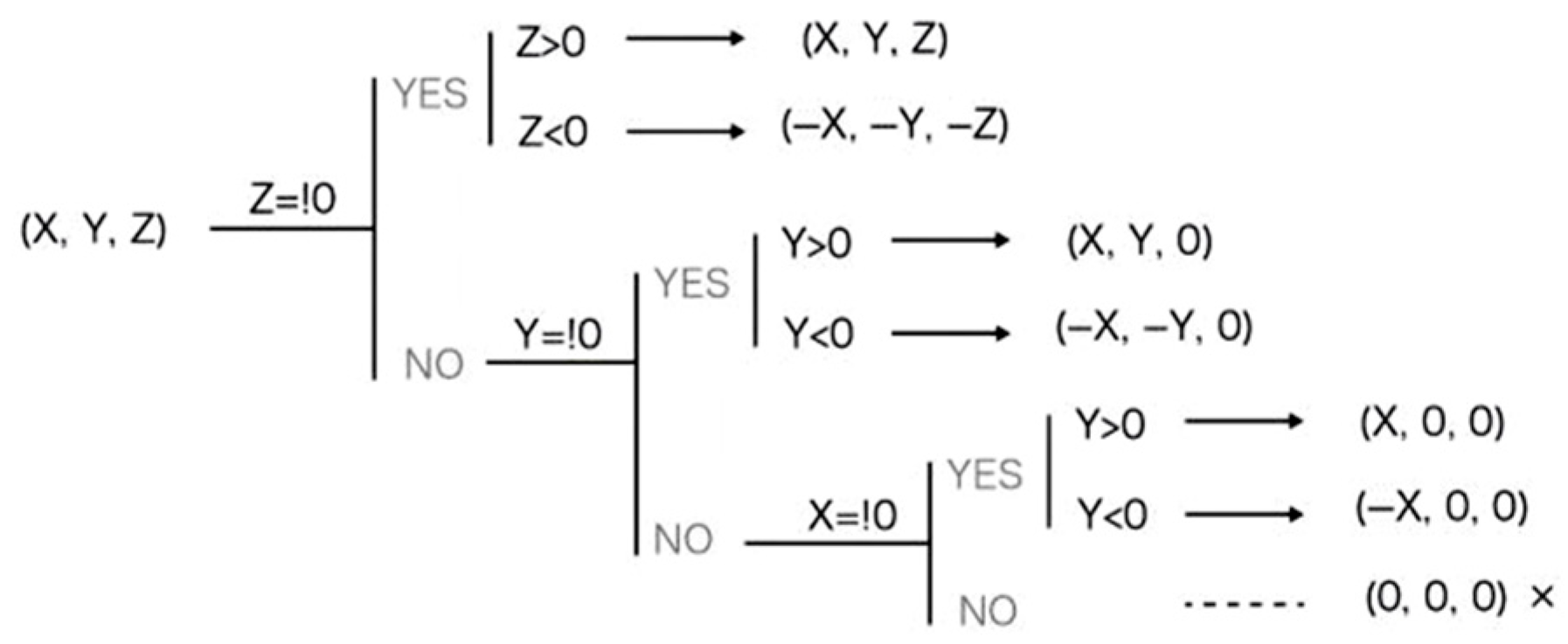
  • Unify the directional vectors: Determine whether the vector lies in the upper hemisphere. Retain vectors that meet this condition, reverse and store those that do not, and address any special cases related to other boundary conditions (Figure 2).
  • Transform the coordinate system: Transform the vectors from Cartesian coordinates to Spherical coordinates using the following formulas: set the radius r = 1, calculate the polar angle θ = arccos(Z), and compute the azimuthal angle ϕ = arctan(Y/X).

3.4. Calculation of Vector Distribution Probability

Then, the probabilities of the vectors distributed in each spatial unit need to be calculated, which involves the following:
  • Determine the spatial unit to which each directional vector belongs: Traverse the direction vectors of the streets, use the polar angleθand azimuthal angle ϕ to determine the corresponding spatial range, and increment the count accordingly. After completing the traversal, the count of vectors within each spatial range can be accurately obtained.
  • Count the total number of vectors.
  • Calculate the probability of vectors appearing in each spatial unit: Divide the number of vectors in each spatial range by the total number of vectors.
It is worth noting that, first, Pandas’ built-in statistical function “value counts” can be used for fast statistical analysis, providing better performance than manually implemented methods. Additionally, the processing speed can be improved by using Pandas’ “apply” method to batch process data, reducing the number of loops needed. Second, when determining the spatial range of a vector, utilizing NumPy’s efficient computational capabilities to define angle ranges and handle small values can greatly enhance code execution efficiency.

3.5. Calculation of Three-Dimensional Orientation Entropy

Finally, the entropy can be calculated. By substituting the probabilities P(X) of non-zero vector distributions into the formula for information entropy (Equation (1)) and accumulating, the entropy value of these vectors can be obtained. In the current scenario, where space is divided into 512 units, the maximum value of three-dimensional orientation entropy is 9, which occurs when the vectors are evenly distributed across all units [5].
The “scipy.stats.entropy” function with the “base = 2” parameter can be used to calculate the entropy value, eliminating the necessity of manually defining the formula.

4. Results and Discussion

4.1. Entropy Values for Representative Areas in Selected Chinese Cities

Ten major cities in China were selected, with each city’s representative being an administrative district known for its historical and cultural characteristics. Based on the calculation steps outlined above, three-dimensional orientation entropy values for these ten districts were calculated using OSM (OpenStreetMap) road network data and GDEMV3 30 M (Global Digital Elevation Model v3, 30 m resolution) [10,24].
Returning to the definition of the concept, information entropy measures the amount of information required to fully understand the system [5]. In other words, the higher the three-dimensional orientation entropy of a certain area, the more information is needed to understand the distribution of street directions in space, making it more difficult to fully comprehend the street network. This suggests that the higher the three-dimensional orientation entropy of a street network, the more chaotic the streets appear, implying a positive correlation between the objective value (entropy) and the subjective perception of disorder [3].
The entropy calculation results align with the above expectations (Table 1). For example, Beijing, characterized by flat terrain and a simple, clear grid road network, has the lowest entropy value in its Dongcheng District, at 5.78275223657532. In contrast, Chongqing, known for its hilly terrain and complex street layout, has the highest entropy value in its Yuzhong District, at 7.49360245117109. The other cities fall between these two extremes, such as Hangzhou’s Xihu District, which has a mid-range entropy value of 6.48025188538720 (Table 1, Figure 3).

4.2. Perceptual Impact of Entropy Values in High-Entropy Areas: A Case Study of Chongqing’s Central Urban Area

Referring to patterns observed in other research in environmental psychology, particularly the stimulus–response theory, it is believed that the impact of environmental stimuli on individuals follows an inverted U-shape. When the stimulus intensity is either too low or too high, the response is not significant, but at an optimal intensity, the response is most pronounced. In this study, the central urban area of Chongqing was selected to explore the correlation between three-dimensional orientation entropy and the public’s perception of street disorder. This further investigates the nature of the indicator under conditions of extremely high entropy values [3].

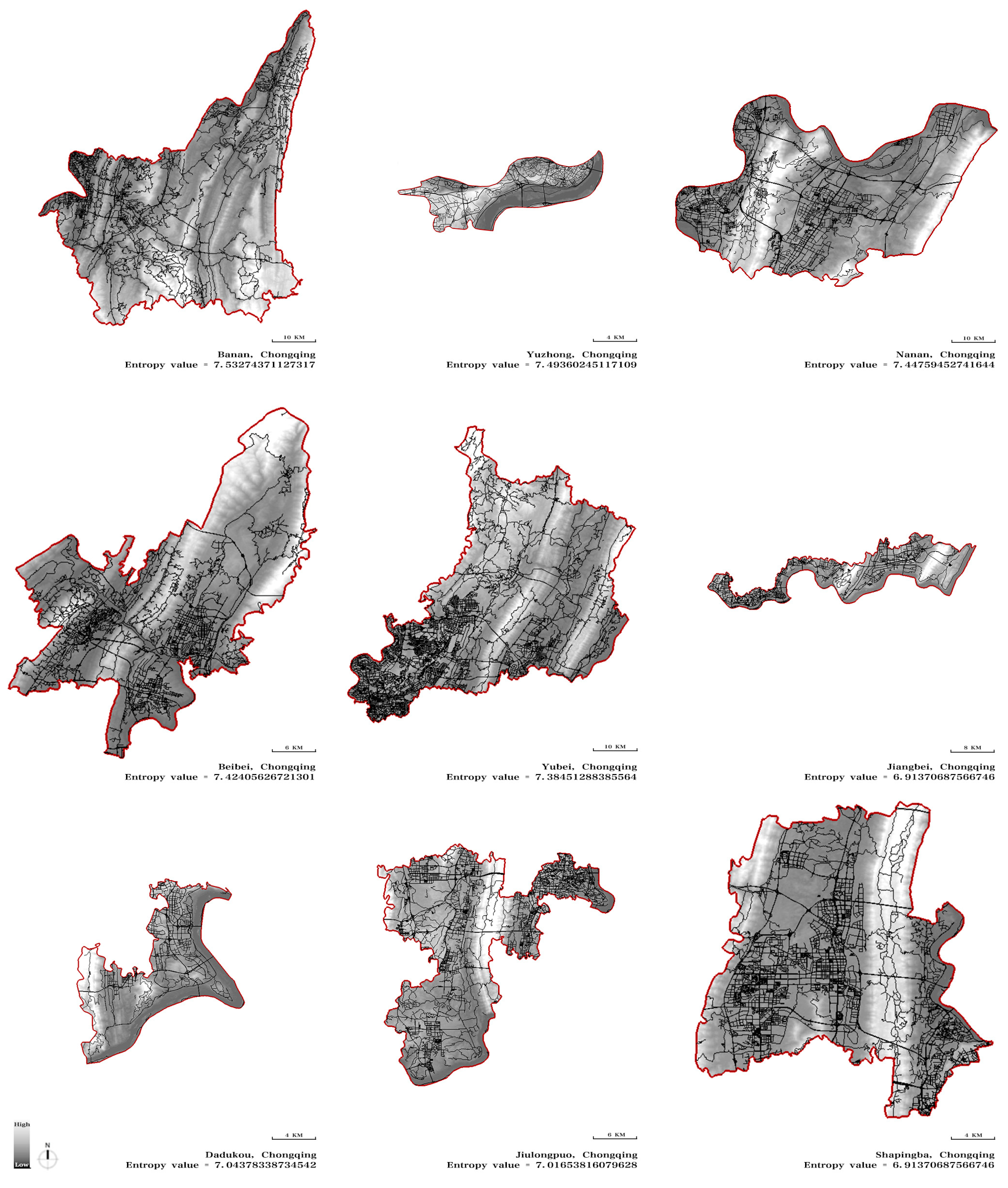
4.2.1. Three-Dimensional Orientation Entropy of Streets in the Districts of Downtown Chongqing

Three-dimensional orientation entropy values for nine districts of downtown Chongqing were calculated using OSM (OpenStreetMap) road network data and GDEMV3 30 M (Global Digital Elevation Model v3, 30 m resolution) (Table 2, Figure 4) [22,24].

4.2.2. Perception of Disorderliness of Streets in the Districts of Downtown Chongqing

A third-party survey organization, WJX, was commissioned to select individuals who have been driving for more than 2 years, have lived in the main urban area of Chongqing for the past 2 years, and frequently drive cars for commuting, as our respondents. We obtained their subjective assessment of the level of disorder in the streets of the nine central districts of Chongqing through the questionnaire. The scoring criteria were stipulated as follows: 1 point for “very clear,” 5 points for “average,” and 10 points for “very chaotic.” (Appendix A).
We collected 104 valid responses. The final score was determined by calculating the average score given by each respondent (Table 3).

4.2.3. Correlation Between Entropy and Subjective Ratings

Here, the Spearman’s rank correlation coefficient method was chosen to quantify the correlation between the “three-dimensional orientation entropy” and the “subjective ratings of street disorderliness.” (Table 4).
The Spearman’s rank correlation coefficient of −0.4167 suggests a moderate negative association between three-dimensional orientation entropy and perceived street disorderliness. However, the corresponding p-value of 0.2646 exceeds the commonly accepted threshold of statistical significance (p < 0.05), indicating that the observed relationship could plausibly occur by chance under the null hypothesis. As such, we cannot confidently assert the presence of a statistically significant correlation based on the current data.
Given the small sample size and the exploratory nature of this case study, these results should be interpreted with caution. Rather than offering definitive conclusions, the findings point to a potential trend that warrants further investigation and validation across larger, more diverse urban settings. This study is intended as a proof-of-concept to assess the applicability of a three-dimensional orientation entropy metric in perceptual analyses of street networks.
Taken together, the coefficient and p-value do not support a robust negative correlation in the context of extremely high entropy values. However, they do reveal that three-dimensional orientation entropy is not consistently or positively aligned with subjective evaluations—challenging the assumption that spatial complexity, as captured by entropy, necessarily translates to higher perceived disorder. This insight should inform the cautious use of entropy-based indicators in urban design assessment.
While orientation entropy, by its theoretical definition and the prior validation in Section 4.1, is expected to influence perception of street layout, subjective judgments of disorderliness are also shaped by a range of other factors, including visual clutter, maintenance, and contextual cues at the street level. Consequently, the relationship between entropy and perceived disorder is unlikely to be linear or one-dimensional. It demands a broader, integrative framework that considers multiple layers of perceptual and environmental variables [3].
Moreover, limitations in the experimental design may have attenuated observable correlations. Although the sample size of 104 respondents provides a reasonable basis for analysis, the participants were selected based on specific criteria, including having driven for more than two years, residing in Chongqing’s main urban area for the past two years, and frequently commuting by car. While these criteria ensured respondents’ familiarity with the study context, they may also introduce some demographic homogeneity, potentially limiting the generalizability of findings. Additionally, the perceptual task used static street-view images rather than immersive or dynamic environments, which may have constrained participants’ sensitivity to subtle spatial cues such as volumetric articulation or directional irregularity. Together, these factors may have reduced the measurable impact of orientation entropy on subjective evaluations [12].
In addition, the perceptual task used static street-view images rather than immersive or dynamic environments, which may have constrained participants’ sensitivity to subtle spatial cues such as volumetric articulation or directional irregularity. Together, these factors—sample homogeneity and limited perceptual engagement—likely reduced the measurable impact of orientation entropy on subjective evaluations.
For example, in our observations, hillside areas tended to exhibit higher three-dimensional orientation entropy, yet these areas also presented greater navigation challenges, suggesting a complex interplay between spatial complexity and navigability. Additionally, certain neighborhoods with high entropy values did not correspond to higher perceived disorder, indicating that the relationship between spatial complexity and subjective evaluations may be nonlinear or context-dependent [17].
The current study’s limited sample size and single-time-point data collection constrain the ability to detect statistically significant correlations. Conducting multi-temporal studies with larger and more diverse participant pools may reveal more robust and generalizable patterns, enabling a deeper understanding of the linkage between three-dimensional orientation entropy and perceptual outcomes.
Prior research has demonstrated that spatial complexity, particularly in hillside or irregular urban environments, complicates navigation and perception. Classic spatial syntax theory (Hillier & Hanson, 1984) [11] and network analysis further underscore the nuanced interplay between spatial structure and human experience. Moreover, Montello highlights the importance of longitudinal and diverse sampling in navigation research, supporting the call for multi-temporal, larger-scale studies [9,25].

4.3. Comparison with Traditional Spatial Complexity Measures

The proposed three-dimensional orientation entropy complements existing spatial complexity metrics from different analytical dimensions. Traditional space syntax indicators, such as integration and connectivity, emphasize accessibility and route choice preference within planar network structures. These measures have proven valuable for modeling pedestrian and vehicular flows but generally do not account for the vertical and directional complexity inherent in three-dimensional urban environments [6,11,26,27].
Fractal dimension, in contrast, measures morphological self-similarity, offering insights into the formal and visual complexity of spatial patterns. While useful for characterizing form-based complexity, it lacks sensitivity to directional heterogeneity in navigable space [13,26].
Three-dimensional orientation entropy bridges this gap by capturing the diversity and distribution of street segment orientations in three-dimensional space. It provides a unique angle of analysis focused on spatial directionality, especially valuable in topographically complex urban contexts such as Chongqing [7,15].
Each of these indicators reflects distinct aspects of spatial order—connectivity, morphology, and directionality. Their integration holds potential for constructing a more comprehensive framework for urban complexity assessment. Future studies may explore the synergies between these metrics, particularly in predicting environmental perception, navigation difficulty, and spatial legibility in urban design [6,13,28].

5. Conclusions

This study proposed a novel computational framework for quantifying three-dimensional orientation entropy in urban street networks. By integrating elevation data, the method captures spatial complexity more comprehensively, particularly in topographically diverse cities. A case study in Chongqing demonstrates the framework’s potential to reveal structural nuances related to urban spatial order and environmental perception.
This framework offers a replicable, theoretically grounded tool that can aid urban design and planning in complex terrain contexts.

6. Research Limitations and Future Directions

6.1. Limitations of ArcGIS and Python Toolchain

The 3D orientation entropy calculation workflow in this study relies on the ArcGIS 10.8 platform and Python 3.10.10 scripts, which introduces several constraints. ArcGIS is commercial software requiring licenses, limiting the accessibility and broad adoption of the research tools by urban planners and scholars. Additionally, Python scripts exhibit performance bottlenecks when processing large-scale 3D data, particularly in voxel grid partitioning and directional statistics, resulting in lengthy computation times and reduced batch processing efficiency.
Moreover, the current implementation depends heavily on the ArcGIS Pro environment, making it challenging to port the workflow to open-source GIS platforms or pure Python environments, thus limiting code portability and collaborative development. Furthermore, the existing codebase lacks a packaged, user-friendly interface, raising operational barriers for practitioners without programming expertise.

6.2. Detailed Research Limitations

While this study provides an in-depth analysis of three-dimensional orientation entropy in typical hillside neighborhoods of Chongqing, it is subject to some limitations. The research area is restricted to specific hillside blocks and does not cover plains, coastal cities, or densely built high-rise environments, which limits the generalizability of the results [6,29]. The method uses fixed voxel sizes and angular divisions, potentially overlooking multi-scale spatial structures and underestimating hierarchical spatial complexity [14,30].
In addition, the reliance on ArcGIS-specific 3D data formats imposes data conversion and precision constraints, limiting the completeness of urban spatial representation. The perception survey includes a relatively small and demographically narrow sample, potentially affecting the statistical power and universality of conclusions. Moreover, the study analyzes static spatial structures and does not consider temporal dynamics or dynamic spatial behaviors that may influence orientation entropy and perception.

6.3. Recommendations for Future Research

To address current limitations, future research should extend the validation of the 3D orientation entropy metric to multiple cities with diverse terrains, thereby testing its universality and robustness. Employing multi-scale spatial partitioning will allow for a more nuanced capture of hierarchical spatial structures. Integration of high-precision data sources, such as LiDAR and detailed 3D urban models, is recommended to improve spatial representation accuracy [10,30].
Since the present study focuses on hillside urban environments, its applicability to other urban typologies—such as flat plains, dense high-rise districts, and waterfront cities—remains to be verified. Future efforts will include applying and adapting the methodology to cities like Hong Kong and San Francisco to evaluate and enhance its generalizability.
Moreover, expanding perception data collection to incorporate dynamic tracking and behavioral analysis will provide deeper insights into temporal and experiential dimensions of spatial orientation, thereby strengthening the metric’s relevance for urban design and planning applications [12]. In this regard, advanced visual similarity metrics, such as fast Earth mover’s distance (EMD) techniques developed for catadioptric image sequences, may offer new tools for analyzing spatial perception dynamics in complex urban environments [23].

Author Contributions

Conceptualization, H.R., L.C. and C.L.; Methodology, H.R.; Software, H.R.; Validation, H.R.; Formal analysis, H.R. and L.C.; Investigation, H.R.; Resources, L.C.; Data curation, H.R.; Writing—original draft, H.R.; Writing—review & editing, C.L.; Visualization, L.C.; Supervision, C.L.; Project administration, H.R. and C.L.; Funding acquisition, C.L. All authors have read and agreed to the published version of the manuscript.

Funding

This research is supported by the Project of Philosophy and Social Science Planning of Zhejiang Province (23NDJC076YB), Research Program of Humanities and Social Sciences of the Ministry of Education (24YJA840008), and ZJU-STEC Urban Development and Planning Innovation Joint Research Center Project (Grant No.513000-I5220A/001).

Institutional Review Board Statement

Ethical review and approval were waived for this study due to the nature of the anonymous, non-invasive perception experiments, which did not involve any personally identifiable information or sensitive human data. According to the ethics review guidelines for social science research at Zhejiang University, such studies do not require formal ethical approval.

Informed Consent Statement

Informed consent was obtained from all subjects involved in the study.

Data Availability Statement

The data and Python scripts supporting this study are available at Zenodo (https://doi.org/10.5281/zenodo.15294711). Additional publicly available datasets were used: OpenStreetMap (https://www.openstreetmap.org) under the Open Database License (ODbL). GDEMV3 30M from the Geospatial Data Cloud (http://www.gscloud.cn).

Conflicts of Interest

All authors declare that the research was conducted in the absence of any commercial or financial relationships that could be construed as a potential conflict of interest.

Appendix A. English Translation of the Questionnaire

Title:
Please Rate the Level of Disorderliness of the Road Network in Downtown Chongqing
Survey Information:
We sincerely invite you to participate in this survey and hope that you can fill it out patiently. The results will be used in an urban design research project being conducted by the College of Civil Engineering and Architecture, Zhejiang University. This survey is anonymous, and we kindly ask you to rate the level of disorderliness of the road network in downtown Chongqing. There are no right or wrong answers; please fill in the score based on your true feelings. The survey consists of up to 11 multiple-choice questions and is expected to take about 3 min to complete.
Instructions:
The score should be an integer between 1 and 10, specifically including 1, 2, 3, 4, 5, 6, 7, 8, 9, 10. A higher score indicates a higher level of disorderliness in the streets of the area. A score of 1 means the roads are very clear, 5 means the roads are average, and 10 means the roads are very chaotic.
Buildings 15 02460 i001
1.
Do you agree to participate in this survey based on the information provided above? [Single Choice]*
Agree (Please continue answering)
Disagree (The survey will be closed, thank you for your participation)
P.S. If the participant selects the first option of Question 1, the survey will continue. If the participant selects the second option of Question 1, the survey will stop and exit.
———————————————————————————————————————
2.
In the following districts of downtown Chongqing, please select the ones you are particularly unfamiliar with (you may choose none if you are familiar with all of them) [Multiple Choice]*
Yuzhong District
Dadukou District
Jiangbei District
Shapingba District
Jiulongpuo District
Nanan District
Beibei District
Yubei District
Banan District
None
———————————————————————————————————————
3.
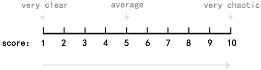
Rate the level of disorderliness of the road network in Yuzhong District [Single Choice]*
1 (Very clear)
2
3
4
5 (Average)
6
7
8
9
10 (Very chaotic)
P.S. If the participant selects the first option of Question 2, this question will not be displayed.
4.
Rate the level of disorderliness of the road network in Dadukou District [Single Choice]*
1 (Very clear)
2
3
4
5 (Average)
6
7
8
9
10 (Very chaotic)
P.S. If the participant selects the second option of Question 2, this question will not be displayed.
5.
Rate the level of disorderliness of the road network in Jiangbei District [Single Choice]*
1 (Very clear)
2
3
4
5 (Average)
6
7
8
9
10 (Very chaotic)
P.S. If the participant selects the third option of Question 2, this question will not be displayed.
6.
Rate the level of disorderliness of the road network in Shapingba District [Single Choice]*
1 (Very clear)
2
3
4
5 (Average)
6
7
8
9
10 (Very chaotic)
P.S. If the participant selects the fourth option of Question 2, this question will not be displayed.
7.
Rate the level of disorderliness of the road network in Jiulongpuo District [Single Choice]*
1 (Very clear)
2
3
4
5 (Average)
6
7
8
9
10 (Very chaotic)
P.S. If the participant selects the fifth option of Question 2, this question will not be displayed.
8.
Rate the level of disorderliness of the road network in Nanan District [Single Choice]*
1 (Very clear)
2
3
4
5 (Average)
6
7
8
9
10 (Very chaotic)
P.S. If the participant selects the sixth option of Question 2, this question will not be displayed.
9.
Rate the level of disorderliness of the road network in Beibei District [Single Choice]*
1 (Very clear)
2
3
4
5 (Average)
6
7
8
9
10 (Very chaotic)
P.S. If the participant selects the seventh option of Question 2, this question will not be displayed.
10.
Rate the level of disorderliness of the road network in Yubei District [Single Choice]*
1 (Very clear)
2
3
4
5 (Average)
6
7
8
9
10 (Very chaotic)
P.S. If the participant selects the eighth option of Question 2, this question will not be displayed.
11.
Rate the level of disorderliness of the road network in Banan District [Single Choice]*
1 (Very clear)
2
3
4
5 (Average)
6
7
8
9
10 (Very chaotic)
P.S. If the participant selects the ninth option of Question 2, this question will not be displayed.
Thank you again for your patience in completing the survey. You have finished all the questions. Please click the button below to submit.
P.S. After the participant completes all the required questions and clicks the submit button, the questionnaire responses will be uploaded and recorded.

References

  1. Gudmundsson, A.; Mohajeri, N. Entropy and order in urban street networks. Sci. Rep. 2013, 3, 3324. [Google Scholar] [CrossRef] [PubMed]
  2. Batty, M. Entropy in Spatial Aggregation. Geogr. Anal. 1976, 8, 1–21. [Google Scholar] [CrossRef]
  3. Haken, H.; Portugali, J. The Face of the City Is Its Information. J. Environ. Psychol. 2003, 23, 385–408. [Google Scholar] [CrossRef]
  4. Gastner, M.T.; Newman, M.E. The spatial structure of networks. Eur. Phys. J. B 2006, 49, 247–252. [Google Scholar] [CrossRef]
  5. Shannon, C.E. A mathematical theory of communication. SIGMOBILE Mob. Comput. Commun. Rev. 2001, 5, 3–55. [Google Scholar] [CrossRef]
  6. Boeing, G. Urban spatial order: Street network orientation, configuration, and entropy. Appl. Netw. Sci. 2019, 4, 67. [Google Scholar] [CrossRef]
  7. Xie, F.; Levinson, D. Measuring the Structure of Road Networks. Geogr. Anal. 2007, 39, 336–356. [Google Scholar] [CrossRef]
  8. Chan, S.H.Y.; Donner, R.V.; Lämmer, S. Urban road networks—Spatial networks with universal geometric features? Eur. Phys. J. B 2011, 84, 563–577. [Google Scholar] [CrossRef]
  9. Turner, A.; Doxa, M.; O’SUllivan, D.; Penn, A. From Isovists to Visibility Graphs: A Methodology for the Analysis of Architectural Space. Environ. Plan. B Plan. Des. 2001, 28, 103–121. [Google Scholar] [CrossRef]
  10. Aleksandrov, M.; Zlatanova, S.; Kimmel, L.; Barton, J.; Gorte, B. Voxel-Based Visibility Analysis for Safety Assessment of Urban Environments. ISPRS Ann. Photogramm. Remote. Sens. Spat. Inf. Sci. 2019, IV-4/W8, 11–17. [Google Scholar] [CrossRef]
  11. Hillier, B.; Hanson, J. The Social Logic of Space; Cambridge University Press: Cambridge, UK, 1984. [Google Scholar]
  12. Stamps, A.E. Use of Static and Dynamic Media to Simulate Environments: A Meta-Analysis. Percept. Mot. Ski. 2010, 111, 355–364. [Google Scholar] [CrossRef] [PubMed]
  13. Boeing, G. The Morphology and Circuity of Walkable and Drivable Street Networks. In The Mathematics of Urban Morphology; D’Acci, L., Ed.; Modeling and Simulation in Science, Engineering and Technology; Birkhäuser: Cham, Switzerland, 2019; pp. 271–287. [Google Scholar]
  14. Boeing, G. Measuring the complexity of urban form and design. Urban Des. Int. 2018, 23, 281–292. [Google Scholar] [CrossRef]
  15. Hanson, J. Order and Structure in Urban Design. Ekistics 1989, 56, 22–42. [Google Scholar]
  16. Manioudis, M.; Meramveliotakis, G. Broad strokes towards a grand theory in the analysis of sustainable development: A return to the classical political economy. New Polit. Econ. 2022, 27, 866–878. [Google Scholar] [CrossRef]
  17. Klarin, T. The Concept of Sustainable Development: From its Beginning to the Contemporary Issues. Zagreb Int. Rev. Econ. Bus. 2018, 21, 67–94. [Google Scholar] [CrossRef]
  18. Courtat, T.; Gloaguen, C.; Douady, S. Mathematics and Morphogenesis of Cities: A Geometrical Approach. Phys. Rev. E 2011, 83, 036106. [Google Scholar] [CrossRef]
  19. Duan, Y.; Lu, F. Robustness of City Road Networks at Different Granularities. Phys. A Stat. Mech. Its Appl. 2014, 411, 21–34. [Google Scholar] [CrossRef]
  20. Boeing, G. Planarity and street network representation in urban form analysis. Environ. Plan. B Urban Anal. City Sci. 2018, 47, 855–869. [Google Scholar] [CrossRef]
  21. Neumann, J. The Topological Information Content of a Map: An Attempt At A Rehabilitation Of Information Theory In Cartography. Cartographica 1994, 31, 26–34. [Google Scholar] [CrossRef]
  22. Li, W.; Hu, D.; Liu, Y. An Improved Measuring Method for the Information Entropy of Network Topology. Trans. GIS 2018, 22, 1632–1648. [Google Scholar] [CrossRef]
  23. Tahri, O.; Usman, M.; Demonceaux, C.; Fofi, D.; Hittawe, M. Fast Earth Mover’s Distance Computation for Catadioptric Image Sequences. In Proceedings of the 2016 IEEE International Conference on Image Processing (ICIP), Phoenix, AZ, USA; 2016; pp. 2485–2489. [Google Scholar] [CrossRef]
  24. Boeing, G. OSMnx: New Methods for Acquiring, Constructing, Analyzing, and Visualizing Complex Street Networks. Comput. Environ. Urban Syst. 2017, 65, 126–139. [Google Scholar] [CrossRef]
  25. Barron, C.; Neis, P.; Zipf, A. A Comprehensive Framework for Intrinsic OpenStreetMap Quality Analysis. Trans. GIS 2013, 18, 877–895. [Google Scholar] [CrossRef]
  26. Hillier, B. Space Is the Machine: A Configurational Theory of Architecture; Cambridge University Press: Cambridge, UK, 1996. [Google Scholar]
  27. Hillier, B. Space Syntax: A Different Urban Perspective. Archit. Res. Q. 2007, 11, 287–291. [Google Scholar]
  28. Barthélemy, M. Spatial Networks. Phys. Rep. 2011, 499, 1–101. [Google Scholar] [CrossRef]
  29. Boeing, G. A multi-scale analysis of 27,000 urban street networks: Every US city, town, urbanized area, and Zillow neighborhood. Environ. Plan. B Urban Anal. City Sci. 2018, 47, 590–608. [Google Scholar] [CrossRef]
  30. Tsiotas, D.; Polyzos, S. The Complexity in the Study of Spatial Networks: An Epistemological Approach. Netw. Spat. Econ. 2017, 18, 1–32. [Google Scholar] [CrossRef]
Figure 1. Schematic diagram of the hemispherical space and one of the spatial units.
Buildings 15 02460 g001
Figure 2. Schematic diagram of unification process.
Buildings 15 02460 g002
Figure 3. Overlay of DEM elevation and street network maps for Dongcheng District, Beijing (top), Xihu District, Hangzhou (middle), and Yuzhong District, Chongqing (bottom).
Buildings 15 02460 g003
Figure 4. Overlay of DEM elevation and street network maps for the districts of downtown Chongqing.
Buildings 15 02460 g004
Table 1. Three-dimensional orientation entropy values of representative districts in ten major Chinese cities.
CityDistrictEntropy Value
BeijingDongcheng5.78275223657532
ShanghaiHuangpu5.88844425575119
TianjinHeping6.41459920001745
NanjingGulou6.45663309843272
HangzhouXihu6.48025188538720
ShenzhenNanshan6.50404792121149
WuhanJianghan6.74568743177610
ChengduJinjiang6.95121621799309
GuangdongGuangzhou7.14797931697683
ChongqingYuzhong7.49360245117109
Table 2. The three-dimensional street orientation entropy values of downtown Chongqing.
DistrictEntropy Value
Banan7.53274371127317
Yuzhong7.49360245117109
Nanan7.44759452741644
Beibei7.42405626721301
Yubei7.38451288385564
Jiangbei7.38030436371737
Dadukou7.04378338734542
Jiulongpuo7.01653816079628
Shapingba6.91370687566746
Table 3. The subjective assessment values of street disorderliness in downtown Chongqing.
DistrictSubjective ValueNumber of Raters
Shapingba5.82100
Yuzhong5.7798
Jiulongpuo5.2495
Nanan5.0583
Yubei4.9190
Jiangbei4.7992
Dadukou4.7492
Beibei4.684
Banan4.5685
Table 4. Results of the Spearman’s rank correlation coefficient method.
Spearman’s Rank Correlation Coefficient−0.4167
p-value0.2646
Disclaimer/Publisher’s Note: The statements, opinions and data contained in all publications are solely those of the individual author(s) and contributor(s) and not of MDPI and/or the editor(s). MDPI and/or the editor(s) disclaim responsibility for any injury to people or property resulting from any ideas, methods, instructions or products referred to in the content.

