Uncertainty Analysis and Risk Assessment for Variable Settlement Properties of Building Foundation Soils

Abstract

Settlement analyses of foundation soils are very important for the investigation, design, and construction of buildings. However, due to complex natural sedimentary processes, soil-forming environments, and geological tectonic stress histories, settlement properties show obvious spatial variability and autocorrelation. Moreover, measurement data on the physical and mechanical parameters of building foundation soils are limited. This limits the accuracy of formation stability analyses and safety evaluations. In this study, a series of field tests of building foundation soils were carried out, and the statistical physical and mechanical properties of the clay strata were obtained. A random field method and copula functions of uncertain geotechnical properties with limited survey data are proposed. A dual-yield surface constitutive model of the soil properties and a stability analysis method for uncertain deformation were developed. The detailed analytical procedures for soil deformation and stratum settlement are presented. The reliability functions and failure probabilities of variable settlement processes are calculated and analyzed. The impact of the spatial variation and cross-correlation of geotechnical properties on the probabilistic stability of variable land subsidence is discussed. This work presents an innovative analysis approach for evaluating the variable settlement properties of building foundation soils. The results show that the four different mechanical parameters can be regressed to linear equations. The horizontal fluctuation scale is significantly larger than the vertical scale. Copula theory provides a powerful framework for modeling limited geotechnical parameters. The bootstrap approach avoids parametric assumptions, leveraging empirical data to enhance the reliability analysis of variable settlement. The variability parameter exerts a greater influence on land subsidence processes than the correlation structure. The failure probabilities of variable stratum settlement for different cross-correlations of building foundation soils are different. These results provide an important reference for the safety of building engineering.

1. Introduction

Building foundation soil settlement deformation primarily stems from the interaction between the applied structural loads and soil properties. When heavy loads compress loose, water-saturated soil (e.g., clay), the pore water initially resists the volume change, creating excess pore pressure. As this pressure dissipates over time, soil particles rearrange, causing consolidation—a gradual reduction in the void space that manifests as downward settlement. The rate and magnitude depend on the soil permeability, load intensity, and drainage conditions, with slow-draining clays often experiencing prolonged, differential settlement [1,2,3]. A critical characteristic lies in its spatial heterogeneity, manifested through uneven settlement patterns caused by variations in the subsurface stratigraphy. Compressible clay layers, for example, may produce localized subsidence bowls, while more competent sandy strata show resistant behavior. The phenomenon demonstrates material-dependent responses, with organic-rich soils exhibiting creep deformation and granular materials showing more immediate compression. The irreversible nature of most subsidence processes, particularly those involving clay-layer compaction, poses significant challenges for remediation. Furthermore, the threshold behavior observed in many subsidence systems means that ground deformation may accelerate dramatically after certain stress thresholds are exceeded [4,5,6]. Deng et al. [7] reveals the interactive effects between subsidence and other engineering geological disasters. The scale-dependent manifestation of subsidence, from millimeter-scale annual settlements in regional basins to meter-level sudden collapses in mining areas, necessitates tailored assessment approaches [7]. These characteristics collectively contribute to the nonlinear settlement properties of building foundation soils, requiring sophisticated numerical modeling that incorporates stochastic material properties and complicated mechanical processes for accurate prediction and mitigation [8,9]. The prerequisite for the settlement analysis of foundation soil is the accurate characterization of the geotechnical properties.

However, Zevgolis et al. and Nguyen et al. found that building foundation soils exhibit inherent spatial variability and complex correlation structures due to their natural depositional processes, geological histories, and environmental conditions [10,11]. Spatial variability refers to the heterogeneous distribution of key properties (e.g., compressibility, permeability, and shear strength) across different locations, even within seemingly uniform strata [12]. This variability is often characterized by random field models, where autocorrelation functions quantify how the material properties vary with distance and direction. For instance, clay layers may show strong vertical correlations due to sedimentation patterns but weaker horizontal correlations [13]. Moreover, interdependencies between parameters such as the porosity and hydraulic conductivity give rise to cross-correlations, further complicating the mechanical and hydraulic behavior of subsurface materials. These spatial characteristics exert a significant influence on land subsidence patterns. In regions with highly compressible yet poorly correlated soils (e.g., discontinuous soft clay lenses), uneven settlement may occur, leading to differential subsidence and ground fissures. Conversely, in aquifer systems, the spatial correlation of the permeability governs the groundwater flow and pressure distribution, affecting the rate and extent of the consolidation-induced subsidence [14,15,16]. Guan et al. and Li et al. found that the key points for analyzing variable land subsidence processes are the characterization methods for the spatial variability and the correlation of geotechnical materials [17,18].

The random field theory provides a powerful mathematical framework to quantify the spatial variabilities and correlation structures of geotechnical materials, which are inherently heterogeneous due to natural deposition and environmental processes. Gaussian random fields are commonly employed, where the material properties (e.g., shear strength) are treated as spatially correlated random variables, characterized by a mean trend, variance, and an autocorrelation function [19,20,21]. The autocorrelation function defines how property correlations decay with separation distance, while the correlation length measures the spatial scale over which properties remain significantly dependent. Karhunen-Loève decomposition and Cholesky decomposition are used for the efficient discretization and simulation of random fields in finite element analyses. The cross-correlation between different parameters (e.g., the elastic modulus and Poisson’s ratio) is modeled using covariance matrices or copula theory. Conditional random fields integrate site investigation data through kriging or Bayesian updating to reduce uncertainty [22,23]. However, sample data information and different methods for characterizing variability and correlation have significant influences on uncertain geotechnical properties. The spatial variability and correlation of geotechnical materials are inherently linked to field and laboratory test data, which provide the basis for characterizing subsurface heterogeneity. Test data reveal localized property variations, while statistical methods extrapolate these measurements to quantify spatial trends and correlations. The autocorrelation structure defines how properties vary with distance, and the cross-correlation identifies interdependencies between parameters. However, sparse or unevenly distributed test data can lead to uncertainty in correlation models, necessitating Bayesian updating or machine learning to refine predictions [24,25,26]. Hence, the data structure and statistical correlation of the measured data need to be clarified, and the variable settlement properties of building foundation soils need to be discussed.

This research conducted multiple field tests on building foundation soils and derived the statistical physical and mechanical properties of the clay strata. To address the limited survey data, a random field method and copula functions were developed to characterize the uncertain geotechnical properties. Additionally, a dual-yield surface constitutive model for soil properties and a stability analysis method for uncertain deformations were formulated. The detailed analytical workflows for soil deformation and stratum settlement are also outlined. Furthermore, the reliability functions and failure probabilities of variable settlement processes were computed and examined. The influence of the spatial variability and cross-correlation among the geotechnical properties on the probabilistic stability of variable land subsidence was also explored. Collectively, this work introduces an innovative analytical approach for assessing the variable settlement characteristics of building foundation soils. The findings from this study offer valuable references for ensuring the safety of building engineering projects.

2. Field Experiment and Data Characteristics

Field testing and data interpretation are essential for characterizing spatially heterogeneous building foundation soils, as their properties vary significantly with location and depth. Traditional laboratory tests on limited samples often fail to capture this variability, leading to unreliable designs. Field tests, such as the CPT (Cone Penetration Test), the SPT (Standard Penetration Test), and geophysical surveys, provide continuous in situ data, revealing spatial trends and anomalies. Advanced data interpretation techniques, including statistical analysis and geostatistical modeling, help quantify the uncertainty and predict the soil behavior across the site. This approach ensures safer, cost-effective foundations by addressing the inherent soil variability, minimizing the risks of differential settlement or failure. Thus, integrating field testing with robust data interpretation is critical for accurate settlement assessments in heterogeneous conditions.

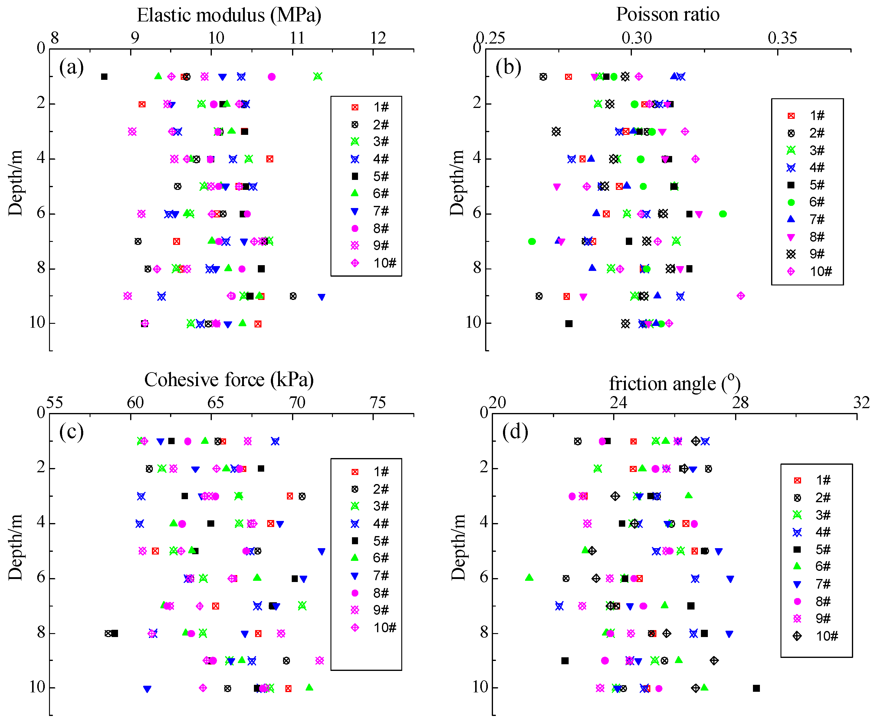
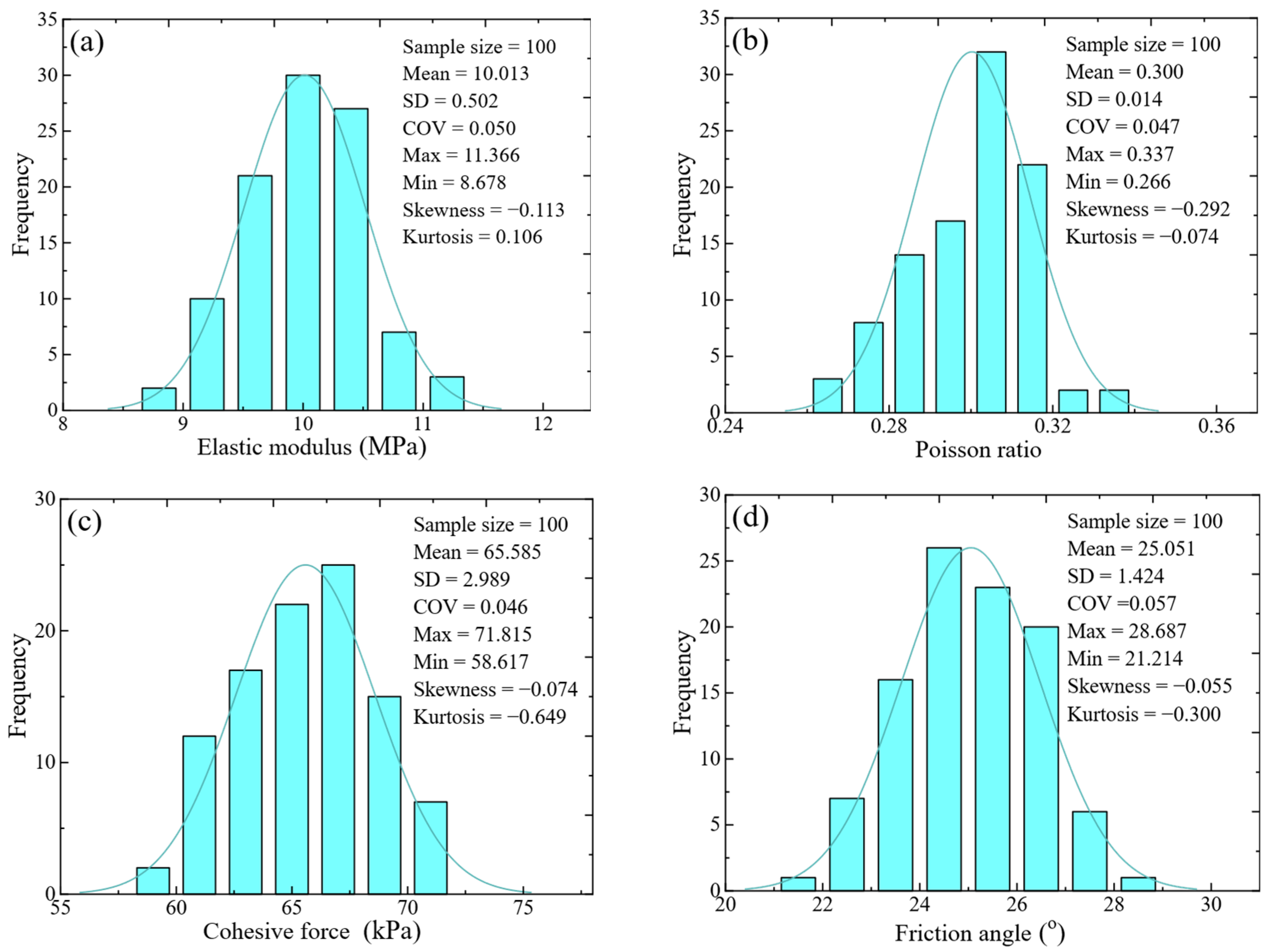
2.1. Test Procedure and Statistical Characteristics

The investigation areas are located in the northeastern part of Xuzhou City, Jiangsu Province, China, approximately 20 km from the city center. Geographically, they lie at the intersection of the Huanghuai Plain and the North China Plain, with coordinates around 34°18′ N latitude and 117°25′ E longitude. The investigation areas were historically a coal mining subsidence zone but have been transformed into an ecologically restored wetland, serving as a key environmental and recreational area. The site is underlain by Quaternary alluvial deposits, primarily consisting of silty clay, sandy silt, and fine sand layers. Due to past coal mining activities, some areas exhibit ground subsidence, leading to uneven settlement risks. Many buildings have been constructed. The area experiences a warm temperate monsoon climate, characterized by hot, humid summers (average: 27 °C) and cold, dry winters (average: 1 °C). The annual precipitation averages 800–900 mm, with most rainfall occurring from June to August. The soil-bearing capacity is generally moderate, requiring settlement assessments for new building engineering. The particle size distribution (PSD) and basic physical properties are fundamental indicators that govern the soil behavior and directly influence geotechnical engineering decisions. The PSD, which quantifies the relative proportions of gravel, sand, silt, and clay, determines critical characteristics such as the permeability, shear strength, compressibility, and frost susceptibility. Well-graded soils generally exhibit better engineering properties than those of poorly graded ones. The basic physical properties, including the water content, void ratio, specific gravity, and Atterberg limits (liquid limit, plastic limit, and plasticity index), provide essential insights into the soil consistency, density, and volume change potential. Sieve analysis involves shaking soil through a series of progressively smaller sieves, while hydrometer testing measures particle settling rates in suspension. This study conducted sampling within a depth range of 10 m of the stratum. Numbers were assigned at each 1 m depth. From 1 m to 10 m, they were sequentially labeled as 1# to 10#. Three different sample points were located in the investigation areas. To be specific, the coordinates of investigation area #1 are 34°22′04″ N latitude and 117°22′36″ E longitude. The coordinates of investigation area #2 are 34°22′12″ N latitude and 117°23′06″ E longitude. The coordinates of investigation area #3 are 34°21′52″ N latitude and 117°22′12″ E longitude.

Table 1. PSDs of soil in the investigation areas.

№	Particle Sizes and Their Percentages (%)
	<0.002 mm	0.002 mm~0.005 mm	0.005 mm~0.05 mm	0.05 mm~0.075 mm	>0.075 mm
1#	7.26	39.80	32.05	13.24	4.40
2#	8.16	41.96	32.13	14.64	3.83
3#	7.16	39.79	31.90	13.32	4.71
4#	7.39	39.99	32.17	15.69	3.91
5#	8.41	40.06	33.05	13.66	4.18
6#	9.38	41.28	32.13	12.55	4.50
7#	8.15	40.04	31.79	11.85	4.98
8#	9.23	39.89	32.31	13.89	4.79
9#	8.23	42.33	33.09	14.20	3.93
10#	8.27	40.17	31.62	13.01	4.34

presents the particle distributions of the soil in the investigation areas, obtained via the sieving method. Each value represents the average PSD of three different sample points. The PSD (0.002 mm~0.005 mm) is approximately 40%, and the PSD (0.05 mm~0.075 mm) is approximately 32%. The soil mass is basically in the state of cohesive soil.

The fundamental physical properties of soils, including the water content, specific gravity, density, and Atterberg limits (plastic limit, liquid limit), are measured through conventional geotechnical testing methods. To be specific, water content is determined by oven-drying, while specific gravity is tested using a pycnometer. Density is measured via a core cutter or sand replacement methods. Atterberg limits are obtained using the fall cone test for liquid and plastic limits.

Table 2. Physical properties of building foundation soils in the investigation areas.

№	Density (g/cm3)	Dry Density (g/cm3)	Moisture Content (%)	Specific Gravity of Solids	Plastic Limits (%)	Liquid Limits (%)
1#	1.77	1.37	29.16	2.67	20.48	41.07
2#	1.83	1.43	27.80	2.74	19.53	41.89
3#	1.91	1.47	29.81	2.78	19.24	38.67
4#	1.78	1.42	25.67	2.65	20.40	39.97
5#	1.99	1.51	31.84	2.58	19.16	38.67
6#	1.91	1.52	26.03	2.70	19.22	40.90
7#	1.94	1.52	28.02	2.75	19.64	40.60
8#	1.89	1.46	29.56	2.71	19.11	39.38
9#	1.54	1.18	30.74	2.83	20.34	39.33
10#	1.93	1.49	29.77	2.67	19.83	39.10

presents the test results of the physical properties of the soils in the investigation areas. The test results of the soils’ basic physical properties (water content, density, Atterberg limits, etc.) typically exhibit inherent variability due to the material heterogeneity, sampling disturbance, and testing conditions. Cohesive soils show greater dispersion in the plasticity indices, while granular soils demonstrate more consistent density measurements. This statistical dispersion follows normal or log-normal distributions, requiring probabilistic analysis for reliable geotechnical interpretations.

In situ soil testing plays a pivotal role in geotechnical engineering by providing accurate and representative data on soil properties under natural conditions, eliminating the disturbances caused by sampling and laboratory handling. Field test methods effectively capture the inherent spatial variability and anisotropy of soil layers, which are often overlooked in conventional lab tests [27,28]. For the cohesive soils of this study, the key mechanical parameters were determined through specialized in situ tests. The PMT provides direct measurements of the elastic modulus (EM) and Poisson’s ratio (PR) via an analysis of the pressure–deformation curve during cylindrical cavity expansion. The VST remains the gold standard for determining the cohesive force (CF) in soft clays through the controlled rotation of embedded blades. While the internal friction angle (FA) is challenging to measure directly in situ, the flat dilatometer test can estimate it through the correlation with the horizontal stress index. Figure 1 presents the measured geotechnical properties of the soil layers at different locations in the investigation areas. The discrete distribution of cohesive soils’ mechanical parameters primarily results from inherent material variability and testing complexities. Firstly, natural sedimentation creates heterogeneous microstructures with varying clay mineral compositions, organic contents, and void ratios, leading to spatial property fluctuations. Secondly, moisture sensitivity causes significant parameter changes with seasonal water content variations, as clay particle interactions are strongly water-dependent. Thirdly, thixotropic behavior means that the strength/stiffness properties depend on the loading history and rate, producing different values under various test conditions. Additionally, sampling disturbances disproportionately affect cohesive soils, altering their natural fabric and stress state. Understanding these statistical distributions is crucial for reliable safety assessments in foundation stability analyses.

The statistical distributions of cohesive soils’ mechanical parameters stem from multiple natural and experimental factors. Geologically, heterogeneous deposition environments create variations in mineral compositions, organic matter, and microstructures. Physically, moisture fluctuations alter interparticle forces and effective stresses, particularly in expansive clays. Mechanically, thixotropic effects cause time-dependent strength recovery post-disturbance. Experimentally, sampling methods inevitably disrupt natural fabric, while testing conditions influence measured values [29,30]. These factors collectively generate parameter distributions with characteristic variability. Such statistical behavior necessitates probabilistic design approaches for reliable geotechnical analysis. Figure 2 presents the statistical distribution of the measured geotechnical properties of the soil layer in the investigation area. For the EM, the maximum, minimum, and average are 11.366 MPa, 8.678 MPa, and 10.013 MPa, respectively. The standard deviation (SD), Skewness, and Kurtosis are 0.502 MPa, −0.113, and 0.106, respectively. For the PR, the maximum, minimum, and average are 0.337, 0.266, and 0.300, respectively. The SD, Skewness, and Kurtosis are 0.014, −0.292, and −0.074, respectively. For the CF, the maximum, minimum, and average are 71.815 kPa, 58.617 kPa, and 65.585 kPa, respectively. The SD, Skewness, and Kurtosis are 2.989 kPa, −0.074, and −0.649, respectively. For the FA, the maximum, minimum, and average are 28.687°, 21.214°, and 25.051°, respectively. The SD, Skewness, and Kurtosis are 1.424°, −0.055, and −0.300, respectively. The coefficients of variation of the four mechanical parameters are relatively close at approximately 0.05. It can be seen that the test data basically follow a normal distribution. However, it shows obvious variability and correlation, which require further characterization.

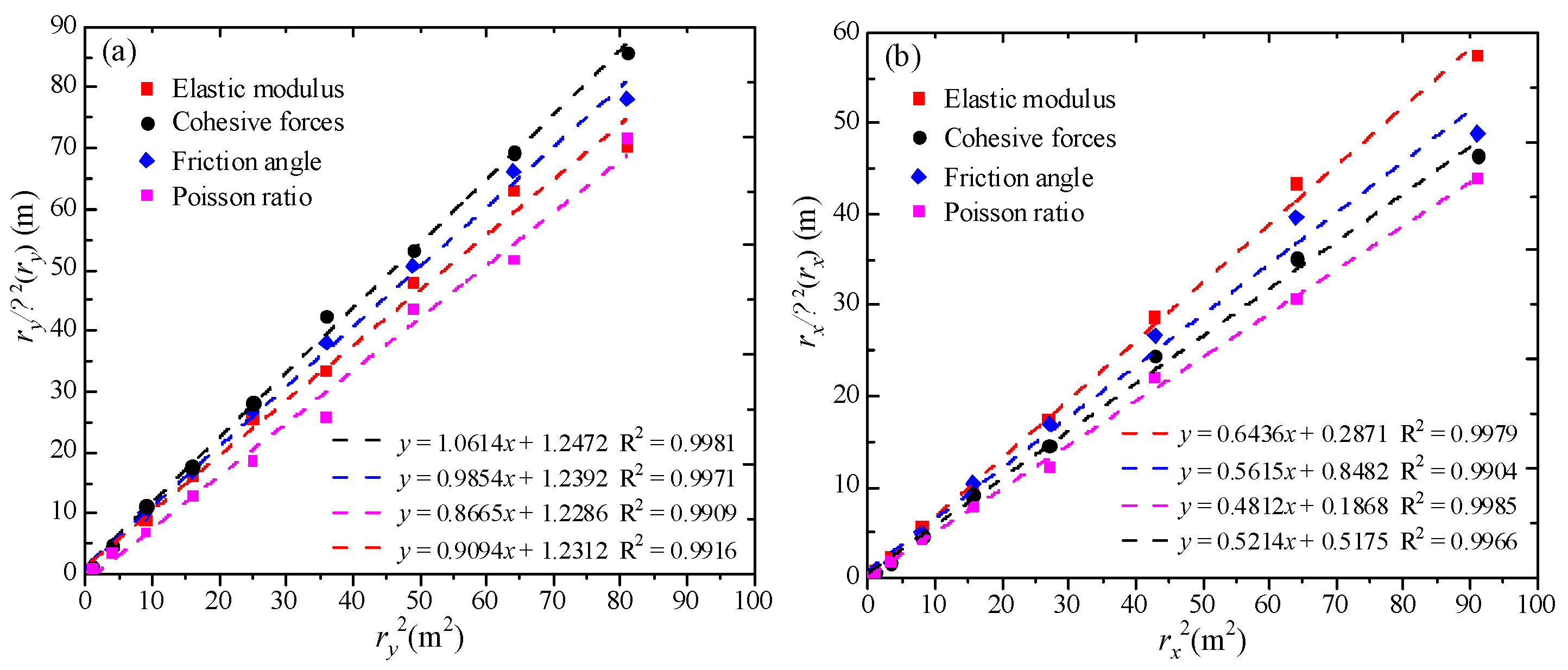
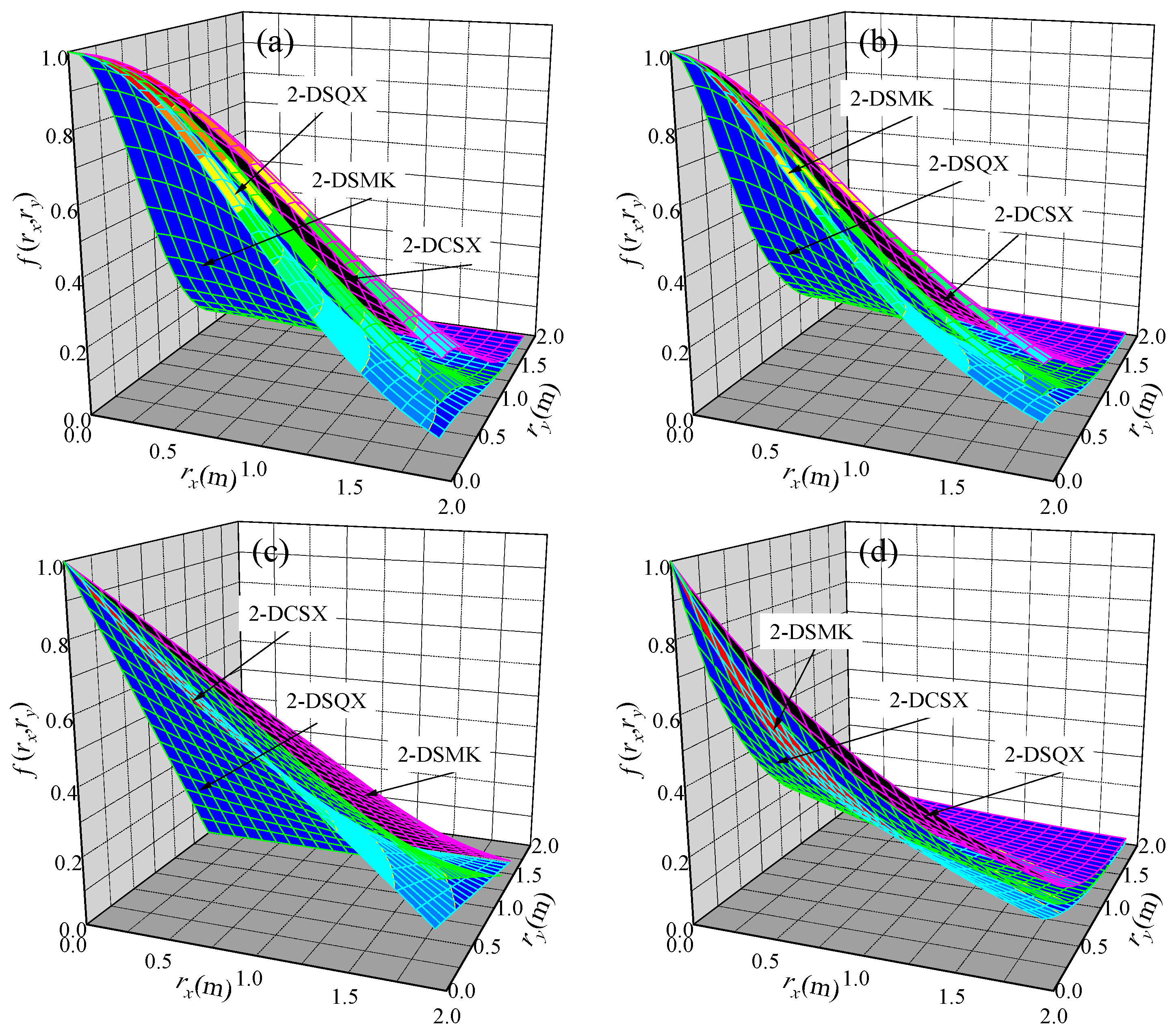
2.2. Spatial Variability Characterization

The heterogeneity leads to non-uniform stress distributions and differential deformations under loading, significantly affecting the ground settlement behavior. In layered or spatially variable strata, softer zones undergo greater compression than that of stiffer layers, resulting in uneven settlement that may damage structures. The relationship between the spatial variability and settlement is influenced by factors such as the correlation length of the soil properties, the layer thickness, and the external loading conditions. Random field theory provides a powerful framework for quantifying the inherent spatial variability of geotechnical materials. The key parameters governing this representation include the mean and standard deviation, which define the central tendency and dispersion of the soil properties. The fluctuation range describes the distance over which the soil properties exhibit significant dependence, reflecting geological deposition patterns. A short correlation length indicates rapid variability, while a longer one suggests more gradual changes [31]. The autocorrelation function mathematically defines how spatial correlation decays with distance. Based on previous studies, the fluctuation range can be determined through regression analysis [32]. Figure 3 presents the fitted curves of the fluctuation scale in the vertical and horizontal directions. Obviously, all four different mechanical parameters can be regressed to linear equations. The linear fitting degrees are all greater than 0.99. Therefore, the linear regression method has sufficient accuracy.

The fluctuation scale in soils describes the spatial persistence of the geotechnical properties, representing the distance over which soil parameters like the strength or compressibility remain correlated. Larger values indicate more homogeneous conditions, while smaller values reflect rapid local variations. This parameter is primarily influenced by the depositional environment, soil type, and stress history. In foundation engineering, the proper characterization of the fluctuation scale is crucial for predicting differential settlement in heterogeneous soils. It directly affects the reliability of settlement predictions and helps optimize foundation design by accounting for natural soil variability. As shown in Figure 3, the abscissa is set as the square of the measured distance, and the ordinate is set as the ratio of the square of the measured distance to the variance reduction function. The reciprocal of the slope is the fluctuation range.

Table 3. Fluctuation scale of geotechnical properties for building foundation soils.

№	Vertical Direction of the Stratum (m)				Horizontal Direction of the Stratum (m)
	EM	PR	CF	FA	EM	PR	CF	FA
1#	1.05	1.20	0.90	0.95	1.45	1.91	1.92	1.61
2#	1.06	1.16	0.97	1.01	1.58	1.96	1.87	1.77
3#	1.13	1.15	0.88	1.04	1.51	2.03	1.99	1.66
4#	1.03	1.15	0.90	1.00	1.47	2.10	2.02	1.72
5#	1.16	1.10	0.92	1.01	1.61	2.10	1.97	1.70
6#	1.15	1.11	0.95	1.02	1.59	1.95	2.18	1.77
7#	1.06	1.15	1.03	1.04	1.54	2.15	1.90	1.87
8#	1.14	1.21	0.95	1.10	1.52	2.12	1.96	1.92
9#	1.17	1.12	0.92	1.12	1.48	2.23	1.73	1.82
10#	1.12	1.24	0.97	1.05	1.41	2.03	1.87	1.73

shows the fluctuation scale of uncertain geotechnical properties in the vertical and horizontal directions. For the vertical fluctuation scale of the four different parameters, the maximum, minimum, and average are 1.24 m, 0.88 m, and 1.06 m, respectively. For the horizontal fluctuation scale of the four different parameters, the maximum, minimum, and average are 2.23 m, 1.41 m, and 1.82 m, respectively. Obviously, the horizontal fluctuation scale is significantly larger than the vertical scale. This phenomenon primarily results from stratified deposition processes during soil formation, where sedimentation creates more continuous horizontal layers compared to vertical profiles. Geological processes like alluvial deposition and weathering further reinforce this directional dependence.

The autocorrelation function (ACF) is a fundamental mathematical tool in soil random field theory that quantifies the spatial dependency of the geotechnical parameters. It describes how the correlation between the soil properties decays with increasing spatial separation distance, reflecting the inherent spatial structure of the soil variability. Common ACF models include the exponential, Gaussian, and spherical functions, each with distinct decay characteristics that correspond to different geological formation processes [33,34]. The proper selection and calibration of the ACF are critical for the accurate simulation of the soil spatial variability, influencing reliability analyses, risk assessment, and geotechnical design optimization in heterogeneous ground conditions. However, it is not known which ACF is better. Therefore, this study selected three of the most common functions and conducted a sensitivity analysis. Namely, the two-dimensional squared exponential (2-DSQX), two-dimensional second-order Markov (2-DSMK), and two-dimensional cosine exponential (2-DCSX) were used to characterize the spatial variability.

Table 4. Characterization functions of spatial variability.

Function Type	Detailed Mathematical Expression	Relationship Between Parameters
2-DSQX	$\rho \left(\tau \right)=\exp \left\{-\left[{\left({\displaystyle \frac{{\tau }_x}{{\theta }_h}}\right)}^2+{\left({\displaystyle \frac{{\tau }_y}{{\theta }_v}}\right)}^2\right]\right\}$	${\theta }_h={\displaystyle \frac{{\delta }_h}{\sqrt{\pi }}},{\theta }_v={\displaystyle \frac{{\delta }_v}{\sqrt{\pi }}}$
2-DSMK	$\rho \left(\tau \right)=\exp \left[-\left({\displaystyle \frac{{\tau }_x}{{\theta }_h}}+{\displaystyle \frac{{\tau }_y}{{\theta }_v}}\right)\right]\left[\left(1+{\displaystyle \frac{{\tau }_x}{{\theta }_h}}\right)\left(1+{\displaystyle \frac{{\tau }_y}{{\theta }_v}}\right)\right]$	${\theta }_h={\displaystyle \frac{{\delta }_h}{4}},{\theta }_v={\displaystyle \frac{{\delta }_v}{4}}$
2-DCSX	$\rho \left(\tau \right)=\exp \left[-\left({\displaystyle \frac{{\tau }_x}{{\theta }_h}}+{\displaystyle \frac{{\tau }_y}{{\theta }_v}}\right)\right]\cos \left({\displaystyle \frac{{\tau }_x}{{\theta }_h}}\right)\cos \left({\displaystyle \frac{{\tau }_y}{{\theta }_v}}\right)$	${\theta }_h={\delta }_h,{\theta }_v={\delta }_v$

Notes: δ and θ are the autocorrelation distance and scale of fluctuation of the soil material, respectively. Subscripts v and h represent the vertical direction and horizontal direction, respectively.

shows the detailed mathematical expressions of the characterization functions. According to Table 3 and Table 4, we can obtain the relationship between the correlation length and fluctuation scale. It can be seen that the different mathematical functions have different parameter relationships.

The ACF in two-dimensional soil random fields exhibits distinct spatial patterns that characterize the soil variability in both the horizontal and vertical directions. When visualized as a 3D surface or contour plot, the ACF typically shows anisotropic behavior, with correlations decaying at different rates along the horizontal (x) and vertical (y) axes. For most natural deposits, the contour lines appear elliptical rather than circular, reflecting stronger spatial continuity horizontally due to layered sedimentation processes. Figure 4 shows the autocorrelation function structure of the spatial variability characterization for uncertain geotechnical properties. It can be seen that different geotechnical parameters have different correlation structures. The most significant difference lies in the rate at which the function graphs change. For the EM and PR, the change within the range of 0.5 m is not significant, but it decreases sharply after exceeding 0.5 m. For the CF and FA, the change is significant within the range of 0.5 m, and the decrease is relatively slow after exceeding 0.5 m.

2.3. Cross-Correlation Characterization

The cross-correlation among the soil parameters represents a fundamental feature in geotechnical engineering, describing the statistical interdependence between the different physical and mechanical properties of soils. These correlations primarily arise from three mechanistic origins: (1) shared geological formation processes, where depositional environments simultaneously control multiple parameters (e.g., the particle size distribution affects both the permeability and shear strength); (2) coupled physical mechanisms, such as the intrinsic relationship between the void ratio and compressibility in consolidation theory; and (3) unified stress history effects, where the past loading conditions jointly influence the current strength and stiffness characteristics. Common correlation patterns involve strong positive correlations between the porosity and permeability in granular soils, moderate negative correlations between the moisture content and undrained shear strength in clay soils, and complex nonlinear dependencies between the friction angle and density in compacted soils. These interdependencies exert a significant influence on geotechnical analyses. For instance, ignoring the natural correlation between the cohesion and friction angle may underestimate failure probabilities by 30–50% [35]. The limited availability of soil parameter samples significantly affects the accuracy and reliability of cross-correlation characterization, primarily through three mechanisms: (1) statistical uncertainty, where small datasets lead to unstable correlation coefficient estimates with standard errors exceeding ±0.2, particularly for non-normal distributed parameters; (2) spurious correlation effects, arising from chance parameter combinations in undersampled strata, which may falsely indicate strong relationships that do not reflect the true geological mechanisms; and (3) truncation bias, where the natural variability range is inadequately captured, distorting the apparent dependence structure between the parameters. Experimental studies show that sample sizes below 15 per soil layer can cause over 40% deviation in estimated correlation coefficients. Copula theory provides a powerful framework for modeling complex dependence structures among geotechnical parameters, overcoming the limitations of traditional correlation coefficients. Unlike conventional methods assuming linear relationships, copulas separate the marginal distributions from the dependence structure, enabling accurate representations of nonlinear and tail dependencies [36]. According to the copula theory, the cross-correlation of any two mechanical parameters in the EM, PR, CF, and FA can be expressed by the following formula:

$$F\left(x_i,x_j\right)=C\left(F_i\left(x_i\right),F_j\left(x_j\right);\theta \right)=C\left(u_i,u_j;\theta \right)$$

(1)

where x_i, x_j are the mechanical parameters of a deep shale reservoir; F(x_i), F(x_j) is the marginal distribution function; and F(x_i, x_j) is the joint distribution function (JDF).

The corresponding probability density function (PDF) can be written as follows:

$$f_{i,j}\left(x_i,x_j\right)=D_{i,j}\left(u_i,u_j;\theta \right)f_i\left(x_i\right)f_j\left(x_j\right)$$

(2)

Table 5. Copula joint distribution functions.

Copula	C(u1,u2; θ)	D(u1,u2; θ)	Range of θ
Gaussian	$\begin{array}{l}C\left(u_1,u_2;\theta \right)={{\displaystyle \int }}_{-\infty }^{{\mathsf{\Phi }}^{-1}\left(u_1\right)}{{\displaystyle \int }}_{-\infty }^{{\mathsf{\Phi }}^{-1}\left(u_2\right)}{\displaystyle \frac{1}{2\pi \sqrt{1-{\theta }^2}}}\hfill \\ \times \exp \left(-{\displaystyle \frac{x_1^2-2\theta x_1{x}_2+x_2^2}{2\left(1-{\theta }^2\right)}}\right)d{x}_1{x}_2\hfill \end{array}$	$\begin{array}{l}D\left(u_1,u_2;\theta \right)={\displaystyle \frac{1}{2\sqrt{1-{\theta }^2}}}\exp \left({\displaystyle \frac{{\varsigma }_1^2-2\theta {\varsigma }_1{\varsigma }_2+{\varsigma }_2^2}{2\left(1-{\theta }^2\right)}}\right)\\ {\varsigma }_1={\mathrm{\Phi }}^{-1}\left(u_1\right),{\varsigma }_2={\mathrm{\Phi }}^{-1}\left(u_2\right)\end{array}$	[−1, 1]
Frank	$-{\displaystyle \frac{1}{\theta }}\ln \left(1+{\displaystyle \frac{\left(e^{-\theta u_1}-1\right)\left(e^{-\theta u_2}-1\right)}{\left(e^{-\theta }-1\right)}}\right)$	${\displaystyle \frac{-\theta \left(e^{-\theta }-1\right)e^{-\theta \left(u_1+u_2\right)}}{{\left[\left(e^{-\theta }-1\right)+\left(e^{-\theta u_1}-1\right)\left(e^{-\theta u_2}-1\right)\right]}^2}}$	$\left(-\infty ,\infty \right)\backslash \left\{0\right\}$
Gumbel	$\exp \left(-{\left({\left(-\ln u_1\right)}^{\theta }+{\left(-\ln u_2\right)}^{\theta }\right)}^{1/\theta }\right)$	$\begin{array}{l}{\displaystyle \frac{e^{-S^{1/\theta }}{\left(\ln u_1\ln u_2\right)}^{\theta -1}\left(S^{1/\theta }+\theta -1\right)}{u_1{u}_2{S}^{2-1/\theta }}}\\ \mathrm{where}S=\left(-\ln u_1\right)\theta +\left(-\ln u_2\right)\theta \end{array}$	$[1,\infty )$
Clayton	${\left(u_1^{-\theta }+u_2^{-\theta }-1\right)}^{-1/\theta }$	$\left(1+\theta \right){(u_1{u}_2)}^{-\theta -1}{\left(u_1^{-\theta }+u_2^{-\theta }-1\right)}^{-2-1/\theta }$	$(0,\infty )$

presents the four detailed copula joint distribution functions. The coefficient τ is defined as follows:

$$\tau ={\displaystyle \frac{{\displaystyle \sum _{i<j}\mathrm{sign}\left[\left(x_{1i}-x_{1j}\right)\left(x_{2i}-x_{2j}\right)\right]}}{0.5N(N-1)}}$$

(3)

where sign [·] is the sign function; x_1i, i = 1,2, ··· N denotes the ith actual value of the parameter X₁; and N denotes the total amount of data.

The relationship between the τ and parameter θ is as follows:

$$\tau =4{\displaystyle {\int }_0^1{\displaystyle {\int }_0^{1}C\left(F_1(x_1),F_2(x_2);\theta \right)}}dC\left(F_1(x_1),F_2(x_2);\theta \right)-1$$

(4)

The bootstrap method is a resampling-based statistical technique used to estimate the uncertainty and distribution characteristics of soil parameters when limited field experiment data are available. Its fundamental principle lies in constructing multiple pseudo-datasets (typically 1000–5000 replicates) by randomly resampling the original observations with replacements. For soil parameter analysis, the procedure involves the following: (1) collecting n field measurements of the target parameter, (2) generating B bootstrap samples by randomly selecting n values with replacements from the original dataset, (3) calculating the statistic of interest (mean, standard deviation, or correlation) for each sample, and (4) determining the confidence intervals from the empirical distribution of these statistics. This non-parametric approach makes no assumptions about the underlying data distribution, making it particularly suitable for skewed geotechnical data like SPT blow counts or undrained shear strengths. Studies show that bootstrap methods can reduce parameter estimation errors by 30–50% compared to conventional Gaussian approximations when sample sizes are small (n < 30). The technique has proven valuable for the stability analysis of uncertain geotechnical properties for variable land subsidence processes, providing robust uncertainty quantification without requiring additional costly field investigations. According to the bootstrap method, the different distributed variables of the EM and PR, CF and FA of uncertain geotechnical properties were simulated. Figure 5 presents the results of the simulation uniformly distributed variables of the cross-correlation characterization for uncertain geotechnical properties. The EM has a negative correlation with the PR, while the CF has a positive correlation with the FA. Figure 6 presents the results of the discrete correlation distribution variables of the cross-correlation characterization for uncertain geotechnical properties. The discrete characteristics of the simulated data have similar discrete characteristics to those of the original data.

Statistical parameters play a crucial role in quantifying the inherent variability in geotechnical soil properties. Key measures include the mean, standard deviation, coefficient of variation, scale of fluctuation (SOF), and autocorrelation distance (ACD). These parameters capture essential characteristics of the soil behavior, such as the strength, compressibility, and permeability, which often exhibit natural randomness due to depositional processes and environmental factors. Understanding these statistical properties is vital for reliability-based design, enabling engineers to account for uncertainty in geotechnical analyses. For instance, the coefficient of variation helps assess risk in the land subsidence stability, while the correlation length influences foundation settlement predictions. Figure 7 shows the statistical characteristics of the simulated geotechnical properties of the soil layer in the investigation area. For the COV, the simulation value is between 0.04 and 0.06. For the SOF, the simulation value is between 1.2 m and 1.7 m. For the ACD, the simulation value is between 0.6 m and 1.2 m.

Table 6. Comparison of statistical properties of field experiment and numerical simulation results.

Statistics	Field Experiment Results				Numerical Simulation Results				Comparative Values
	EM	PR	CF	FA	EM	PR	CF	FA	EM	PR	CF	FA
Sample size	100	100	100	100	1000	1000	1000	1000
Mean (10A MPa)	10.013	0.300	65.585	25.051	9.895	0.297	64.787	25.216	0.118	0.003	0.798	−0.165
SD (10A MPa)	0.502	0.014	2.989	1.424	0.491	0.014	2.987	1.408	0.011	0.000	0.002	0.016
COV	0.050	0.047	0.046	0.057	0.051	0.046	0.045	0.057	−0.001	0.001	0.001	0.000
Max (10A MPa)	11.366	0.337	71.815	28.687	11.307	0.333	70.846	28.612	0.059	0.004	0.969	0.075
Min (10A MPa)	8.678	0.266	58.617	21.214	8.707	0.263	58.464	20.957	−0.029	0.003	0.153	0.257
Skewness	−0.113	−0.292	−0.074	−0.055	−0.113	−0.296	−0.074	−0.055	0.000	0.004	0.000	0.000
Peakedness	0.106	−0.074	−0.649	−0.300	0.106	−0.074	−0.650	−0.303	0.000	0.000	0.001	0.003

Notes: A = 1 when the statistics are the EM; A = −3 when the statistics are the CF.

presents a comparison of the field experiment and numerical simulation results. The statistics of the simulated data and the test data are basically the same. Bootstrap-simulated data are derived through random resampling (with replacement) from the original dataset, preserving its statistical properties while enabling uncertainty quantification. Each bootstrap sample mirrors the original data’s distribution but introduces controlled variability to assess the parameter robustness. The method generates multiple synthetic datasets to construct confidence intervals for key parameters (mean, variance). Crucially, bootstrap data maintain the original sample’s correlation structure and spatial trends, making them ideal for small-sample geotechnical problems. This approach circumvents parametric assumptions, utilizing empirical data to enhance the reliability in variable land subsidence analyses.

3. Uncertainty Analysis of Building Foundation Soils

3.1. Mathematical Equations and Elastoplastic Method

The constitutive relationship of soils, which describes the stress–strain behavior under loading, fundamentally governs the magnitude and pattern of ground settlement. Different constitutive models (e.g., linear elastic, elastoplastic, or critical-state models) capture varying soil responses—elastic compression, plastic yielding, or time-dependent creep—each contributing uniquely to settlement. For instance, the Modified Cam-Clay model effectively predicts the long-term consolidation settlement in clays by incorporating the void ratio and effective stress interactions, while nonlinear elastic models better represent granular soils’ immediate settlement. The choice of constitutive model directly impacts settlement predictions: oversimplified models (e.g., linear elasticity) may underestimate the differential settlement by 20–40%, whereas advanced models accounting for the soil anisotropy and small-strain stiffness improve accuracy. In layered strata, coupling constitutive laws with spatial variability parameters (e.g., fluctuation scales) enables the precise simulation of uneven settlement. The Modified Cam-Clay model is a critical-state-based elastoplastic constitutive model that accurately describes the mechanical behavior of cohesive soils. It introduces an elliptical yield surface in the p–q stress space (where p is the mean effective stress and q is the deviatoric stress), which evolves through isotropic hardening/softening based on the plastic volumetric strains. Its key strength lies in simultaneously predicting both shear failure (through the critical state concept) and consolidation behavior, including pore pressure development and stress path dependency [37,38]. The model effectively captures the pressure-dependent stiffness and strength characteristics of clays, making it invaluable for analyzing variable land subsidence processes. However, it has limitations in modeling granular soils, small-strain nonlinearity, and anisotropic conditions. Therefore, this study developed a dual-yield surface constitutive model to characterize the geotechnical properties of soil layers. This model adopts a stress path-dependent factor to modify the yield surface hardening parameters obtained from the isotropic consolidation path, yielding stress path-independent current yield surface hardening parameters. Via the combination with critical-state parameters, reference yield surface hardening parameters that can reflect the inherent critical characteristics of soil are derived. A self-developed program is implemented to realize the prediction function of the established constitutive model. The yield function can be written as follows:

$$f=\ln {\displaystyle \frac{p}{p_0}}+\ln \left(1+{\displaystyle \frac{q^2}{M^{2}p\left(p+p_r\right)}}\right)-{\displaystyle \int \frac{d{\epsilon }_v^p}{{\phi }^{\prime }\left(\ln p\right)-\kappa }}=0$$

(5)

$$q={\displaystyle \frac{6\sin \phi }{3-\sin \phi }}p+{\displaystyle \frac{6\cos \phi }{3-\sin \phi }}c$$

(6)

$$M={\displaystyle \frac{6\sin \phi }{3-\sin \phi }};p_r=c\cot \phi$$

(7)

where $\phi$ and $c$ are the FA and CF of the soil material, respectively; ${\phi }^{\prime }$ and $\kappa$ are the isotropic consolidation curve and rebound slope, respectively.

Under loading, soils typically exhibit three phases: initial elastic deformation, plastic yielding, and failure. Cohesive soils show strain softening post-peak strength, while granular soils often demonstrate strain hardening. Key characteristics include pressure-dependent stiffness, dilatancy effects, and critical-state behavior at large strains. Our dual-yield surface constitutive model can respond to strain softening and strain hardening. The elastic matrix can be expressed as follows:

$${\left[C\right]}^e=\left[\begin{array}{cccccc}\left(K+{\displaystyle \frac{4}{3}}G\right)& \left(K-{\displaystyle \frac{2}{3}}G\right)& \left(K-{\displaystyle \frac{2}{3}}G\right)& 0& 0& 0\\ \left(K-{\displaystyle \frac{2}{3}}G\right)& \left(K+{\displaystyle \frac{4}{3}}G\right)& \left(K-{\displaystyle \frac{2}{3}}G\right)& 0& 0& 0\\ \left(K-{\displaystyle \frac{2}{3}}G\right)& \left(K-{\displaystyle \frac{2}{3}}G\right)& \left(K+{\displaystyle \frac{4}{3}}G\right)& 0& 0& 0\\ 0& 0& 0& G& 0& 0\\ 0& 0& 0& 0& G& 0\\ 0& 0& 0& 0& 0& G\end{array}\right]$$

(8)

$$K={\displaystyle \frac{dp}{d{\epsilon }_v^e}}={\displaystyle \frac{E}{3\left(1-2v\right)}}={\displaystyle \frac{p}{\kappa }}$$

(9)

$$G={\displaystyle \frac{dq}{3d{\epsilon }_d^e}}={\displaystyle \frac{E}{2\left(1+v\right)}}={\displaystyle \frac{3\left(1-2v\right)}{2\left(1+v\right)}}K$$

(10)

where E and v are the EM and PR of the soil material, respectively.

The classical elastoplastic theory describes materials that exhibit reversible elastic deformation and irreversible plastic flow. It combines Hooke’s law for elasticity with three plasticity components: (1) a yield criterion defining the elastic limit, (2) a flow rule governing the plastic strain direction, and (3) a hardening law tracking the yield surface evolution. The theory decomposes the strain into elastic and plastic parts, enabling the prediction of permanent deformation in metals, soils, and polymers under loading–unloading cycles. The total strain increment can be expressed as follows:

$$d{\sigma }_{ij}=C_{ijkl}^{e}d{\epsilon }_{kl}^e=C_{ijkl}^e\left(d{\epsilon }_{kl}-d{\epsilon }_{kl}^p\right)$$

(11)

The increment of plastic strain is determined by the plastic potential theory:

$$d{\epsilon }_{ij}^p=d\lambda {\displaystyle \frac{\partial g}{\partial {\sigma }_{ij}}}$$

(12)

$$d\lambda ={\displaystyle \frac{\frac{\partial f}{\partial {\sigma }_{ij}}{C}_{ijkl}^{e}d{\epsilon }_{kl}}{-\frac{\partial f}{\partial H}\frac{\partial H}{\partial {\epsilon }_{ij}^p}\frac{\partial g}{\partial {\sigma }_{ij}}+\frac{\partial f}{\partial {\sigma }_{ij}}{C}_{ijkl}^e\frac{\partial g}{\partial {\sigma }_{kl}}}}$$

(13)

$$C_{ijkl}^{ep}=C_{ijkl}^e-{\displaystyle \frac{C_{ijmn}^e\frac{\partial g}{\partial {\sigma }_{mn}}\frac{\partial f}{\partial {\sigma }_{st}}{C}_{stkl}^e}{A+\frac{\partial f}{\partial {\sigma }_{ij}}{C}_{ijkl}^e\frac{\partial g}{\partial {\sigma }_{kl}}}}$$

(14)

where H is the yield surface hardening parameter.

By adopting the applicable flow rule, where the yield function equals the plastic potential function, the differential equation can be expressed as follows:

$${\displaystyle \frac{\partial f}{\partial \sigma }}={\displaystyle \frac{\partial f}{\partial I_1}}{\displaystyle \frac{\partial I_1}{\partial \sigma }}+\left[{\displaystyle \frac{\partial f}{\partial \sqrt{J_2}}}+{\displaystyle \frac{\partial f}{\partial \theta }}{\displaystyle \frac{\cot 3\theta }{\sqrt{J_2}}}\right]{\displaystyle \frac{\partial \sqrt{J_2}}{\partial \sigma }}+{\displaystyle \frac{\partial f}{\partial \theta }}{\displaystyle \frac{\sqrt{3}}{2sin3\theta }}{\displaystyle \frac{1}{{\left(J_2\right)}^{3/2}}}{\displaystyle \frac{\partial J_3}{\partial \sigma }}$$

(15)

$${\displaystyle \frac{\partial I_1}{\partial \sigma }}=\left[\begin{array}{l}1\\ 1\\ 1\\ 0\\ 0\\ 0\end{array}\right],{\displaystyle \frac{\partial I_2}{\partial \sigma }}=\left[\begin{array}{c}{\sigma }_{22}+{\sigma }_{33}\\ {\sigma }_{11}+{\sigma }_{33}\\ {\sigma }_{11}+{\sigma }_{22}\\ -2{\sigma }_{12}\\ -2{\sigma }_{23}\\ -2{\sigma }_{13}\end{array}\right],{\displaystyle \frac{\partial I_3}{\partial \sigma }}=\left[\begin{array}{c}{\sigma }_{22}{\sigma }_{33}-{\sigma }_{23}^2\\ {\sigma }_{11}{\sigma }_{33}-{\sigma }_{13}^2\\ {\sigma }_{11}{\sigma }_{22}-{\sigma }_{12}^2\\ 2\left({\sigma }_{23}{\sigma }_{13}-{\sigma }_{33}{\sigma }_{12}\right)\\ 2\left({\sigma }_{12}{\sigma }_{13}-{\sigma }_{11}{\sigma }_{23}\right)\\ 2\left({\sigma }_{12}{\sigma }_{23}-{\sigma }_{22}{\sigma }_{13}\right)\end{array}\right]$$

(16)

$${\displaystyle \frac{\partial J_1}{\partial \sigma }}=\left[\begin{array}{l}1\\ 1\\ 1\\ 0\\ 0\\ 0\end{array}\right],{\displaystyle \frac{\partial J_2}{\partial \sigma }}=\left[\begin{array}{c}{\displaystyle \frac{2}{3}}{I}_1-\left({\sigma }_{22}+{\sigma }_{33}\right)\\ {\displaystyle \frac{2}{3}}{I}_1-\left({\sigma }_{11}+{\sigma }_{33}\right)\\ {\displaystyle \frac{2}{3}}{I}_1-\left({\sigma }_{11}+{\sigma }_{22}\right)\\ 2{\sigma }_{12}\\ 2{\sigma }_{23}\\ 2{\sigma }_{13}\end{array}\right],{\displaystyle \frac{\partial J_3}{\partial \sigma }}=\left[\begin{array}{c}\left({\displaystyle \frac{2}{9}}{I}_1^2-{\displaystyle \frac{1}{3}}{I}_2\right)+\left({\sigma }_{22}+{\sigma }_{33}\right)\left(-{\displaystyle \frac{1}{3}}{I}_1\right)+\left({\sigma }_{22}{\sigma }_{33}-{\sigma }_{23}^2\right)\\ \left({\displaystyle \frac{2}{9}}{I}_1^2-{\displaystyle \frac{1}{3}}{I}_2\right)+\left({\sigma }_{11}+{\sigma }_{33}\right)\left(-{\displaystyle \frac{1}{3}}{I}_1\right)+\left({\sigma }_{11}{\sigma }_{33}-{\sigma }_{13}^2\right)\\ \left({\displaystyle \frac{2}{9}}{I}_1^2-{\displaystyle \frac{1}{3}}{I}_2\right)+\left({\sigma }_{11}+{\sigma }_{22}\right)\left(-{\displaystyle \frac{1}{3}}{I}_1\right)+\left({\sigma }_{11}{\sigma }_{22}-{\sigma }_{12}^2\right)\\ \left(2{\sigma }_{23}{\sigma }_{13}-2{\sigma }_{33}{\sigma }_{12}\right)+\left({\displaystyle \frac{2{\sigma }_{12}}{3}}{I}_1\right)\\ \left(2{\sigma }_{12}{\sigma }_{13}-2{\sigma }_{11}{\sigma }_{23}\right)+\left({\displaystyle \frac{2{\sigma }_{23}}{3}}{I}_1\right)\\ \left(2{\sigma }_{12}{\sigma }_{23}-2{\sigma }_{22}{\sigma }_{13}\right)+\left({\displaystyle \frac{2{\sigma }_{13}}{3}}{I}_1\right)\end{array}\right]$$

(17)

To facilitate the code writing of the variable land subsidence processes, the product of the first-order derivative of any stress component of the yield function (f) can obtain the following matrix-form expression:

$${}^{-}{\left[C\right]}^e\left[{\displaystyle \frac{\partial f}{\partial \sigma }}\right]={\left[C\right]}^e\left[{\displaystyle \frac{\partial g}{\partial \sigma }}\right]=\left[\begin{array}{c}\left(K+{\displaystyle \frac{4}{3}}G\right){\displaystyle \frac{\partial f}{\partial {\sigma }_{11}}}+\left(K-{\displaystyle \frac{2}{3}}G\right){\displaystyle \frac{\partial f}{\partial {\sigma }_{22}}}\\ \left(K-{\displaystyle \frac{2}{3}}G\right){\displaystyle \frac{\partial f}{\partial {\sigma }_{11}}}+\left(K+{\displaystyle \frac{4}{3}}G\right){\displaystyle \frac{\partial f}{\partial {\sigma }_{22}}}\\ G{\displaystyle \frac{\partial f}{\partial {\sigma }_{12}}}\end{array}\right]$$

(18)

According to Equations (11)–(18), the stress increment can be obtained. Based on the incremental of the stress–strain relationship and the variable stiffness elastoplastic finite element algorithm, the variable land subsidence processes can be calculated.

3.2. Uncertainty Analysis Method of Settlement

The stochastic finite element method is a computational approach that evaluates ground deformation while considering the natural variability in soil and rock properties. It combines traditional finite element analysis with statistical techniques to model how uncertainties in material parameters influence deformation patterns. The process begins by representing the key geotechnical properties as spatially varying random fields, which capture the measured trends and variability from site investigations [39,40]. Multiple finite element simulations are then performed, each with different realizations of the random property fields, to generate a range of possible deformation outcomes. The statistical analysis of these results provides probabilistic insights, such as the likelihood of exceeding critical settlement thresholds or the expected range of differential displacements. This method evaluates soil deformation by accounting for the natural variability in geotechnical properties. The process begins with site investigation data to determine the statistical characteristics of the soil parameters. Next, multiple realistic soil property fields are generated through random field simulation, capturing spatial variations. Each property field serves as input for a standard finite element analysis, solving equilibrium equations to compute deformations under applied loads. Hundreds of such simulations create a dataset of possible deformation outcomes. Finally, statistical analysis extracts key insights, including probable settlement ranges and the risk of exceeding the design limits.

The EM, PR, CF, and FA of uncertain geotechnical properties for variable land subsidence processes are simulated as random fields. The unit mode is expressed as follows:

$$X_e={\displaystyle \frac{1}{A_e}}{\displaystyle {\int }_{{\mathrm{\Omega }}_e}X(x,y)dxdy}$$

(19)

where A_e represents the area of e (m²); Ω_e represents the integral area of e (m²); and X (x, y) represents the random field.

The covariance can be expressed as follows:

$$Cov(X_e,X_{e^{\prime }})={\displaystyle \frac{{\sigma }^2}{A_e{A}_{e^{\prime }}}}{\displaystyle {\int }_{{\mathrm{\Omega }}_e}{\displaystyle {\int }_{{\mathrm{\Omega }}_{e^{\prime }}}\rho \left(\tau \right)dAd{A}^{\prime }}}={\displaystyle \frac{{\sigma }^2}{A_e{A}_{e^{\prime }}}}{\displaystyle {\int }_{{\mathrm{\Omega }}_e}{\displaystyle {\int }_{{\mathrm{\Omega }}_{e^{\prime }}}\rho (x-x^{\prime },y-y^{\prime })dxd{x}^{\prime }dyd{y}^{\prime }}}$$

(20)

According to the coordinate transformation, x, y, x′, and y′ can be written as follows:

$$x={\displaystyle \sum _{i=1}^4{f}_i{x}_i};y={\displaystyle \sum _{i=1}^4{f}_i{y}_i};x^{\prime }={\displaystyle \sum _{i=1}^4{f}_i^{\prime }{x}_i^{\prime }};y^{\prime }={\displaystyle \sum _{i=1}^4{f}_i^{\prime }{y}_i^{\prime }}$$

(21)

where

$$f_i=\left\{\begin{array}{l}{\displaystyle \frac{1}{4}}(1+{\xi }_i\xi )(1+{\eta }_i\eta )({\xi }_i\xi +{\eta }_i\eta -1)i=1,2,3,4\\ {\displaystyle \frac{1}{2}}(1-{\xi }^2)(1+{\eta }_i\eta )i=5,7\\ {\displaystyle \frac{1}{2}}(1+{\xi }_i\xi )(1-{\eta }^2)i=6,8\end{array}\right.$$

(22)

$${f^{\prime }}_i=\left\{\begin{array}{l}{\displaystyle \frac{1}{4}}(1+{{\xi }^{\prime }}_i{\xi }^{\prime })(1+{{\eta }^{\prime }}_i{\eta }^{\prime })({{\xi }^{\prime }}_i{\xi }^{\prime }+{{\eta }^{\prime }}_i{\eta }^{\prime }-1)i=1,2,3,4\\ {\displaystyle \frac{1}{2}}(1-{{\xi }^{\prime }}^2)(1+{{\eta }^{\prime }}_i{\eta }^{\prime })i=5,7\\ {\displaystyle \frac{1}{2}}(1+{{\xi }^{\prime }}_i{\xi }^{\prime })(1-{{\eta }^{\prime }}^2)i=6,8\end{array}\right.$$

(23)

$$\left\{\begin{array}{l}{\xi }_k={\xi }_k^{\prime }=-1k=1,4,8\\ {\xi }_l={\xi }_l^{\prime }=1l=2,3,6\\ {\xi }_m={\xi }_m^{\prime }=0k=5,7\end{array}\right.$$

(24)

$$\left\{\begin{array}{l}{\eta }_k={\eta }_k^{\prime }=-1k=1,2,5\\ {\eta }_l={\eta }_l^{\prime }=1l=3,4,7\\ {\eta }_m={\eta }_m^{\prime }=0l=6,8\end{array}\right.$$

(25)

According to Equation (20), the covariance matrix can be obtained, and then the random finite element calculation of the uncertain geotechnical properties for the variable land subsidence processes can be carried out. This combined approach begins by characterizing the spatial variability in the soil properties through random field modeling, which transforms site investigation data into statistically representative property distributions. The generated random fields are then discretized and mapped onto finite element meshes, assigning distinct material parameters to each element while preserving spatial correlations. Multiple finite element analyses are performed using different realizations of these randomized property fields to simulate potential deformation patterns. The ensemble results undergo statistical processing to quantify deformation uncertainties, identifying critical variability patterns and their engineering impacts. This integrated methodology enables the probabilistic assessment of geotechnical behavior while maintaining computational efficiency through optimized sampling techniques. The combined approach provides a powerful tool for risk-based design by simultaneously capturing the material variability and mechanical response in geotechnical systems.

3.3. Workflow of Proposed Framework

The stability analysis of the uncertain geotechnical properties for variable land subsidence processes involves obtaining the statistical characteristics of the soil layers; the variability in the uncertain geotechnical properties, characterized by random fields; the cross-correlation of the soil layer under incomplete probabilistic information, characterized by the copula method; mathematical equations and the elastoplastic method of the stress–strain relationship of the soil mass; and the uncertainty analysis method of random finite elements and random fields for the variable land subsidence processes. In detail, the workflows of the proposed framework need five steps:

(1)

Standard testing procedures to evaluate the soil properties through field and laboratory methods, including sampling, penetration tests, and triaxial compression tests. Statistical analysis processes the measured data to determine the central trends, variability ranges, and spatial correlation patterns.

(2)

Quantifying the soil variability using spatial random fields involves analyzing how the soil properties change across locations. This method treats the soil characteristics as continuous random variables, capturing their spatial patterns and correlations.

(3)

Copula methods quantify the statistical dependence in the soil properties by modeling their joint distributions without assuming linear relationships. They capture complex correlations between different soil parameters, such as the EM, PR, CF, and FA, using flexible multivariate frameworks.

(4)

The variable stiffness elastoplastic method for soil deformation considers how the soil stiffness changes under loading. It combines elastic and plastic behaviors, adjusting the stiffness based on stress levels to better simulate real-world soil responses. Through the incremental stress–strain relationship and considering the load step, the deformation characteristics are calculated by self-programming.

(5)

Stochastic finite element analysis for soils involves modeling the spatial variability through random field generation, discretizing it into finite elements, and performing Monte Carlo simulations to compute probabilistic structural responses. This method efficiently quantifies the uncertainty in geotechnical behavior under varying conditions.

4. Risk Assessment of Variable Settlement Properties

4.1. Distribution Fitting Test

The distribution fitting test for soil settlement calculation results involves a systematic process to evaluate how well the computed deformation data align with the theoretical probability distributions. Initially, the settlement values obtained from numerical simulations or field measurements are organized into a dataset, which is then visualized using histograms or probability plots to identify potential distribution patterns. Common candidate distributions such as normal, log-normal, or Weibull distributions are selected based on the data characteristics. Statistical goodness-of-fit tests are then applied to quantify the agreement between the empirical data and each theoretical distribution. These tests typically compare the observed frequencies with the expected frequencies under the hypothesized distribution, generating metrics that indicate the level of fit [41]. Aimed at the boundary values of the stratum settlement characteristics across different moments, while analyzing the probability model of mechanical state variables and grounded in the fundamental principles of the limit-state equation, random numbers are substituted into the state function to generate random values of the state function. N random numbers of state functions are generated in the same way. The sample convergence criterion can be expressed as follows:

$$\underset{N\to \infty }{\lim }P\left(\left|{\displaystyle \frac{1}{n}}\sum _{i=1}^n{X}_i-\mu \right|<\epsilon \right)=1$$

(26)

where $X_1,\hspace{0.33em}{X}_2,\hspace{0.33em}\cdots ,\hspace{0.33em}{X}_n,\cdots$ are the uncertain geotechnical properties for the variable land subsidence processes in different locations.

The probability convergence criterion can be expressed as follows:

$$\underset{N\to \infty }{\lim }P\left(\left|{\displaystyle \frac{n}{N}}-P(A)\right|<\epsilon \right)=1$$

(27)

According to Equations (26) and (27), the settlement data of different regions can be grouped. The analysis process of the law of large numbers in soil settlement deformation involves collecting extensive settlement data from field measurements or numerical simulations. As the sample size grows, statistical averaging reveals stable deformation trends, filtering out local irregularities caused by soil heterogeneity. The probabilistic models can be verified by comparing multiple datasets to observe convergence in settlement behavior. This approach reduces the uncertainty, enhances the prediction reliability, and supports data-driven decisions in geotechnical design by demonstrating that aggregated results increasingly reflect the true underlying deformation mechanisms. The process underscores the importance of sufficient data volumes for accurate settlement characterization.

4.2. Failure Probability

The assessment of the failure probability in ground settlement plays a critical role in engineering safety. Excessive settlement probability may lead to structural damage, pipeline fractures, or the functional failure of infrastructure, particularly in soft-soil regions or high-fill projects. Numerical models such as the finite element or finite difference methods are then employed to simulate settlement responses under various conditions using probabilistic parameter inputs. Reliability analysis techniques, including Monte Carlo sampling or response surface methods, calculate the likelihood of settlements exceeding design thresholds. Modern approaches incorporate Bayesian updating to dynamically refine probability models with real-time monitoring data during construction, significantly improving the prediction accuracy [42,43]. This probabilistic framework supports risk-informed decision making for differential foundation treatments, insurance cost estimation, and lifecycle risk management, proving particularly valuable for critical infrastructure like high-speed railways and oil storage facilities where uneven settlement carries severe consequences. The acceptable range for soil settlement failure probability varies significantly based on the project requirements and risk tolerance. For critical infrastructure like bridges or high-rise buildings, the allowable probability typically remains below five percent to ensure strict safety standards. In less sensitive structures or temporary constructions, probabilities up to ten percent may be deemed acceptable. The specific threshold depends on factors like the potential damage severity, economic consequences, and repair feasibility. Based on the variable land subsidence processes and reliability index, the failure probability can be written as follows:

$$P_f=1-\beta =1-p\left\{F_X\left(X_1,X_2,\cdot \cdot \cdot ,X_n\right)-S\le 0\right\}={\displaystyle \frac{n}{N}}$$

(28)

Therefore, according to the test procedure and statistical characteristics, spatial variability characterization, cross-correlation characterization, mathematical equations and elastoplastic method, and the uncertainty analysis method of settlement, the variable land subsidence can be analyzed and predicted.

5. Results and Analyses

5.1. Validation of Uncertainty Stability Analysis Model

Validating numerical models for ground settlement is essential to ensure their reliability in predicting real-world soil behavior. The validation process involves comparing simulated settlements with field measurements, laboratory test data, or benchmark case studies to verify the model’s ability to capture key mechanisms like consolidation, creep, and stress redistribution. This critical step helps identify the modeling limitations, refine the input parameters, and improve the representation of the soil stratification and material properties. For infrastructure projects involving sensitive structures or compressible soils, thorough validation becomes particularly important to prevent serviceability failures caused by differential settlement. By establishing model credibility through systematic verification, it can make informed decisions about variable land subsidence while accounting for geological uncertainties. Proper validation ultimately bridges the gap between theoretical simulations and actual ground responses. Figure 8a show the comparison of the measurement results and calculation results for the average settlement in three different investigation areas. The stratum settlement increased relatively rapidly in the first two months and relatively slowly in the following two months. The rates of increase at the three positions are different, but the final settlement amounts are basically the same (approximately 22.5 mm). It can be seen that the test results of the mean settlement are basically the same as the simulation results. Figure 8b shows the comparison of the measurement results and calculation results for the standard deviation in three different investigation areas. The standard deviation increases first and then decreases. The maximum standard deviation is between 1.5 mm and 2.0 mm. It can be seen that the test results of the standard deviation are basically the same as the simulation results. Therefore, the stability analysis method for uncertain geotechnical properties for variable land subsidence processes in this paper is scientific and reasonable.

5.2. Stability Indicators at Different Locations

Distributed fitting tests for ground settlement analysis involve evaluating how well field-measured deformation data match theoretical distribution patterns across spatial domains. This method examines the settlement uniformity by comparing multi-point monitoring results with expected probability distributions through statistical techniques. We collected dense settlement measurements across the affected areas and then analyzed their spatial correlations and distribution characteristics using both visual probability plots and quantitative statistical tests. This distributed analysis proves particularly valuable for variable land subsidence processes, where the spatial variability significantly impacts the structural performance. The fitting results guide reliability assessments and inform targeted ground improvement strategies, ensuring that the statistical model properly represents the actual deformation behavior throughout the entire influence zone rather than at isolated points. This comprehensive approach enhances the prediction accuracy for settlement impacts. Taking investigation area #1 as an example,

Table 7. Frequency distribution of variable settlement for investigation area #1.

№	Group (ti−1, ti]	Absolute Frequency, fi	Frequency, fi/n	Cumulative Frequency
1	[11.776, 12.930]	15	0.0015	0.0650
2	(12.930, 14.084]	121	0.0121
3	(14.084, 15.238]	619	0.0619
4	(15.238, 16.392]	1902	0.1902	0.2141
5	(16.392, 17.546]	3011	0.3011	0.489
6	(17.546, 18.701]	2649	0.2649	0.7693
7	(18.701, 19.855]	1314	0.1314	0.9313
8	(19.855, 21.009]	316	0.0316	0.9313 + 0.0687 = 1
9	(21.009, 22.163]	47	0.0047
10	(22.163, 23.317]	6	0.0006

presents the frequency distribution of the variable land subsidence after 10,000 simulations. The sample data can be divided into 10 groups. The maximum settlement is 23.317 mm, while the minimum settlement is 11.776 MPa.

Further combining the frequencies less than 0.05, six interval ranges can be obtained, which are (−∞, 15.238], (15.238, 16.392], (16.392, 17.546], (17.546, 18.701], (18.701, 19.855], and (19.855, +∞]. The frequency is as follows:

$$p_i=\mathrm{\Phi }\left({\displaystyle \frac{t_i-\mu }{\sigma }}\right)-\mathrm{\Phi }\left({\displaystyle \frac{t_{i-1}-\mu }{\sigma }}\right)$$

(29)

The chi-square distributions (χ²) are shown in

Table 8. Computation sheet (χ²) of variable settlement for investigation area #1.

№	Group (ti−1, ti]	Absolute Frequency, fi	Frequency, pi	npi	(fi−npi)2/npi
1	(−∞, 15.238]	755	0.0769	769.00	0.2549
2	(15.238, 16.392]	1902	0.1898	1898.00	0.0084
3	(16.392, 17.546]	3011	0.3050	3050.00	0.4987
4	(17.546, 18.701]	2649	0.2658	2658.00	0.0305
5	(18.701, 19.855]	1314	0.1256	1256.00	2.6783
6	(19.855, +∞]	369	0.0376	376.00	0.1303
Total		10,000	1.0000	10,000	3.6011

.

From Table 8, χ² = 3.6011 and χ²_0.10 (3) = 6.251. It is obvious that χ² < χ²_0.10 (3). Therefore, the variable land subsidence for investigation area #1 follows a normal distribution with a significance level of 0.1.

5.3. Impact of Spatial Variation on Building Settlement

Figure 9 shows the failure probability of variable stratum settlement for different spatial variations of geotechnical properties. For investigation area #1, the maximum is 6.68% while the minimum is 3.88%. The means of the 2-DSQX, 2-DSMK, and 2-DCSX of uncertain geotechnical properties are 3.76%, 3.93%, and 3.84%. This indicates that the influence of the variability parameter in investigation area #1 is greater than that of the correlation structure. For investigation area #2, the maximum is 6.26%, while the minimum is 4.11%. The means of the 2-DSQX, 2-DSMK, and 2-DCSX of uncertain geotechnical properties are 4.32%, 3.73%, and 4.14%. This indicates that the influence of the variability parameter in investigation area #2 is greater than that of the correlation structure. For investigation area #3, the maximum is 6.68%, while the minimum is 4.06%. The means of the 2-DSQX, 2-DSMK, and 2-DCSX of uncertain geotechnical properties are 4.06%, 4.41%, and 4.20%. This indicates that the influence of the variability parameter in investigation area #3 is smaller than that of the correlation structure. In fact, the correlation structure within soil random fields fundamentally influences the ground settlement mechanisms through the spatial interdependence of the geotechnical parameters. This inherent connectivity dictates how localized deformation propagates across geological formations, creating complex settlement patterns that deviate from uniform predictions. Strong horizontal correlations in cohesive layers typically produce widespread, bowl-shaped subsidence, while weak vertical correlations in granular soils often lead to irregular differential settlement. The spatial decay characteristics determine whether the settlement effects remain concentrated near loading zones or extend progressively across wider areas. The correlation range directly controls the effective influence radius of the soil variability, with longer ranges amplifying settlement uncertainties across larger volumes. Understanding these mechanisms enables more accurate reliability assessments by accounting for spatially coordinated soil behavior rather than treating properties as isolated variables. The correlation structure ultimately governs how heterogeneous soil systems collectively respond to loading, making its proper characterization essential for predicting realistic settlement distributions in variable ground conditions.

5.4. Impact of Cross-Correlation on Building Settlement

Figure 10 shows the failure probabilities of variable stratum settlement for different cross-correlations of geotechnical properties under positive copula conditions. For investigation area #1, with the increase in the correlation coefficient, the failure probabilities of the Gaussian Copula, Frank Copula, and Gumbel Copula gradually decrease, and the failure probability of the Clayton Copula first decreases and then increases. When using the Clayton Copula to characterize the cross-correlation of the geotechnical properties, the failure probability is higher. The maximum is 7.59%, while the minimum is 4.94%. When using the Gaussian Copula to characterize the cross-correlation of the geotechnical properties, the failure probability is smaller. The minimum is 2.64%, while the maximum is 5.01%. For investigation area #2, with the increase in the correlation coefficient, the failure probabilities of three copula functions gradually decrease, and the failure probability of the Clayton Copula is basically stable. When using the Clayton Copula to characterize the cross-correlation of geotechnical properties, the failure probability is higher. The maximum is 6.45%, while the minimum is 5.36%. When using the Gaussian Copula to characterize the cross-correlation of geotechnical properties, the failure probability is smaller. The minimum is 2.56%, while the maximum is 4.65%. For investigation area #3, with the increase in the correlation coefficient, the failure probabilities of three copula functions gradually decrease, and the failure probability of the Clayton Copula is basically stable. When using the Clayton Copula to characterize the cross-correlation of the geotechnical properties, the failure probability is higher. The maximum is 5.70%, while the minimum is 4.01%. When using the Gaussian Copula to characterize the cross-correlation of the geotechnical properties, the failure probability is smaller. The minimum is 2.38%, while the maximum is 3.97%. Different cross-correlation structures have different influences on the failure probability of variable stratum settlement. In fact, the positive correlation among the soil mechanical parameters profoundly impacts ground settlement mechanisms by synchronizing adverse material behaviors across the influence zone. When the strength and stiffness parameters vary coherently, weak compressible regions tend to cluster spatially, creating concentrated deformation zones instead of dispersing settlement evenly. This aligned variability leads to cascading effects wherein localized yielding triggers progressive stress redistribution, amplifying settlement accumulation in vulnerable areas. In stratified soils, positively correlated layers develop coordinated compression patterns, potentially generating bowl-shaped subsidence profiles with sharper edges. The phenomenon becomes particularly significant under foundation loads, where synchronized softening in adjacent soil volumes reduces the load-transfer efficiency, increasing the total settlement magnitude. Such correlation-driven behavior also elevates the system risk by raising the probability of simultaneous parameter combinations occurring across wide areas.

Figure 11 shows the failure probability of variable stratum settlement for different cross-correlations of geotechnical properties under negative copula conditions. For investigation area #1, with the increase in the correlation coefficient, the failure probabilities of the Gaussian Copula, Frank Copula, Gumbel Copula, and Clayton Copula gradually increase. When using the Gaussian Copula to characterize the cross-correlation of the geotechnical properties, the failure probability is higher. The maximum is 5.51%, while the minimum is 3.78%. When using the Frank Copula to characterize the cross-correlation of the geotechnical properties, the failure probability is smaller. The minimum is 2.09%, while the maximum is 4.36%. For investigation area #2, with the increase in the correlation coefficient, the failure probabilities of the four copula functions gradually increase. When using the Gaussian Copula to characterize the cross-correlation of the geotechnical properties, the failure probability is higher. The maximum is 5.12%, while the minimum is 3.26%. When using the Frank Copula to characterize the cross-correlation of the geotechnical properties, the failure probability is smaller. The minimum is 2.45%, while the maximum is 3.91%. For investigation area #3, with the increase in the correlation coefficient, the failure probabilities of the four copula functions gradually increase. When using the Gaussian Copula to characterize the cross-correlation of the geotechnical properties, the failure probability is higher. The maximum is 4.41%, while the minimum is 2.99%. When using the Clayton Copula to characterize the cross-correlation of the geotechnical properties, the failure probability is smaller. The minimum is 2.22%, while the maximum is 3.31%. It can be seen that different cross-correlation structures have different influences on the failure probability of variable stratum settlement. In fact, the negative correlation among the soil mechanical parameters significantly influences the ground settlement behavior by introducing compensatory effects that alter deformation patterns. When the strength parameters exhibit inverse relationships with the compressibility characteristics, localized weakness zones may coincide with adjacent stiff regions, creating complex stress redistribution mechanisms. This antagonistic interaction tends to mitigate extreme settlement concentrations but amplifies differential deformation at material boundaries. In layered deposits where the strength decreases as the compressibility increases with depth, the negative correlation produces progressive settlement profiles with deeper strata experiencing disproportionately larger strains. Such parameter opposition generates distinctive settlement troughs with steeper gradients compared to uncorrelated scenarios, potentially increasing the structural distress risks near property lines. The negative dependence structure also modifies failure probabilities by reducing the likelihood of simultaneous adverse parameter combinations yet introduces new failure modes through intensified differential movement. These mechanisms underscore the importance of properly characterizing parameter interdependencies in settlement predictions, as negative correlations fundamentally change how stress–strain imbalances propagate through stratified ground.

6. Conclusions

This study presents a novel framework for assessing the spatial variability and probabilistic stability of building foundation soils under uncertain deformation processes. Firstly, a hybrid methodology integrating random field theory with copula functions is proposed to characterize the spatial variability and cross-correlation of limited geotechnical data. This overcomes the limitations of traditional correlation coefficients by modeling the nonlinear dependencies between parameters like the elastic modulus, Poisson’s ratio, cohesion, and friction angle. Secondly, a dual-yield surface constitutive model is developed to simulate elastoplastic soil behavior, incorporating strain-softening and strain-hardening responses for the improved prediction of the consolidation settlement in heterogeneous strata. Thirdly, a stochastic finite element workflow is established to quantify reliability metrics, revealing that horizontal fluctuation scales dominate over vertical scales, and failure probabilities vary significantly with the copula selection. The main conclusions are as follows:

(1)

The four different mechanical parameters can be regressed to linear equations. The linear fitting degrees are all greater than 0.99. The horizontal fluctuation scale is significantly larger than the vertical scale. This phenomenon primarily results from stratified deposition processes during soil formation, where sedimentation creates more continuous horizontal layers compared to vertical profiles. Different soil parameters have different correlation structures. The most significant difference lies in the rate at which the function graphs change.

(2)

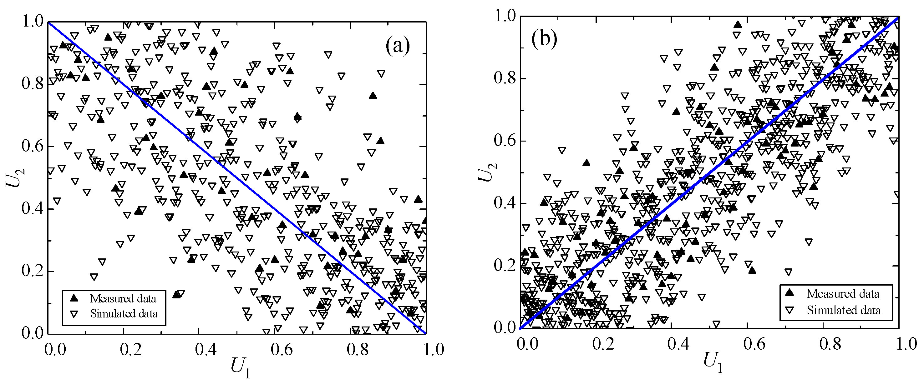
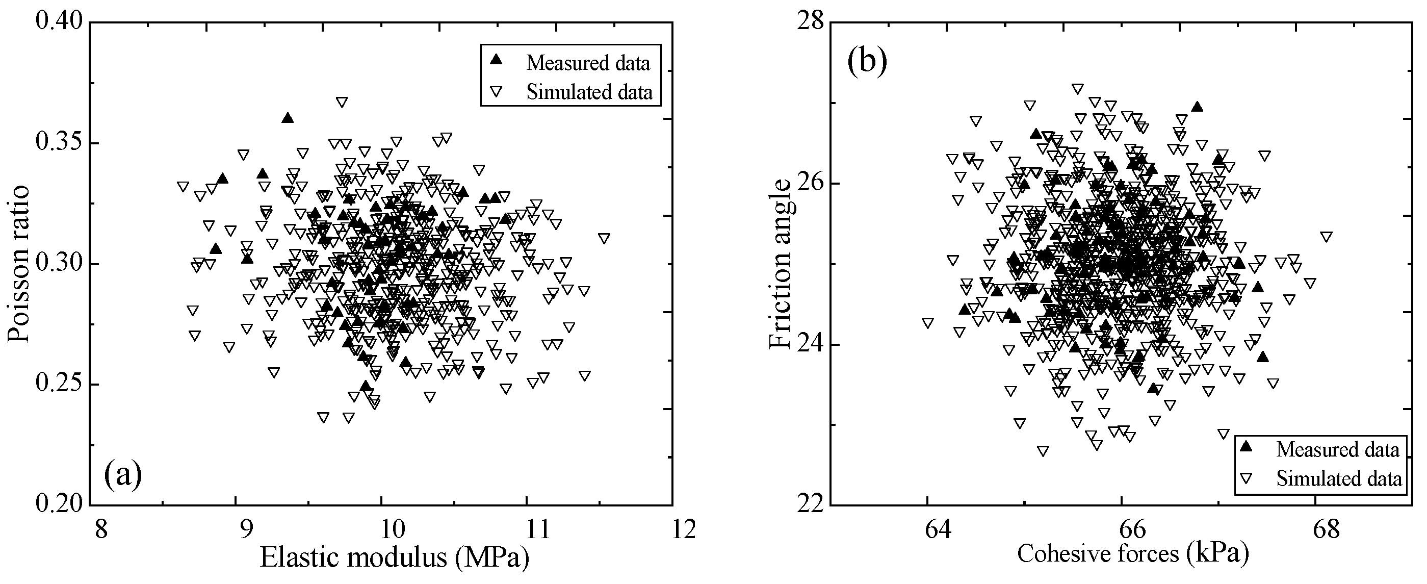
Copula theory provides a powerful framework for modeling complex dependence structures among soil parameters, overcoming the limitations of traditional correlation coefficients. The EM has a negative correlation with the PR, while the CF has a positively correlation with the FA. The discrete characteristics of the simulated data have similar discrete characteristics to those of the original data. The statistics of the simulated data and test data are basically the same. The bootstrap approach circumvents parametric assumptions by harnessing empirical data to improve the reliability in variable land subsidence analyses.

(3)

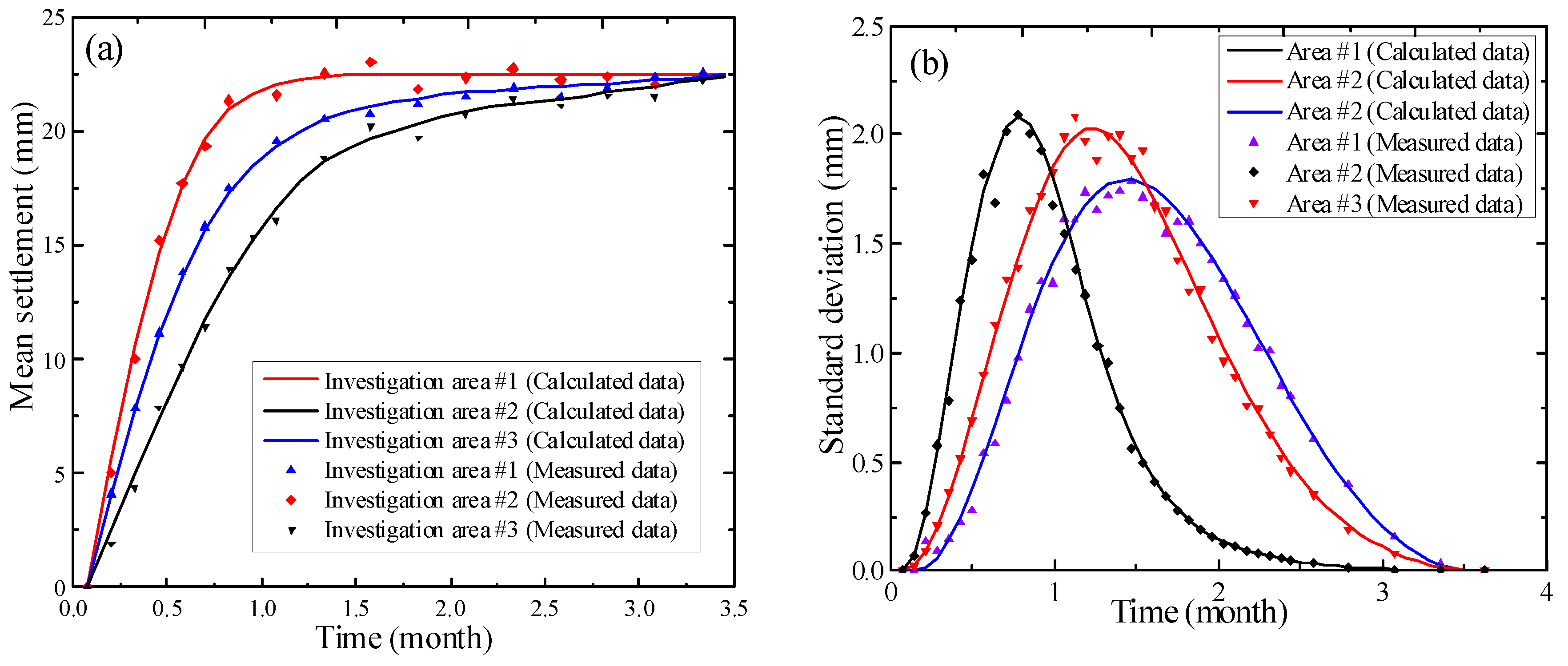
The test results of the mean settlement are basically the same as the simulation results. The stability analysis method for uncertain geotechnical properties for variable land subsidence processes in this paper is scientific and reasonable. The variable land subsidence follows a normal distribution with a significance level of 0.1. The influence of the variability parameter on the variable land subsidence processes is greater than that of the correlation structure.

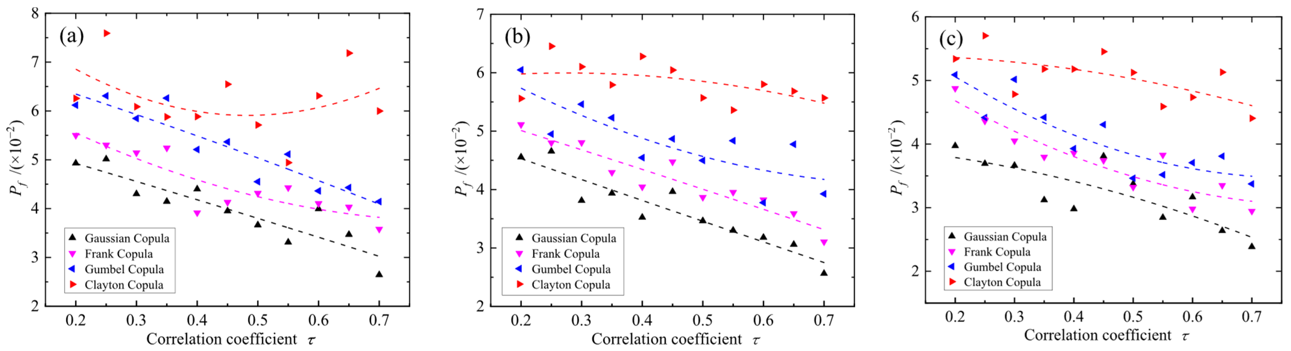
(4)

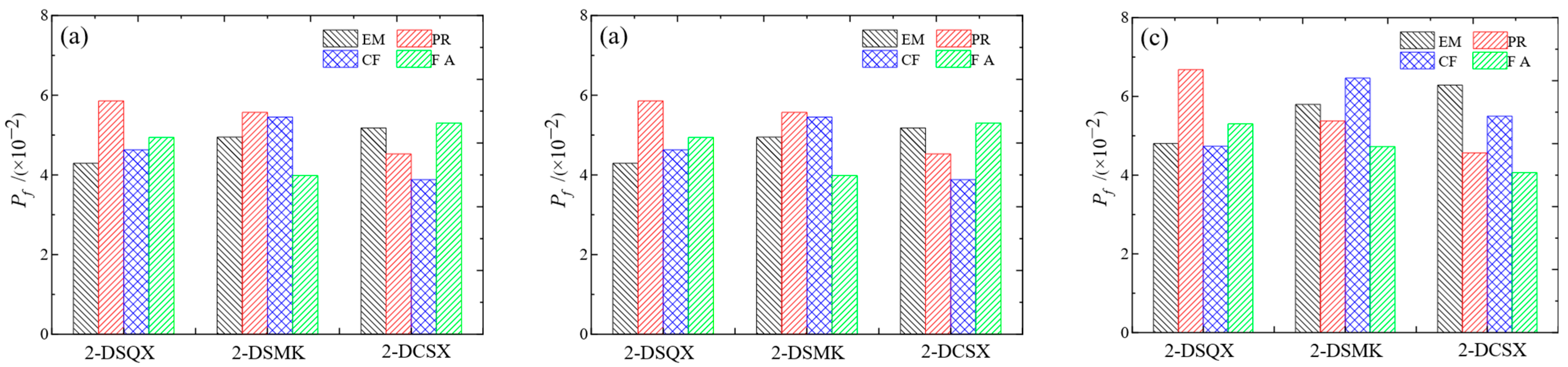
The failure probabilities of variable stratum settlement for different cross-correlations of geotechnical properties under copula conditions are different. When using the Clayton Copula to characterize the cross-correlation of the geotechnical properties, the failure probability is higher. When using the Gaussian Copula to characterize the cross-correlation of the geotechnical properties, the failure probability is smaller. It can be seen that different cross-correlation structures have different influences on the failure probability of variable stratum settlement.

The investigation of ground subsidence induced by uncertain soil properties presents a critical frontier in building engineering, demanding innovative approaches to address the spatiotemporal variability in soil behavior. Future research should prioritize integrating advanced in situ testing technologies and new materials [44], such as distributed fiber-optic sensing and real-time piezometric monitoring, to capture dynamic soil responses under variable loading conditions. Some limitations need to be further explained in this paper. The dual-yield surface model assumes coupled elastic–plastic behaviors, which may not fully represent the long-term viscoelastic effects observed in some clayey soils. However, this simplification enabled computationally efficient uncertainty quantification for preliminary risk assessment. The two-month monitoring period provided valuable insights but did not account for seasonal hydrological cycles or the extended consolidation processes typical of clayey strata. Future work will integrate multi-year monitoring data to enhance predictions of creep-induced settlement. Machine learning-enhanced numerical models could better quantify the uncertainties arising from heterogeneous lithologies, anisotropic permeability, and time-dependent consolidation processes, enabling probabilistic stability assessments. Additionally, the development of physics-informed surrogate models could bridge computational efficiency and accuracy for large-scale subsidence predictions. Interdisciplinary collaboration among geologists, hydrologists, and data scientists is essential to establish standardized protocols for characterizing site-specific subsidence mechanisms. Advances in this domain will enhance the predictive reliability for infrastructure resilience planning. This paradigm shift toward uncertainty-aware geotechnical systems will ultimately reduce the risks associated with land subsidence while optimizing resource allocation in building engineering.

References

1. El Shinawi, A.; Kuriqi, A.; Zelenakova, M.; Vranayova, Z.; Abd-Elaty, I. Land subsidence and environmental threats in coastal aquifers under sea level rise and over-pumping stress. J. Hydrol. 2022, 608, 127607. [Google Scholar] [CrossRef]
2. Ghorbani, Z.; Khosravi, A.; Maghsoudi, Y.; Mojtahedi, F.F.; Javadnia, E.; Nazari, A. Use of InSAR data for measuring land subsidence induced by groundwater withdrawal and climate change in Ardabil Plain, Iran. Sci. Rep. 2022, 12, 13998. [Google Scholar] [CrossRef]
3. Moradi, A.; Emadodin, S.; Beitollahi, A.; Abdolazimi, H.; Ghods, B. Assessments of land subsidence in Tehran metropolitan, Iran, using Sentinel-1A InSAR. Environ. Earth Sci. 2023, 82, 569. [Google Scholar] [CrossRef]
4. Wu, J.; Shi, B.; Gu, K.; Liu, S.; Wei, G. Evaluation of land subsidence potential by linking subsurface deformation to microstructure characteristics in Suzhou, China. Bull. Eng. Geol. Environ. 2021, 80, 2587–2600. [Google Scholar] [CrossRef]
5. Huang, Q.; Gou, Y.; Xue, L.; Yuan, Y.; Yang, B.; Peng, J. Model test study on the mechanical response of metro tunnel to land subsidence. Tunn. Undergr. Space Technol. 2023, 140, 105333. [Google Scholar] [CrossRef]
6. Gao, F.; Zhao, T.; Zhu, X.; Zheng, L.; Wang, W.; Zheng, X. Land subsidence characteristics and numerical analysis of the impact on major infrastructure in Ningbo, China. Sustainability 2022, 15, 543. [Google Scholar] [CrossRef]
7. Deng, S.; Yang, H.; Chen, X.; Wei, X. Probabilistic analysis of land subsidence due to pumping by Biot poroelasticity and random field theory. J. Eng. Appl. Sci. 2022, 69, 18. [Google Scholar] [CrossRef]
8. Intui, S.; Inazumi, S.; Soralump, S. Evaluation of land subsidence during groundwater recovery. Appl. Sci. 2022, 12, 7904. [Google Scholar] [CrossRef]
9. Khan, J.; Ren, X.; Hussain, M.A.; Jan, M.Q. Monitoring land subsidence using PS-InSAR technique in Rawalpindi and islamabad, Pakistan. Remote Sens. 2022, 14, 3722. [Google Scholar] [CrossRef]
10. Zevgolis, I.E.; Theocharis, A.I.; Koukouzas, N.C. Spatial Variability in Geotechnical Properties Within Heterogeneous Lignite Mine Spoils. Geosciences 2025, 15, 97. [Google Scholar] [CrossRef]
11. Nguyen, T.S.; Ngamcharoen, K.; Likitlersuang, S. Statistical characterisation of the geotechnical properties of Bangkok subsoil. Geotech. Geol. Eng. 2023, 41, 2043–2063. [Google Scholar] [CrossRef]
12. Nasir, A.; Butt, F.; Ahmad, F. Enhanced mechanical and axial resilience of recycled plastic aggregate concrete reinforced with silica fume and fibers. Innov. Infrastruct. Solut. 2025, 10, 1–17. [Google Scholar] [CrossRef]
13. Kalantari, A.R.; Johari, A.; Zandpour, M.; Kalantari, M. Effect of spatial variability of soil properties and geostatistical conditional simulation on reliability characteristics and critical slip surfaces of soil slopes. Transp. Geotech. 2023, 39, 100933. [Google Scholar] [CrossRef]
14. Zhao, T.; Wang, Y.; Xu, L. Efficient CPT locations for characterizing spatial variability of soil properties within a multilayer vertical cross-section using information entropy and Bayesian compressive sensing. Comput. Geotech. 2021, 137, 104260. [Google Scholar] [CrossRef]
15. Alamanis, N.; Dakoulas, P. Effects of spatial variability of soil properties and ground motion characteristics on permanent displacements of slopes. Soil Dyn. Earthq. Eng. 2022, 161, 107386. [Google Scholar] [CrossRef]
16. Ghaaowd, I.; Faisal, A.H.M.H.; Rahman, M.H.; Abu-Farsakh, M. Evaluation of site variability effect on the geotechnical data and its application. Geotech. Test. J. 2021, 44, 971–985. [Google Scholar] [CrossRef]
17. Guan, Z.; Wang, Y.; Phoon, K.K. Dictionary learning of spatial variability at a specific site using data from other sites. J. Geotech. Geoenviron. Eng. 2024, 150, 04024072. [Google Scholar] [CrossRef]
18. Li, X.; Zhang, Y.; Li, Z.; Yang, Z.; Qi, X. A coupled probabilistic site characterization method for estimating soil stratification and spatial variability using multiple-source site investigation data. Eng. Geol. 2025, 351, 108024. [Google Scholar] [CrossRef]
19. Ma, G.; Rezania, M.; Nezhad, M.M. Stochastic assessment of landslide influence zone by material point method and generalized geotechnical random field theory. Int. J. Geomech. 2022, 22, 04022002. [Google Scholar] [CrossRef]
20. Yoshida, I.; Tomizawa, Y.; Otake, Y. Estimation of trend and random components of conditional random field using Gaussian process regression. Comput. Geotech. 2021, 136, 104179. [Google Scholar] [CrossRef]
21. Rawat, S.; Saliba, P.; Estephan, P.C.; Ahmad, F.; Zhang, Y. Mechanical performance of Hybrid Fibre Reinforced Magnesium Oxychloride Cement-based composites at ambient and elevated temperature. Buildings 2024, 14, 270. [Google Scholar] [CrossRef]
22. Phoon, K.K.; Ching, J.; Shuku, T. Challenges in data-driven site characterization. Georisk Assess. Manag. Risk Eng. Syst. Geohazards 2022, 16, 114–126. [Google Scholar] [CrossRef]
23. Wang, C.; Wang, K.; Tang, D.; Hu, B.; Kelata, Y. Spatial random fields-based Bayesian method for calibrating geotechnical parameters with ground surface settlements induced by shield tunneling. Acta Geotech. 2022, 17, 1503–1519. [Google Scholar] [CrossRef]
24. Choudhuri, K.; Chakraborty, D. Probabilistic analyses of three-dimensional circular footing resting on two-layer c–ϕ soil system considering soil spatial variability. Acta Geotech. 2022, 17, 5739–5758. [Google Scholar] [CrossRef]
25. Ahmad, F.; Rawat, S.; Yang, R.C.; Zhang, L.; Zhang, Y.X. Fire resistance and thermal performance of hybrid fibre-reinforced magnesium oxychloride cement-based composites. Constr. Build. Mater. 2025, 472, 140867. [Google Scholar] [CrossRef]
26. Gong, W.; Zhao, C.; Juang, C.H.; Zhang, Y.; Tang, H.; Lu, Y. Coupled characterization of stratigraphic and geo-properties uncertainties–a conditional random field approach. Eng. Geol. 2021, 294, 106348. [Google Scholar] [CrossRef]
27. Di, H.; Zhou, S.; Yao, X.; Tian, Z. In situ grouting tests for differential settlement treatment of a cut-and-cover metro tunnel in soft soils. Bull. Eng. Geol. Environ. 2021, 80, 6415–6427. [Google Scholar] [CrossRef]
28. Wang, Y.; Zhang, F.; Liu, F.; Wang, X. Full-scale in situ experimental study on the bearing capacity of energy piles under varying temperature and multiple mechanical load levels. Acta Geotech. 2024, 19, 401–415. [Google Scholar] [CrossRef]
29. Zhang, P.; Jin, Y.F.; Yin, Z.Y. Machine learning—Based uncertainty modelling of mechanical properties of soft clays relating to time-dependent behavior and its application. Int. J. Numer. Anal. Methods Geomech. 2021, 45, 1588–1602. [Google Scholar] [CrossRef]
30. Wang, Z.Z.; Xiao, C.; Goh, S.H.; Deng, M.X. Metamodel-based reliability analysis in spatially variable soils using convolutional neural networks. J. Geotech. Geoenviron. Eng. 2021, 147, 04021003. [Google Scholar] [CrossRef]
31. Shi, C.; Wang, Y. Assessment of reclamation-induced consolidation settlement considering stratigraphic uncertainty and spatial variability of soil properties. Can. Geotech. J. 2022, 59, 1215–1230. [Google Scholar] [CrossRef]
32. Alibeikloo, M.; Khabbaz, H.; Fatahi, B. Random field reliability analysis for time-dependent behaviour of soft soils considering spatial variability of elastic visco-plastic parameters. Reliab. Eng. Syst. Saf. 2022, 219, 108254. [Google Scholar] [CrossRef]
33. Yang, Z.; Chen, J.; Feng, Y.; Li, X. Probabilistic analysis of offshore single pile composite foundation considering rotated anisotropy spatial variability of multi-layered soils. Comput. Geotech. 2025, 182, 107159. [Google Scholar] [CrossRef]
34. Hu, Y.; Wang, Y.; Phoon, K.K.; Beer, M. Similarity quantification of soil spatial variability between two cross-sections using auto-correlation functions. Eng. Geol. 2024, 331, 107445. [Google Scholar] [CrossRef]
35. Bao, X.; Li, J.; Shen, J.; Chen, X.; Zhang, C.; Cui, H. Comprehensive multivariate joint distribution model for marine soft soil based on the vine copula. Comput. Geotech. 2025, 177, 106814. [Google Scholar] [CrossRef]
36. Cao, J.; Wang, T.; Sheng, M.; Huang, Y.; Zhou, G. A Copula method for modeling the intensity characteristic of geotechnical strata of roof based on small sample test data. Geomech. Eng. 2024, 36, 601–618. [Google Scholar]
37. Zhou, X.; Lu, D.; Zhang, Y.; Du, X.; Rabczuk, T. An open-source unconstrained stress updating algorithm for the modified Cam-clay model. Comput. Methods Appl. Mech. Eng. 2022, 390, 114356. [Google Scholar] [CrossRef]
38. Li, Z.; Zhao, G.F.; Wei, X.; Deng, X. Numerical modelling of multiple excavations in an ultra-deep foundation using an enhanced distinct lattice spring model with modified cam clay model. Tunn. Undergr. Space Technol. 2024, 152, 105875. [Google Scholar] [CrossRef]
39. Chi, S.; Feng, W.; Jia, Y.; Zhang, Z. Stochastic finite-element analysis of earth–rockfill dams considering the spatial variability of soil parameters. Int. J. Geomech. 2022, 22, 04022224. [Google Scholar] [CrossRef]
40. Chen, X.J.; Fu, Y.; Liu, Y. Random finite element analysis on uplift bearing capacity and failure mechanisms of square plate anchors in spatially variable clay. Eng. Geol. 2022, 304, 106677. [Google Scholar] [CrossRef]
41. Ebner, B.; Liebenberg, S.C.; Visagie, I.J.H. A new omnibus test of fit based on a characterization of the uniform distribution. Statistics 2022, 56, 1364–1384. [Google Scholar] [CrossRef]
42. Raza, M.U.; Butt, F.; Ahmad, F.; Waqas, R.M. Seismic safety assessment of buildings and perceptions of earthquake risk among communities in Mingora, Swat, Pakistan. Innov. Infrastruct. Solut. 2025, 10, 1–18. [Google Scholar] [CrossRef]
43. Zhang, W.; Huang, Z.; Zhang, J.; Zhang, R.; Ma, S. Multifactor uncertainty analysis of construction risk for deep foundation pits. Appl. Sci. 2022, 12, 8122. [Google Scholar] [CrossRef]
44. Ahmad, F.; Rawat, S.; Zhang, L.; Fanna, D.J.; Soe, K.; Zhang, Y.X. Effect of Metakaolin and Ground Granulated Blast Furnace Slag on the Performance of Hybrid Fibre-Reinforced Magnesium Oxychloride Cement-Based Composites. Int. J. Civ. Eng. 2025, 23, 853–868. [Google Scholar] [CrossRef]
Figure 1. Measured soil properties of building foundations at different locations in the investigation areas: (a) EM; (b) PR; (c) CF; (d) FA.
Buildings 15 02369 g001
Figure 2. Statistical distribution of measured soil properties of building foundations in the investigation areas: (a) EM; (b) PR; (c) CF; (d) FA.
Buildings 15 02369 g002
Figure 3. Fitted curves of the fluctuation scale of the random field in different directions. (a) Vertical direction of the stratum; (b) horizontal direction of the stratum.
Buildings 15 02369 g003
Figure 4. Autocorrelation function structures of spatial variability characterization for uncertain soil properties of building foundations: (a) EM; (b) PR; (c) CF; (d) FA.
Buildings 15 02369 g004
Figure 5. Discrete uniformly distributed variables of cross-correlation characterization for uncertain soil properties of building foundations: (a) EM and PR; (b) CF and FA.
Buildings 15 02369 g005
Figure 6. Discrete correlation distribution variables of cross-correlation characterization for uncertain soil properties of building foundations: (a) EM and PR; (b) CF and FA.
Buildings 15 02369 g006
Figure 7. Statistical characteristics of simulated soil properties of building foundation in the investigation area. (a) COV. (b) SOF. (c) ACD.
Buildings 15 02369 g007
Figure 8. Comparison of measurement results and calculation results for the settlement properties of building foundation soils.
Buildings 15 02369 g008
Figure 9. Failure probabilities of variable settlement properties of building foundations for different spatial variations of soil properties: (a) investigation area #1; (b) investigation area #2; (c) investigation area #3.
Buildings 15 02369 g009
Figure 10. Failure probabilities of variable settlement properties of building foundations for different cross-correlation variations under positive copula conditions: (a) investigation area #1; (b) investigation area #2; (c) investigation area #3.
Buildings 15 02369 g010
Figure 11. Failure probabilities of variable settlement properties of building foundations for different cross-correlation variations under negative copula conditions: (a) investigation area #1; (b) investigation area #2; (c) investigation area #3.
Buildings 15 02369 g011