Abstract
The dissimilar steel welded joint is divided into three pieces, parent material–weld metal–parent material, by the integrity identification of BS7910-2013. In reality, the undermatched welded joint geometry is different: parent material–heat affected zone (HAZ)–fusion line–weld metal. A combination of the CF62 (parent material) and E316L (welding rod) was the example undermatched welded joint, whose geometry was divided into four pieces to investigate the fracture toughness of the joint by experiments and the extended finite element method (XFEM) calculation. The experimental results were used to change the fracture toughness of the undermatched welded joint, and the XFEM results were used to amend the fracture toughness calculation method with a new definition of the crack length. The research results show that the amendment of the undermatched welded joint geometry expresses more accuracy of the fracture toughness of the joint. The XFEM models were verified as valid by the experiment. The amendment of the fracture toughness calculation method expresses a better fit by the new definition of the crack length, in accordance with the crack route simulated by the XFEM. The results after the amendment coincide with the reality in engineering.
1. Introduction
1.1. The Undermatched Welded Joint
High-strength low-alloy (HSLA) steel is commonly used for petrochemical equipment. The development of special electrodes for the new HSLA is expensive and time-consuming. Ready-made lower strength electrodes for HSLA are a good choice to fabricate the undermatched welded joint. The undermatched welded joint has a low crack tendency and is economical within a wide range of matching ratios [1].
1.2. The Integrity Identification of the Undermatched Welded Joint
The integrity identification of BS7910-2013 [2] shows the three pieces of the undermatched welded joint, parent material–weld metal–parent material, which is like a sandwich structure. In reality, the undermatched welded joint geometry is different [3], parent material–heat affected zone (HAZ)–fusion line–weld metal, as Figure 1a shows. Figure 1b shows the different grain sizes of the different areas of the undermatched welded joint. The blue line in the figure is the line between the HAZ and the parent material. The combination of CF62 (parent material) and E316L (welding rod) is the example undermatched welded joint in this study. The fracture toughness of the different areas was researched by experiments and extended finite element method (XFEM) simulations in this paper. The XFEM models of the different areas of the undermatched welded joint were built and verified as valid by the experiments.
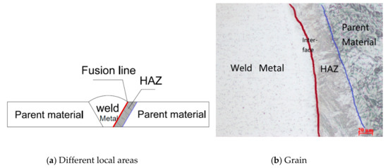
Figure 1.
Different areas of the investigated welded joint. (a) Different local areas; (b) Grain.
1.3. The Research Status of XFEM
The extended finite element method (XFEM) was put forward by Belytschko [4], an American professor, and was used to research the crack growth route. Compared to the traditional finite element, the XFEM simulated the crack initiation and growth without the need to refresh the meshing, reducing the workload. Sukumar et al. [5] promoted the 2D XFEM crack model to a 3D XFEM crack model. Legay [6] and Ventura et al. [7] researched the blending element (shown in Figure 2) to improve the convergence and precision of the simulation. Menouillard [8] improved integral stability. Zhuang and Cheng [9] realized the fusion line crack extension between the dissimilar steels by the XFEM.
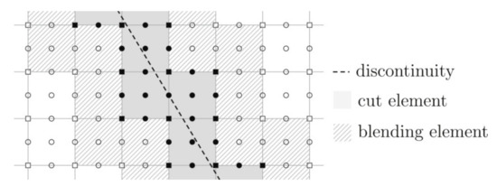
Figure 2.
Planar crack, cut element, and blending element.
Research of the XFEM began late in China. Xiujun Fang of Tsinghua University researched the cohesive crack model based on the XFEM in 2007 [10]. Hai Xie of Shanghai Jiaotong University developed the XFEM with the ABAQUS User Subroutine in 2009 [11]. Yehai Li of Nanjing University of Aeronautics and Astronautics researched the interfacial crack growth of the dissimilar material in 2012 [12]. Shaoyun Zhang of Zhejiang University researched the helical crack growth by the XFEM in 2013 [13]. Zhifeng Yang of Nanjing Tech University developed the 2D elastic-plastic crack XFEM model and verified its validity by the J integral in 2014 [14]. Yixiu Shu of the Northwestern Polytechnical University analyzed the multiple crack interaction problems by the XFEM in 2015 [15]. Yang Zhang of Harbin Engineering University applied a 3D crack to the pressure vessel by the XFEM in 2015 [16]. Zhen Wang and Tiantang Yu researched the adaptive multiscale XFEM model for 3D crack problems in 2016 [17].
1.4. The Welding of the Undermatched Joint
The size of the weld plate is 600 × 400 × 40 mm (length, width, and thickness, respectively) with an X-shaped groove, shown in Figure 3. The welding rod (E316L) is the special electrode for 316L stainless steel. The welding parameters are listed in Table 1, in accordance with the criteria of ASME-VIII [18]. Table 2 and Table 3 list the chemical composition tested results of CF62 and E316L. Table 4 and Table 5 list the mechanical properties of the CF62 steel and the E316L steel, respectively.
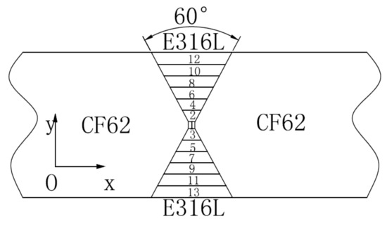
Figure 3.
The investigated welded joint.

Table 1.
Welding parameters of the undermatched welded joint adapted from [18], with permission from American Society of Mechanical Engineers, 2019.
Table 2.
Chemical composition of CF62 (wt.%).
Table 3.
Chemical composition of E316L(wt.%).
Table 4.
Mechanical properties of CF62 reproduced from [19], with permission from Taiyuan University of Science and Technology, 2019.
Table 5.
Mechanical properties of E316L reproduced from [20], with permission from welding technology, 2019.
1.5. The Fracture Toughness Calculation Method
ASTM 1820-18 [21] is the newest standard test method for the measurement of fracture toughness. Fracture toughness is calculated by the relationship between the J integral and the crack length, [21]:
where:
- is the area under force versus displacement, as shown in Figure 4;
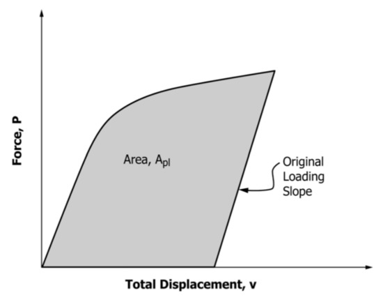 Figure 4. Definition of the area for the J calculation using the basic method.
 - is either 1.9 if the load-line displacement is used for or 3.667 − 2.199() + 0.437 if the recorded crack mouth opening displacement is used for ;
- is the net specimen thickness;
- is W − .
The crack length, , is calculated by the displaced force point with Equation (3):
where:
where:
- is the measured specimen elastic compliance () (at the load-line);
- is the initial half-span of the load points (center of the pin holes);
- D is one-half of the initial distance between the displacement measurement points;
- is the radius of the rotation of the crack center line, (W+a)/2, where a is the updated crack size.
Figure 5a shows the relationship between the crack rotation angle, , and the respective crack length, [21]. The crack rotation angle, , is calculated by Equation (7). Figure 5a shows that the crack length, , was equal to the length parallel to the center line of the compact tension (CT) samples. The crack deflection has not been considered in the crack length calculation in the criteria.
where is the total measured load-line displacement at the beginning of the i-th unloading/reloading cycle.
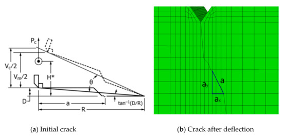
Figure 5.
Crack rotation angle, , of the compact tension (CT) specimens. (a) Initial crack; (b) Crack after deflection.
Figure 5b shows the crack route after the crack deflection. It shows the crack length after the deflection, . The crack length in the criteria of ASTM 1820-18 is = , which means that . Therefore, the crack length, , calculated by the criteria of ASTM 1820-18, was smaller than the true crack length after the deflection, . The fracture toughness calculation method was then amended by the crack length after the deflection was simulated by the XFEM.
The division of the geometry (parent material–HAZ–fusion line–weld metal) of the undermatched welded joint and the experimental results changed the fracture toughness of the dissimilar steel welded joint. The crack length amendment after the deflection defined a new fracture toughness calculation method of the dissimilar welded joint.
1.6. J Integral and the Fracture Toughness Value,
The J integral was put forward by Rice [22]. Figure 6a shows the integral loop/area around the crack tip. Equation (8) is calculated with the equivalent integral region to deal with the stress and the strain of Figure 6b [22]. Figure 6c shows the integral area, which contains a heterogeneous material interface. In [23], it was verified that the interface integral area when the crack tip is under a constant temperature with a pure mechanical load. Equation (8) is applicable to calculate the J integral for the investigated welded joint in this paper.
where is the component of the displacement vector; is the tiny increment area on the integral path, ; is the strain energy density factor; and q(x,y) is a mathematical function, which is q = 0 in the outer boundary and q = 1 in the other places of the regional; and , are listed in Equation (9).
where is the stress tensor and is the strain tensor.
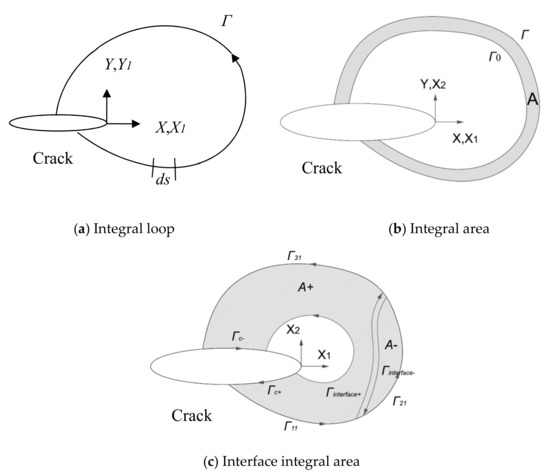
Figure 6.
Counterclockwise integral loop around the crack tip. (a) Integral loop; (b) Integral area; (c) Interface integral area.
BS7910-2013 [2] gives Equation (10), which shows the relationship between the value and the fracture toughness value, , during the elastic stage:
where is the elastic modulus and is the Poisson’s ratio.
2. Experiments
2.1. The Fracture Toughness Experiments
The fracture toughness of the different areas of the joint geometry (parent material–HAZ–fusion line–weld metal) was tested with the individual CT specimens that were taken from the undermatched welded joint. The crack initiated and grew along the center line of the CT specimens during the experiments. The center lines in the different areas of the joint present the locations of the CT specimens in the dissimilar joint, as seen in Figure 7. The CT size is shown in Figure 8.
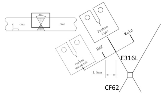
Figure 7.
Center lines of the CT specimens in the investigated welded joint.
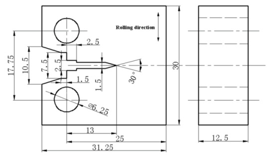
Figure 8.
Size of the CT specimens.
The fracture toughness was tested with the MTS-809 (MTS Systems Cor., Eden Prairie, MN, USA). The local fracture surfaces taken by SEM of the different areas of the joint geometry are shown in Figure 9. Figure 9b shows that the crack initiated from the high-strength region (parent material) and deflected to the lower strength region (weld metal) in the HAZ. Figure 10 depicts the HAZ fracture surface macro-image, which indicates the parent material (PM) region and the weld metal region. It means that the crack deflection existed in the dissimilar material during the experiment. The experimental process was in accordance with the criteria of ASTM 1820-18 [21], and the results of the J integral and the crack length, Δa, were managed under the regulations.
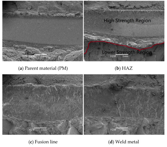
Figure 9.
Fracture surfaces after the fracture toughness experiment. (a) Parent material (PM); (b) HAZ; (c) Fusion line; (d) Weld metal.
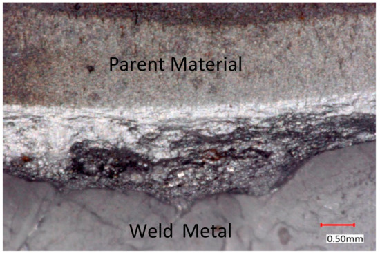
Figure 10.
HAZ fracture surface macro-image.
2.2. The Tensile Experiments
The maximum stress damage of the parent material and the weld metal was needed to build the XFEM models. It was tested with a flat tensile specimen, which was 0.8 mm in thickness. Figure 11a shows the location of the tensile specimen, which was taken from the parent material to the weld metal and is parallel to the fusion line. Figure 11b shows the shape and dimensions of the flat tensile specimen.
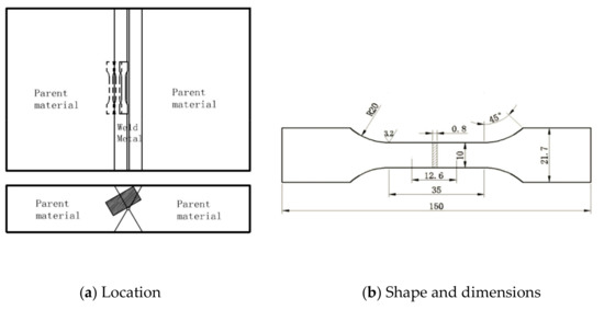
Figure 11.
The location and size of the flat tensile specimen. (a) Location; (b) Shape and dimensions.
3. XFEM Models
A pre-crack was needed when the 1/2 CT specimen was tested and the pre-crack length was 1.5 mm, in accordance with the criteria of the ASTM 1820-18 regulation. The XFEM models were built with a 1.5 mm pre-crack.
The four XFEM models were the parent material, weld metal, fusion line (a combination of PM and weld metal), and HAZ. The mechanical properties were tested by the flat tensile specimen. There were two important parameters—the maximum stress damage, −, and the equivalent energy release rate, . In [14,24], the relationship between, , and the tensile strength, . When the maximum energy release rate (MERR), , is equal to the threshold, , the crack begins to initiate. The MERR, , is calculated in Equation (11), and the threshold is calculated in Equation (12) [13]:
where is the elastic modulus, is the Poisson’s ratio, is the applied tensile stress intensity factor of Mode , and is the applied tensile stress intensity factor of Mode .
There are three kinds of crack mode—the opening crack mode (Mode ), the sliding crack mode (Mode ), and the tearing crack mode (Mode III). The experimental and XFEM simulation load is perpendicular to the crack surface. The research crack in this paper is the opening crack mode(Mode ). The MERR threshold, , is related to the critical stress intensity factor of Mode , which is :
Since the crack mode in this paper is Mode , [13]. The XFEM simulation properties of CF62 and E316L are listed in Table 6.
Table 6.
Mechanical properties of the crack propagation.
Figure 12 shows the meshing of the XFEM of the 1/2CT. The sparse meshing elements in the XFEM are applicable [25,26,27]. Figure 13 shows the dissimilar material XFEM models of the joint geometry with the material printed on their parts. The parent material and weld metal XFEM models are not shown since they are the uniform material model, i.e., they are the material printed on the whole model.
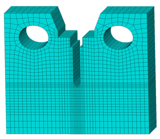
Figure 12.
The meshing model of the extended finite element method(XFEM).
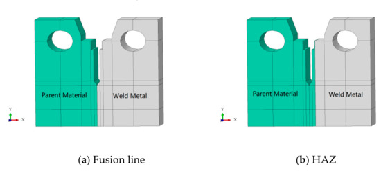
Figure 13.
The dissimilar material XFEM models. (a) Fusion line; (b) HAZ.
4. The Fracture Toughness of the Undermatched Welded Joint
4.1. Fracture Toughness of the Undermatched Welded Joint
The test results of the J integral and crack length, , are fitted by Equation (13) in the criteria of ASTM 1820-18 [21]:
The experimental data and the resistance equations of the different areas of the joint geometry are listed in Table 7 and Table 8, respectively. The resistance curves are shown in Figure 14.
Table 7.
Experimental data.
Table 8.
The resistance equations and the value of the undermatched welded joint.
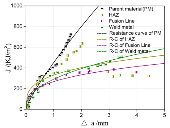
Figure 14.
The ensemble of the J-∆a resistance curves of the undermatched welded joint.
4.2. Amendment of HAZ Fracture Toughness
Figure 15a shows the fracture surface of the HAZ and shows that there was a 1.04 mm length of the smooth fracture surface and a 1.07 mm length of the parent material fracture surface. The fusion line between the parent material and the weld metal is marked with a red line. The weld metal fracture surface is below the red line.
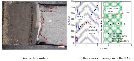
Figure 15.
Fracture toughness results of the HAZ. (a) Fracture surface; (b) Resistance curve regions of the HAZ.
Figure 15b shows the resistance curve regions of the HAZ. It shows that in the initial crack ) the R-curve fits the resulting data points well. The parent material region is next to the fitting region: . The J integral is larger than the curve point which shows the parent material’s fracture toughness. After the crack grew across to the weld metal region, the J integral was smaller than the R-curve points.
Haitao Wang tested and simulated the crack growth paths in a dissimilar metal welded joint and found that the crack deflected to the soft area during the experiment [28,29]. Longchao Cao [30] and Pavel Podany [31] researched the microstructure and the local mechanical properties of the dissimilar butt joints. Jianbo Li [32] studied the fracture toughness near the fusion line (HAZ and fusion line) of the dissimilar material and, in addition, found the crack deflection. The HAZ experimental results demonstrated the crack deflection when the CT specimens were tested. The resistance curve of the HAZ (Figure 15b) shows that the fracture toughness of the undermatched welded joint needs to be amended. The crack deflection shows that the crack length test method needs to be amended as well.
As there was a misfit of the data points in the two regions and the lower strength region was the weld metal region, which was below the high-strength region, the HAZ was considered to be the high-strength region. The crack initiated in the HAZ high-strength region and then deflected to the weld metal region. During the crack growth process, the crack crossed the fusion line between the high-strength region and the weld metal region. Figure 9b shows the local fracture surface figure taken by SEM, which shows the location of the high-strength region and the weld metal region (lower strength region).
Table 9 lists the resistance equations after the amendment of the different areas (parent material–HAZ–fusion line–weld metal) of the undermatched welded joint geometry. The fusion line crack deflection initiated in the pre-crack stage and the crack growth of the fusion line (the heterogeneous material XFEM model) were always in the weld metal region.
Table 9.
The resistance equations and the values of the undermatched welded joint after amending.
Figure 16 shows the resistance curves of the high-strength regions of the HAZ after amending. The figure shows that the HAZ is more applicable between the resistance curve and the data points after amending.
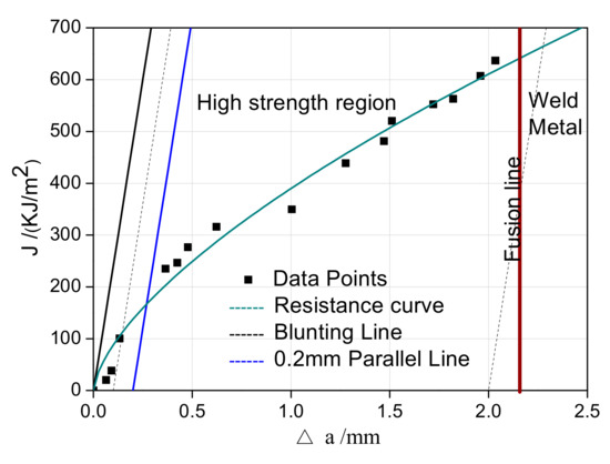
Figure 16.
Resistance curves of the HAZ after amending.
4.3. J Integral Verification of XFEM
The XFEM gives the J integral of the crack growth, which is used to compare the experimental J-Δa resistance curves. The XFEM models of the parent material and the weld metal were verified, respectively, by the experimental results. Figure 17 and Figure 18 are the XFEM results of the parent material and the weld metal. Figure 17a and Figure 18a show the CT stress distribution, and Figure 17b and Figure 18b show the crack route.
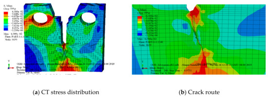
Figure 17.
XFEM result of the parent material. (a) CT stress distribution; (b) Crack route.
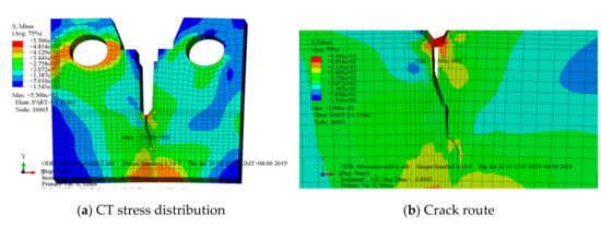
Figure 18.
XFEM result of the weld metal. (a) CT stress distribution; (b) Crack route.
There are five J integral routes when the XFEM model outputs the J integral and the results are the same. The J integral result is independent of the route, which has been demonstrated previously [27,33,34].
Figure 19 shows the comparison of the experimental J-Δa resistance curves and the J integral data point output of the XFEM. The figure shows that the data point output of the XFEM coincides well with the experimental J-Δa resistance curves. This means that the XFEM models in this paper are valid for the undermatched welded joint.
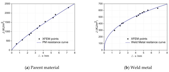
Figure 19.
J integral verification of the XFEM. (a) Parent material; (b) Weld metal.
5. Amendment of the Fracture Toughness Calculation Method
Table 10 lists the resistance equations of the investigated welded joint after the crack length amendment. Figure 20 shows the homogeneous material XFEM models’ (PM and weld metal) resistance curves after amendment, while Figure 21 shows the heterogeneous material XFEM models’ (fusion line and HAZ) resistance curves after amendment. Figure 21a shows the resistance curve of the fusion line, and Figure 21b shows that of the HAZ high-strength region.
Table 10.
The resistance equations and the and values of the undermatched welded joint after the crack amendment based on the XFEM.
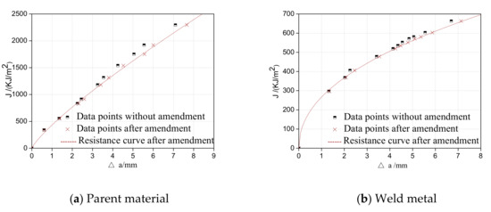
Figure 20.
Resistance curves after the crack length amendment of the homogeneous material. (a) Parent material; (b) Weld metal.
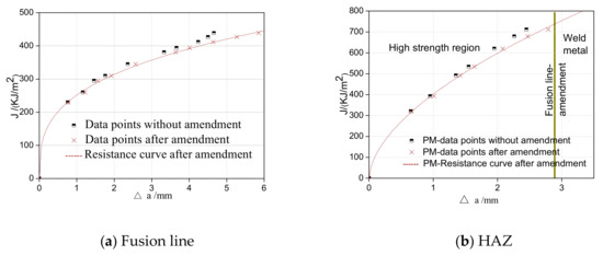
Figure 21.
Resistance curves after the crack length amendment of the heterogeneous material. (a) Fusion line; (b) HAZ.
The crack length amendment results show that the fracture toughness calculation method of the undermatched welded joint needed to be amended, due to the crack growth deflection of the heterogeneous material.
The fracture toughness of the investigated welded joint was given by experimenting with the different areas of the joint (parent material–fusion line–HAZ–weld metal). In addition, the fracture toughness calculation method was amended based on the XFEM models of the heterogeneous material in this paper.
6. Conclusions
The division of the dissimilar steel welded joint geometry of the current integrity identification needed to be amended to four pieces: parent material–HAZ–fusion line–weld metal. In accordance with this new division of the undermatched welded joint, XFEM models of the undermatched welded joint were built to calculate their fracture toughness. The conclusions are as follows:
- (1)
- The different areas (parent material–HAZ–fusion line–weld metal) of the undermatched welded joint geometry were tested to obtain the fracture toughness of the investigated welded joint. During the experiments, the fracture toughness of the joint changed in accordance with the crack deflection.
- (2)
- In this study, XFEM models of the homogeneous material and the heterogeneous material, i.e., the different areas of the undermatched welded joint geometry, were built to calculate the crack route.
- (3)
- The experimental results of the J-Δa resistance curve were compared to the XFEM calculation results to verify the validity of the XFEM to the undermatched welded joint.
- (4)
- The crack length amendment was in accordance with the XFEM simulation result—the crack route. The fracture toughness calculation method was amended by the crack length amendment after the deflection of the heterogeneous material by the XFEM.
Author Contributions
Y.Q. is mainly on the Methodology, Software, Validation, Formal Analysis, Investigation, Data Curation, Writing-Original Draft Preparation, Writing-Review & Editing. J.Z. is mainly on Writing-Review & Editing, Visualization, Supervision, Funding Acquisition.
Funding
This research was funded by the National Key Research and Development Program of China [2016YFC0801905].
Conflicts of Interest
The authors declare no conflict of interest.
References
- Wen, X.; Wang, P.; Dong, Z.B.; Liu, Y.; Fang, H.Y. Nominal stress-based equal-fatigue bearing-capacity design of under-matched HSLA steel butt-welded joints. Metals 2018, 8, 880. [Google Scholar] [CrossRef]
- BS7910:2013+A1:2015, Guide to Methods for Assessing the Acceptability of Flaws in Metallic Structures; BSI Standards Limited: London, UK, 2015.
- Baris Basyigit, A.; Murat, M.G. The Effects of TIG Welding Rod Compositions on Microstructural and Mechanical Properties of Dissimilar AISI 304L and 420 Stainless Steel Welds. Metals 2018, 8, 972. [Google Scholar] [CrossRef]
- Belytschko, T.; Black, T. Elastic crack growth in finite elements with minimal remeshing. Int. J. Numer. Methods Eng. 1999, 45, 601–620. [Google Scholar] [CrossRef]
- Sukumar, N.; Moes, N.; Moran, B.; Belytschko, T. Extended finite element method for three-dimensional crack modeling. Int. J. Numer. Methods Eng. 2000, 48, 1549–1570. [Google Scholar] [CrossRef]
- Legay, A.; Wang, H.W.; Belytschko, T. Strong and weak arbitrary discontinuities in spectral finite elements. Int. J. Numer. Methods Eng. 2005, 64, 991–1008. [Google Scholar] [CrossRef]
- Ventura, G.; Moran, B.; Belytschko, T. Dislocations by partition of unity. Int. J. Numer. Methods Eng. 2005, 62, 1463–1487. [Google Scholar] [CrossRef]
- Menouillard, T.; Rethore, J.; Combescure, A.; Bung, H. Efficient explicit time stepping for the extended finite element method (XFEM). Int. J. Numer. Methods Eng. 2006, 68, 911–939. [Google Scholar] [CrossRef]
- Zhuang, Z.; Cheng, B.B. Equilibrium state of mode-I sub-interfacial crack growth in bi-materials. Int. J. Fract. 2011, 170, 27–36. [Google Scholar] [CrossRef]
- Fang, X.J.; Jin, F.; Wang, J.T. Cohesive crack model based on extended finite element method. J. Tsinghua Univ. Sci. Tech. 2007, 47, 344–347. (In Chinese) [Google Scholar]
- Xie, H.; Feng, M.L. Implementation of Extended Finite Element Method with ABAQUS User Subroutine. J. Shanghai Jiaotong Univ. 2009, 43, 1644–1648. (In Chinese) [Google Scholar]
- Li, Y. Research on Interfacial Crack Propagation Using ABAQUS: Application to Artificial Ice Shape. Ph.D. Thesis, Nanjing University of Aeronautics and Astronautics, Nanjing, China, 2012. (In Chinese). [Google Scholar]
- Zhang, S. Study on Helical Crack Propagation by Extended Finite Element Method. Ph.D. Thesis, Zhejiang University, Hangzhou, China, 2013. (In Chinese). [Google Scholar]
- Yang, Z.; Zhou, C.; Dai, Q. Elastic-plastic crack propagation based on extended finite element method. J. Nanjing Tech Univ. (Nat. Sci. Ed.) 2014, 36, 50–57. (In Chinese) [Google Scholar]
- Shu, Y.X.; Li, Y.Z.; Jiang, W.; Jia, Y.X. Analyzing Multiple Crack Propagation Using Extended Finite Element Method(X-FEM). J. Northwest. Polytech. Univ. 2015, 33, 197–203. (In Chinese) [Google Scholar]
- Zhang, Y. Application Research of the Extended Finite Element Method on the Cracks in Pressure Vessel. Ph.D. Thesis, Harbin Engineering University, Harbin, China, 2015. (In Chinese). [Google Scholar]
- Wang, Z.; Yu, T.T. Adaptive multiscale extended finite element method for modeling three-dimensional crack problems. Eng. Mech. 2016, 33, 32–38. (In Chinese) [Google Scholar]
- ASME. ASME Boiler & Pressure Vessel Code, Section VIII, Division 1; American Society of Mechanical Engineers: New York, NY, USA, 2010. [Google Scholar]
- Gan, H. Effect of Cold Treatment Temperature on Microstructure and Mechanical Properties of Forged Low Alloy High Strength Steel. Ph.D. Thesis, Taiyuan University of Science and Technology, Taiyuan, China, 2012. (In Chinese). [Google Scholar]
- Zhu, P.; Chen, Y.; Wang, G.G. Effect of high temperature tempering heat treatment on deposited metal properties of nuclear grade E316L stainless steel welding rod. Weld. Technol. 2016, 45, 51–54. (In Chinese) [Google Scholar]
- ASTM E1820-18. Standard test methods for measurement of fracture toughness. In Annual Book of ASTM Standards; American Society for Testing and Materials: Philadelphia, PA, USA, 2018; Volume 3.01. [Google Scholar]
- Rice, J.R. A Path independent integral and the approximate analysis of strain concentration by notched and cracks. J. Appl. Mech. 1968, 35, 379–386. [Google Scholar] [CrossRef]
- Guo, F. Investigation on the Thermal Fracture Mechanics of Nonhomogeneous Materials with Interfaces. Ph.D. Thesis, Harbin Institute of Technology, Harbin, China, 2014. (In Chinese). [Google Scholar]
- Yang, Z. Limit Load Research of Crack Structure Based on Extended Finite Element Method. Ph.D. Thesis, Nanjing Tech University, Nanjing, China, 2014. (In Chinese). [Google Scholar]
- Banasal, M.; Singh, I.V.; Mishra, B.K.; Bordas, S.P.A. A parallel and efficient multi-split XFEM for 3-D analysis of heterogeneous materials. Comput. Methods Appl. Mech. Eng. 2019, 347, 365–401. [Google Scholar] [CrossRef]
- Sim, J.M.; Chang, Y.-S. Crack growth evaluation by XFEM for nuclear pipes considering thermal aging embrittlement effect. Fatigue Fract. Eng. Mater. Struct. 2019, 42, 775–791. [Google Scholar] [CrossRef]
- Dai, Q.; Zhou, C.Y.; Peng, J.; He, X.H. Finite Element Analysis and EPRI Solution for J-integral of Commercially Pure Titanium. Rare Metal. Mater. Eng. 2014, 43, 257–263. [Google Scholar]
- Wang, H.T.; Wang, G.Z.; Xuan, F.Z.; Tu, S.T. An experimental investigation of local fracture resistance and crack growth paths in a dissimilar metal welded joint. Mater. Des. 2013, 44, 179–189. [Google Scholar] [CrossRef]
- Wang, H.T.; Wang, G.Z.; Xuan, F.Z.; Tu, S.T. Numerical investigation of ductile crack growth behavior in a dissimilar metal welded joint. Nucl. Eng. des. 2011, 241, 3234–3243. [Google Scholar] [CrossRef]
- Cao, L.C.; Shao, X.Y.; Jiang, P.; Zhou, Q.; Rong, Y.N.; Geng, S.N.; Mi, G.Y. Effects of Welding Speed on Microstructure and Mechanical Property of Fiber Laser Welded Dissimilar Butt Joints between AISI316L and EH36. Metals 2013, 7, 270. [Google Scholar] [CrossRef]
- Podany, P.; Reardon, C.; Koukolikova, M.; Prochazka, R.; Franc, A. Microstructure, Mechanical Properties and Welding of Low Carbon, Medium Manganese TWIP/TRIP Steel. Metals 2018, 8, 263. [Google Scholar] [CrossRef]
- Li, J.B.; Liu, B.; Wang, Y. A Study on the Zener-Holloman Parameter and Fracture Toughness of an Nb-Particles-Toughened TiAl-Nb Alloy. Metals 2018, 8, 387. [Google Scholar] [CrossRef]
- Dai, Q.; Zhou, C.; Peng, J. Non-probabilistic Failure Assessment Methodology about Titanium Pipes with Cracks. In Proceedings of the ASME 2011 Pressure Vessels and Piping Conference, Baltimore, MD, USA, 17–21 July 2011. [Google Scholar]
- Dai, Q.; Zhou, C.Y.; Peng, J. Non-probabilistic defect assessment for structures with cracks based on interval model. Nucl. Eng. Des. 2013, 262, 235–245. [Google Scholar] [CrossRef]


© 2019 by the authors. Licensee MDPI, Basel, Switzerland. This article is an open access article distributed under the terms and conditions of the Creative Commons Attribution (CC BY) license (http://creativecommons.org/licenses/by/4.0/).