Effect of Elastic Module Degradation Measurement in Different Sizes of the Nonlinear Isotropic–Kinematic Yield Surface on Springback Prediction

Abstract

Commercial finite element software that uses default hardening model simulation is not able to predict the final shape of sheet metal that changes its dimensions after removing the punch due to residual stress (strain recovery or springback). We aimed to develop a constitutive hardening model to more accurately simulate this final shape. The strain recovery or balancing of residual stress can be determined using the isotropic hardening of the original elastic modulus and the hardening combined with varying degrees of elastic modulus degradation and the size of the yield surfaces. The Chord model was modified with one-yield surfaces. The model was combined with nonlinear isotropic–kinematic hardening models and implemented in Abaqus user-defined material subroutine for constitutive model (UMAT). The Numisheet 2011 benchmark for springback prediction for DP780 high-strength steel sheet was selected to verify the new model, the Chord model, the Quasi Plastic-Elastic (QPE) model, and the default hardening model using Abaqus software. The simulation of U-draw bending from the Numisheet 2011 benchmark was useful for comparing the proposed model with experimental measurements. The results from the simulation of the model showed that the new model more accurately predicts springback than the other models.

1. Introduction

Lightweight materials in the passenger vehicle manufacturing process have been widely used to reduce the cost of consumption and reduce deformability. However, the dimensions of the final shape of the deformed part change after removing the punch guide due to residual stress. This phenomenon is called springback, which is challenging to predict using constitutive models. This challenge has received considerable attention from researchers, who are seeking to improve the methods and constitutive models to more accurately predict springback.

Accurately simulating springback requires an accurate hardening model to describe the stress and strain curve history in the complex loading and unloading process that occurs during sheet-stamping operations. Accurate constitutive models enable the accurate determination of the stress distribution during the loading process and of the residual stress relaxation during the unloading process, which occur during the springback stage. Therefore, researchers have attempted to improve constitutive models and increase the accuracy of springback simulations.

Many researchers have reported that the main factor in springback prediction is the degradation of elastic moduli with increasing plastic strain during the unloading process. However, Lems found that the experimental measurement of springback was larger than in simulations when using a constant Young’s modulus, which is available in commercial finite element software [1]. Elastic modulus degradation has been measured with increasing plastic strain from forward stress to zero stress. However, Morestin and Boivin reported that the decrease in the elastic modulus in DP780 was more than 10% compared with the constant elastic modulus with 5% plastic strain [2]. In mild steel, high-strength steel, and aluminum, the elastic modulus degradation is more than 30% [3,4], 20%, [3,4,5,6,7,8], and 10%, respectively [4]. Mendiguren et al. observed a 20% reduction in the elastic modulus of TRIP700 at 12% plastic deformation [9].

To achieve strain recovery with zero and non-zero residual stress in springback simulation or strain recovery in the unloading path, two common methods to determine the elastic degradation unloading of the elastic modulus have been proposed to more accurately predict springback. The first method, which is more of a mathematical than a physical approach, is the linear degradation elastic modulus, exemplified by the Chord model [3,7,10,11,12,13,14,15,16]. This model has two disadvantages. First, the Chord model, after 10% plastic strain, tends to be constant for common sheet steel, and this constant is about 20% of the initial elastic modulus [17]; second, in reality, the strain recovery is more than zero residual stress, but when using the Chord model, the strain recovery is zero residual stress [17]. To solve this issue for non-zero residual stress, a second method has been proposed: the Quasi Plastic-Elastic (QPE) model [18]. In this method, in the unloading path, the stress-strain response starts with the original elastic modulus until early yield stress, rather than starting nonlinearly with the QPE elastic unloading modulus, which reproduces non-zero strain recovery compared to reality in the stress-strain curve. In other words, the QPE model has the same disadvantages as the Chord model, which tends to be constant after 6% plastic strain and 48% of the initial elastic modulus in DP780. Both methods were more accurate at predicting springback when the sheet metal base was pre-strained before being deformed, but overestimate the received material [17]. In springback simulation, the stress does not return to zero stress, but in reality, it has a positive stress value. This issue can be solved using a mathematical approach, rather than a physical approach, as suggested by the QPE model.

The main objective of this study was to extend the Chord model (linear methods) to be able to reproduce the strain recovery point with non-zero residual stress, enabling a more accurate determination of springback. The proposed model has one yield surface, similar to the Chord model. However, the main differences between this new model and the Chord model are:

(1)

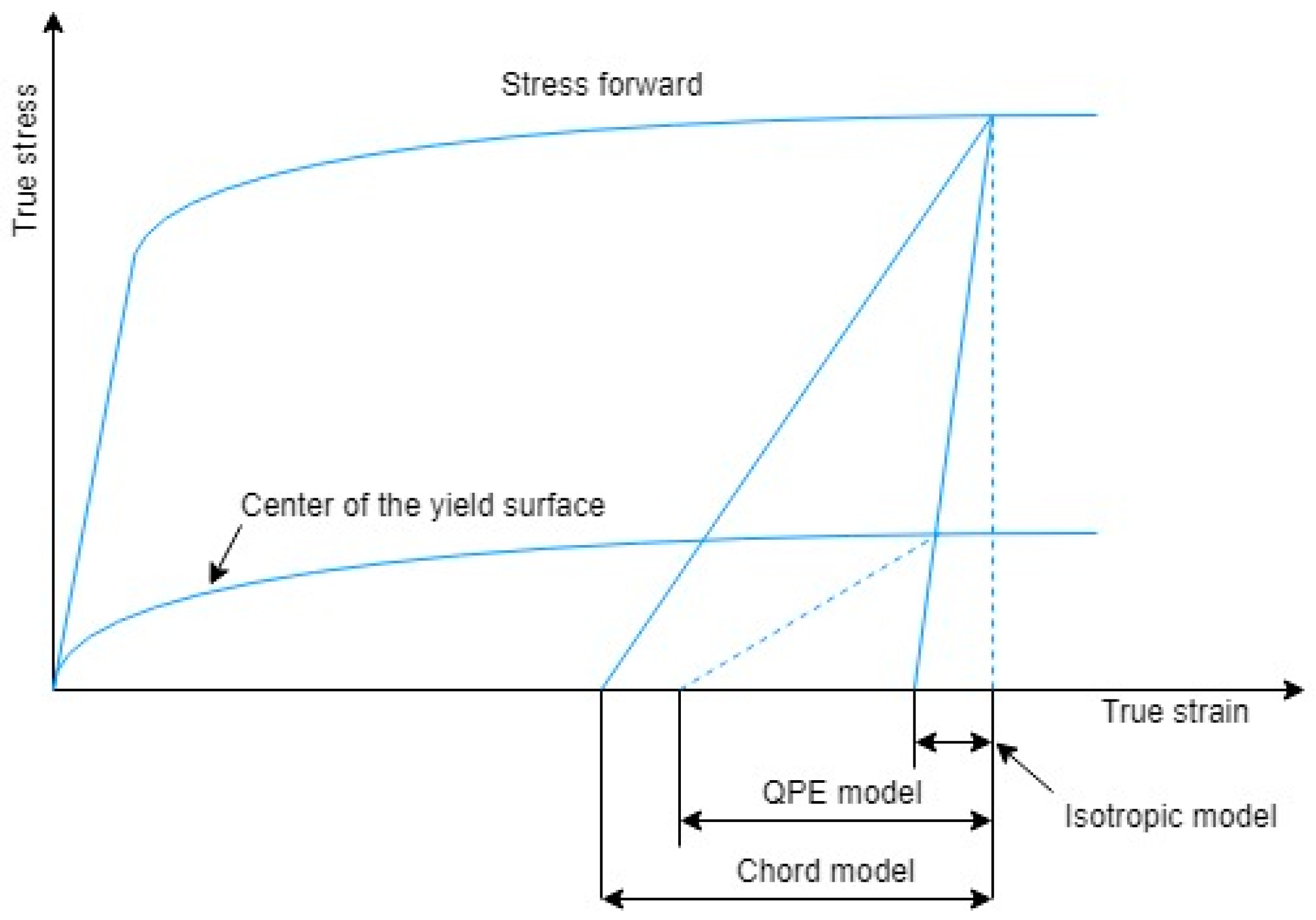
The new unloading elastic modulus is measured as a straight line between the stress forward and the non-zero residual stress.

(2)

Nonlinear regression analysis is used to fit the new model, which is a function of plastic strain.

(3)

The implementation of the new model is combined with von Mises yield criteria in finite element software.

(4)

The numerical integration of the algorithm stress update is implemented as an implicit integration.

(5)

The new model implements two types of nonlinear hardening models, the isotropic model and the combined hardening model, for comparative purposes.

(6)

A shell element is used with reduced integration (S4R) due to its efficiency in sheet metal simulation under plane stress conditions.

(7)

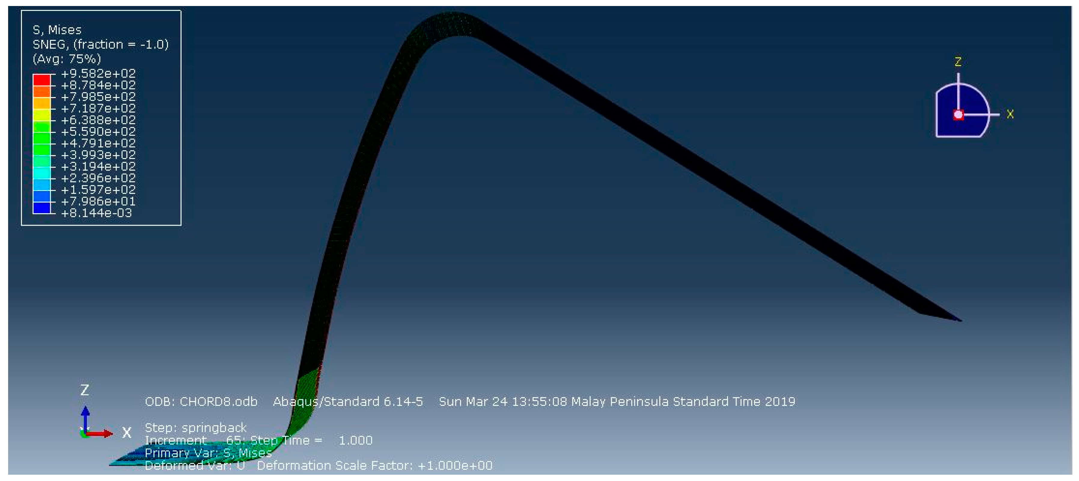
The extended Chord model was verified by comparing the U-draw bending of DP780 with the pre-strain result, which is available in the Numisheet benchmark 2011.

2. Methods

In this section, the methodology of the extended Chord model, the constitutive model, and the numerical integration are described in detail.

2.1. New Model Assumption and Statistical Analysis

Figure 1, regarding DP780, shows that the responses of the stress-strain curve in the unloading path are slightly curved until a certain point of strain recovery in non-zero residual stress. For the isotropic hardening model, the strain recovery or unloading stage occurs between the forward stress and zero stress with original elastic moduli. The zero stress is the center of the yield surface for the isotropic hardening model. The result of the QPE model shows that the strain recovery is positive, instead of there being zero residual stress, at the center of the bounding yield surface. Therefore, it was necessary to extend the Chord model to be able to reproduce strain recovery under positive residual stress. The unloading elastic modulus measured the degradation using a straight line from the forward stress, with the equivalent plastic strain, to the center of the yield surface at a certain point of strain recovery. Also, the extended Chord elastic modulus was measured in three ranges of stress as follows: (1) $0.2 {\sigma }_0\le \sigma \le 0.95 {\sigma }_0$, (2) $0.25 {\sigma }_0\le \sigma \le 0.95 {\sigma }_0$, and (3) $0.3 {\sigma }_0\le \sigma \le 0.95 {\sigma }_0$. The highest part of the range, $0.95 {\sigma }_0$, was due to the high nonlinearity at the start of unloading. The lowest part of the stress range occurred because, in reality, the residual stress occurs at the point between the original elastic modulus and the QPE elastic model after springback terminates. Also, the lowest part of the range is the center of the yield surface, which is the back stress. All unloading elastic moduli were measured in five pre-strains—2%, 4%, 6%, 8%, and 10%—as shown in Figure 1. Finally, the Chord, QPE, and extended Chord models are expressed below, using nonlinear regression analysis between various elastic unloading moduli and plastic strains.

$$E_{Chord}=E_0-\left(E_0-E_a\right)EXP\left(-C\times p\right)$$

(1)

$$E_{QPE}=E_0-E_1(1-EXP\left(D\left({\displaystyle \int }dϵ-d{ϵ}_p\right)\right)$$

(2)

$$E_{Extend Chord}=H_1+\left(H_2\right)EXP\left(-H_3\times P\right)$$

(3)

where $E_{Chord}$, $E_{QPE}$, and $E_{Extend Chord}$ are the Chord, QPE, and extended Chord models’ elastic modulus degradation functions of the equivalent plastic strain $P,$ respectively; $d\epsilon$ is the total strain; $d{ϵ}_p$ is the plastic strain; and $E_a$, $C$, $E_1$, $D$, $H_1$, $H_2$, and $H_3$ are parameters measured by the loading/unloading tensile test of DP780 using nonlinear regression analysis.

For the hardening models, nonlinear isotropic and nonlinear kinematic parameters are measured using the uniaxial tension compression test that was taken from the Numisheet 2011 DP780 benchmark. First, the forward stress is equal to the yield stress plus back stress plus isotropic stress. Thus, the yield stress is constant, and the isotropic and kinematic stress can be changed by a certain value to obtain the forward stress. For example, if the nonlinear kinematic hardening model or the back stress is 30%, then the nonlinear isotropic stress is 70% of the forward stress minus yield stress. The back stress is the center of the yield surface, which is the final stress and strain recovery. Also, the elastic modulus’ degradation depends on the center of the yield surface, because it is measured from the forward stress to the center of the yield surface. Finally, all parameters of the nonlinear isotropic and kinematic hardening models were computed using nonlinear regression analysis to fit the models, as shown in

Table 1. Mechanical properties of DP780 parameters of the varies elastic models and hardening models.

DP780	${\mathit{E}}_{\mathbf{0}}$(MPa)		$\mathit{\nu }$		${\mathit{\sigma }}_{\mathit{U}\mathit{T}\mathit{S}}$(MPa)		${\mathit{\sigma }}_{\mathit{Y}}$(MPa)
	198,800		0.3		944		454
Chord Model	$Q$		$b$		$E_a$ (MPa)		$\mathrm{C}$
	460.7		39.7		152,100		96.5
QPE Model	$Q_B$ (MPa)	$b$	$Q_I$ (MPa)	$H_B$	$E_1$ (MPa)	$\mathrm{D}$	${\gamma }_B$
	431.62	39.7	96.9	17,135.3	95,000	254	39.7
Extended Model	$Q$ (MPa)	$b$	$H_1$	$H_2$	$H_3$	$H$	$\gamma$
(0.3% $\mathit{\sigma }$)	335.7	39.7	165,407	33,083	64.59	4673.86	39.7
(0.25% $\mathit{\sigma }$)	350.2	39.7	163,271	35,291.7	70.5	3543.6	39.7
(0.2% $\mathit{\sigma }$)	383.6	39.7	161,040.9	37,577.7	77.3	3115.9	39.7

.

2.2. Constitutive Models

In this section, constitutive models are evaluated with the Chord, QPE, and the extended models to predict springback. The three models, with their hardening model, were implemented in user subroutine defined material (UMAT Abaqus implicit integration). The yield surfaces were von Mises with two types of hardening models under plane stress conditions. The nonlinear combined isotropic–kinematic von Mises yield surface was selected for the extended and the QPE models. The nonlinear isotropic von Mises yield surface was selected for the Chord model. Both kinds of von Mises hardening models can be expressed by the following equations, respectively:

$${\left({\sigma }_{xx}-{\alpha }_{xx}\right)}^2+{\left({\sigma }_{yy}-{\alpha }_{yy}\right)}^2-{\left({\sigma }_{xx}-{\alpha }_{xx}\right)}^2\times {\left({\sigma }_{yy}-{\alpha }_{yy}\right)}^2+2\ast {\left({\sigma }_{xy}-{\alpha }_{xy}\right)}^2={(R\left(P\right))}^2$$

(4)

$${\left({\sigma }_{xx}\right)}^2+{\left({\sigma }_{yy}\right)}^2-{\left({\sigma }_{xx}\right)}^2\ast {\left({\sigma }_{yy}\right)}^2+2\ast {\left({\sigma }_{xy}\right)}^2=R{\left(P\right)}^2$$

(5)

where ${\sigma }_{xx}$ and ${\sigma }_{yy}$ are stress tensors in the x and y directions, respectively; ${\sigma }_{xy}$ is the shear stress in the plane stress; $R{\left(P\right)}^2$ is the size of the yield surface as a function of the equivalent plastic strain, which is expressed as $P$; ${\alpha }_{xx}$ and ${\alpha }_{yy}$ are the back stress or the center of the yield surface in the x and y directions, respectively; and ${\alpha }_{xy}$ is the back stress of the shear stress.

The size of the yield surfaces for the Chord model and the extension of the chord model can be computed using the following equation:

$$R\left(P\right)={\sigma }_y+Q\ast \left(1-EXP\left(-b\ast P\right)\right)$$

(6)

where ${\sigma }_y$ is the initial yield stress, $Q$ and $b$ are parameters measured from uniaxial tensile test to fit the equation, and $P$ is the equivalent plastic strain.

The size of the inner yield surface and the bounding yield surface can be computed using the following equations, respectively:

$$R_B\left(P\right)={\sigma }_y+Q_B\ast \left(1-EXP\left(-b\ast p\right)\right)$$

(7)

$$R_I\left(P\right)={\sigma }_y+Q_I\ast \left(1-EXP\left(-b\ast p\right)\right)$$

(8)

where $R_B\left(P\right)$ is the size of the bounding yield surface, $Q_B$ is the parameter of the bounding yield surface, $R_I\left(P\right)$ is the size of the inner yield surface, and $Q_I$ is the parameter of the inner yield surface.

2.3. Stress Integration

In this part, the Chord, QPE, and extended Chord models are described with their implicit numerical integration. Both the QPE and extended models use the combined isotropic–kinematic von Mises yield criteria from Equation (4). The Chord model uses the isotropic von Mises yield criteria from Equation (5) without the Chaboche model. The Chord model and extended model use one yield surface. The QPE model uses two surfaces: the first is the inner yield surface that describes linear unloading, and the other is the bounding yield surface or external yield surface that describes nonlinear unloading.

2.3.1. Elastic State Loading and Unloading

In elastic state loading and unloading, the extended model and QPE model share the same equation for the stress-strain relationship. To compute the trial stress, we used Hooke’s law with the original elastic modulus or constant elastic modulus. The relationship between stress and strain is in an incremental form and can be computed using the following equation:

$$\Delta \sigma =D:\Delta \epsilon$$

(9)

where $\Delta \sigma$ is stress the stress increase, $D$ is the elastic stiffness matrix function of the original elastic modulus, and $\Delta \epsilon$ is the strain increase.

For the Chord model, the trial stress was computed using Hooke’s law as a function of the Chord model. The stress-strain relationship is presented in an incremental form and can be computed using the following equation:

$$\Delta \sigma =D_{Chord}:\Delta ϵ$$

(10)

where $D_{Chord}$ is the Hooke’s law function of the Chord elastic model in Equation (1).

In this case, the equivalent von Mises trial stress does not match the size of the yield surface, and no plastic deformation occurs.

2.3.2. Elastic State Unloading and Reloading

In this case, the equivalent plastic strain is greater than zero, and the equivalent trial stress is less than the size of the yield surface. In this mode for the Chord model, the trial stress can be computed using Equation (8). For the extended Chord model, the elastic stiffness matrix is a function of the extended Chord model from Equation (3), instead of using original elastic modulus. The trial stress can be computed using the following equation:

$$\Delta \sigma =D_{Extend Chord model}:\Delta ϵ$$

(11)

where $D_{Extend Chord model}$ is the Hooke’s law function of the extended Chord elastic model from Equation (3).

In the QPE model, two stages occur during the iteration of the stress increase in unloading and reloading. For the first stage, the equivalent trial stress computed by Equation (7) is less than the size of the inner yield surface and the plastic strain is greater than zero. For the second stage, the equivalent trial stress is greater than the size of the inner yield surface and less than the size of the bounding yield surfaces. Both the sizes of the inner and bounding yield surface are constant, and the inner yield surface translates until it is in contact with the bounding yield surface according to the following equation:

$$\Delta {\alpha }_I=\Delta \mu (\left(\frac{R_B\left(P\right)-R_I\left(P\right)}{R_I\left(P\right)}\right)\ast {\sigma }_I-\left(\frac{R_B\left(P\right)}{R_I\left(P\right)}\right)\ast {\alpha }_I+{\alpha }_B)$$

(12)

where $\Delta {\alpha }_I$ is the increase in the back stress of the inner yield surface, ${\sigma }_I$ is the stress at the start of the increase, ${\alpha }_I$ is the back stress of the inner yield surface at the start of the increase, ${\alpha }_B$ is the back stress of the bounding yield surface at the start of the increase, and $\Delta \mu$ is an unknown nonlinear scalar.

In the QPE model in the second stage, the new trial stress can be computed using the Hooke’s law function of the QPE elastic model as follows:

$$\Delta \sigma =D_{QPE}:\Delta \epsilon$$

(13)

where $D_{QPE}$ is the elastic stiffness matrix function of the QPE elastic model from Equation (2).

To find the unknown nonlinear scalar $\Delta \mu$ by substitution, Equations (11) and (12) can be computed using Equation (4), rather than applying the Newton Raphson method to find the solution.

2.3.3. Plastic State

The plastic state occurs when the equivalent trial stress is outside of the size of the yield surface and the trial stress project. Return mapping of stress must be applied to ensure the stress occurs on the yield surface and to correct the plastic strain increase. In the case of using an isotropic yield surface (Chord model), the stress and plastic and elastic strains are updated. The yield surface is expanded without translation, and the Chaboche model is not applied. When using a combined hardening model (QPE and extended Chord model), the stress, back stress, plastic strain, and elastic strain must be updated. The translation of the yield surface moves to the center (back stress) of the yield surface and is expanded by the isotropic hardening model simultaneously. The update of the back stress in incremental form, which is considered a Chaboche model [19], was used according to

$$\Delta \propto =H\ast P\ast N-\gamma \ast \alpha \ast P$$

(14)

$$N=\frac{\left(\mathsf{\sigma }-\mathsf{\alpha }\right)}{\Vert \left(\mathsf{\sigma }-\mathsf{\alpha }\right)\ast \left(\mathsf{\sigma }-\mathsf{\alpha }\right)\Vert }$$

(15)

where $\Delta \propto$ is the back stress for the extended Chord model, $H$ and $\gamma$ are the parameters of the center of the yield surface, $N$ is the flow direction of the stress, and $P$ is the plastic strain increase after return mapping is applied using Newton Raphson method.

The isotropic incremental form is the same as the back stress, but there is a ratio of their parameters, followed as Chaboche model according to

$$\Delta R=b\ast (Q-R\left(P)\right)\ast P$$

(16)

where $Q$ and $b$ are the same parameters of the size of the yield surface in Equation (6) [19].

For the QPE model, the bounding surface is translated and expanded according to the Chaboche model, which is expressed as

$$\Delta {\alpha }_B=H_B\ast P\ast N-{\gamma }_B\ast {\alpha }_B\ast P$$

(17)

$$\Delta R_B=b\ast \left(Q_B-R_B\left(P\right)\right)\ast P$$

(18)

where $\Delta {\alpha }_B$ is the back stress increase of the bounding surface, $H_B$ is the parameter of the bounding surface, ${\gamma }_B$ is the saturated parameter, ${\alpha }_B$ is the back stress of the bounding surface at the end of the increase, $\Delta R_B$ is the increase in the size of the bounding yield surface, $Q_B$ is the parameter of the bounding surface, and $R_B\left(P\right)$ is the current size of the yield surface.

3. Application

All parameters of the extended Chord model, size of yield surface, and back stress were computed using the Newton Raphson method for a uniaxial tensile test that were taken from the Numisheet 2011 benchmark for DP780 sheet steel to fit all models.

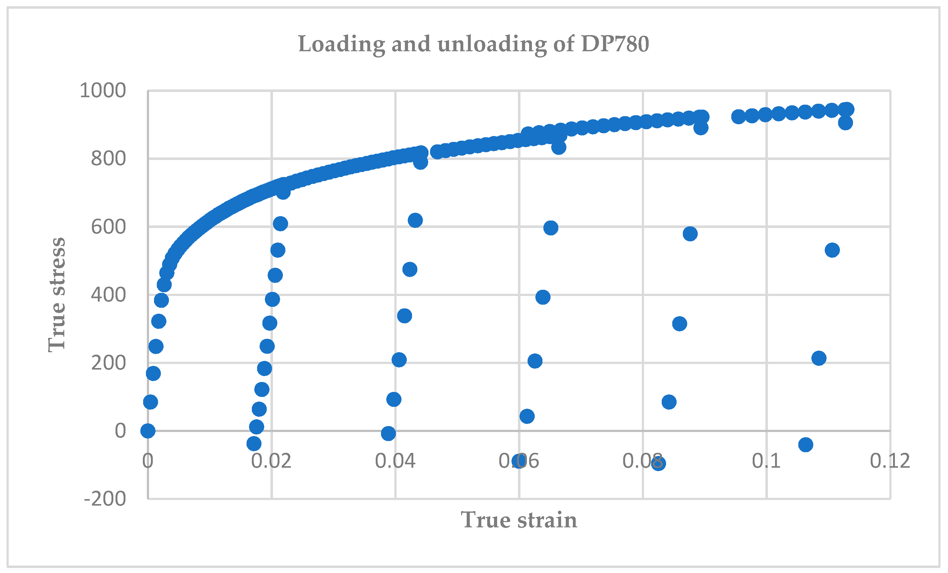
3.1. Description of Stress-Strain Curve of DP780 Sheet Steel

In this study, a 1.4-mm-thick, 380-mm-long, and 30-mm-wide piece of DP780 sheet steel was selected from the Numisheet 2011 benchmark experiment. Rectangular sheet specimens as received had already been prepared. Five-cycle loading, unloading, and reloading with certain plastic strains, 2%, 4%, 6%, 8%, or 10%, was tested using an Instron (Model 8801) universal material testing machine.

3.2. Finite Element Simulation to Evaluate New Model

The algorithm for stress integration of the extended Chord model was implemented into UMAT implicit integration using Abaqus software. The S4R shell element, with four nodes for reducing integration, was selected due to its robust accuracy and to reduce the time required for sheet metal forming simulation. The elements applied were 4 mm² and we used 5467 elements. The punch, die, and holder were modeled as rigid bodies. All hardening models had 5 layers. The QPE model simulation required 12 h, and the Chord model and the extended Chord model required 6 h each using one workstation processor.

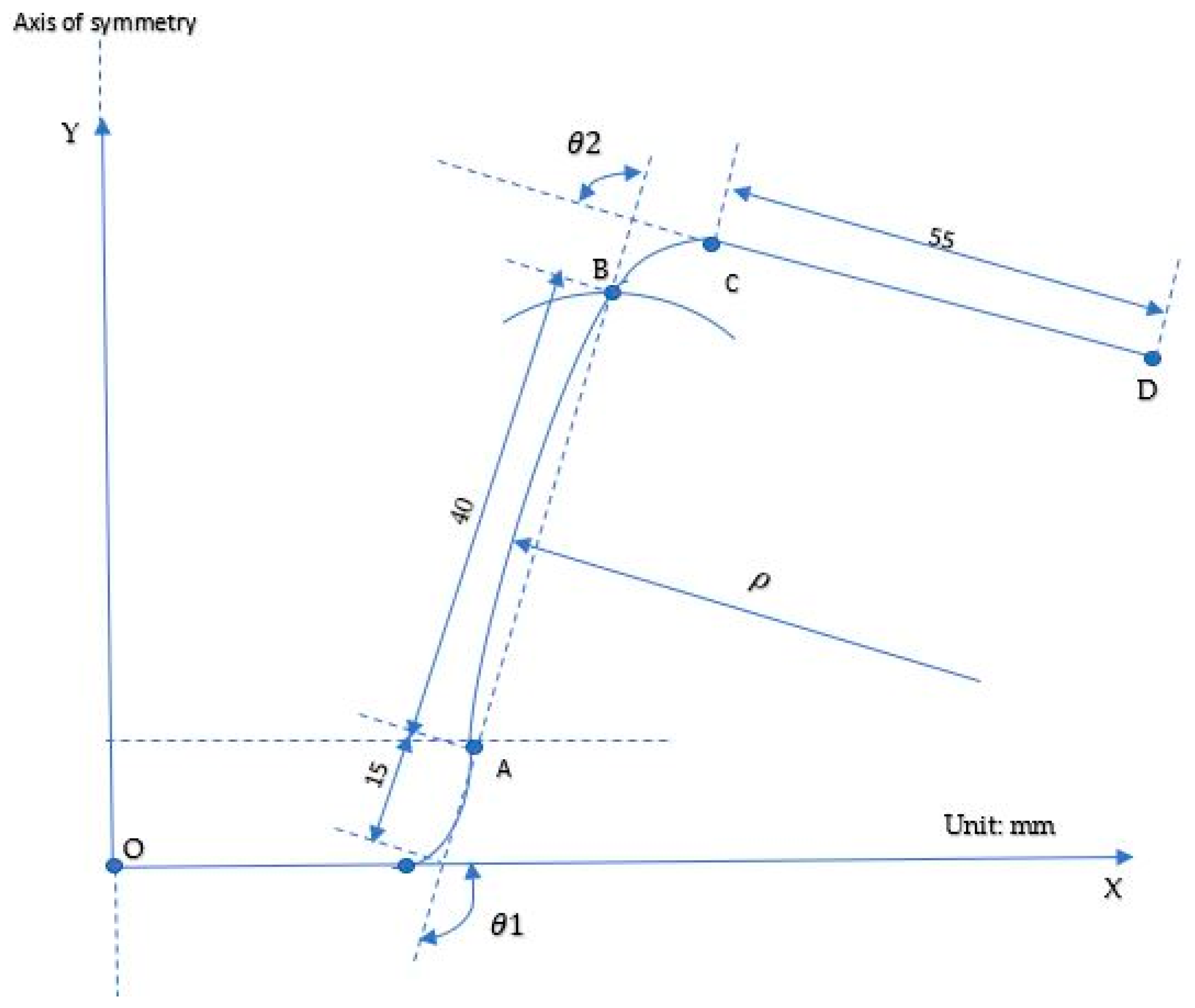
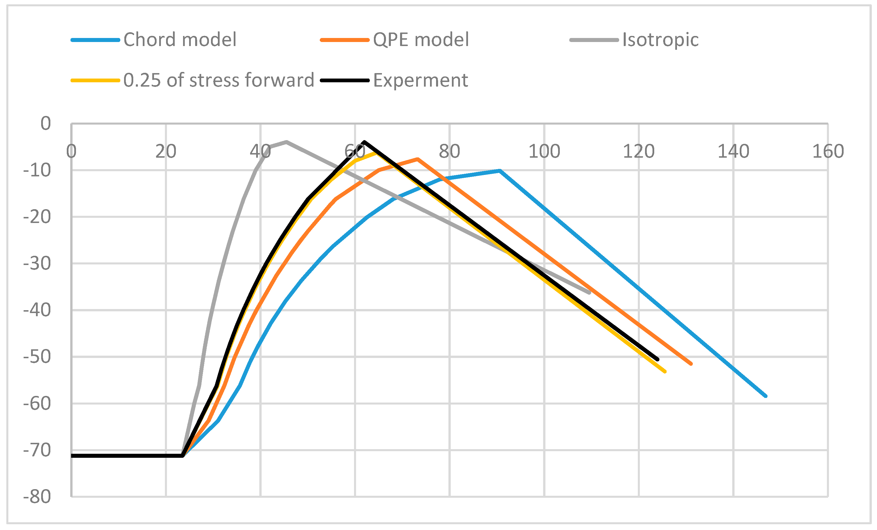
3.3. Draw-Bending Tests to Predict Springback

The dimensions of the punch, holder, and die used to draw the U bending are shown in Figure 2, and the three parameters for the springback simulation used to evaluate the new model are illustrated in Figure 3. The holding force applied was 2940 KN, and the friction coefficient between the sheet and tools was 0.1 with a hard coefficient. The speed of the punch was 1 mm/s.

4. Discussion

Abaqus software has two types of hardening models that can be used to simulate springback. The first method is the isotropic hardening model that uses the original elastic modulus. This kind of hardening model’s center of the yield surface is zero in stress space during sheet metal deformation. The unloading stage started when the die, punch, and holder were removed. In this stage, the stress and strain recovery relaxes until the balance point (the center of the yield surface) of the residual stress is reached. In the isotropic hardening model, the strain recovery is less than the true strain recovery measurement, due to the large slope of the elastic modulus. For the second method, the nonlinear isotropic and kinematic hardening models are combined with the original elastic modulus. In this method, the center of the yield surface is equal to the back stress, which is greater than zero and leads to less strain recovery than in the isotropic hardening model. The combined hardening model uses 100% back stress and 0% isotropic stress, which leads to a very large positive back stress (center of the yield surface) and very small strain recovery. Thus, both hardening models available in Abaqus software overestimate springback and predict less strain recovery than in reality. This measurement is supported by similar findings reported by Zang et al. [20].

From the previous discussion, the main factors that affect springback or strain recovery prediction accuracy using finite element software are the measurement of the elastic modulus degradation and the size of the yield surface [3]. Thus, if the elastic modulus and the center of the yield surface decrease, the strain recovery increases. The Chord model with the isotropic hardening model overestimate compared with experimental measurements due to the lower measurement of the elastic moduli’s degradation with zero residual stress, which led to a larger strain recovery than for actual strain recovery [17]. The QPE model is more accurate than the Chord model due to the size of the yield surface, which leads to non-zero residual stress and larger elastic modulus degradation, with the center of the yield surface 18% higher in terms of forward stress than the Chord model [17,18,21,22,23]. Figure 4 depicts the main differences in springback prediction between the isotropic hardening model with the original elastic modulus, the Chord model, and the QPE model. We assumed that the extended Chord model was able to predict springback more accurately than the Chord and QPE models because the elastic modulus degradation and the size of yield surface consider where location of the balance point of strain recovery. The extended model is not as complicated as the Chord and QPE models, because it only uses one yield surface and is easy to implement in finite element software user subroutines.

Isotropic, Chord, QPE, and extended models were implemented in Abaqus to verify the accuracy of the extended model. According to the simulation results in

Table 2. Measurement of the parameters and errors of springback simulation.

Parameters of Springback	Experiment	Isotropic Model	QPE	Chord Model	20% $\mathit{\sigma }$	25% $\mathit{\sigma }$	30% $\mathit{\sigma }$
$\theta 1$	115.8	103.25	119.4	105.26	120.5	116.3	111.03
$\theta 2$	79.2	76.5	83.3	88.33	84.2	78.67	77.1
$\rho$	118.2	190.49	108	82.65	105.26	117	131.89
Errors
$\theta 1$	0%	10.83%	3.1%	9.1%	4%	1.43%	4.1%
$\theta 2$	0%	3.4%	5.17%	11.48%	6.31%	2.7%	3.65%
$\rho$	0%	61.15%	8.6%	30%	10.94%	2.6%	11.5%

, the results for obtaining the balance point (springback) were logical. The strain recovery simulation was set up for several constitutive models from very large to small: Chord, QPE, the extended model, and isotropic models, respectively. Thus, the strain recovery of the extended model was between that predicted by the QPE model and that by the isotropic model, which was the strain recovery nearest to the balance point compared with the experimental measurement, as shown in Figure 5.

The accuracy and the errors of the measurements of the three parameters of springback predication for all models are provided in Table 2. The errors of the isotropic model were 10.83% of $\theta 1$, 3.4% of $\theta 2$, and 61.15% of $\rho$. The errors of the Chord model were 9.1% of $\theta 1$, 11.48% of $\theta 2$, and 30% of $\rho$. The errors of the QPE model were 9.1% of $\theta 1$, 11.48% of $\theta 2$, and 30% of $\rho$. The extended model underestimated the parameters compared with the other models if the elastic modulus’ degradation with the center of the yield surface was considered. The accuracy of the appropriate center of the yield surface was 25% of the forward stress with their elastic modulus’ degradation. Therefore, the errors of the extended model’s simulation of 25% of the forward stress were minimized to 1.43% of $\theta 1$, 2.7% of $\theta 2$, and 2.6% of $\rho$ compared with the other models. The simulation of the appropriate extended Chord model of 25% of the forward stress using Abaqus is shown in Figure 6. The validation of the current model for other types of advanced high-strength steel sheet depends on its mechanical properties and the amount of the residual stress in the strain recovery stage. Thus, to choose the appropriate model for other advanced high-strength steel sheets, the variation of the elastic model degradation with different sizes of yield surfaces and simulations must be examined.

5. Conclusions

In this work, we extended and devolved the Chord model using nonlinear combined hardening models with only one yield surface. The numerical integration was completely implicit, and was implemented in user-defined material subroutine (UMAT) under plane stress conditions. By using one yield surface with a combined hardening model to control the size of the yield surface and elastic modulus degradation, the simulated strain recovery prediction was more accurate compared with the other models. The extended model could be implemented in finite element software using one von Mises yield surface. The verified extended model, when compared with experimental measurements, showed that the approximate stress-strain curve behavior in the unloading path, which was used to obtain an accurate balance point, affected the accuracy simulation in predicting springback when the elastic degradation and size of the yield surface were considered.

The parameters of the extended model, Chord model, QPE model, nonlinear isotropic model, and nonlinear kinematic model were obtained from a uniaxial tension compression test (Benchmark 2011) of DP780 using nonlinear regression analysis. The simulation of the stress-strain curve showed that the parameters were better able to reproduce the stress-strain curve. The QPE model was good at reproducing the nonlinear unloading path but was a more complicated constitutive model to implement.

Finally, we simulated the Benchmark 2011 U-draw bending of DP780 high-strength steel sheet without pre-strain. The result showed that our model provides improved springback prediction when the elastic modulus degradation and the size of the center of the yield surface are considered.

References

1. Lems, W. The Change of Young’s Modulus after Deformation at Low Temperature and Its Recovery. Ph.D. Thesis, Delft University of Technology, Delft, The Netherlands, 1963. [Google Scholar]
2. Morestin, F.; Boivin, M. On the necessity of taking into account the variation in the Young modulus with plastic strain in elastic-plastic software. Nucl. Eng. Des. 1996, 162, 107–116. [Google Scholar] [CrossRef]
3. Yoshida, F.; Uemori, T.; Fujiwara, K. Elastic-plastic behavior of steel sheets under in plane cyclic tension-compression at large strain. Int. J. Plast. 2002, 18, 633–659. [Google Scholar] [CrossRef]
4. Cleveland, R.M.; Ghosh, A.K. Inelastic effects on springback in metals. Int. J. Plast. 2002, 18, 769–785. [Google Scholar] [CrossRef]
5. Yang, M.; Akiyama, Y.; Sasaki, T. Evaluation of change in material properties due to plastic deformation. J. Mater. Process. Technol. 2004, 151, 232–236. [Google Scholar] [CrossRef]
6. Luo, L.; Ghosh, A.K. Elastic and inelastic recovery after plastic deformation of DQSK steel sheet. J. Eng. Mater. Technol. 2003, 125, 237–246. [Google Scholar] [CrossRef]
7. Fei, D.; Hodgson, P. Experimental and numerical studies of springback in air v bending process for cold rolled TRIP steels. Nucl. Eng. Des. 2006, 236, 1847–1851. [Google Scholar] [CrossRef]
8. Pérez, R.; Benito, J.A.; Prado, J.M. Study of the inelastic response of TRIP steels after plastic deformation. ISIJ Int. 2005, 45, 1925–1933. [Google Scholar] [CrossRef]
9. Mendiguren, J.; Cortés, F.; Gómez, X.; Galdos, L. Elastic behaviour characterisation of TRIP 700 steel by means of loading–unloading tests. Mater. Sci. Eng. 2015, 634, 147–152. [Google Scholar] [CrossRef]
10. Ghaei, A.; Green, D.E. Numerical implementation of Yoshida-Uemori two-surface plasticity model using a fully implicit integration scheme. Comput. Mater. Sci. 2010, 48, 195–205. [Google Scholar] [CrossRef]
11. Ghaei, A.; Green, D.E.A. Taherizadeh, Semi-implicit numerical integration of Yoshida-Uemori two-surface plasticity model. Int. J. Mech. Sci. 2010, 52, 531–540. [Google Scholar] [CrossRef]
12. Taherizadeh, A.; Ghaei, A.; Green, D.E.; Altenhof, W.J. Finite element simulation of springback for a channel draw process with drawbead using different hardening models. Int. J. Mech. Sci. 2009, 51, 314–325. [Google Scholar] [CrossRef]
13. Ghaei, A. Numerical simulation of springback using an extended return mapping algorithm considering strain dependency of elastic modulus. Int. J. Mech. Sci. 2012, 65, 38–47. [Google Scholar] [CrossRef]
14. Zang, S.L.; Lee, M.G.; Kim, J.H. Evaluating the significance of hardening behavior and unloading modulus under strain reversal in sheet springback prediction. Int. J. Mech. Sci. 2013, 77, 194–204. [Google Scholar] [CrossRef]
15. Yu, H.Y. Variation of elastic modulus during plastic deformation and its influence on springback. Mater. Des. 2009, 30, 846–850. [Google Scholar] [CrossRef]
16. Ghaei, A.; Green, D.E.; Thuillier, S.; Morestin, F. On the use of cyclic shear, bending and uniaxial tension–compression tests to reproduce the cyclic response of sheetmetals. Proc. Inst. Mech. Eng. 2015, 229, 453–462. [Google Scholar] [CrossRef]
17. Lee, J.; Lee, J.-Y.; Barlat, F.; Wagoner, R.H.; Chung, K.; Lee, M.-G. Extension of quasi plastic–elastic approach to incorporate complex plastic flow behavior—Application to springback of advanced high-strength steels. Int. J. Plast. 2013, 45, 140–159. [Google Scholar] [CrossRef]
18. Sun, L.; Wagoner, R.H. Complex unloading behavior: Nature of the deformation and its consistent constitutive representation. Int. J. Plast. 2011, 27, 1126–1144. [Google Scholar] [CrossRef]
19. Chaboche, J.L. Time-Independent Constitutive Theories for Cyclic Plasticity. Int. J. Plast. 1986, 2, 149–188. [Google Scholar] [CrossRef]
20. Zang, S.L.; Liang, J.; Guo, C. Constitutive model for spring-back prediction in which the change of Young’s modulus with plastic deformation is considered. Int. J. Mach. Tools Manuf. 2007, 47, 1791–1797. [Google Scholar] [CrossRef]
21. Green, D.E.; Ghaei, A.; Aryanpour, A. Springback simulation of advanced high strength steels considering nonlinear elastic unloading-reloading behaviour. Mater. Des. 2015, 88, 461–470. [Google Scholar]
22. Zajkani, A.; Hajbarati, H. Investigation of the variable elastic unloading modulus coupled with nonlinear kinematic hardening in springback measuring of advanced high-strength steel in U-shaped process. J. Manuf. Process. 2017, 25, 391–401. [Google Scholar] [CrossRef]
23. Wagoner, R.H.; Chen, Z.; Gandhib, U.; Leec, J. Variation and consistency of Young’s modulus in steel. J. Mater. Process. Technol. 2016, 227, 227–243. [Google Scholar]
Figure 1. Stress-strain curve in tension compression test.
Metals 09 00511 g001
Figure 2. Dimensions of the punch, die, and holder of U-draw bending.
Metals 09 00511 g002
Figure 3. Parameters used for springback measurement.
Metals 09 00511 g003
Figure 4. Strain recovery or springback in different models.
Metals 09 00511 g004
Figure 5. Springback profile of the different hardening models compared in our experiment.
Metals 09 00511 g005
Figure 6. Springback simulation for 25% of stress forward.
Metals 09 00511 g006