Article

Prediction of Isotropic Rough Surface Directional Spectral Emissivity with Surface-Morphology-Dependent Modelling

1
School of Mechanical Engineering, Shandong University, Jinan 250061, China
2
Key National Demonstration Center for Experimental Mechanical Engineering Education/Key Laboratory of High Efficiency and Clean Mechanical Manufacture of MQE, Shandong University, Jinan 250061, China
*
Author to whom correspondence should be addressed.
Metals 2023, 13(10), 1679; https://doi.org/10.3390/met13101679
Submission received: 6 September 2023 / Revised: 25 September 2023 / Accepted: 26 September 2023 / Published: 30 September 2023

Abstract

:
The surface directional spectral emissivity of rough metal surfaces in industry is of concern in infrared temperature measurement. In this research, the height and slope possibility density functions are introduced as variables, and the directional spectral emissivity of isotropic rough surface is modelled accordingly. The model is designed to derive the directional spectral emissivity of rough metal surfaces from the surface morphology (possibility distribution of the height and slope) and the material property parameters (refractivity). Then, a sandblasted surface is taken as a case study. The sandblasted surface morphology is measured. A Polynomial surface is proposed to describe the sandblasted surface morphology and is compared with a Gaussian surface and a Cox–Munk surface. Finally, the directional spectral emissivity measurement and infrared temperature measurement are conducted. It is shown that the predicted directional spectral emissivity and measured temperature with the surface-morphology-dependent isotropic rough surface directional spectral emissivity model have high precision. In this work, the possibility distribution of the height and slope of the surface is introduced as independent variables to provide better accuracy compared to the reported models. In some cases, the error of the infrared temperature measurement could be reduced to 20% (80 degrees, compared to Gaussian surface). This work contributes to improving the accuracy of IR temperature measurement of rough surfaces.

1. Introduction

Infrared-related measurement of rough surfaces including sandblasted surfaces and casted surfaces has been widely applied in machining and other metal-related processes in the industry [1,2,3]. An infrared thermometer is introduced for on-time temperature measurement in the dry cutting of AISI 1045 [4]. The results show good coherence with the data measured using thermocouples. Similar research on the milling of Ti-6Al4-V has also been reported [5]. Infrared technology is also used in other metal-related industries. An infrared thermometer is used to monitor the impact damage of different types of composites [6]. Lock-in infrared thermography shows good ability in detecting the impact damage of the specimens. The infrared feature can also be used in coolant flow inside a one-stage metal turbine [7].
Inconel 718 is a hard-to-cut metal material, often inducing high temperatures in the machining process. The temperature measurement of the rough Inconel 718 surface is thus to be carried out. In the field of machining, with Inconel 718 for example, Xu et al. [8] monitored the cutting temperature field during the turning process of Inconel 718 using an infrared thermal camera. The temperature field drawn in the experiment was compared to theoretical results, and the influence of the tool rake angle was studied. Liu et al. [9] applied infrared imaging on the milling of Inconel 718. The thermos image was compared to the predicted temperature as verification. The infrared remote sensing of Inconel 718 was also reported. The temperature sensitivity of the physical properties of laser-metal-deposited Inconel 718 was investigated using infrared measurement [10]. The infrared pyrometer and high-speed infrared camera were introduced to analyse the uniformity of the temperature field of the sample on a Hopkinson bar setup. The strength model of the material as a function of temperature was proposed to guide the finite element simulation. An infrared camera was used in the real-time temperature tracking of Inconel 718 deposition in the laser engineered net shaping process [11]. The infrared camera was also used in the directed energy deposition of Inconel 718 [12]. However, the directional emissivity of these Inconel 718 surfaces is usually roughly set as 0.2, regardless of the surface morphology, which can severely influence the emissivity of the surface and include errors in infrared measurement.
Surface morphology parameters are prescribed according to ISO-25178. The most commonly used parameter in the field of directional spectral emissivity are arithmetic mean deviation Ra [13,14,15], root mean square deviation  R q  [13,14,16], arithmetic mean height  S a  [13,17], and root mean square height  S q  [13,17]. The root mean square gradient  S d q  is also reported and referred to as the most important parameter in the field of infrared emissivity [18,19,20]. Skewness  S s k  and kurtosis  S k u  are also introduced to describe the height and slope of the rough surface in detail [21]. These parameters show certain aspects of the morphology of the surface, but none are sufficient to sketch the full image of the surface.
Other parameters or methods are also used in the field of field of cutting. The 3D frequency information of the single-point diamond turning (SPDT) of a potassium dihydrogen phosphate (KDP) crystal surface is decomposed and analysed with the wavelet transform method [22]. But such a method has not yet been reported in the field of infrared directional spectral emissivity or temperature measurement. Series [21,23] and random series [24,25] of sinusoidal functions are also established to simulate rough surfaces with certain pattern to obtain directional spectral emissivity. The optical constants are used in a modified geometric optics approximation. These methods are more suitable to describe a certain surface with certain pattern rather than the most commonly used rough metal surfaces, and they are not widely accepted. To better show the detail of the rough surface, the height and slope distribution of the rough surface are assumed, and the directional spectral emissivity is modelled. The height and slope distribution of the rough surface are usually assumed to follow Gaussian distributions (Gaussian surface), isotropy [26,27,28,29], or anisotropy [30,31,32]. The rough surface directional spectral emissivity model is extended to a Cox–Munk surface [33] (C-M surface) in order to consider skewness and kurtosis of the surface [21].
However, the directional spectral emissivity of a rough surface is hardly predicted precisely. The rough surface morphology is the base of the optical mechanism of directional spectral emissivity, yet its characterization is barely reported in directional spectral emissivity modelling. The feature of rough surface morphology, including machined surface morphology, does not meet the assumptions of the directional spectral emissivity models. In order to conduct precise infrared measurement or remote sensing on rough surfaces, it is necessary to determine the directional spectral emissivity according to the surface morphology of these rough surfaces [21,23].
In this research, the surface morphology, namely the possibility distribution of the height and slope, is introduced as variables in the form of a possibility density function. The other variable is the material parameter reflectivity n. The isotropic rough surface directional spectral emissivity model is brought up accordingly to predict the directional spectral emissivity  ε . Then, a sandblasted surface is taken as a case study, and its surface morphology is described. It is shown that the infrared temperature measurement error is decreased due to the highly precise prediction of directional spectral emissivity. By measuring and accepting the surface morphology as an input, more information is introduced in the model to specifically sketch the surface, and thus, a better prediction of the emissivity is gained. The framework of this work is shown in Figure 1.

2. Modelling of Isotropic Rough Surface Directional Spectral Emissivity

The directional spectral emissivity of isotropic rough surface modelling is proposed based on the former work of the authors [34]. The rough surface studied in this research is assumed as an isotropic rough surface with the following characteristics:
(1)
The refractive index on the surface and inside the material is irrelevant to spatial direction;
(2)
The surface height and slope are distributed randomly;
(3)
The surface height and slope distribution obey the same probability density function in any direction on the plane.
As the surface is isotropic, any beam could either leave the surface or eventually hit the surface. A beam that hits the surface could either be absorbed or reflected. The optics of isotropic rough surface directional spectral emissivity could thus be expressed separately and combined to derive the directional spectral emissivity wanted.

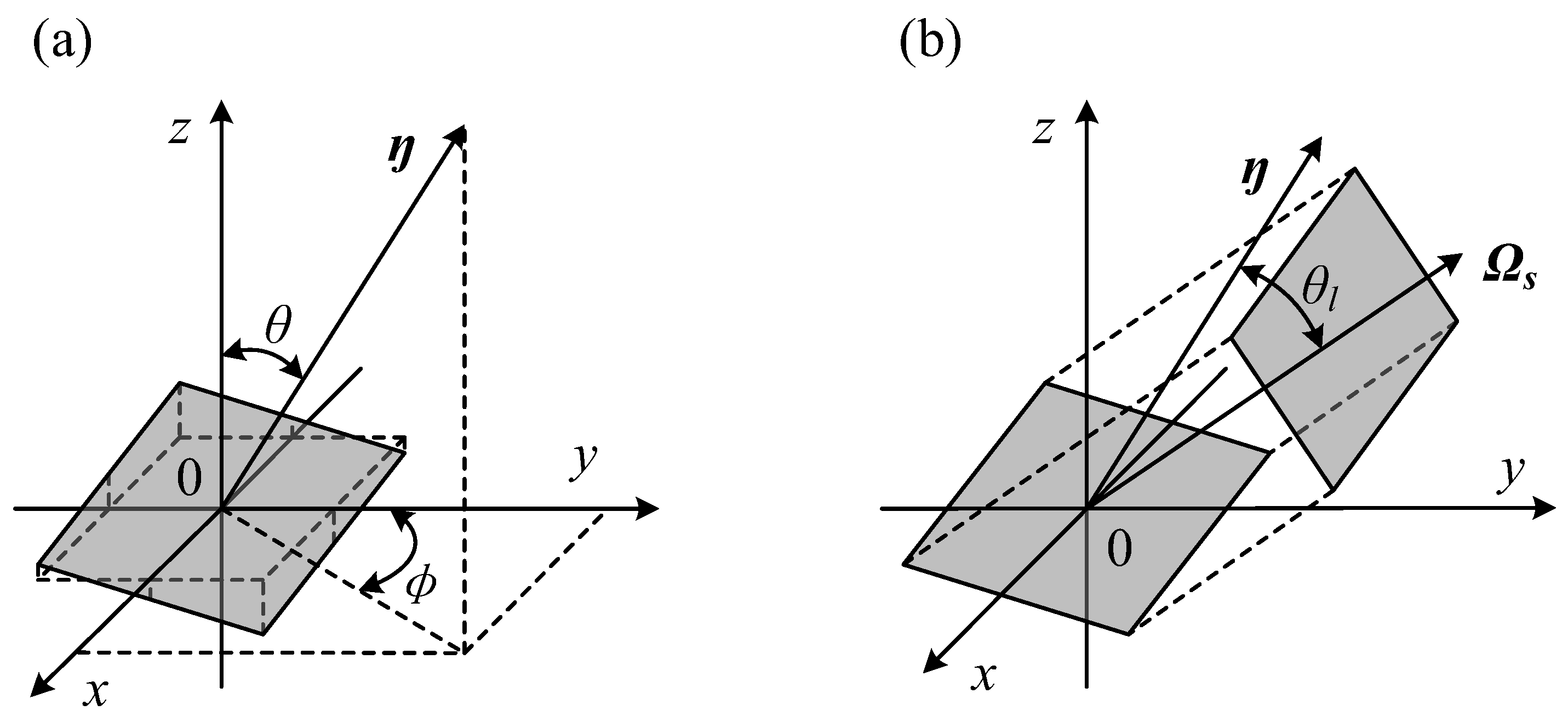
2.1. Derivation of Viewing Possibility Density Function  t ( θ s , p , q )

As shown in Figure 2, assume that the viewing direction Ωs is on the plane yoz. As the rough surface studied in this research is isotropic, this assumption is valid. The surface element normal direction η is expressed as Equation (1),
η = ( p p 2 + q 2 + 1 , q p 2 + q 2 + 1 , 1 p 2 + q 2 + 1 )
where p and q are the slopes of the surface element in the x and y directions, respectively. The same element on the surface could have a different projection area in a different direction and thus have a different contribution to the directional spectral emissivity of the surface. Based on the direction of the element, the area projection coefficient Ap could be expressed as
A p = { η yoz   Ω s = cos ( θ s ) q sin ( θ s ) , q < cot ( θ s ) 0 , q cot ( θ s )
where ηyoz is the component parallel to the plane yoz of vector η, and θs is the viewing angle. As shown in Figure 2b, the area projection coefficient Ap denotes the projection area of the element perpendicular to the viewing direction Ωs, representing how it ‘looks like’ in a certain direction. The element would be shadowed and could not be seen when  q cot ( θ s ) , leading to  A p = 0 .
There is
t ( θ s , p , q ) = A p f ( p ) f ( q ) cot θ s A p f ( p ) f ( q ) d p d q
where  t ( θ s , p , q )  is the viewing possibility density function, and  f ( p )  is the slope possibility density function of the isotropic rough surface.  t ( θ s , p , q )  represents the possibility that a random light beam from the angle  θ s  would hit an element with the normal direction of η. According to the principle of reversibility, it also denotes the proportion of light from an element with a certain direction detected on direction  θ s . Note that the viewing possibility density function  t ( θ s , p , q )  is not a function of  ϕ , which again indicates that the surface is isotropic.

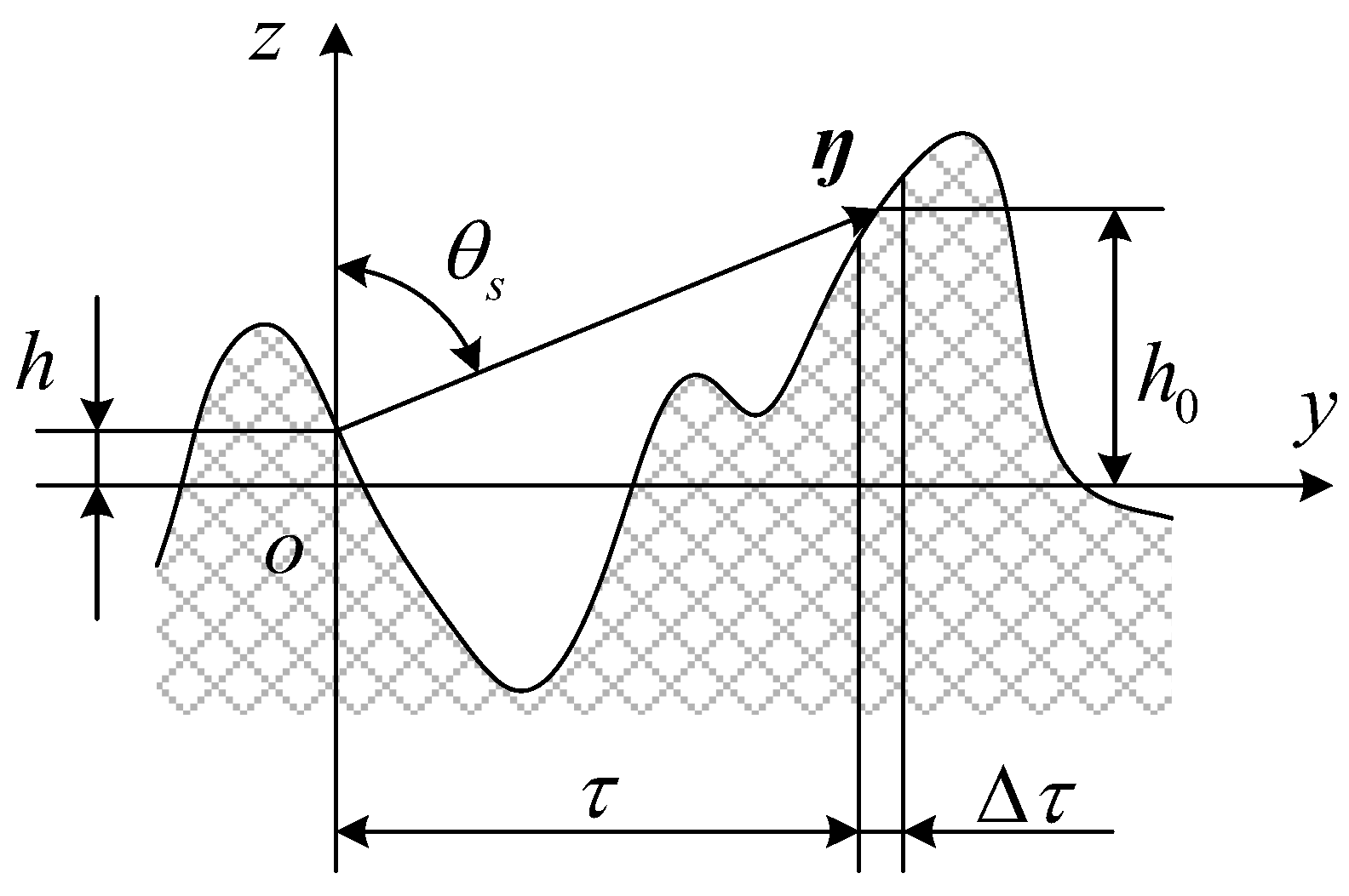
2.2. Derivation of Shadowing Function

Shadowing is an optical process in which the infrared electromagnetic wave emitted from the surface gets blocked by another part of the surface, as shown in Figure 3. The correlation between elements is not significant and can be ignored [35,36,37]. The shadowing function can be expressed using Equation (4) [20,38],
S ( θ s ) = { exp [ 0 P u ( τ ) d τ ] , θ s < π 2 0 , θ s π 2
where the shadowing function  S ( θ s )  is the possibility that the infrared radiation is not blocked. If  θ s π 2 , the wave would certainly be blocked by the surface, making shadowing function  S ( θ s )  = 0. As shown in Figure 3, the physical significance of the intermediate variable Pu(τ) is the possibility that the infrared electromagnetic wave hits the certain element located at y = τ, which is the possibility that the beam is not blocked in  y ( 0 , τ ]  and blocked in  y ( τ , τ + Δ τ ) .
As metal is of good conductivity, the electromagnetic wave is unlikely to penetrate, and the transmission inside the material could be neglected. The following events are defined. Event A: the infrared electromagnetic wave is not blocked in  y ( 0 , τ ] ; event B: the infrared electromagnetic wave hits the surface where  y = τ ; and event C:  q | y = τ > θ s . Event C is a necessary condition of event B. As the correlation between different elements is neglected, there is
P u ( τ ) = P ( B C | A ) = p u B ( τ ) p u C ( τ ) p u A ( τ )
where  p u A ( τ ) p u B ( τ ) , and  p u C ( τ )  are the possibility functions of event A, B, and C, respectively.
The event A possibility function  p u A ( τ )  is expressed using Equation (6),
p u A ( τ ) = p 1 g ( h ) [ h + τ cot ( θ s ) g ( h 0 ) d h 0 ] d h
where  p 1  is the possibility that the infrared electromagnetic wave is not blocked in  y ( 0 , τ ) , and  g ( h )  is the height possibility density function of the isotropic rough surface. The event B possibility function  p u B ( τ )  and the event C possibility function  p u C ( τ )  are described with Equation (7) and Equation (8), respectively.
p u B ( τ ) = p 1 g ( h ) g [ h + τ cot ( θ s ) ] d h
p u C ( τ ) = cot ( θ s ) [ q cot ( θ s ) ] f ( q ) d q

2.3. Derivation of Directional Spectral Emissivity

Based on the previous work of the authors [36], the directional spectral emissivity  ε  can be sketched using Equation (9),
ε = Σ i = 0 ε i
where  ε 0 ε 1 ε 2 , and so on are the zeroth-order component, first-order component, second-order component, etc. There is
ε 0 = cot θ s t ( θ s , p , q ) S ( θ s ) ε l ( n , p , q , θ s ) d p d q
where  ε l ( n , p , q , θ s )  is the local directional spectral emissivity of the surface elements.
There is
ε l ( n , p , q , θ s ) = { n 2 sin 2 ( θ s l ) n 2 cos ( θ s l ) + n 2 sin 2 ( θ s l ) + cos ( θ s l ) cos ( θ s l ) + n 2 sin 2 ( θ s l ) , tan θ s l < n n 2 cos ( θ s l ) n 2 cos ( θ s l ) + n 2 sin 2 ( θ s l ) + cos ( θ s l ) cos ( θ s l ) + n 2 sin 2 ( θ s l ) , tan θ s l n
θ s l = cos 1 ( cos ( θ s ) q sin ( θ s ) 1 + p 2 + q 2 )
where n is the refraction index of the material.  θ s l  is the local viewing angle of the surface elements. The  t ( θ s , p , q )  is the possibility of an element with certain parameters getting detected. The  ε l ( n , p , q , θ s )  is about the directional spectral emissivity of the element. The  S ( θ s )  is the possibility of the element to not be blocked. The integral thus shows the overall effect of the whole surface.
The first-order component is
ε 1 = 0 2 π 0 π θ s i ( θ 1 ) t ( θ s , θ 1 , ϕ 1 ) S ( θ s ) [ 1 ε l ( n , θ 1 , ϕ 1 , θ s ) ] sin θ 1 d θ 1 d ϕ 1
i ( θ 1 ) = cot θ 1 t ( θ 1 , p 1 , q 1 ) [ 1 S ( θ 1 ) ] ε l ( n , θ 1 , ϕ 1 , θ s ) d p 1 d q 1
where the  i ( θ 1 )  part is about the blocked beam emitted from other part of the surface. The first-order component  ε 1  shows the directional spectral emissivity component from the beam reflected once before leaving the surface. Similarly, the second-order component is
ε 2 = 0 2 π 0 π θ s i 2 ( θ 2 ) t ( θ s , θ 2 , ϕ 2 ) S ( θ s ) [ 1 ε l ( n , θ 2 , ϕ 1 ) ] sin θ 2 d θ 2 d ϕ 2
i 2 ( θ 2 ) = cot θ 2 i 1 ( θ 1 ) t ( θ s , θ 1 , ϕ 1 ) [ 1 S ( θ s ) ] [ 1 ε l ( n , θ 1 , ϕ 1 ) ] sin θ 1 d θ 1 d ϕ 1
  i 1 ( θ 1 ) = cot θ 1 t ( θ 1 , p 1 , q 1 ) [ 1 s ( θ 1 ) ] ε l ( n , p 1 , q 1 ) d p 1 d q 1
The third order component and above can be sketched similarly. The matrix method reported by the authors [34] is applied to solve the components  ε i . In this research, the components are considered until  ε i < 10 4 . The matrix method is introduced to numerically compute the directional spectral emissivity, as mentioned in previous work of the authors [36].

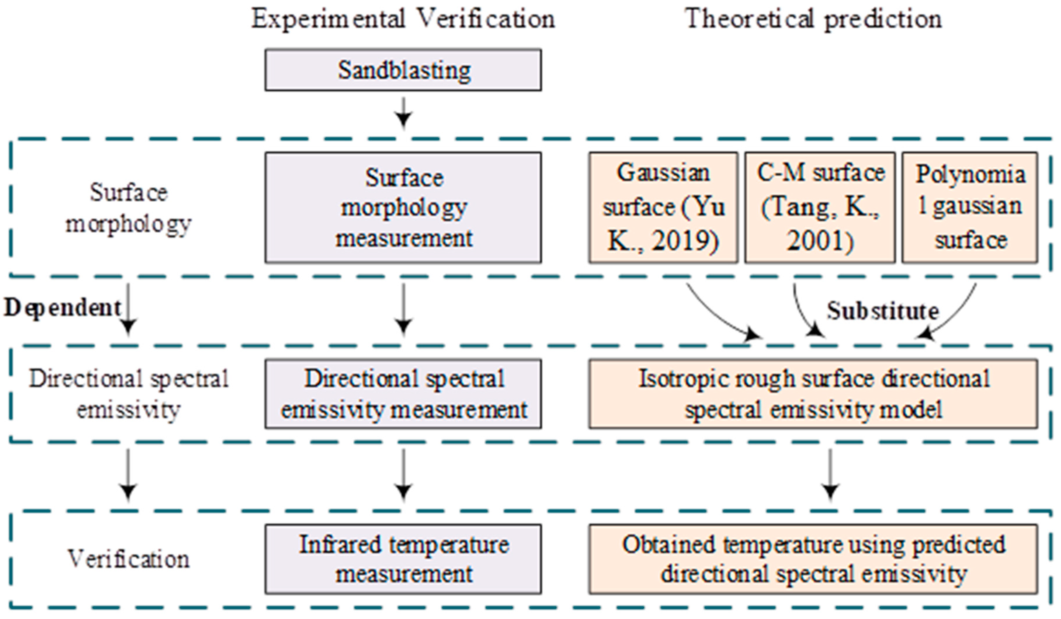
3. Experimental Verification

The case study is applied on sandblasted Inconel 718 samples. The surface morphology is measured with a confocal laser scanning microscope. Each group contains 5 samples to avoid the influence of random factors. The surface height and slope are processed using MATLAB mods and programs. The directional spectral emissivity measurement device is developed. Directional spectral emissivity measurement and infrared temperature measurement are conducted.

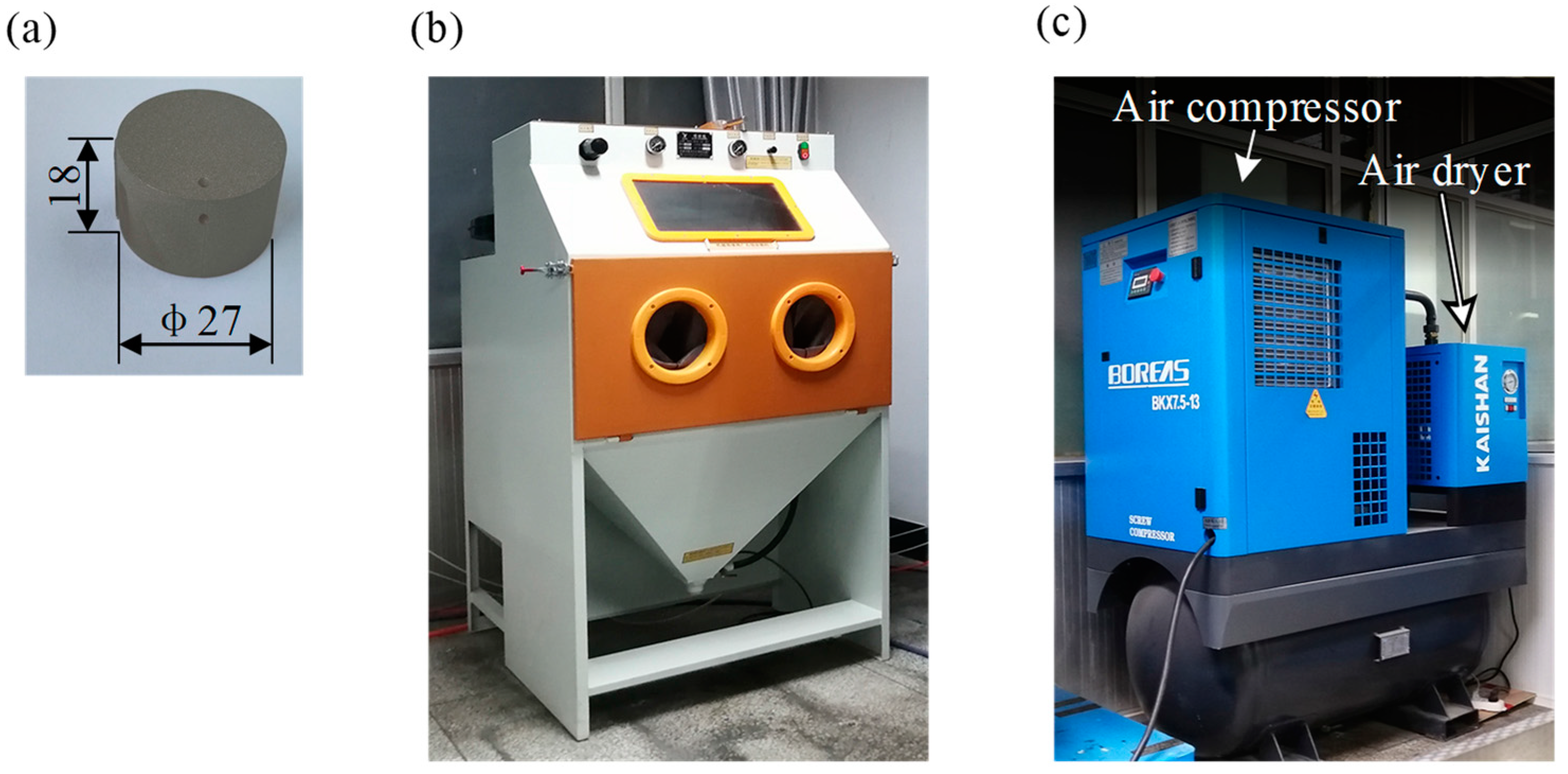
3.1. Preparation of Sandblasted Surface

Figure 4a shows the Inconel 718 samples in the infrared emissivity measurement. The chemical composition and mechanical properties of the material are as reported [39]. The sample is cut from the bulk of the material via electrical discharge wire cutting machining. The heat treatment state of the samples involves solution and aging. The top surface is grinded to eliminate its waviness.
Then, the samples are sandblasted for 15 s at 0.5 Mpa. The blasting angle is 45°. The grit size is selected as 60# alumina ceramic (the diameter is 0.2 mm). Figure 4b,c show the sandblasting device and its air source.

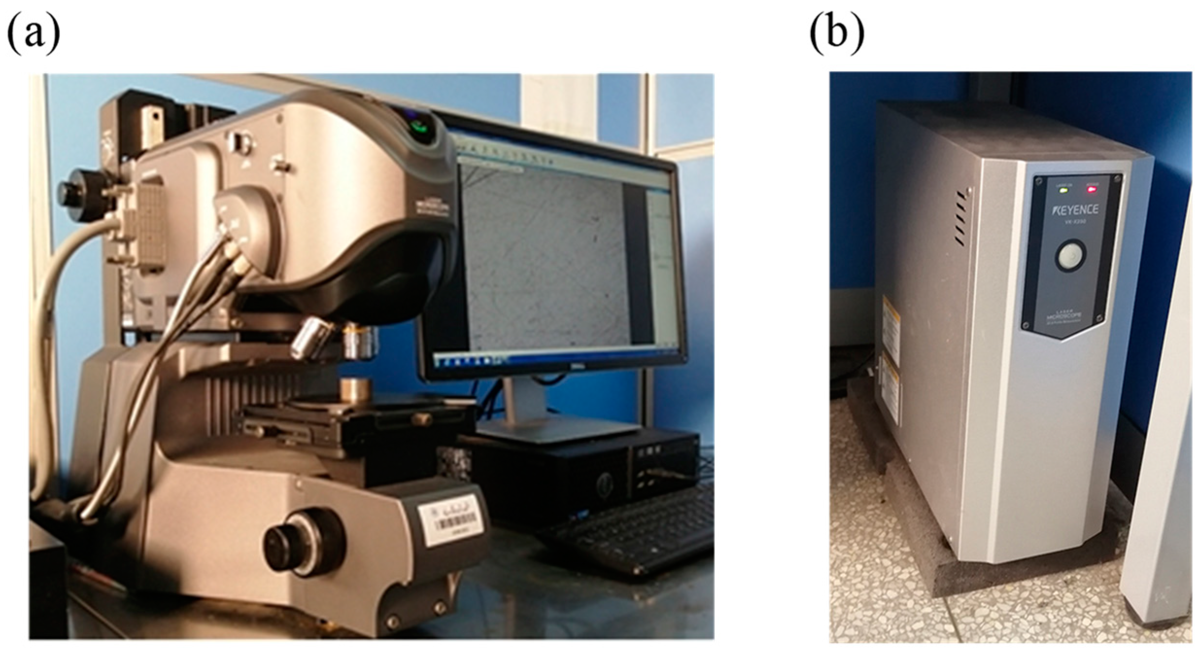
3.2. Surface Morphology Measurement of Sandblasted Samples

The surface morphology of the sandblasted samples is measured using a KEYENCE VK-250 confocal laser scanning microscope (CLSM, Itasca, IL, USA), as shown in Figure 5. The digital signal of the height and slope of the surface element are obtained in the form of a matrix, counted using MATLAB program. In order to remove the high frequency signal cluster from the measured height and slope data, the MATLAB Filter Designer is introduced. The Chebyshev II filter is established. The pass band is set as more than 200 cycles, leading to a wavelength of approximately 0.15. The cutoff band is set as less than 100 cycles, leading to a wavelength of approximately 0.08. The cutoff band amplitude attenuation is 100 dB.

3.3. Directional Spectral Emissivity Measurement of Sandblasted Surface

3.3.1. Method of Directional Spectral Emissivity Measurement

The directional spectral emissivity of a sandblasted surface is measured according to its definition,
ε θ ( λ , T , θ , ϕ ) = E θ ( λ , T , θ , ϕ ) E b ( λ , T )
where  ε θ ( λ , T , θ , ϕ )  is the directional spectral emissivity of the sandblasted surface.  E θ ( λ , T , θ , ϕ )  is the emittance power of the sample.  E b ( λ , T )  is the emittance power of black body.  E θ ( λ , T , θ , ϕ )  and  E b ( λ , T )  are measured using the same equipment. Thus, the error of the emittance power measurement is compensated by the division of  E θ ( λ , T , θ , ϕ )  and  E b ( λ , T ) .
The sample is heated during the directional spectral emissivity measurement. As shown in Planck’s black body radiation law,
E b ( λ , T ) = C 1 λ 5 e C 2 λ T 1
where  λ  is the frequency of the infrared ray, and  T  is the temperature of the sample;  C 1 = 2 π h c 2 3.7418 × 10 16 W m 2  and  C 2 = h c / k 1.4388 × 10 2 m K . The emittance power increases with increasing temperature. The error from the environment is diluted by increased emittance power signal in heating the sample.
The directional spectral emissivity should be measured under the protection of a noble gas environment to prevent oxidation.

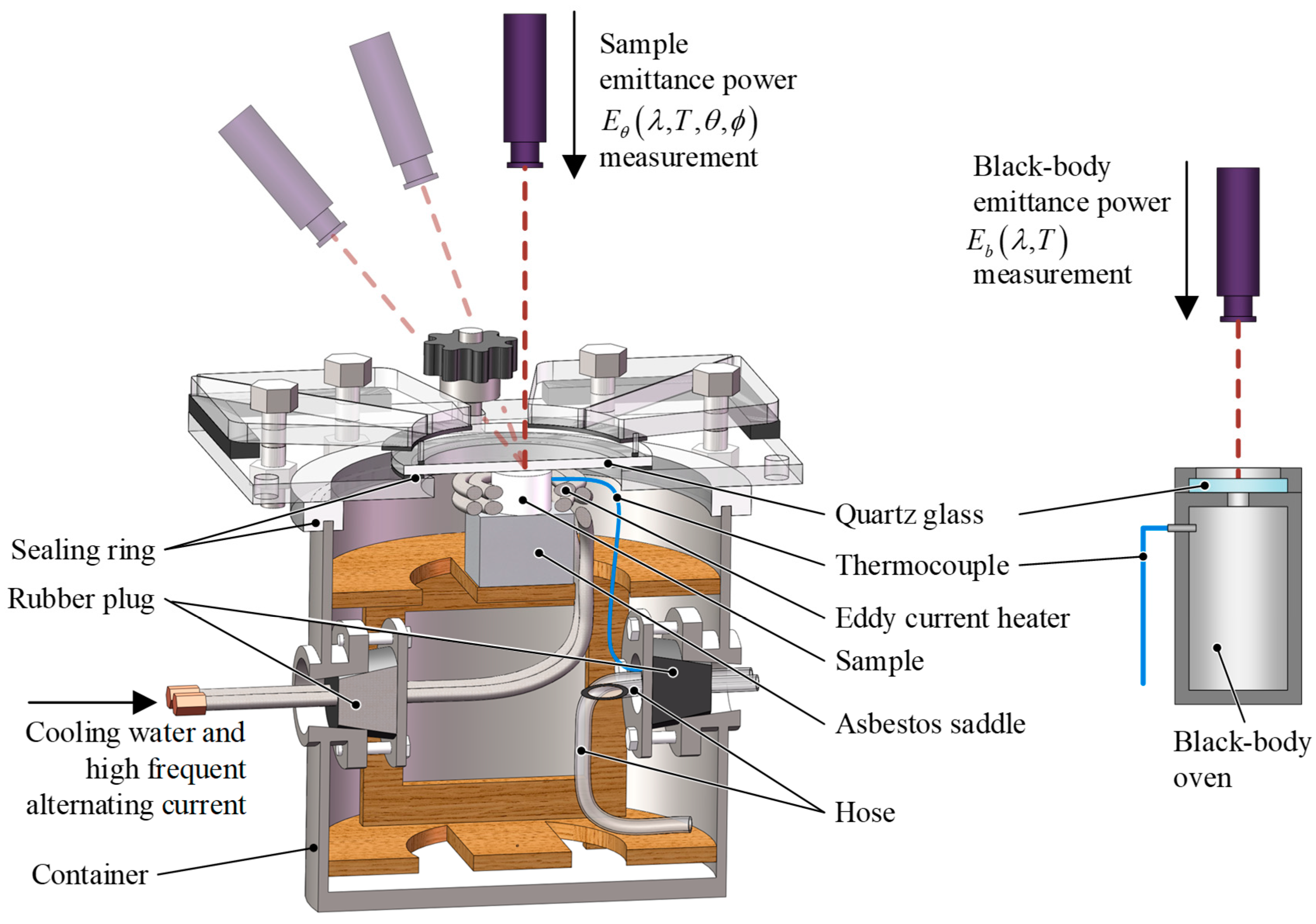
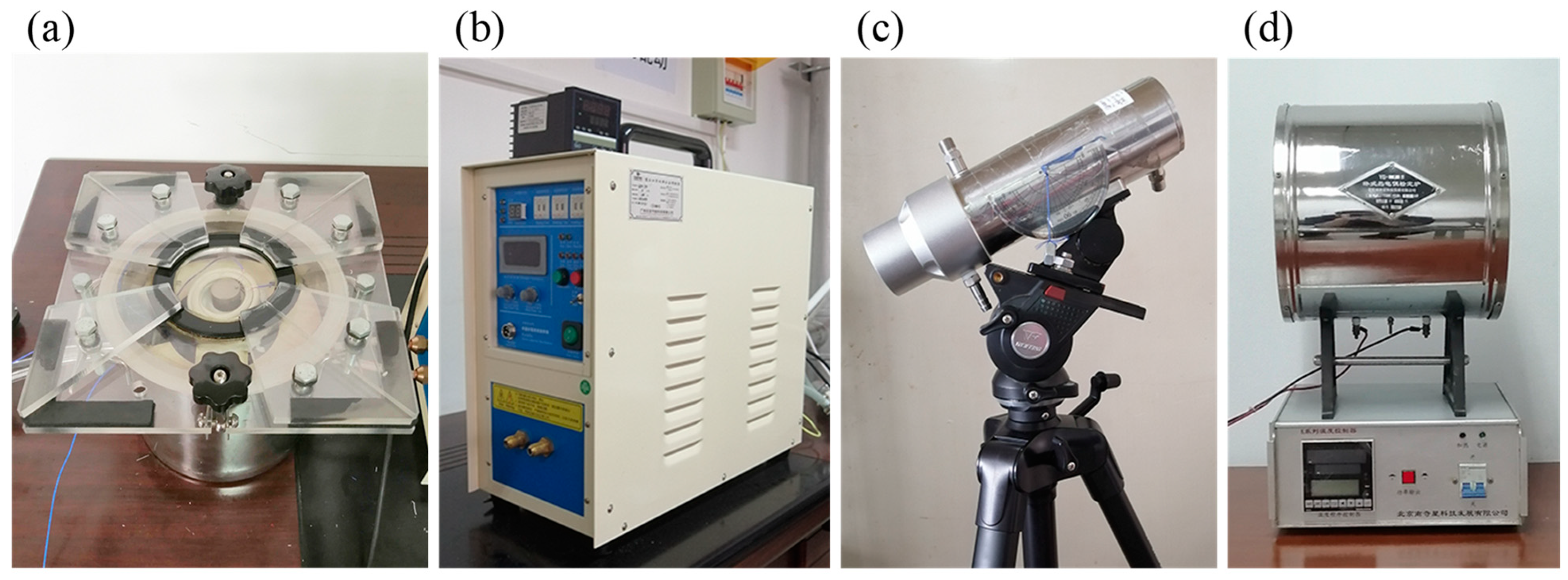
3.3.2. Development of the Directional Spectral Emissivity Measurement Device

The directional spectral emissivity measurement device is developed. Figure 6 shows its 3D digital model. Sealing rings and rubber plugs are used to close the container. Helium is pumped in through the hose to provide a noble gas environment protection. The sample is eddy current heated using the induction coil. The emittance power of the sample  E θ ( λ , T , θ , ϕ )  is measured through the quartz glass.

3.3.3. Procedure of Directional Spectral Emissivity Measurement

The directional spectral emissivity is measured at 773 K in order to decrease the error from environment. Helium is pumped into the container to prevent oxidation. Sample emittance power  E θ ( λ , T , θ , ϕ )  and black-body emittance power  E b ( λ , T )  are measured. Figure 7 shows the directional spectral emissivity measurement equipment. The wavelength of the infrared radiometer is 1.7 μm.

3.4. Infrared Temperature Measurement of Sandblasted Surface

The temperature is measured based on the measured directional spectral emissivity. The emittance power of the sample  E θ ( λ , T , θ , ϕ )  at  T = 773 K  is calculated based on measured emissivity according to
E θ ( λ , T , θ , ϕ ) = ε θ ( λ , T , θ , ϕ ) C 1 λ 5 e C 2 λ T 1
This can be derived using Equations (15) and (16). The directional spectral emissivity is predicted with a Gaussian surface, C-M surface, and Polynomial surface, respectively. The results of the infrared temperature measurement are obtained accordingly.
In introducing the indirect infrared temperature measurement, the errors from other factors including environment and experimental device are excluded, to emphasize the error from directional spectral emissivity prediction.

4. Results and Discussion

4.1. Roughness of Sandblasted Surface

Table 1 shows the surface morphology parameters of the sandblasted surfaces. The arithmetic mean height Sa, the root mean square height Sq, and the root mean square gradient Sdq are relatively high, indicating that the sandblasted surfaces are rough in the sense of both height and slope. The definition of the arithmetic mean height Sa is
S a = 1 A A | Z ( x , y ) | d x d y
where A is the area of the sampling area of the measured surface and Z(x,y) is the height of the surface elements in the sampling area, considered as a function of x and y. The arithmetic mean height Sa shows the volume of the height of the surface are. The definition of the root mean square height Sq is
S q = [ 1 A A Z 2 ( x , y ) d x d y ] 1 2
The root mean square height Sq is the root mean square of the surface height. The root mean square height Sq shows how separated the height of the surface is. The definition of the root mean square gradient Sdq is
S d q = { 1 A A [ Z 2 ( x , y ) x 2 + Z 2 ( x , y ) y 2 ] d x d y } 1 2
where the root mean square gradient Sdq is the root mean square of the slope of all points in the sampling area on the surface. The Sdq shows how separated the slope of the surface is and is regarded by some researchers [39] as the surface morphology parameter most highly related to the directional spectral emissivity of the rough surface. The results shows that the sandblasted surfaces are rough in the sense of both height and slope. The height and slope are widely separated and could not be ignored. The arithmetic mean height Sa and the root mean square height Sq are higher than the wavelength of the infrared radiometer, which is 1.7 μm, meaning that the surface should be considered rough for the given infrared beam. The geometrical optics method adopted in this work is thus verified [30].
The skewness Ssk is close to zero, which shows that the form of the height and slope distribution functions are close to even. The definition of the skewness Ssk is
S s k = 1 S q 3 × A A Z 3 ( x , y ) d x d y
The skewness Ssk is the degree to which the surface height deviates from the average value. The skewness Ssk is close to zero, thus the form of the height and slope distribution functions are assumed even.
The kurtosis Sku > 3, illustrating that the slope is intensively distributed near p = 0. The definition of the kurtosis Sku is
S k u = 1 S q 4 × A A Z 4 ( x , y ) d x d y
where the skewness Sku is the degree to which the surface slope deviates from the average value. If the distribution of the surface slope is Gaussian, the skewness Sku = 3. The higher the skewness Sku is, the tighter the distribution of the surface slope is, and vice versa. The kurtosis Sku > 3, illustrating that the slope is intensively distributed near  p = 0 .
The standard deviation of all parameters is relatively slow compared to the parameters. The surface morphology of the samples shows good consistency and meets the assumed characteristics of an isotropic rough surface. The difference between the samples could be neglected.

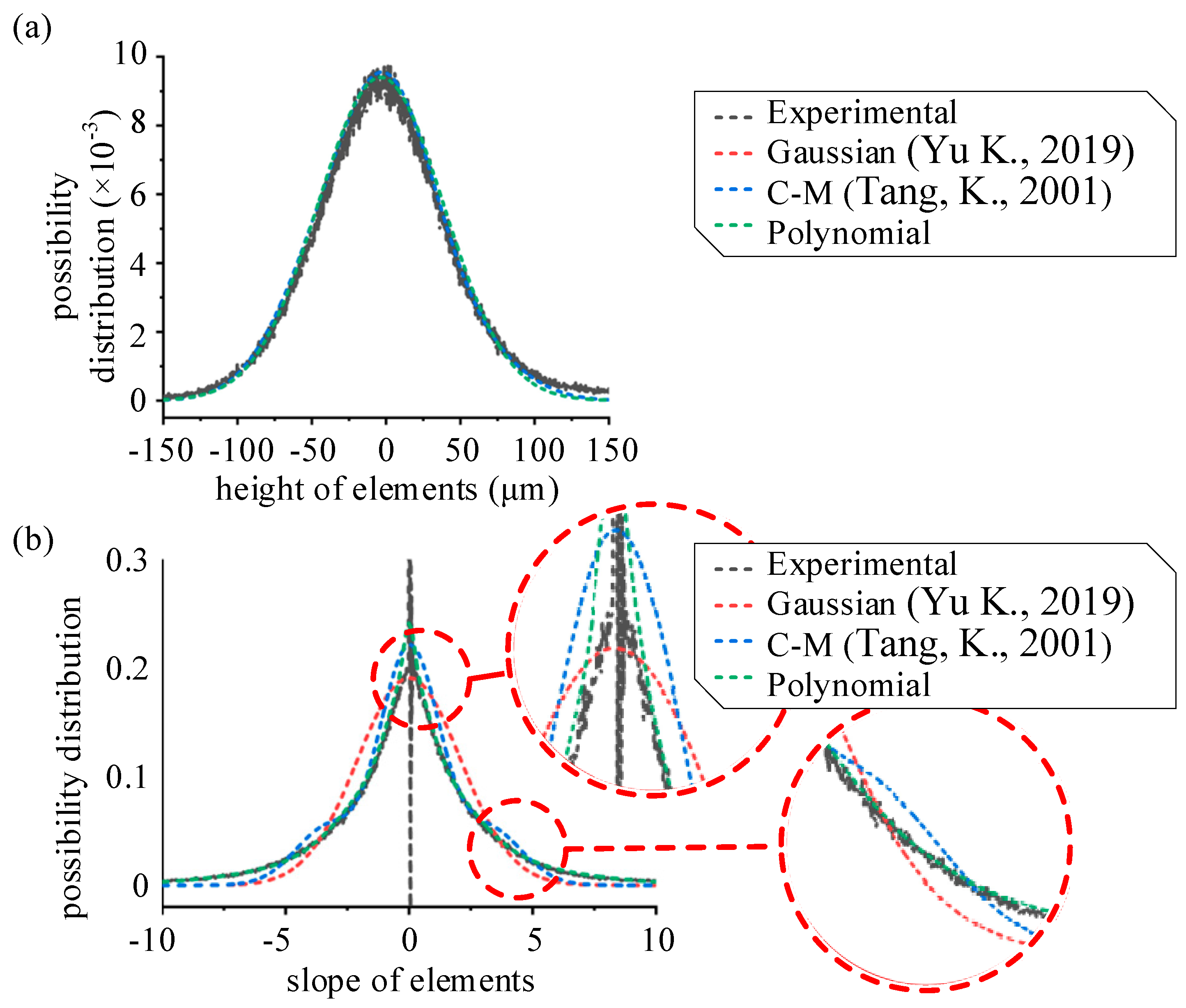
4.2. Surface Morphology Description of Sandblasted Surface

As mentioned before, the form of the slope and height possibility distribution is even. Thus, the Polynomial of Gaussian functions (Polynomial surface) is proposed. The height and slope possibility function of the Polynomial surface is drawn by fitting the experimental data using the MATLAB fitting tool. The kurtosis Sku of the rough metal surface is 6.778, far above 3, showing that the distribution of the slope possibility function is not Gaussian. Thus, a Polynomial of Gaussian functions is needed to accurately describe the function. The slope possibility function of the Polynomial surface is as follows:
f P ( p ) = f P 1 ( p ) + f P 2 ( p )
f P 1 ( p ) = 1 2 π [ b 1 σ P 1 exp ( h 2 2 σ P 1 2 ) + b 2 σ P 2 exp ( h 2 2 σ P 2 2 ) + b 3 σ P 3 exp ( h 2 2 σ P 3 2 ) ]
f P 2 ( p ) = b 4 2 π σ P 4 exp ( h 2 2 σ P 4 2 )
where  f P ( p )  is the slope possibility density function of the Polynomial surface and  f P 1 ( p )  and  f P 2 ( p )  are its components.  f P 1 ( p )  is a Polynomial of Gaussian functions obtained via curve fitting in  p ( 10 , 0.2 ) ( 0.2 , 10 ) , expressing the overall characteristics of the slope possibility distribution.  f P 2 ( p )  is an impulse function representing the peak near p = 0. The parameters are  b 1 = 0.4736 b 2 = 0.3702 b 3 = 0.1356 σ P 1 = 2.056 σ P 2 = 4.658 σ P 3 = 0.7220 σ P 4 = 0.2 , and  b 4 = 0.0217 . The height possibility function of the Polynomial surface is curve fitted as
g P ( h ) = 1 2 π σ P 5 exp ( h 2 2 σ P 5 2 )
where  f P ( p )  is the slope possibility density function of the Polynomial surface.  σ P 5 = 42.33  is the standard deviation of  f P ( p ) .
Figure 8 shows that the proposed Polynomial surface describes the surface morphology more accurate than the Gaussian surface [23,34] and C-M surface [15,35]. The Gaussian surface could not reflect the relatively high kurtosis Sku of the sandblasted surface. The Gaussian surface model assumes that both the height and slope possibility function of the surface are Gaussian, which are not accurate enough. As for the C-M surface, the kurtosis Sku is considered, but error still exists. The reason is that the C-M surface is merely one possible root for a surface with a certain root mean square gradient Sdq, skewness Ssk, and kurtosis Sku, while there is an infinite solution set for such an answer. Thus, the C-M surface is unable to depict the real rough surface accurately. The Polynomial surface depicts the height and slope possibility distribution with relatively high accuracy. To better depict the surface morphology of the rough surface, the impulse function is introduced by setting a relatively low  σ P 4  of the function  f P 2 ( p ) .
To further clarify the cited models, the isotropy Gaussian rough surface is defined as [20,38]
f G ( p ) = 1 2 π σ G 1 exp ( p 2 2 σ G 1 2 )
g G ( h ) = 1 2 π σ G 2 exp ( h 2 2 σ G 2 2 )
where  f G ( p )  and  g G ( h )  are the slope and height possibility density functions of the Gaussian surface, respectively.  σ G 1  and σG2 are the standard deviations of  f G ( p )  and  g G ( h ) . For an isotropy Gaussian surface,  σ G 1 = σ G 2 . For an isotropic rough surface, the C-M surface can be sketched as Equations (32) and (33) [21,33],
f C ( p ) = exp ( p 2 2 σ 2 C 1 ) ( a 1 + a 2 p + a 3 p 2 + a 4 p 3 + a 5 p 4 )
g C ( h ) = exp ( h 2 2 σ 2 C 2 ) ( a 6 + a 7 h + a 8 h 2 + a 9 h 3 + a 10 h 4 )
where  f C ( p )  and  g C ( h )  are the slope and height possibility density functions of the C-M surface, respectively.  σ C 1  and  σ C 2  are the standard deviations of  f C ( p )  and  g C ( h ) a n  are constants.

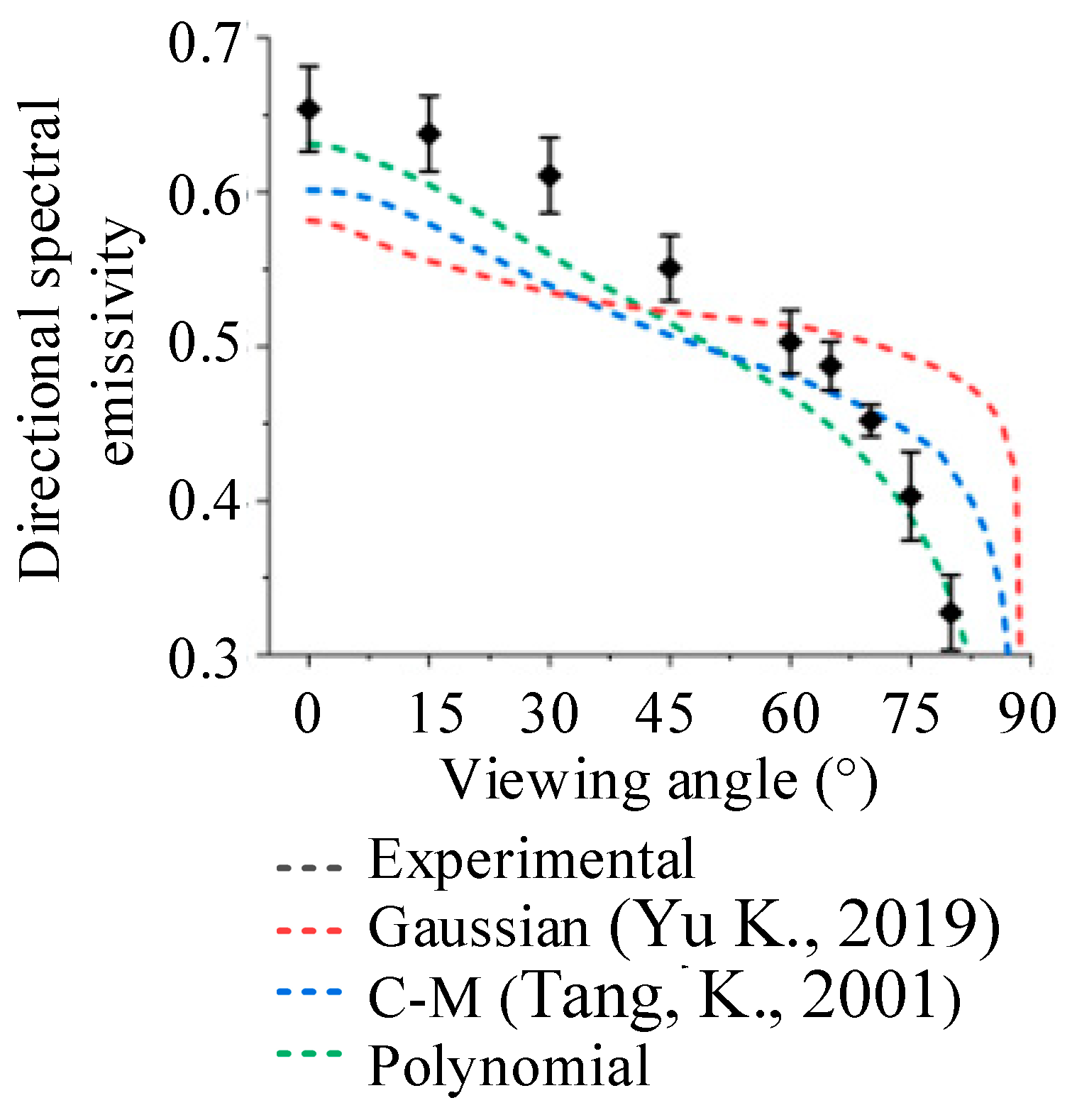
4.3. Comparation of Predicted with Measured Directional Spectral Emissivity

The refractive index n of the material is calculated as 4.26 by substituting the experimental results of Kong et al. [40] into Equation (9). The definition of the domain of height h is defined as  ± 3 σ G 2  ( h [ 127 , 127 ] ) to cover 99% of the elements on the sandblasted surface. The slope q is confined as  q [ 8.457 , 8.457 ] , similarly.
The descripted surface morphology is applied to the isotropic rough surface directional spectral emissivity model. Figure 9 shows the measured and predicted directional spectral emissivity of the sandblasted surface. The directional spectral emissivity of the sandblasted surface decreases with increasing viewing angle. The trend predicted by the Polynomial surface is close to the experimental results, while the Gaussian surface and the C-M surface show more error. The reason is that the Polynomial surface depicts the surface morphology with better accuracy. As mentioned before, the Gaussian surface assumes that both the height and slope possibility function of the surface are Gaussian, and the C-M surface is one possible root for a surface with certain Sdq, Ssk, and Sku. Thus, the surfaces depicted by the Gaussian surface and the C-M surface are less rough compared to the real sandblasted Inconel 718 surface. As we mentioned in our previous work [34], a smooth surface tends to have a peak in a high viewing angle, while the rough surface tends to have a peak in a low viewing angle, leading to an overestimate in a high viewing angle and an underestimate in a low viewing angle.

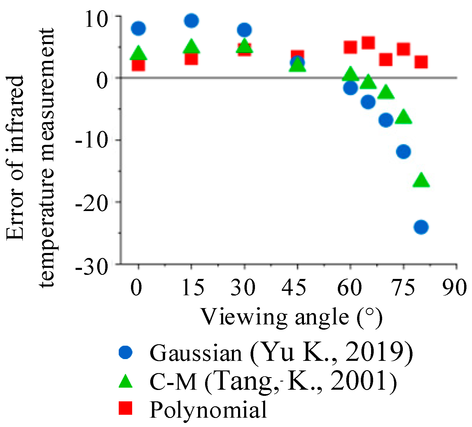
4.4. Accuracy Analysis of Infrared Temperature Measurement

The error of an infrared temperature measurement at 773 K based on a Gaussian surface and C-M surface decreases with the increase in viewing angle. The reason is that the error of directional spectral emissivity with a Gaussian surface and C-M surface decreases with the increase in viewing angle.
Figure 10 shows the error of an infrared temperature measurement of the sandblasted surface. The measured temperature using different emissivity parameters is compared to the results of the thermocouple. The error of infrared temperature measurement at 773 K based on a Gaussian surface fluctuates around 4 K, less than a Gaussian surface and C-M surface. The reason is that a Polynomial surface gives a more precise prediction of the directional spectral emissivity. For a certain signal, an overestimated emissivity leads to an underestimated temperature, and vice versa. Thus, the error of an infrared temperature measurement follows the same pattern of the error of emissivity. The Polynomial surface depicts the morphology of the sample with better accuracy, leading to less and more stable errors. In some cases, the error of temperature measurement could be reduced to 20% (80 degrees, compared to a Gaussian surface). The error of the Polynomial surface could be attributed to the neglected higher-order components in the model or the error of reflectivity n.

5. Conclusions

In this research, a method of prediction of an isotropic rough surface directional spectral emissivity is given. The height and slope possibility density functions are introduced as variables to include the surface morphology. By doing so, more information of the real surface morphology is given to reach a better accuracy. The directional spectral emissivity of the isotropic rough surface is modelled accordingly. Then, as an example and experimental verification, the surface morphology of the sandblasted surfaces is measured, and the Polynomial surface is brought up for description. The directional spectral emissivity measurement and infrared temperature measurement are conducted to verify the model. The main conclusions drawn in this work are as follows:
(1)
The predicted directional spectral emissivity and measured temperature with the surface-morphology-dependent isotropic rough surface directional spectral emissivity model reached a relatively high accuracy, if the surface morphology is properly modelled;
(2)
The sandblasted surface is rough in both the sense of height and slope, and the surface kurtosis  S k u  is large. The surface morphology of the samples shows good consistency and meets the assumed characteristics of isotropic rough surface;
(3)
The Gaussian surface and C-M surface are unable to depict the sandblasted surface morphology accurately, as more assumptions are employed in these models. The Polynomial surface expresses the surface morphology with relatively high accuracy by introducing the distribution of height and slope;
(4)
The directional spectral emissivity of the sandblasted surface decreases with increasing viewing angle, and its slope increases with increasing viewing angle. The Gaussian surface and the C-M surface underestimate the roughness of the surface, introducing more errors in the predicted directional spectral emissivity and measured temperature. The Polynomial surface depicts the surface with better accuracy, leading to a higher accuracy.
For further research, the authors propose the potential translucent layer of collent (in machining) or ocxides (in remote sensing) to be considered in the model.

Author Contributions

Methodology, J.H.; Validation, J.Z.; Formal analysis, Z.L.; Investigation, J.H.; Writing—original draft, J.Z.; Writing—review & editing, Z.L.; Visualization, B.W.; Supervision, B.W. All authors have read and agreed to the published version of the manuscript.

Funding

This research was funded by the National Natural Science Foundation of China grant number No.52275444 and No. 52205482, the Shandong Provincial Key Research and Development Program (Major Scientific and Technological Innovation Project) grant number No.2020CXGC010204, the Postdoctoral Research Foundation of China grant number 2022M711904, the Natural Science Foundation of Shandong Province grant number ZR2022QE011, and the Taishan Scholar Foundation.

Data Availability Statement

The data presented in this study are available on request from the corresponding author.

Conflicts of Interest

The authors declare no conflict of interest.

References

  1. Avanzini, A.; Battini, D.; Gelfi, M.; Girelli, L.; Petrogalli, C.; Pola, A.; Tocci, M. Investigation on fatigue strength of sand-blasted DMLS-AlSi10Mg alloy. Procedia Struct. Integr. 2019, 18, 119–128. [Google Scholar] [CrossRef]
  2. Ahmadi, S.M.; Kumar, R.; Borisov, E.V.; Petrov, R.; Leeflang, S.; Li, Y.; Tümer, N.; Huizenga, R.; Ayas, C.; Zadpoor, A.A.; et al. From microstructural design to surface engineering: A tailored approach for improving fatigue life of additively manufactured meta-biomaterials. Acta Biomater. 2019, 83, 153–166. [Google Scholar] [CrossRef]
  3. Feng, Z.Q.; Wang, L.; Wang, W.Z.; Di Cheng, K.; Chen, C.Z. Failure Analysis of the outside Coating on the Furnace Roller. Appl. Mech. Mater. 2016, 853, 431–435. [Google Scholar]
  4. Guimarães, B.; Rosas, J.; Fernandes, C.M.; Figueiredo, D.; Lopes, H.; Paiva, O.C.; Silva, F.S.; Miranda, G. Real-Time Cutting Temperature Measurement in Turning of AISI 1045 Steel through an Embedded Thermocouple—A Comparative Study with Infrared Thermography. J. Manuf. Mater. Process. 2023, 7, 50. [Google Scholar] [CrossRef]
  5. Heigel, J.; Whitenton, E.; Lane, B.; Donmez, M.; Madhavan, V.; Moscoso-Kingsley, W. Infrared measurement of the temperature at the tool–chip interface while machining Ti–6Al–4V. J. Mater. Process. Technol. 2017, 243, 123–130. [Google Scholar] [CrossRef]
  6. Meola, C.; Boccardi, S.; Carlomagno, G.; Boffa, N.; Ricci, F.; Simeoli, G.; Russo, P. Impact damaging of composites through online monitoring and non-destructive evaluation with infrared thermography. NDT E Int. 2017, 85, 34–42. [Google Scholar] [CrossRef]
  7. DeShong, E.; Peters, B.; Paynabar, K.; Gebraeel, N.; Thole, K.A.; Berdanier, R.A. Applying Infrared Thermography as a Method for Online Monitoring of Turbine Blade Coolant Flow. J. Turbomach. 2022, 144, 1–10. [Google Scholar] [CrossRef]
  8. Xu, D.; Ding, L.; Liu, Y.; Zhou, J.; Liao, Z. Investigation of the Influence of Tool Rake Angles on Machining of Inconel 718. J. Manuf. Mater. Process 2021, 5, 100. [Google Scholar] [CrossRef]
  9. Liu, D.; Liu, Z.; Zhao, J.; Song, Q.; Ren, X.; Ma, H. Tool wear monitoring through online measured cutting force and cutting temperature during face milling Inconel 718. Int. J. Adv. Manuf. Technol. 2022, 122, 729–740. [Google Scholar] [CrossRef]
  10. Peroni, L.; Scapin, M. Plastic Behavior of Laser-Deposited Inconel 718 Superalloy at High Strain Rate and Temperature. Appl. Sci. 2021, 11, 7765. [Google Scholar] [CrossRef]
  11. Liu, Z.; Li, T.; Ning, F.; Cong, W.; Kim, H.; Jiang, Q.; Zhang, H. Effects of deposition variables on molten pool temperature during laser engineered net shaping of Inconel 718 superalloy. Int. J. Adv. Manuf. Technol. 2019, 102, 969–976. [Google Scholar] [CrossRef]
  12. Xu, L.; Chai, Z.; Chen, H.; Zhang, X.; Xie, J.; Chen, X. Tailoring Laves phase and mechanical properties of directed energy deposited Inconel 718 thin-wall via a gradient laser power method. Mater. Sci. Eng. A 2021, 824, 141822. [Google Scholar] [CrossRef]
  13. El Bakali, A.; Gilblas, R.; Pottier, T.; Lieurey, A.; Le Maoult, Y. Effect of oxidation on spectral and integrated emissivity of Ti-6Al-4V alloy at high temperatures. J. Alloy. Compd. 2021, 889, 161545. [Google Scholar] [CrossRef]
  14. Qi, J.; Eri, Q.; Kong, B.; Zhang, Y. The radiative characteristics of inconel 718 superalloy after thermal oxidation. J. Alloy. Compd. 2020, 854, 156414. [Google Scholar] [CrossRef]
  15. Yu, K.; Zhang, H.; Liu, Y.; Liu, Y. Study of normal spectral emissivity of copper during thermal oxidation at different temperatures and heating times. Int. J. Heat Mass Transf. 2019, 129, 1066–1074. [Google Scholar] [CrossRef]
  16. Keller, B.P.; Nelson, S.E.; Walton, K.; Ghosh, T.K.; Tompson, R.V.; Loyalka, S.K. Total hemispherical emissivity of Inconel 718. Nucl. Eng. Des. 2015, 287, 11–18. [Google Scholar] [CrossRef]
  17. Balat-Pichelin, M.; Sans, J.; Bêche, E.; Flaud, V.; Annaloro, J. Oxidation and emissivity of Inconel 718 alloy as potential space debris during its atmospheric entry. Mater. Charact. 2017, 127, 379–390. [Google Scholar] [CrossRef]
  18. Tang, K.; Buckius, R.O. A statistical model of wave scattering from random rough surfaces. Int. J. Heat Mass Transf. 2001, 44, 4059–4073. [Google Scholar] [CrossRef]
  19. Rozanski, L.; Majchrowski, R.; Staniek, R. Choosing of roughness parameters to describe the diffuse reflective and emissive properties of selected dielectrics. Quant. Infrared Thermogr. J. 2014. [Google Scholar] [CrossRef]
  20. Smith, B.G. Geometrical Shadowing of a Random Rough Surface. IEEE Trans. Antennas Propag. 1967, 15, 668–671. [Google Scholar] [CrossRef]
  21. Bourlier, C. Unpolarized infrared emissivity with shadow from anisotropic rough sea surfaces with non-Gaussian statistics. Appl. Opt. 2005, 44, 4335–4349. [Google Scholar] [CrossRef] [PubMed]
  22. Chen, M.; Pang, Q.; Wang, J.; Cheng, K. Analysis of 3D microtopography in machined KDP crystal surfaces based on fractal and wavelet methods. Int. J. Mach. Tools Manuf. 2008, 48, 905–913. [Google Scholar] [CrossRef]
  23. Bourlier, C.; Berginc, G. Shadowing function with single reflection from anisotropic Gaussian rough surface. Application to Gaussian, Lorentzian and sea correlations. Waves Random Media 2003, 13, 27–58. [Google Scholar] [CrossRef]
  24. King, J.L.; Jo, H.; Loyalka, S.K.; Tompson, R.V.; Sridharan, K. Computation of total hemispherical emissivity from directional spectral models. Int. J. Heat Mass Transf. 2017, 109, 894–906. [Google Scholar] [CrossRef]
  25. Jo, H.; King, J.L.; Blomstrand, K.; Sridharan, K. Spectral emissivity of oxidized and roughened metal surfaces. Int. J. Heat Mass Transf. 2017, 115, 1065–1071. [Google Scholar] [CrossRef]
  26. Li, H.; Pinel, N.; Bourlier, C. A monostatic illumination function with surface reflections from one-dimensional rough surfaces. Waves Random Complex Media 2011, 21, 105–134. [Google Scholar] [CrossRef]
  27. Li, H.; Pinel, N.; Bourlier, C. Polarized infrared reflectivity of one-dimensional Gaussian sea surfaces with surface reflections. Appl. Opt. 2013, 52, 6100–6111. [Google Scholar] [CrossRef]
  28. Li, H.; Pinel, N.; Bourlier, C. Polarized infrared reflectivity of 2D sea surfaces with two surface reflections. Remote Sens. Environ. 2014, 147, 145–155. [Google Scholar] [CrossRef]
  29. Li, H.; Pinel, N.; Bourlier, C. Polarized infrared emissivity of 2D sea surfaces with one surface reflection. Remote Sens. Environ. 2012, 124, 299–309. [Google Scholar] [CrossRef]
  30. Wen, C.-D.; Mudawar, I. Modeling the effects of surface roughness on the emissivity of aluminum alloys. Int. J. Heat Mass Transf. 2006, 49, 4279–4289. [Google Scholar] [CrossRef]
  31. Rubanenko, L.; Schorghofer, N.; Greenhagen, B.T.; Paige, D.A. Equilibrium Temperatures and Directional Emissivity of Sunlit Airless Surfaces With Applications to the Moon. J. Geophys. Res. Planets 2020, 125, e2020JE006377. [Google Scholar] [CrossRef]
  32. Warren, T.J.; Bowles, N.E.; Hanna, K.D.; Bandfield, J.L. Modeling the Angular Dependence of Emissivity of Randomly Rough Surfaces. J. Geophys. Res. Planets 2019, 124, 585–601. [Google Scholar] [CrossRef]
  33. Cox, C.; Munk, W. Some problems in optical oceanography. J. Mar. Res. 1995, 14, 63–78. [Google Scholar]
  34. Hu, J.; Liu, Z.; Zhao, J.; Wang, B.; Song, Q. Theoretical Modeling and Analysis of Directional Spectrum Emissivity and Its Pattern for Random Rough Surfaces with a Matrix Method. Symmetry 2021, 13, 1733. [Google Scholar] [CrossRef]
  35. Bourlier, C.; Berginc, G.; Saillard, J. Monostatic and bistatic statistical shadowing functions from a one-dimensional stationary randomly rough surface according to the observation length: I. Single scattering. Waves Random Media 2002, 12, 145–173. [Google Scholar] [CrossRef]
  36. Yoshimori, K.; Itoh, K.; Ichioka, Y. Optical characteristics of a wind-roughened water surface: A two-dimensional theory. Appl. Opt. 1995, 34, 6236–6247. [Google Scholar] [CrossRef]
  37. Smith, B.G. Lunar surface roughness: Shadowing and thermal emission. J. Geophys. Res. 1967, 72, 4059–4067. [Google Scholar] [CrossRef]
  38. Zhao, J.; Liu, Z.; Wang, B.; Hua, Y.; Wang, Q. Cutting temperature measurement using an improved two-color infrared thermometer in turning Inconel 718 with whisker-reinforced ceramic tools. Ceram. Int. 2018, 44, 19002–19007. [Google Scholar] [CrossRef]
  39. Hu, Y.Z.; Tonder, K. Simulation of 3-D random rough surface by 2-D digital filter and fourier analysis. Int. J. Mach. Tools Manuf. 1992, 32, 83–90. [Google Scholar] [CrossRef]
  40. Kong, B.; Li, T.; Eri, Q. Normal spectral emissivity measurement on five aeronautical alloys. J. Alloys Compd. 2017, 703, 125–138. [Google Scholar] [CrossRef]
Figure 1. Framework of the paper. Date from [15,18].
Metals 13 01679 g001
Figure 2. Mechanism of area projection coefficient. (a) Surface element. (b) Projection of the element [34].
Metals 13 01679 g002
Figure 3. Shadow process of infrared electromagnetic wave emitted from rough surface.
Metals 13 01679 g003
Figure 4. Sandblasting experimental set-up. (a) Sample. (b) Sandblasting device. (c) Air source of sandblasting device.
Metals 13 01679 g004
Figure 5. Confocal laser scanning microscope in sandblasted surface morphology measurement. (a) Confocal laser scanning microscope. (b) Controller of the confocal laser scanning microscope.
Metals 13 01679 g005
Figure 6. Directional spectral emissivity measurement device.
Metals 13 01679 g006
Figure 7. Directional spectral emissivity measurement equipment. (a) Homemade directional spectral emissivity measurement device. (b) High frequent power supply. (c) Infrared radiometer. (d) Black-body furnace.
Metals 13 01679 g007
Figure 8. Surface height and slope possibility density function using Gaussian surface, C-M surface, Polynomial surface, and experimental results. (a) Height possibility density function. (b) Slope possibility density function. Date from [15,18].
Metals 13 01679 g008
Figure 9. Measured and predicted directional spectral emissivity of sandblasted surface. Date from [15,18].
Metals 13 01679 g009
Figure 10. Infrared temperature measurement simulation of the sandblasted surface. Date from [15,18].
Metals 13 01679 g010
Table 1. Surface morphology parameters of sandblasted samples.
ParameterSa (μm)Sq (μm)SdqSskSku
mean3.7695.2655.2840.6666.778
standard deviation0.0520.0830.2070.0960.180
Disclaimer/Publisher’s Note: The statements, opinions and data contained in all publications are solely those of the individual author(s) and contributor(s) and not of MDPI and/or the editor(s). MDPI and/or the editor(s) disclaim responsibility for any injury to people or property resulting from any ideas, methods, instructions or products referred to in the content.

