Abstract
The scope of this work is to present a reverse engineering (RE) methodology to achieve accurate polygon models for 3D printing or additive manufacturing (AM) applications, as well as NURBS (Non-Uniform Rational B-Splines) surfaces for advanced machining processes. The accuracy of the 3D models generated by this RE process depends on the data acquisition system, the scanning conditions and the data processing techniques. To carry out this study, workpieces of different material and geometry were selected, using X-ray computed tomography (XRCT) and a Laser Scanner (LS) as data acquisition systems for scanning purposes. Once this is done, this work focuses on the data processing step in order to assess the accuracy of applying different processing techniques. Special attention is given to the XRCT data processing step. For that reason, the models generated from the LS point clouds processing step were utilized as a reference to perform the deviation analysis. Nonetheless, the proposed methodology could be applied for both data inputs: 2D cross-sectional images and point clouds. Finally, the target outputs of this data processing chain were evaluated due to their own reverse engineering applications, highlighting the promising future of the proposed methodology.
1. Introduction
Reverse Engineering (RE) is defined as the regression of a common forward engineering process. This technique was boosted during the Second World War, and, currently, it is widely implemented in the industrial sector [1,2,3,4] and the medical field [5,6,7], as well as in other areas. This fact is due to its usefulness for getting technical information from a real part by using different data acquisition methods and processing this information in order to achieve the virtual model of the part. Therefore, this process is really valuable not only when there is a lack of technical information about one workpiece, but also when the comparison between the CAD model of the part and the manufactured part provides a high added value for understanding the manufacturing process and trying to improve it.
There are different data acquisition methods, which could be classified based on their system for achieving data. Following this assumption, there are three main methods: the contact, non-contact and destructive methods. The outputs of these methods are frequently 2D cross-sectional images or point clouds, depending on the selected method. 2D cross-sectional images are the general output of destructive methods and some non-contact methods such as Magnetic Resonance Imaging (MRI) or Computed Tomography (CT). Hence, point clouds are the widespread output of almost all other methods. The next step is related to processing this data in order to obtain the 3D model of the part. The final outcomes of this data processing chain could be polygon meshes or NURBS (Non-Uniform Rational B-Splines). Polygon mesh models are commonly in a STL file format, and therefore used for additive manufacturing or 3D printing applications. NURBS surfaces are normally used in CAD-CAM-CAE applications due to their parametrized nature [8].
Therefore, data processing in order to obtain the 3D CAD model of the part based on NURBS surfaces is one of the most interesting challenges of an RE process. This is because polygon models only assure positional continuity (C0), whilst NURBS surfaces also offer tangential (C1) and curvature (C2) continuity [9,10]. In other words, they allow design modifications while polygon models do not. Thus, these models provide a wider range of engineering possibilities e.g., these models are suitable for the recovery of damaged parts, availing of machining, additive manufacturing (AM) and 3D printing techniques [11,12,13,14]. In addition, there is a trend in research activities related to additive technologies towards the use of 4D printing [15].
Nonetheless, the general output of this kind of process is a 3D polygon model. This fact is due to the very nature of the data. Point clouds are defined by the 3D coordinates of each point, while 2D cross-sectional images show the 2D coordinates per slice. Processing these data in order to obtain the 3D polygon models may imply less effort than NURBS surface generation. This makes sense due to the fact that, frequently, NURBS surfaces are constructed using 3D polygon models as a reference. Point clouds or 2D cross-sectional images are also used for this purpose [16]. These elements could be used for creating reference geometries such as points, curves and primitives in order to generate NURBS surfaces. The workflow of the RE data processing chain is shown in Figure 1.
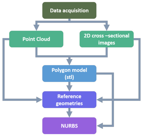
Figure 1.
RE data processing chain.
It is worth mentioning that the accuracy of the 3D models generated by this RE process depends on the data acquisition system, the scanning conditions and the data processing techniques [17]. As stated above, the output of this data processing chain could be used as input for additive manufacturing or advanced machining processes. The manufacturing process selected to complete the RE chain, as well as the manufacturing parameters of the process, have their own influence on the dimensional accuracy and the deviation of the resulting workpiece [18,19]. Nonetheless, these effects are not analyzed in this paper.
This work is focused on the data processing step in order to assess the accuracy of applying different processing techniques. Moreover, the proposed methodology could be applied for both data inputs: 2D cross-sectional images and point clouds. Finally, the target outputs of this data processing chain would be evaluated due to their own reverse engineering applications.
2. Materials and Methods
According to the previous statement, this work is focused on the data processing step for achieving polygon models and NURBS surfaces of scanned workpieces by means of different data acquisition systems. To this end, four industrial workpieces were selected, with the aim of investigating the effect of different materials and geometries on the outcomes. The characteristics of each one are detailed in Table 1. In Figure 2, all of them are presented.

Table 1.
Workpieces and materials for case studies.
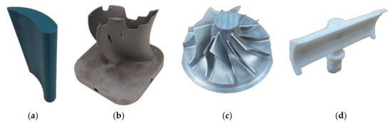
Figure 2.
Workpieces of case studies: (a) CS-1; (b) CS-2; (c) CS-3; and (d) CS-4.
2.1. Data Aquisition
For this study, both, X-ray computed tomography (XRCT) and a Laser Scanner (LS) were selected. Nonetheless, the methodology proposed below could be applied to any other data acquisition method.
On the one hand, a General Electric X-Ray machine model X-Cube Compact (Baker Hughes, Houston, TX, USA) with five axes was used for scanning purposes. The maximum voltage and current of the XRCT system are 195 kV and 8 mA, respectively, and the small/large focus sizes are 0.4/1 mm. The scanning conditions by XRCT for each case study are summarized in Table 2. The selection of the scanning conditions depends on the workpiece dimensions and material. This is due to the fact that the transmission of X-rays through the material is determined by the attenuation coefficient, which is related to the thickness to be scanned, the material density and the atomic number of the material. In order to achieve quality projections for XRCT reconstruction, the X-rays should be able to penetrate the workpiece with sufficient contrast. Hence, the scanning conditions for each case study were established according to the previous statement. Owing to the fact that CS-2 and CS-3 are metal workpieces with larger dimensions than CS-1 and CS-4, which are plastic workpieces, the scanning conditions selected to assure the X-ray penetration are higher in those cases. Finally, the software VGStudio MAX2.2 (Volume Graphics, Heidelberg, Germany) was used for XRCT reconstruction.
Table 2.
Scanning conditions by XRCT for each case study.
On the other hand, these workpieces were also digitalized through a coordinate measuring machine (CMM) model Crysta Apex S 9106, equipped with a non-contact line-laser probe (LS) model SurfaceMeasure 606T (Mitutoyo, Takatsu-ku, Kawasaki-shi, Japan). The resolution of the CMM system is 0.0001 mm. The maximum acquisition rate of the LS system is 3 × 25,500 points/s, with 0.017 mm of scanning error (according to Mitutoyo’s acceptance procedure). As illustrated in Figure 3, the scanning procedure was set for all case studies, taking 17 positions of the LS. Once these scans from different positions were obtained, they were automatically combined into one single point cloud by the software MSURF V5.0 (manufactured by MitutoyoCo. Ltd., Takatsu-ku, Kawasaki-shi, Japan). The number of vertices of these point clouds is summarized in Table 3.
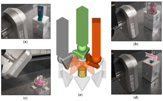
Figure 3.
The LS scanning procedure for all case studies: (a) CS-1; (b) CS-2; (c) CS-3; (d) CS-4; and (e) the 17 LS scanning positions: one for every 45 degrees at both, 90 degrees (grey) and 45 degrees (orange) of the LS, and only one at 0 degrees of the LS (green).
Table 3.
Number of vertices in the point cloud for each case study.
2.2. Data Processing
Once the outputs of the previous step were obtained, they were analyzed for the application of different processing techniques in order to achieve accurate 3D models of the scanned workpieces. Therefore, the main aim of this section is to assess the influence of the implementation of different data processing techniques, as well as to propose a methodology for carrying out this complicated task. To address this issue, the following steps of the data processing chain were investigated:
- Image processing,
- Point cloud processing,
- Generation of polygon models,
- Reference geometries extraction,
- NURBS surface generation.
Owing to the very nature of the data inputs, both cases were analyzed separately. The methodology proposed by this work consists of processing the input data for achieving polygon models and NURBS surfaces of the scanned workpieces. Special attention is given to the XRCT data processing step, using different approaches to accomplish this task. For that reason, the polygon models generated from the LS point clouds processing step were utilized as a reference to perform the deviation analysis. Finally, the RE methodology proposed by this work is presented in Figure 4.
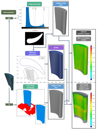
Figure 4.
General scheme of the proposed RE methodology.
To carry out the presented methodology, different software were used. First, the XRCT data were processed by a homemade data processing workflow developed in MATLAB software (MathWorks, Natick, MA, USA). In addition, CATIA V5 (Dassault Systèmes SE, Vélizy-Villacoublay, France) was utilized in the last step. However, for LS data processing, not only MATLAB software was utilized, but also MSURF software. Finally, the deviation analysis was carried out by GOM Inspect 2019 (GOM GmbH, Braunschweig, Germany).
2.2.1. Image Processing
The main purpose of image processing is to obtain information from input images by applying different processing techniques. When dealing with XRCT data, the most common image processing techniques are contrast adjustment, image filtering and image segmentation, amongst others [20]. In this context, image segmentation plays a major role in the process of achieving accurate 3D models of the scanned workpieces. Hence, this section focuses on this topic.
There are different image segmentation techniques. In this case, thresholding-based techniques were analyzed. Thresholding is the simplest image segmentation method. For grayscale images, it consists of checking the value of each pixel intensity and comparing it with the threshold value assigned for the data segmentation. Therefore, the grayscale image could be binarized by following this expression:
where I(i,j) is the intensity value of the pixel located at i row and j column of the image pixel matrix. Additionally, T(i,j) is the threshold value assigned for the data segmentation, which could be the same value for all image pixels if it is global, or different values for each pixel if it is local. BW(i,j) is the binary image output.
The same principle is applied when the data inputs are 3D volumes instead of 2D images. Adding the third dimension of the voxel matrix to the expression:
where k refers to the third dimension of the voxel matrix.
Hence, this segmentation method could be used to differentiate between two parts, the background and foreground. Normally, black pixels are assigned for the background, whereas white pixels indicate the foreground. In addition, assigning multiple threshold values is also possible and useful, especially when there are different materials or components.
Thresholding methods are classified into six different groups according to [21]. For the sake of simplicity, they could be divided into global or local groups based on their threshold value estimation strategy. In terms of computational efficiency, global methods are usually faster than local ones due to their calculations being performed only once. Therefore, employing global methods to determine the threshold value could be well-founded, especially when the appearance of the data histogram is close to bi-modal and when the contrast between the foreground and background is properly defined. For single-material workpieces scanned by means of XRCT, these requirements could be fulfilled. That is how the application of the global methods could be recommended in this case. In order to evaluate their influence on the accuracy of the 3D models generated by the proposed methodology, some of the most straightforward global methods are detailed below.
ISO50
This is a common histogram-shape-based method. It is widely implemented in commercial software packages due to its computational speed and easy comprehension. Its effectiveness depends on the acquired histogram data, e.g., it works really well for bi-modal histograms. This is caused by this method being based on detecting the two main peaks on the histogram and assigning the threshold value at the average intensity value between them. Therefore, the ISO50 threshold T is calculated as:
where Mb is the modal value for the background, whereas Mf is the modal value for the foreground [22].
Valley
The method proposed here is based on the same assumption as the previous one. Nevertheless, in this case, the threshold value is assigned to the minimum value of the histogram between the two main peaks instead of the average value between them. In order to avoid local effects on the results, the histogram is usually normalized and smoothed. Hence, the threshold value is estimated by the following expression:
where h(g) is the histogram of the image, and g is the grey value of the gray scale.
Otsu
The Otsu method is a well-known method for image thresholding due to its effectiveness. Indeed, it is widely implemented and remains one of the most referenced methods. According to [21], it is defined as a Clustering Thresholding method that deals with the variance of the foreground and background pixels in order to minimize this value [23].
2.2.2. Point Cloud Processing
Once the point cloud outputs of the data acquisition step by LS are obtained, data optimization is needed. This processing approach is mainly based on well-known point cloud processing techniques such as merging, reducing redundant vertices, clustering based on Euclidean distance and noise filtering for removing outliers [24]. As a result, the number of points in the point cloud data are minimized so that it is easier to handle for polygonization.
2.2.3. Generation of Polygon Models (STL)
These models are one of the outputs of this data processing approach. They are widely used in 3D printing and additive manufacturing applications. Hence, the developments of data processing techniques in order to achieve more accurate polygon models from raw data are a current challenge.
Regarding polygon model generation from image processing, some isocontouring algorithms have been developed, such as Marching Cubes [25] or Flying Edges [26]. These algorithms allow one to extract a polygonal mesh from a 3D scalar field by approximating the isosurface at a specified isovalue [27]. In this case, the isosurface extraction from the scalar fields generated by the proposed image processing techniques was carried out using the Marching Cubes algorithm. To this end, MATLAB software was used.
Moreover, specially developed software are available for point cloud polygonization. Most of them are based on Delaunay triangulations, due to their favorable geometric properties. These software produce a triangular mesh using the points and the triangulation connectivity list obtained by the polygonization step. For this purpose, the aforementioned software MSURF was used.
2.2.4. Reference Geometries Extraction
As described in Section 1, polygon models, as well as point clouds or 2D cross-sectional images are used as a reference for the 3D CAD modeling. For simple geometries, this task could be accomplished directly by editing or fitting operations. However, complex parts require a different approach. In this context, sectioning and working with curves lead the process [9,10,28].
The sectioning step consists of slicing the model in order to obtain 2D cross-sectional contours of the scanned workpieces. This task is carried out by following different strategies, depending on the input data.
- For polygon models, the intersection with the defined plane is used,
- For point clouds, the nearest points are projected onto the defined plane,
- For 2D cross-sectional images, the images themselves correspond to a section. The reconstruction of the volume from the images is also used to define different planes.
Once this step is concluded, the obtained geometries are approximated by curve-fitting operations [29]. There are different approaches developed for this purpose, such as smoothing splines [30], B-splines [31,32] and Bézier curves, amongst others.
Therefore, the outcomes of this process conduct the NURBS surface generation step, thereby selecting the correct direction and the distance between the slices, and performing an optimal curve fitting approximation implies the success of the proposed procedure.
2.2.5. NURBS Surface Generation
Apart from 3D polygon models, NURBS surfaces are the final output of the presented RE methodology. They are widely used in CAD-CAM-CAE applications owing to the fact that they not only assure positional continuity (C0), but also offer tangential (C1) and curvature (C2) continuity. Hence, 3D CAD models based on NURBS surfaces allow design modifications, which is one of the most interesting challenges of a RE process.
The interest of using NURBS for curves’ and surfaces’ definition is due to the trend of using freeforms in part design and their ability to define these geometries in an accurate way.
As stated above, NURBS surfaces could be constructed by using polygon models for surface fitting or approximated curves as reference geometries. In this case, the second strategy was selected because of the complex geometries of the workpieces. The software CATIA V5 was used for this purpose.
3. Results and Discussion
This section aims to present the results obtained by applying the data processing techniques described in Section 2.2. To this end, the results of each step of the data processing chain were analyzed:
- Image processing,
- Point cloud processing,
- Generation of polygon models (STL),
- Reference geometries extraction,
- NURBS surface generation.
3.1. Image Processing
In order to assess the influence of applying different thresholding-based techniques for the image segmentation, the processing techniques described in Section 2.2.1 were performed on each sample, as shown in Figure 5, Figure 6, Figure 7 and Figure 8. The threshold values estimated by implementing these processing techniques were analyzed, due to the accuracy of the 3D models generated from these methods depending on these calculated values. The higher the threshold value, the lower the volume of the obtained model. To ensure the accuracy of the proposed methodology, 3D scalar fields generated by means of XRCT were processed with the aim of distinguishing the above-defined threshold values. To compute the threshold values of the case studies, MATLAB software was used.
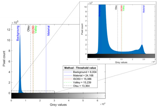
Figure 5.
Histogram of the original greyscale volume from XRCT and threshold values estimated by applying three different thresholding-based techniques for image segmentation on CS-1.
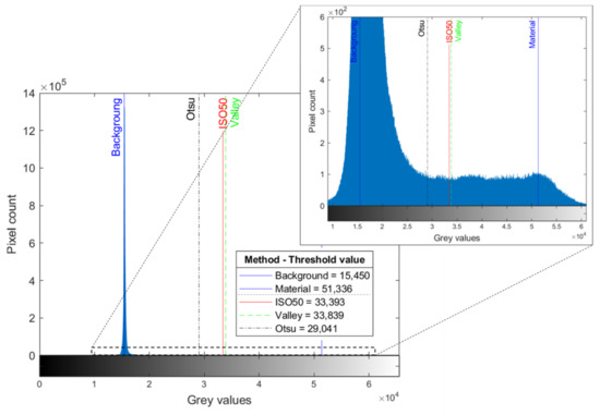
Figure 6.
Histogram of the original greyscale volume from XRCT and threshold values estimated by applying three different thresholding-based techniques for image segmentation on CS-2.
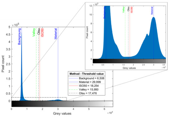
Figure 7.
Histogram of the original greyscale volume from XRCT and threshold values estimated by applying three different thresholding-based techniques for image segmentation on CS-3.
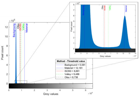
Figure 8.
Histogram of the original greyscale volume from XRCT and threshold values estimated by applying three different thresholding-based techniques for image segmentation on CS-4.
According to the obtained results, for the CS-1 (Figure 5), CS-2 (Figure 6) and CS-4 (Figure 8) cases, the Valley method presents the largest values followed by ISO50 and Otsu. In addition, ISO50 provides a higher value than Otsu for all case studies. Nevertheless, the threshold value determined by the Valley method for CS-3 (Figure 7) is the lowest one.
Additionally, the values obtained by ISO50 and Otsu for CS-3 (Figure 7) and CS-4 (Figure 8) are significantly close. Meanwhile, this effect is not fulfilled for CS-1 (Figure 5) and CS-2 (Figure 6), where the ISO50 threshold value approximates the Valley-estimated value.
Finally, this assessment reveals that the effectiveness of employing these methods for threshold value estimation is strongly dependent on the histogram of the data that is to be processed. This is owing to the fact that ISO50 and Valley are histogram-shape-based methods, which essentially search peaks and valleys. Therefore, using these methods to find the optimal threshold value for image segmentation is well-founded when the histogram is close to a bi-modal distribution. In contrast, the Otsu method is a Clustering Thresholding method, which deals with variances for choosing the optimal threshold. Hence, this method also needs this type of histogram, with equal variances, for a proper estimation [33].
3.2. Point Cloud Processing
Following the procedure stated in Section 2.2.2, the number of points in the point cloud of each case study was reduced, as shown in Table 4 (Section 3.3). Thus, the resulting point clouds were suitable for polygon model generation.
Table 4.
Number of points in the point clouds and polygon models for each case study.
3.3. Generation of Polygon Models (STL)
According to the Section 2.2.3, the polygon model generation follows different approaches depending on the input data. From the XRCT data, the polygon models were generated by the Marching Cubes algorithm, using the threshold values estimated in Section 3.1. To this end, MATLAB software was used. Regarding the polygon model generation from LS point clouds, MSURF software was utilized. The point clouds optimized in Section 3.2 were used for polygonization. The number of points in the point clouds generated by the previous steps are summarized in Table 4, as are the number of points in the meshes obtained by the generation of polygonal models.
GOM Inspect 2019 was used to analyze the deviations between the polygon models generated by the previous steps. In order to assess the accuracy of applying the proposed image processing techniques, comparisons were developed by setting the LS polygon models as a reference. The results are shown in Figure 9, Figure 10, Figure 11 and Figure 12.
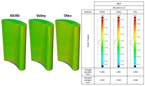
Figure 9.
Comparison of the obtained XRCT surfaces by different thresholding methods with the laser scan as the ground truth for CS-1.
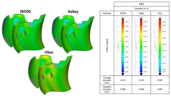
Figure 10.
Comparison of the obtained XRCT surfaces by different thresholding methods with the laser scan as the ground truth for CS-2.
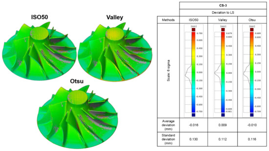
Figure 11.
Comparison of the obtained XRCT surfaces by different thresholding methods with the laser scan as the ground truth for CS-3.
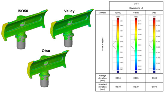
Figure 12.
Comparison of the obtained XRCT surfaces by different thresholding methods with the laser scan as the ground truth for CS-4.
For further discussion, the results obtained by polygon model comparisons are summarized in Figure 13. For clarification, the deviation positive values mean that the polygon models generated by the XRCT data processing step are higher than the polygon model generated by the LS data processing step, while negative values indicate the opposite effect.
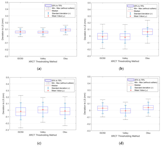
Figure 13.
Summarized results of the comparisons of the XRCT surfaces obtained by different thresholding methods with the laser scan as the ground truth, for each case study: (a) CS-1; (b) CS-2; (c) CS-3; and (d) CS-4.
Figure 13a (CS-1) exhibits that the mean value of the deviation results is nearly the same for ISO50 and Valley. It is increased by around 50% when using the Otsu method, reaching 0.093 mm. Nonetheless, the standard deviation remains constant for all methods, with values close to 0.045 mm. These results suggest that all methods overestimate the volume of the scanned workpiece, though the range of the deviation values is the lowest out of all the case studies.
In Figure 13b (CS-2), the mean values achieved by ISO50 and Valley, which have a distance of 0.006 mm between them, are very close to zero. Furthermore, the standard deviation values obtained by these methods are almost the same. In contrast, Otsu increases the mean value to 0.061 mm while reducing the standard deviation by about 23%, achieving 0.067 mm.
Figure 13c (CS-3) shows that ISO50 increases the mean value and the standard deviation by approximately 60% and 12% of the values obtained by Otsu. Valley presents the lowest values for both, reaching 0.009 mm and 0.112 mm, respectively.
According to Figure 13d (CS-4), Valley achieves the lowest mean value of the deviation results, while ISO50 and Otsu increase this value from 0.005 mm to 0.034 mm and 0.043 mm, respectively. Nevertheless, their standard deviation remains constant.
Even so, all the mean values reached by these methods are below 0.100 mm, with 0.130 mm being the maximum standard deviation value out of all the case studies.
Therefore, the results are consistent with the threshold values estimated in Section 3.1. Similar thresholds present similar results. In this context, the Valley method provides the lowest combination of mean and standard deviation values for CS-1, CS-3 and CS-4. In addition, the results obtained for CS-2 are really close to those obtained by ISO50. Hence, it could be well-founded to apply the Valley method in all case studies due to the obtained results. Nonetheless, this method is strongly dependent on the histogram appearance, so its application might not be suitable in other circumstances.
Regarding the material and geometry effects on the outcomes, it is worth mentioning that they have their own influence apart from other variables. The growth of deviations between models possibly comes from tomography error sources that could be increased due to material and geometry complexities [34]. Therefore, the more complex the material and the geometry of the workpiece were, the more discrepancies were found.
3.4. Reference Geometries Extraction
The methodology proposed here is based on the assumption that the design of the scanned workpieces is built on sweep operations as its base. Therefore, the assessment of the following steps will be carried out only for CS-1 and CS-2, which fulfill this requirement.
According to the previous results, the Valley method was selected to continue the study. The processed 3D scalar fields, which were generated from CS-1 and CS-2 XRCT data, were each sectioned at 5.253 mm and 3.874 mm, respectively. Afterwards, the resulting profile geometries were approximated by curve fitting operations, as shown in Figure 14. To this end, the NURBS toolbox was utilized [35].
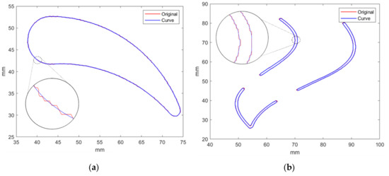
Figure 14.
Comparison between the original profile geometry obtained by XRCT data sectioning (red) and the approximated curve achieved by fitting operations (blue), for each case study: (a) CS-1; (b) CS-2.
3.5. NURBS Surface Generation
As stated above, the NURBS surface generation was carried out using the approximated curves created by the previous step as a reference for sweep surface design operations. This procedure was conducted by CATIA V5. Once these surfaces were obtained, the deviation analysis was performed, as depicted in Figure 15.
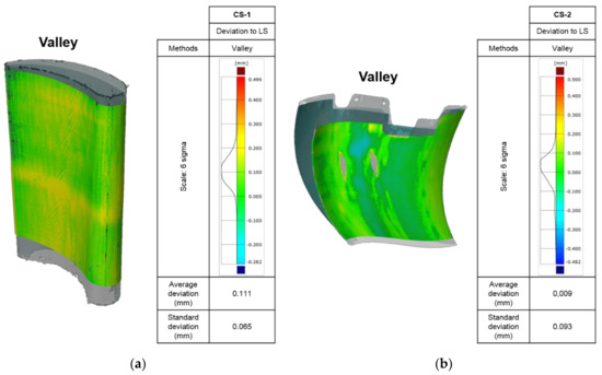
Figure 15.
Comparison of the obtained XRCT NURBS surfaces by applying the Valley thresholding method with the laser scan as the ground truth, for each case study: (a) CS-1; (b) CS-2.
Figure 15 exhibits that the deviation results for CS-1 (Figure 15a) are farther from the center than for CS-2 (Figure 15b), while the last one presents a wider range of values. Therefore, the achieved results are consistent with the results obtained in Section 3.3. For further analysis, the deviation results are summarized in Figure 16.
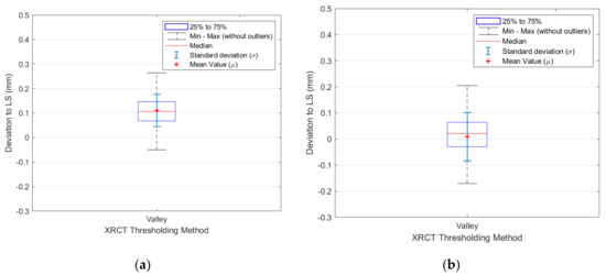
Figure 16.
Summarized results of the comparison of the obtained XRCT NURBS surfaces by applying the Valley thresholding method with the laser scan as the ground truth, for each case study: (a) CS-1; (b) CS-2.
In Figure 16, the mean value of the deviation results for CS-2 (Figure 16b) was reduced to approximately 8% of that obtained for CS-1 (Figure 16a), while the standard deviation was increased by around 43%. As stated above, this assessment is also related to the deviation analysis carried out in Section 3.3. The comparison between the results obtained in both sections reveals the following results. The mean value and the standard deviation of the obtained results for the NURBS surface generation increase by about 82% and 51% for CS-1 (Figure 16a). In other words, both features grow from 0.061 mm to 0.111 mm and from 0.043 mm to 0.065 mm, respectively. In contrast, for CS-2, the mean value decreases by around 47%, reaching 0.009 mm, while the standard deviation increases by about 5%, achieving 0.093 mm (Figure 16b). This effect is possibly caused because this procedure depends on different approaches that have their own influence on the outcomes, such as the distance between the sectioning planes, the curve approximation selected method and the sweep surface design operation, amongst others. Nonetheless, for both case studies the maximum mean value reached by this procedure is 0.111 mm, with standard deviation values below 0.100 mm.
4. Conclusions
In the present work, a RE methodology to achieve accurate polygon models and NURBS surfaces by applying different processing techniques was presented. From the research carried out, the following conclusions can be drawn:
- The proposed RE methodology reveals a promising future for achieving accurate polygon models for 3D printing or AM applications, as well as NURBS surfaces for advanced machining processes. This advantage allows design modifications, which is one of the most interesting challenges of a RE process.
- Apart from the data acquisition system and scanning conditions, the presented results suggest that the data processing step plays a major role in achieving accurate models of the scanned workpieces. In addition, the study demonstrates that the material and the geometry of the scanned workpiece also have their own effects on the outcomes, especially when using the XRCT data acquisition system.
- The developments of data processing techniques for achieving more accurate models from raw data are one of the current challenges of the RE process. In this context, the obtained results provide a first approach to the development of different data processing techniques in order to minimize error sources and offer more accurate models.
- The results achieved by applying the straightforward and fast computation methods proposed for image thresholding reveal that the accuracy of the obtained models depends on these calculated values. Therefore, the threshold value estimation provides the success of the presented RE methodology based on image processing techniques. For future research, the influence of applying more complex image processing techniques could be studied.
- In this framework, due to the results obtained for generating polygonal models, it could be well-founded to apply the Valley method in all case studies. Nonetheless, this method is strongly dependent on the histogram appearance, so its application might not be suitable in other circumstances.
- The deviation analysis between the polygon models shows that all the mean values reached by the proposed methods are below 0.100 mm, with 0.130 mm being the maximum standard deviation value out of all the case studies.
- The results obtained by using the Valley method for the NURBS surface generation reveal that the maximum mean value reached by this procedure is 0.111 mm, with standard deviation values below 0.100 mm for both case studies.
- Finally, the proposed methodology could be applied to any other data acquisition system that provides images or point clouds.
Author Contributions
Conceptualization, A.P., N.O. and S.P.; software, A.P.; validation, A.P., N.O. and S.P.; formal analysis, A.P.; investigation, A.P.; resources, N.O. and S.P.; data curation, A.P.; writing—original draft preparation, A.P.; writing—review and editing, A.P., N.O. and S.P.; visualization, A.P.; supervision, N.O., S.P., I.H. and J.I.A.; project administration, N.O., S.P., I.H. and J.I.A.; funding acquisition, N.O. and S.P. All authors have read and agreed to the published version of the manuscript.
Funding
This research was funded by the he Department of Economic Development, Sustainability and Environment of the Basque Government for funding the KK-2020/00094 (INSPECTA) research project and the Spanish Ministry of Science and Innovation for funding the ALASURF project (PID2019-109220RB-I00).
Acknowledgments
Special thanks are addressed to the Department of Economic Development, Sustainability and Environment of the Basque Government by funding the KK-2020/00094 (INSPECTA) research project. This work was also supported by the ALASURF project (PID2019-109220RB-I00) founded by Spanish Ministry of Science and Innovation.
Conflicts of Interest
The authors declare no conflict of interest.
References
- Gameros, A.; De Chiffre, L.; Siller, H.R.; Hiller, J.; Genta, G. A reverse engineering methodology for nickel alloy turbine blades with internal features. CIRP J. Manuf. Sci. Technol. 2015, 9, 116–124. [Google Scholar] [CrossRef]
- Bauer, F.; Schrapp, M.; Szijarto, J. Accuracy analysis of a piece-to-piece reverse engineering workflow for a turbine foil based on multi-modal computed tomography and additive manufacturing. Precis. Eng. 2019, 60, 63–75. [Google Scholar] [CrossRef]
- Yu, J.; Lynn, R.; Tucker, T.; Saldana, C.; Kurfess, T. Model-free subtractive manufacturing from computed tomography data. Manuf. Lett. 2017, 13, 44–47. [Google Scholar] [CrossRef]
- Paulic, M.; Irgolic, T.; Balic, J.; Cus, F.; Cupar, A.; Brajlih, T.; Drstvensek, I. Reverse engineering of parts with optical scanning and additive manufacturing. Procedia Eng. 2014, 69, 795–803. [Google Scholar] [CrossRef]
- Van Eijnatten, M.; Rijkhorst, E.J.; Hofman, M.; Forouzanfar, T.; Wolff, J. The accuracy of ultrashort echo time MRI sequences for medical additive manufacturing. Dentomaxillofac. Radiol. 2016, 45. [Google Scholar] [CrossRef]
- Huotilainen, E.; Jaanimets, R.; Valášek, J.; Marcián, P.; Salmi, M.; Tuomi, J.; Mäkitie, A.; Wolff, J. Inaccuracies in additive manufactured medical skull models caused by the DICOM to STL conversion process. J. Cranio-Maxillofac. Surg. 2014, 42. [Google Scholar] [CrossRef]
- Manmadhachary, A.; Ravi Kumar, Y.; Krishnanand, L. Improve the accuracy, surface smoothing and material adaption in STL file for RP medical models. J. Manuf. Process. 2016, 21, 46–55. [Google Scholar] [CrossRef]
- Pham, D.T.; Hieu, L.C. Reverse Engineering—Hardware and Software. In Reverse Engineering; Vinesh Raja, K.J.F., Ed.; Springer-Verlag London Limited: London, UK, 2008; pp. 33–70. ISBN 9781846288555. [Google Scholar]
- Chougule, V.N.; Mulay, A.V.; Ahuja, B.B. Development of patient specific implants for Minimum Invasive Spine Surgeries (MISS) from non-invasive imaging techniques by reverse engineering and additive manufacturing techniques. Procedia Eng. 2014, 97, 212–219. [Google Scholar] [CrossRef]
- Chougule, V.N.; Mulay, A.V.; Ahuja, B.B. Methodologies for Development of Patient Specific Bone Models from Human Body CT Scans. J. Inst. Eng. Ser. C 2016, 99, 413–418. [Google Scholar] [CrossRef]
- Modi, Y.K.; Sanadhya, S. Design and additive manufacturing of patient-specific cranial and pelvic bone implants from computed tomography data. J. Braz. Soc. Mech. Sci. Eng. 2018, 40, 1–11. [Google Scholar] [CrossRef]
- Li, L.; Li, C.; Tang, Y.; Du, Y. An integrated approach of reverse engineering aided remanufacturing process for worn components. Robot. Comput. Integr. Manuf. 2017, 48, 39–50. [Google Scholar] [CrossRef]
- Celentano, F.; Dipasquale, R.; Simoneau, E.; May, N.; Shahbazi, Z.; Shahbazmohamadi, S. Reverse Engineering and Geometric Optimization for Resurrecting Antique Saxophone Sound Using Micro-Computed Tomography and Additive Manufacturing. J. Comput. Inf. Sci. Eng. 2017, 17, 1–6. [Google Scholar] [CrossRef]
- Laycock, S.D.; Bell, G.D.; Corps, N.; Mortimore, D.B.; Cox, G.; May, S.; Finkel, I. Using a combination of micro-computed tomography, CAD and 3D printing techniques to reconstruct incomplete 19th-century cantonese chess pieces. J. Comput. Cult. Herit. 2015, 7, 2–7. [Google Scholar] [CrossRef]
- Momeni, F.M.; Hassani, N.S.M.M.; Liu, X.; Ni, J. A review of 4D printing. Mater. Des. 2017, 122, 42–79. [Google Scholar] [CrossRef]
- Werner, A.; Skalski, K.; Piszczatowski, S.; Świȩszkowski, W.; Lechniak, Z. Reverse engineering of free-form surfaces. J. Mater. Process. Technol. 1998, 76, 128–132. [Google Scholar] [CrossRef]
- Hayat, N.; Ahmad, M. The effects of computed tomography scanner parameters on the quality of the reverse triangular surface model of the fibula. J. Braz. Soc. Mech. Sci. Eng. 2016, 38, 21–31. [Google Scholar] [CrossRef]
- Kozior, T.; Bochnia, J.; Zmarzły, P.; Gogolewski, D. Waviness of Freeform Surface Characterizations from Austenitic Stainless Steel (316L) Manufactured by 3D Printing-Selective Laser Melting (SLM) Technology. Materials 2020, 13, 4372. [Google Scholar] [CrossRef]
- Kozior, T.; Bochnia, J. The influence of printing orientation on surface texture parameters in powder bed fusion technology with 316L steel. Micromachines 2020, 11, 639. [Google Scholar] [CrossRef]
- Heinzl, C.; Amirkhanov, A.; Kastner, J. Processing, analysis and visualization of CT data. In Industrial X-ray Computed Tomography; Carmignato, S., Dewulf, W., Leach, R., Eds.; Springer International Publishing AG: Cham, Switzerland, 2018; pp. 99–142. ISBN 9783319595733. [Google Scholar]
- Sezgin, M.; Sankur, B. Survey over image thresholding techniques and quanitative performance evaluation. J. Electron. Imaging 2004, 13, 146–168. [Google Scholar] [CrossRef]
- Lifton, J.J.; Liu, T. Evaluation of the standard measurement uncertainty due to the ISO50 surface determination method for dimensional computed tomography. Precis. Eng. 2020, 61, 82–92. [Google Scholar] [CrossRef]
- Otsu, N. A Threshold Selection Method from Gray-Level Histograms. IEEE Trans. Syst. Man. Cybern. 1979, 9, 62–66. [Google Scholar] [CrossRef]
- Rusu, R.B.; Marton, Z.C.; Blodow, N.; Dolha, M.; Beetz, M. Towards 3D Point cloud based object maps for household environments. Rob. Auton. Syst. 2008, 56, 927–941. [Google Scholar] [CrossRef]
- Lorensen, W.E.; Cline, H.E. Marching cubes: A high resolution 3D surface construction algorithm. In Proceedings of the 14th Annual Conference on Computer Graphics and Interactive Techniques SIGGRAPH 1987, Anaheim, CA, USA, 27–31 July 1987; Volume 21, pp. 163–169. [Google Scholar] [CrossRef]
- Schroeder, W.; Maynard, R.; Geveci, B. Flying edges: A high-performance scalable isocontouring algorithm. In Proceedings of the 2015 IEEE 5th Symposium on Large Data Analysis and Visualization (LDAV), Chicago, IL, USA, 25–26 October 2015; pp. 33–40. [Google Scholar] [CrossRef]
- Zhao, S.; Zhang, W.; Sheng, W.; Zhao, X. A Frame of 3D Printing Data Generation Method Extracted from CT Data. Sens. Imaging 2018, 19, 1–13. [Google Scholar] [CrossRef]
- Ryu, J.H.; Kim, H.S.; Lee, K.H. Contour-based algorithms for generating 3D CAD models from medical images. Int. J. Adv. Manuf. Technol. 2004, 24, 112–119. [Google Scholar] [CrossRef]
- Flöry, S. Fitting curves and surfaces to point clouds in the presence of obstacles. Comput. Aided Geom. Des. 2009, 26, 192–202. [Google Scholar] [CrossRef]
- Reinsch, C.H. Smoothing by spline functions. II. Numer. Math. 1967, 10, 177–183. [Google Scholar] [CrossRef]
- Yoo, D.J. Three-dimensional surface reconstruction of human bone using a B-spline based interpolation approach. CAD Comput. Aided Des. 2011, 43, 934–947. [Google Scholar] [CrossRef]
- Wang, W.; Pottmann, H.; Liu, Y. Fitting B-spline curves to point clouds by curvature-based squared distance minimization. ACM Trans. Graph. 2006, 25, 214–238. [Google Scholar] [CrossRef]
- Fan, J.L.; Lei, B. A modified valley-emphasis method for automatic thresholding. Pattern Recognit. Lett. 2012, 33, 703–708. [Google Scholar] [CrossRef]
- Stolfi, A.; De Chiffre, L.; Kasperl, S. Error sources. In Industrial X-ray Computed Tomography; Carmignato, S., Dewulf, W., Leach, R., Eds.; Springer International Publishing AG: Cham, Switzerland, 2018; pp. 143–184. ISBN 9783319595733. [Google Scholar]
- Spink, D.M. NURBS Toolbox by D.M. Spink 2020. Available online: https://www.mathworks.com/matlabcentral/fileexchange/26390-nurbs-toolbox-by-d-m-spink (accessed on 21 September 2020).
Publisher’s Note: MDPI stays neutral with regard to jurisdictional claims in published maps and institutional affiliations. |
© 2020 by the authors. Licensee MDPI, Basel, Switzerland. This article is an open access article distributed under the terms and conditions of the Creative Commons Attribution (CC BY) license (http://creativecommons.org/licenses/by/4.0/).