Dynamic Prediction Model for Uneven Slipper Wear Under Complex Lubrication Conditions Considering Lubrication–Wear Coupling

Abstract

It is difficult to experimentally determine the real-time wear coefficient of a slipper pair under complex lubrication conditions. To address this challenge, this study proposes a predictive method for slipper wear, eliminating the need for experimental measurement of the slipper pair’s friction coefficient under complex lubrication conditions. The force and motion characteristics of the slipper pair are analyzed to determine the non-uniform clearance distribution caused by elastic deformation and micro-motion. Based on the Greenwood–Williamson (G–W) model and Hertzian contact theory, the contact regions and stresses on the slipper bottom are accurately evaluated under mixed lubrication conditions. The Archard wear equation, combined with wear coefficients obtained from dry friction tests, is employed to calculate the instantaneous uneven wear of the slipper. This wear is then incorporated into iterative calculations of non-uniform clearance, forming a dynamic prediction model that captures the coupled relationship between lubrication and wear. The numerically simulated wear profile was compared with previously reported experimental measurements, and the discrepancies between them were analyzed. The results indicate that the proposed model can effectively predict the outer-side bottom wear of the slipper under steady-state operating conditions. Furthermore, the contact and wear behaviors under extreme conditions are investigated, the modeling results show revealing the variations in wear location and contact stress for ideal flat-bottom, low-speed, and high-speed operating states. The proposed model provides theoretical and methodological insights for optimizing the lubrication performance of slipper pairs during the stable wear stage.

1. Introduction

The slipper pair, as one of the three major friction pairs in swashplate axial piston pumps, is a primary force transmission component in these pumps [1,2,3,4]. The magnitude of the load it bears and the speed at which the load switches are no less than those experienced in a gun barrel at the moment of firing, indicating highly complex motion and loading conditions. The structure of the slipper pair is illustrated in Figure 1. The slipper pair consists of the swashplate, slipper, and the ball head of the piston, and the bottom of the slipper features a pocket and a bearing land. The slipper is connected to the piston via a ball joint and slides on the swashplate which forms an angle of β with the spindle axis. High-pressure oil from the piston chamber first passes through the damping hole in the piston ball head, then sequentially enters the ball joint, pocket, and the bearing land, where it forms an oil film between the swashplate and the slipper. The failure of the oil film on the bottom of the slipper is a significant cause of failures in axial piston pumps [5,6]. The lubrication performance of the slipper bottom directly influences the overall performance of axial piston pumps, representing a critical point for breakthrough in high-pressure and high-speed applications [7,8,9].

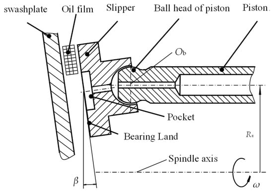
Figure 1. The structure of the slipper pair.

In engineering applications, users are more concerned about the slipper’s lubrication performance during the stable wear stage [10]. After running, the wear height of the bottom and the oil film thickness are within the same order of magnitude under mixed lubrication conditions. These are sensitive parameters that determine the slipper’s operating position and frictional power losses, among other lubrication properties of the bottom [11]. In order to design axial piston pumps with long life, high reliability, and superior performance, it is crucial to go beyond empirical formulas and trial-and-error design methods. Establishing a quantitative analysis model for slipper wear is urgently needed, which will provide computational analysis tools for the modern design of slipper pairs.

Achieving a profound understanding of the slipper pair’s motion characteristics is paramount to conducting research on slipper pairs [12,13]. Fisher conducted studies on the lubrication mechanisms of piston pump slipper pairs, discovering that under the influence of centrifugal torque, the slipper tilts slightly around the piston ball head. This tilt creates a bottom clearance that facilitates hydrodynamic lubrication, leading to an uneven distribution of oil film pressure between the slipper pair. The resultant counter-tilting torque can balance out the centrifugal force torque [14]. Researchers such as Harris R.M. from the University of Bath in the UK, through numerical computations, obtained curves depicting the maximum and minimum oil film thicknesses of the slipper pair over the operational cycle of the piston pump. Their findings indicated the presence of micro-movement of the slipper in the axial direction [15]. Scholars, including Hooke C.J. from the University of Birmingham in the UK, have pointed out that under the combined actions of ball joint friction force, centrifugal force, and bottom shear force, the slipper must incline to achieve a balance of moments. Centrifugal force causes the minimal point of the slipper bottom clearance to be located on the inner side of the slipper’s orbit. In the high-pressure oil zone, the friction force at the ball joint shifts the minimal point of clearance towards the outer side of the slipper’s orbit during its rotation, whereas in the low-pressure oil zone, it shifts towards the inner side [16,17,18]. Furthermore, the shear force acting on the slipper bottom positions the minimal clearance point at the leading edge of the slipper’s sliding path. In summary, it can be analyzed that the slipper pair undergoes a composite motion, involving rotation around its own axis, oscillation around the piston ball head, and reciprocating movement along the normal direction of its bottom [19,20].

To enhance lubrication performance of the slipper–swashplate interface in axial piston pumps, Wohlers A et al. adopted Automatic Dynamic Analysis of Mechanical System (ADAMS) software to develop dynamic models of pump components and utilized DSHplus software to establish a pressure response model for the hydraulic pump. Integrating the statistical method of surface roughness proposed by Partir and Cheng, they developed an average flow model and employed the G-W contact model to calculate the instantaneous pressures and contact forces between the slipper and swashplate during their interaction. This collective effort ultimately created a simulation model capable of depicting the tribological behavior of the slipper–swashplate system in a closed-axis piston pump [21]. Simultaneously, Canbulut F. et al. utilized the DSHplus program to perform predictive analyses on the oil film characteristics of the slipper pair [22,23]. They also designed a slipper testing device, which through experimentation effectively validated the inherent correlations between frictional power loss, oil leakage loss, slipper surface roughness, relative velocity, the size of pressure-bearing areas, supply oil pressure, and damper hole diameters.

The lubrication and wear processes of the slipper bottom exhibit a strong interdependence, forming a complex coupled system. Despite this recognition, quantitative analyses of wear based on the established contact models of the slipper’s bottom currently remain scarce. Ivantysyn R et al. have developed a wear prediction model based on the CASPAR simulation program to quantitatively analyze the skewed wear of the slipper bottom [24]. Du Z.L. et al. have established a method for predicting eccentric wear of the slipper, performing a quantitative analysis on key factors affecting wear, such as drain oil pressure, rotational speed, swashplate inclination angle, and oil viscosity, and their relationships with wear depth and width [25]. They found that the wear depth and width at the outer edge of the slipper bottom positively correlated with drain oil pressure and swashplate inclination angle, while negatively correlating with rotational speed and oil viscosity.

In summary, the micro-convex profile formed on the slipper pair’s bottom due to wear facilitates fluid lubrication between the slipper and the swashplate, and the worn profile in lubrication analysis aligns better with engineering practice and has been widely recognized [26]. Previous studies on the slipper pair’s force and motion characteristics, non-uniform clearance effects, coupled flow–solid–thermal modeling, and elastohydrodynamic lubrication provide a theoretical basis for this work.

However, challenges remain:

(1)

The complexity of the slipper’s dynamics makes it difficult to determine whether metal contact occurs, and, if so, the exact location and magnitude of the contact stresses.

(2)

The Archard wear model predicts material wear based on macroscopic parameters such as normal load, sliding distance, and material hardness. Yet the wear coefficient often requires experimental determination, and variations in lubrication performance under different operating conditions make it challenging to accurately determine real-time wear coefficients and instantaneous wear volume.

This work combines a dynamic lubrication model with Hertzian contact theory to obtain the direct metal-to-metal contact stress of the slipper pair, thereby enabling the incorporation of the wear coefficient under unlubricated conditions into the model to estimate the wear volume of the slipper bottom. For a slipper pair operating under complex lubrication conditions, this approach provides a more theoretically justified basis than assigning a constant wear coefficient under steady-state lubricated conditions.

2. Dynamic Uneven Wear Model

In swashplate axial piston pumps, the slipper pair plays a pivotal role in bearing, lubrication, and sealing, with its movement and loading conditions being intricate. As the rotational speed of the cylinder block increases and the working pressure rises, the interactions among multiple physical fields within the slipper pair become more pronounced. To accurately predict the interplay among the internal physical fields of the slipper pair and their lubrication performance, and to provide a theoretical foundation for analyzing slipper pair performance and optimizing the mechanism design, it is essential to delve into the coupling relationships among relevant parameters and establish a coupled model of the slipper pair.

2.1. Analysis of Slipper Motion

Assuming the slipper bottom is parallel to the swashplate, in Figure 2, a polar coordinate system (R, ϕ) with the swashplate surface center O_p as the pole is established to describe the slipper’s revolution motion. With the ball head center O_b of the piston as the origin, a Cartesian coordinate system (x, y) is set up, where the x-axis is tangent to the slipper sliding trajectory and points towards the negative sliding direction, and the y-axis is perpendicular to the slipper’s central sliding path and points outward from the swashplate, used to depict the tilting state of the slipper. Meanwhile, a cylindrical coordinate system (r, θ, z) centered at the bottom of the slipper O_s is established, the z-axis points in the direction of the oil film thickness of the slipper pair, θ starting from the x-axis and positive in the counterclockwise direction, to illustrate the slipper’s self-rotation and the distribution of physical fields such as clearance, pressure and stress. The main shaft rotates counterclockwise at an angular velocity ω, driving the piston and cylinder to rotate at the same angular velocity. The slipper, under the action of piston force and the retainer spring force, adheres to the swashplate. Owing to the tilt angle β between the swashplate and the main shaft, the slipper traces an elliptical path on the swashplate plane during revolution, with an angular velocity ω_s and revolution angle ϕ, the design starting point is the top dead point on the swashplate, and the direction is counterclockwise. In Figure 2, r₁ denotes the inner radius of the bearing land, and r₂ represents the outer radius.

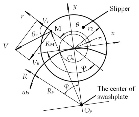
Figure 2. The motion of the slipper pair.

The circumferential velocity V of any point M on the bottom of the slipper bearing land in the polar coordinates is:

$$V={\omega }_{\mathrm{s}}{R}_{\mathrm{M}}$$

(1)

where ω_s is the angular velocity of the slipper’s revolution and R_M is the radius of any point M on the slipper bottom in the polar coordinates.

$${\omega }_{\mathrm{s}}=\omega {\displaystyle \frac{\cos \beta }{{\cos }^2\varphi +{\sin }^2\varphi {\cos }^2\beta }}$$

(2)

$$R_{\mathrm{M}}=\sqrt{r^2+R_{\mathrm{s}}^2+2r{R}_{\mathrm{s}}\cos (\theta -\pi /2)}$$

(3)

where R_s is the radius of the slipper’s center point in the polar coordinates.

$$R_{\mathrm{s}}=R_{\mathrm{z}}\sqrt{1+{\tan }^2\beta {\cos }^2\varphi }$$

(4)

where r is the radius of any point M on the bearing land in the cylindrical coordinate system (m), θ is the angle of any point M on the bearing land in the cylindrical coordinate system (rad), β is the swashplate inclination angle (rad), ϕ is the revolution angle of the slipper (rad), ω is the angular velocity of the piston ball head rotating around the drive shaft (rad/s), and R_z is the radius of the piston’s distribution in the cylinder (m).

The radial velocity V_r of any point M on the slipper bearing land in the cylindrical coordinate system is:

$$V_r=V\cos {\theta }_r$$

(5)

where θ_r is the angle between the slipper’s revolution line and the tangent of self-rotation.

$${\theta }_r=\arccos \left({\displaystyle \frac{R_{\mathrm{s}}\sin \left(\theta -\pi /2\right)}{R_{\mathrm{M}}}}\right)$$

(6)

Test results from the slipper self-rotation test rig constructed by Chao Q and his team at Zhejiang University indicate that the slipper’s self-rotation speed is approximately equal to the main shaft’s rotational speed. Based on the analysis from reference [27], the expression for the circumferential velocity V_θ of any point M in the cylindrical coordinate system is derived as follows:

$$V_{\theta }=V\sin {\theta }_r-{\omega }_{\mathrm{s}}r$$

(7)

2.2. Slipper Loading and Bearing Capacity

The loading and support of the slipper are shown in Figure 3, which ignores the component of friction force along the axis of the piston, and the dynamic characteristics of the oil film in the ball joint. It is assumed that the forces acting on the slipper include the retainer spring force, the inertial force of the piston-slipper pair, and the pressure from the pocket.

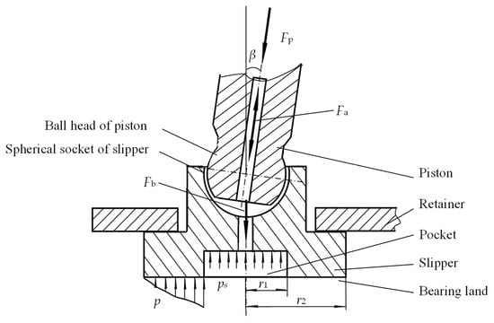
Figure 3. The loading and bearing capacity of the slipper.

The loading force F_N exerted on the slipper along the axial direction is:

$$F_{\mathrm{N}}=F_{\mathrm{b}}+{\displaystyle \frac{F_{\mathrm{p}}+F_{\mathrm{a}}}{\cos \beta }}$$

(8)

where F_b is the average force exerted by the center spring on the slipper (N), F_p is the load exerted by the piston (N), and F_a is the inertial force of the piston-slipper assembly (N):

$$F_{\mathrm{a}}=\left(m_{\mathrm{s}}+m_{\mathrm{p}}\right)R{\omega }^2\tan \beta \cos \varphi$$

(9)

$$F_{\mathrm{p}}=\pi r_{\mathrm{p}}^2{p}_{\mathrm{p}}$$

(10)

where r_p is the radius of the piston (m), m_s is the mass of the slipper (kg), m_p is the mass of the piston (kg), and p_p is the pressure in the piston chamber (Pa).

During operation, the slipper is subjected to spherical joint friction force and centrifugal force, causing it to incline. Hooke C J [16] studied the torque due to friction in the ball joint, analyzing how the friction force between the piston ball head and slipper socket induces slipper tilt. Liu Hong et al. [28] provided expressions for the friction-induced tilt torque generated by the interaction between the piston ball head and slipper socket, and the tilt torque components M_Bx and M_By in the coordinates of this study is:

$$\left\{\begin{array}{l}{M}_{\mathrm{B}x}=f_{\mathrm{bs}}{F}_{\mathrm{p}}{R}_{\mathrm{b}}\sin \varphi \sin \beta \\ M_{\mathrm{B}y}=f_{\mathrm{bs}}{F}_{\mathrm{p}}{R}_{\mathrm{b}}\cos \varphi \sin \beta \end{array}\right.$$

(11)

where f_bs is the equivalent friction coefficient of the ball joint, R_b is the radius of the ball head (m), and ϕ is the revolution angle of slipper (Rad).

The torque M_L resulting from the centrifugal force acting on the center of mass of the slipper is the outward tilting torque, which causes the slipper to tilt inward. The expression for M_L is as follows:

$$M_{\mathrm{L}}=m_{\mathrm{s}}{l}_{\mathrm{g}}{\omega }_{\mathrm{s}}^2{R}_{\mathrm{M}}$$

(12)

where l_g is the distance from the slipper’s center of gravity to the center of the piston ball head (m).

In Figure 3, p is the oil film pressure under the bearing land, which is calculated using the Reynolds lubrication equation. Reference [18] lists the Reynolds lubrication equation for incompressible fluids as follows:

$${\displaystyle \frac{1}{r}}{\displaystyle \frac{\partial }{\partial r}}\left(r{\displaystyle \frac{h^3}{\mu }}{\displaystyle \frac{\partial p}{\partial r}}\right)+{\displaystyle \frac{\partial }{r\partial \theta }}\left({\displaystyle \frac{h^3}{r\mu }}{\displaystyle \frac{\partial p}{\partial \theta }}\right)=6{\displaystyle \frac{1}{r}}{\displaystyle \frac{\partial }{\partial r}}\left(rh{V}_r\right)+6{\displaystyle \frac{\partial }{r\partial \theta }}\left(h{V}_{\theta }\right)+12{\displaystyle \frac{\partial h}{\partial t}}$$

(13)

The first two terms on the left side of the Reynolds equation represent fluid flow caused by pressure gradients, indicating that changes in fluid pressure will cause fluid motion. The first two terms on the right side of the equation represent fluid flow induced by the relative motion between the slipper and swashplate. The third term on the right represents fluid flow due to the variation over time of the clearance between the slipper and swashplate. Calculations of tribological properties such as load-bearing capacity, leakage, friction torque, and power loss of the slipper pair are all based on the pressure field calculations. The calculation of the pressure field can be achieved through numerically constructing a Reynolds discrete formulation and iterative solution.

The force exerted on the slipper by the piston ball head is balanced by the bearing force from the slipper’s bottom. This bearing force comprises two parts: the hydrostatic force from the pocket and the supporting force from the oil film under the bearing land. Assuming that the pressure in the pocket is uniformly distributed, F_S is [22]:

$$F_{\mathrm{S}}=p_{\mathrm{s}}\pi {r_1}^2+{\displaystyle {\int }_{r_1}^{r_2}{\displaystyle {\int }_0^{2\pi }prdrd\theta }}$$

(14)

where p_s is the pressure of pocket (Pa), r₁ is the inner radius of the bearing land (m), and r₂ is the outer radius of the bearing land (m).

The torques M_Sx and M_Sy produced by the normal stress and shear stress under the bearing land of slipper are [28]:

$$\left\{\begin{array}{l}{M}_{\mathrm{S}x}=-{\displaystyle {\int }_{r_1}^{r_2}{\displaystyle {\int }_0^{2\pi }p{r}^2\sin \theta drd\theta }}-l_{\mathrm{s}}{\displaystyle {\int }_0^{2\pi }{\displaystyle {\int }_{r_1}^{r_2}\left[{\tau }_{\mathrm{z}r}\sin \theta +{\tau }_{\mathrm{z}\theta }\cos \theta \right]}}rdrd\theta \\ M_{\mathrm{S}y}={\displaystyle {\int }_{r_1}^{r_2}{\displaystyle {\int }_0^{2\pi }p{r}^2\cos \theta drd\theta }}+l_{\mathrm{s}}{\displaystyle {\int }_0^{2\pi }{\displaystyle {\int }_{r_1}^{r_2}\left[{\tau }_{\mathrm{z}r}\cos \theta \right.}}\left.+{\tau }_{\mathrm{z}\theta }\sin \theta \right]rdrd\theta \end{array}\right.$$

(15)

where l_s is the distance from the bottom of the slipper to the center of the ball head (m), τ_zr is the radial shear stress at any point on the bearing land (N), and τ_zθ is the circumferential shear stress at any point on the bearing land (N).

The expressions for the radial shear stress and circumferential shear stress at any point on the bearing land are [29]:

$${\tau }_{\mathrm{z}r}={\displaystyle \frac{\partial p}{\partial r}}{\displaystyle \frac{h}{2}}+\mu {\displaystyle \frac{V_r}{h}}$$

(16)

$${\tau }_{\mathrm{z}\theta }={\displaystyle \frac{\partial p}{r\partial \theta }}{\displaystyle \frac{h}{2}}+\mu {\displaystyle \frac{V_{\theta }}{h}}$$

(17)

where μ is the viscosity of the oil film (Pa·s), and h is the clearance at any point on the bearing land (m).

A model for tilting contact of any circumferential section on bearing land is established, as depicted in Figure 4. After considering the influence of rough undersurface morphology, the probability of contact between rough peaks is higher at the position of small clearance on the bearing land. Figure 4a illustrates the tilting contact when the bearing land of slipper has a non-uniform clearance. In areas with smaller clearances, mixed lubrication exists between the swashplate and the slipper. Figure 4b provides a magnified view of any unit A_i,j in the mixed lubrication region of the bearing land of slipper. It is postulated that the upper reference plane of the oil film aligns with the equivalent surface of the slipper bearing land (the mean height line of the slipper’s roughness profile), taking roughness into account. Similarly, the lower reference plane of the oil film coincides with the equivalent surface of the swashplate (the mean height line of the swashplate’s roughness profile). It is further assumed that the oil film clearance across unit A_i,j is uniform, represented by the average clearance h_i,j.

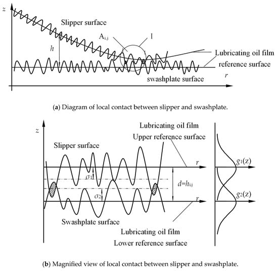
Figure 4. Tilting contact model of the slipper pair.

According to the assumptions proposed by Greenwood [30], the actual contact between the slipper and swashplate can be transformed into one involving a rigid smooth bottom and an elastic surface with rough peaks. Following this transformation of the contact situation between the slipper and the swashplate, the G-W contact model for unit A_i,j is depicted in Figure 5. In the illustration, it is assumed that the slipper’s bearing land acts as the rigid smooth bottom, while the swashplate serves as the rough reference surface. Within unit A_i,j, it is posited that the distance d, representing the distance between the rigid smooth bottom and the rough reference surface, is uniform and equals the average clearance h_i,j of the oil film. σ represents the RMS (Root Mean Square) of roughness after conversion. The shaded area indicates the elastic deformation of a single rough peak against the smooth rigid surface.

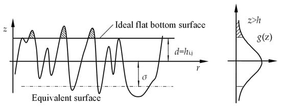
Figure 5. G-W contact model in unit A_i,j.

Neglecting the elastic interaction between rough peaks, based on the findings from literature [30], the metal contact stress formed by the rough peak contacts within unit A_i,j can be derived and expressed as:

$${\left.W\mathrm{w}\right|}_{\mathrm{i},\mathrm{j}}={\displaystyle \frac{4}{3}}N{\mathrm{E}}^{\prime }{R}_{\mathrm{w}1}^{1/2}{\displaystyle {\int }_{h\mathrm{i},\mathrm{j}}^{+\infty }{(z-h_{\mathrm{i},\mathrm{j}})}^{3/2}}g(z)dz$$

(18)

where N is the density of rough peaks (μm⁻²), R_w1 is the radius of curvature at the peak of rough peaks (μm). The height distribution of surface roughness peaks is described by the probability density function g(z), which follows either a Gaussian or non-Gaussian assumption [31,32]. The Gaussian distribution is given by [33]:

$$g(z)={\displaystyle \frac{1}{\sqrt{2\pi }\sigma }}{e}^{-{\displaystyle \frac{{(\mathrm{z}-\mu g)}^2}{2{\sigma }^2}}}$$

(19)

where μ_g is the mean value of the height distribution of surface roughness peaks, and ${\mathrm{E}}^{\prime }$ is combined elastic modulus, the expression is [34]:

$${\mathrm{E}}^{\prime }=1/\left({\displaystyle \frac{1-{\nu }_{\mathrm{e}1}^2}{{\mathrm{E}}_1}}+{\displaystyle \frac{1-{\nu }_{\mathrm{e}2}^2}{{\mathrm{E}}_2}}\right)$$

(20)

where ν_e1 is the Poisson’s ratio of the slipper material, and ν_e2 is the Poisson’s ratio of the swashplate material. under the G-W assumption, the RMS of roughness after conversion, according to literature [24], can be represented as:

$$\sigma =\sqrt{{\sigma }_1^2+{\sigma }_2^2}$$

(21)

where σ₁ is RMS of roughness on the swashplate surface (μm), σ₂ is RMS of roughness on the slipper surface (μm).

The above equations calculate the metal contact stress for any unit A_i,j of the slipper bearing land. Assuming a consistent distribution of slipper bearing land roughness parameters, substituting the corresponding values of the slipper bearing land’s clearance field h, a discrete expression for the contact force F_W can be obtained as:

$$F_{\mathrm{W}}={\displaystyle \sum _{\mathrm{i}=2}^{\mathrm{m}+1}{\displaystyle \sum _{\mathrm{j}=2}^{\mathrm{n}+1}}}{\left.f_{\mathrm{w}}\right|}_{\mathrm{i},\mathrm{j}}$$

(22)

where m is the number of radial grids on the slipper bearing land, matching the oil film grid parameters, n is the number of circumferential grids on the slipper bearing land, matching the oil film grid parameters.

2.3. Description of Non-Uniform Clearance

By disregarding the effects of surface roughness and thermal deformation, and by assuming that the swashplate surface is perfectly smooth and the structural stiffness is infinite, the expression for the clearance field h of the slipper bearing land can be defined as:

$$\mathit{h}={\mathit{h}}_{\mathrm{g}}+\Delta {\mathit{h}}_{\mathrm{m}}+\Delta {\mathit{h}}_{\mathrm{p}}$$

(23)

where h_g is the clearance field of an ideal flat bottom (m), Δh_m is the clearance field resulting from wear (m), and Δh_p is the clearance field induced by elastic deformation (m).

The description of ideal flat bottom with three points clearance is depicted in Figure 6. According to the principle of determining a plane using three points from literature [35], the clearances h₁, h₂, and h₃ at three points A₁, A₂, and A₃, located 120° apart along the outer edge of the bearing land, are utilized to ascertain the clearance h_g at any point on the bottom. This can be mathematically defined by the following formula [33]:

$$h_{\mathrm{g}}=(h_2-h_3){\displaystyle \frac{r\sin \theta }{\sqrt{3}{r}_2}}+\left(2h_1-h_2-h_3\right){\displaystyle \frac{r\cos \theta }{3r_2}}+{\displaystyle \frac{h_1+h_2+h_3}{3}}$$

(24)

where h₁ is the bottom clearance at the outer edge of the bearing land section at θ = 0° (m), h₂ is the bottom clearance at the outer edge of the bearing land section at θ = 120° (m), and h₃ is the bottom clearance at the outer edge of the bearing land section at θ = 240° (m), r₂ is the outer radius of the bearing land (m).

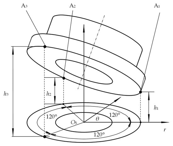
Figure 6. Description of ideal flat bottom with 3-Point clearance.

The wear depth of the bottom is typically of the same order of magnitude as the oil film thickness, making it a sensitive factor affecting the lubrication characteristics of the slipper pair. The Archard wear model is a commonly employed analytical tool for quantifying wear, considering macroscopic factors involved in sliding movements between two surfaces, such as normal load, sliding distances, and material hardness. Depending on the specific application scenario, like varying lubrication conditions, the wear coefficient often necessitates experimental determination. The lubrication performance of the slipper varies significantly under different operating conditions, wear states, and running orientations, making it challenging to precisely determine the real-time wear coefficient and instantaneous wear volume of the slipper–swashplate pair.

Wear on the bearing land is calculated using the Archard model, which considers metal contact stress and the experimental wear coefficient in the absence of lubrication. Without considering changes in surface chemical composition, the instantaneous wear rate dh_w of any unit A_i,j on the bearing land can be described as [36]:

$${\left.\mathrm{d}{h}_{\mathrm{w}}\right|}_{\mathrm{i},\mathrm{j}}=K_{\mathrm{w}}{\displaystyle \frac{{\left.W\mathrm{w}\right|}_{\mathrm{i},\mathrm{j}}}{H}}{\omega }_{\mathrm{s}}{R}_{\mathrm{M}}$$

(25)

where K_w is the experimental wear coefficient in the absence of lubrication, ω_s is the angular velocity of the slipper’s revolution, R_M is the radius of any point M on the bearing land in the revolving coordinate system, and H is the hardness of the softer material (MPa).

The wear behavior of the bearing land of slipper is characterized by changes in its wear depth. The contact wear volume dh_w is calculated using the Archard wear model, with the movement direction defaults to the normal direction of the contact surface. At the end of the k-th increment step, the real-time contact wear amount of the bearing land, $\Delta {\mathit{h}}_{\mathrm{m}}^{\mathrm{k}}$, can be obtained. For the subsequent time increment, the wear volume dh_w that satisfies iteration criteria will be applied to update the geometrical features $\Delta {\mathit{h}}_{\mathrm{m}}^{\mathrm{k}+1}$ of the wear on the bearing land, and the new wear profile $\Delta {\mathit{h}}_{\mathrm{m}}^{\mathrm{k}+1}$ of the bearing land will be recorded as:

$$\Delta {\mathit{h}}_{\mathrm{m}}^{\mathrm{k}+1}=\Delta {\mathit{h}}_{\mathrm{m}}^{\mathrm{k}}+\mathrm{d}{\mathit{h}}_{\mathrm{w}}$$

(26)

It can be observed that the wear of bearing land will alter the boundary condition of lubrication equation. Conversely, the lubrication equation will change the contact stress of the bottom because of the change in the boundary condition, and then affect the wear, forming the coupling relationship between lubrication and wear. This interdependency forms a coupled relationship between lubrication and wear, referred to as the lubrication-wear coupling.

The relationship between the forces applied to a horizontal plane and the resulting displacements in a semi-infinite body is depicted in Figure 7. When any grid A_r,t on the slipper’s bottom is subjected to a uniformly distributed force p_r,t, it induces a vertical displacement ${\left.\Delta h_{\mathrm{p}}\right|}_{\mathrm{i},\mathrm{j}}^{\mathrm{r},\mathrm{t}}$ in the horizontal plane of grid A_i,j. This displacement is inversely proportional to the distance ρ_ri between the two points. Additionally, other points on the bottom also contribute to the vertical displacement of the horizontal plane of grid A_i,j. When the entire slipper bearing land is influenced by a non-uniformly distributed stress, the vertical displacement at any point A_i,j on the surface can be calculated using the superposition principle. According to the literature [37], the discrete expression for the bearing land elastic deformation Δh_p is:

$${\left.\Delta h_{\mathrm{p}}\right|}_{\mathrm{i},\mathrm{j}}={\displaystyle \frac{\left(1-{v_1}^2\right)}{\pi E_1}}{\displaystyle \sum _{\mathrm{r}=1}^{\mathrm{m}}{\displaystyle \sum _{\mathrm{t}=1}^{\mathrm{n}+1}\frac{p_{\mathrm{r},\mathrm{t}}}{\sqrt{{r_{\mathrm{i}}}^2+{r_{\mathrm{r}}}^2-2r_{\mathrm{i}}{r}_r\cos {\theta }_{\mathrm{t}-\mathrm{j}}}}{r}_{\mathrm{r}}}}\Delta r\Delta \theta ,{r_{\mathrm{i}}}^2+{r_{\mathrm{r}}}^2-2r_{\mathrm{i}}{r}_r\cos {\theta }_{\mathrm{t}-\mathrm{j}}\ne 0$$

(27)

where E₁ is the Young’s modulus of the slipper material (Pa), p_r,t is the pressure distribution at the bearing land (Pa), m is the number of radial grids for the bearing land, n is the number of circumferential grids for the bearing land, and θ_t-j is the angle between points r_t and r_j (rad).

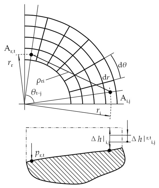
Figure 7. The diagram of force and displacement relationship of a semi-infinite body.

2.4. Pocket Flow Balance Equation

The depth of the pocket in the slipper is typically at the millimeter scale, which is a macroscopic parameter compared to the minute clearances under the bearing land. Thus, it is reasonable to assume that the pressure distribution throughout the pocket is uniform, with this pressure designated as p_s. Taking the volume formed by the pocket and the swashplate plane as the control volume V_s, hydraulic oil flows through the orifice in the piston, then through a fixed damping hole in the slipper, and subsequently enters the slipper’s pocket, it ultimately migrates through the narrow clearance between the slipper and the swashplate into the pump casing. According to the principle of mass conservation and considering the compressibility of the oil within the control volume, Wieczorek [38] has established a pressure equation for the pocket, which can be expressed as:

$${\displaystyle \frac{\mathrm{d}{p}_{\mathrm{s}}}{\mathrm{d}t}}={\displaystyle \frac{K}{V_{\mathrm{s}}}}(K_{\mathrm{s}}\left(p_{\mathrm{p}}-p_{\mathrm{s}}\right)-Q_{\mathrm{out}}-\pi {r_1}^2{\displaystyle \frac{d{h}_{\mathrm{o}}}{dt}})$$

(28)

$$V_{\mathrm{s}}=h_{\mathrm{s}0}\pi {r_1}^2$$

(29)

$$K_{\mathrm{s}}={\displaystyle \frac{\pi d_{\mathrm{c}}^4}{128\mu l_{\mathrm{c}}}}$$

(30)

where K is the bulk modulus of the oil (Pa), and h_o is the central clearance at the extended bottom of the bearing land (m). Q_out is the oil leakage flow from the pocket (m³/s), obtained through numerical computations. p_p is piston chamber pressure, V_s is the volume of pocket chamber, h_s0 is the height of the pocket (m), K_s is the pressure-flow coefficient of the damping holes in the slipper, d_c is the diameter of the damping hole (m), and l_c is the length of the damping hole (m).

By linking the surface elastic deformation equation with the oil film lubrication equation, a coupled relationship between pressure and clearance is established. Through the combination of the flow balance equation and the oil film lubrication equation, a coupled relationship between pressure and flow is formulated. Furthermore, by integrating the slipper bottom wear profile description equation with the oil film lubrication equation, a coupling between lubrication and wear processes is constructed.

3. Numerical Solution of Uneven Wear Model

The governing equation of the oil film in the slipper pair takes the form of an elliptic partial differential equation. Numerical solutions to such equations are typically obtained through spatial discretization using the finite difference method (FDM) or the finite volume method (FVM), both of which are intrinsically founded on the conservation of fluid mass flow. In this section, the lubrication equation is discretized and solved on the basis of the fluid flow conservation law.

The radial velocity v_r and circumferential velocity v_θ of the oil film at any point on the bottom surface of the slipper’s bearing land are given as follows:

$$v_r={\displaystyle \frac{1}{2\mu }}{\displaystyle \frac{\partial p}{\partial r}}\left(z^2-zh\right)+{\displaystyle \frac{V_{r}z}{h}}$$

(31)

$$v_{\theta }={\displaystyle \frac{1}{2\mu r}}{\displaystyle \frac{\partial p}{\partial \theta }}\left(z^2-zh\right)-{\displaystyle \frac{V_{\theta }\mathrm{z}}{h}}$$

(32)

By integrating the above two equations, the unit-width flow rates of the oil film on the bottom surface of the slipper’s bearing land in the radial and circumferential directions, q_r and q_θ, are obtained as follows:

$$q_r=-{\displaystyle \frac{h^3}{12\mu }}{\displaystyle \frac{\partial p}{\partial r}}+{\displaystyle \frac{V_{r}h}{2}}$$

(33)

$$q_{\theta }=-{\displaystyle \frac{h^3}{12\mu }}{\displaystyle \frac{\partial p}{r\partial \theta }}+{\displaystyle \frac{V_{\theta }h}{2}}$$

(34)

The mesh division of the oil film on the bottom surface of the slipper’s bearing land is shown in Figure 8. In the cylindrical coordinate system, the oil film region on the bottom surface of the bearing land is divided into m × n elements using a staggered grid. Each grid cell P is connected to its four neighboring cells. The solid points at the intersections of the dashed lines represent the nodes storing the pressure field p, while the hollow circles at the intersections of the solid lines represent the nodes storing the velocity field Vand the film thickness field h. $Q_{\mathrm{s}}$, $Q_{\mathrm{n}}$, $Q_{\mathrm{e}}$, $Q_{\mathrm{w}}$ denote the flow rates through the solid-line boundaries of grid P. The size of each staggered grid cell is determined by the radial width Δr and the circumferential width Δθ, which are defined as follows:

$$\Delta r={\displaystyle \frac{r_2-r_1}{\mathrm{m}}}$$

(35)

$$\Delta \theta ={\displaystyle \frac{2\pi }{\mathrm{n}}}$$

(36)

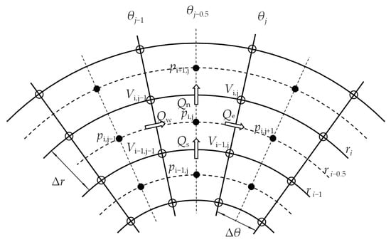
Figure 8. Mesh division beneath the slipper bearing land.

Since the velocity on the slipper bottom surface is a continuous function, the mean velocity along each solid-line segment is approximated by the velocity at its midpoint. Therefore, the average velocities on the four solid-line edges surrounding the grid center are calculated as the arithmetic averages of the velocities at the corresponding adjacent nodes. ${\stackrel{\_}{V_r}|}_{\mathrm{s}}$, ${\stackrel{\_}{V_r}|}_{\mathrm{n}}$, ${\stackrel{\_}{V_{\theta }}|}_{\mathrm{e}}$ and ${\stackrel{\_}{V_{\theta }}|}_{\mathrm{w}}$ are obtained as follows:

$${\stackrel{\_}{V_r}|}_{\mathrm{s}}={\left.V_r\right|}_{\mathrm{i}-1,\mathrm{j}-0.5}$$

(37)

$${\stackrel{\_}{V_r}|}_{\mathrm{n}}={\left.V_r\right|}_{\mathrm{i},\mathrm{j}-0.5}$$

(38)

$${\stackrel{\_}{V_{\theta }}|}_{\mathrm{e}}={\left.V_{\theta }\right|}_{\mathrm{i}-0.5,\mathrm{j}}$$

(39)

$${\stackrel{\_}{V_{\theta }}|}_w={\left.V_{\theta }\right|}_{\mathrm{i}-0.5,\mathrm{j}-1}$$

(40)

Similarly, the average film thickness can be expressed as follows:

$$h_{\mathrm{s}}=h_{\mathrm{i}-1,\mathrm{j}-1}+h_{\mathrm{i}-1,\mathrm{j}}$$

(41)

$$h_{\mathrm{n}}=h_{\mathrm{i},\mathrm{j}-1}+h_{\mathrm{i},\mathrm{j}}$$

(42)

$$h_{\mathrm{e}}=h_{\mathrm{i},\mathrm{j}}+h_{\mathrm{i}-1,\mathrm{j}}$$

(43)

$$h_{\mathrm{w}}=h_{\mathrm{i},\mathrm{j}-1}+h_{\mathrm{i}-1,\mathrm{j}-1}$$

(44)

Likewise, the first-order partial derivatives of pressure along each solid-line segment are approximated by the mid-point values within the corresponding segments. The first-order central difference method is employed to evaluate the pressure gradients along the grid solid-line segments, which can be expressed as:

$${\displaystyle \frac{\partial p}{\partial r}}{|}_{\mathrm{s}}={\displaystyle \frac{p_{\mathrm{i},\mathrm{j}}-p_{\mathrm{i}-1,\mathrm{j}}}{\Delta r}}$$

(45)

$${\displaystyle \frac{\partial p}{\partial r}}{|}_{\mathrm{n}}={\displaystyle \frac{p_{\mathrm{i}+1,\mathrm{j}}-p_{\mathrm{i},\mathrm{j}}}{\Delta r}}$$

(46)

$${\displaystyle \frac{\partial p}{r\partial \theta }}{|}_e={\displaystyle \frac{p_{\mathrm{i},\mathrm{j}+1}-p_{\mathrm{i},\mathrm{j}}}{r_{\mathrm{p}}\Delta \theta }}$$

(47)

$${\displaystyle \frac{\partial p}{r\partial \theta }}{|}_w={\displaystyle \frac{p_{\mathrm{i},\mathrm{j}}-p_{\mathrm{i},\mathrm{j}-1}}{r_{\mathrm{p}}\Delta \theta }}$$

(48)

Assuming the medium within grid P is incompressible, the flow conservation equation can be expressed as:

$$Q_{\mathrm{s}}-Q_{\mathrm{n}}+Q_{\mathrm{e}}-Q_{\mathrm{w}}=0$$

(49)

The flow rates across the four solid-line edges of grid P, denoted as $Q_{\mathrm{s}}$, $Q_{\mathrm{n}}$, $Q_{\mathrm{e}}$ and $Q_{\mathrm{w}}$, can be expressed, respectively, as follows:

$$Q_{\mathrm{s}}=-{\displaystyle \frac{h_{\mathrm{s}}^3\left(p_{\mathrm{i},\mathrm{j}}-p_{\mathrm{i}-1,\mathrm{j}}\right)r_{\mathrm{i}-1}\Delta \theta }{12\mu \Delta r}}+{\displaystyle \frac{{\stackrel{\_}{V_r}|}_{\mathrm{s}}{h}_{\mathrm{s}}{r}_{\mathrm{i}-1}\Delta \theta }{2}}$$

(50)

$$Q_{\mathrm{n}}=-{\displaystyle \frac{r_{\mathrm{i}}{h}_{\mathrm{n}}^3\left(p_{\mathrm{i}+1,\mathrm{j}}-p_{\mathrm{i},\mathrm{j}}\right)\Delta \theta }{12\mu \Delta r}}+{\displaystyle \frac{r_{\mathrm{i}}{\stackrel{\_}{V_r}|}_{\mathrm{n}}{h}_{\mathrm{n}}\Delta \theta }{2}}$$

(51)

$$Q_{\mathrm{e}}=-{\displaystyle \frac{h_{\mathrm{e}}^3\left(p_{\mathrm{i},\mathrm{j}}-p_{\mathrm{i},\mathrm{j}+1}\right)\Delta r}{12\mu r_{\mathrm{i}-0.5}\Delta \theta }}+{\displaystyle \frac{{\stackrel{\_}{V_{\theta }}|}_{\mathrm{e}}{h}_{\mathrm{e}}\Delta r}{2}}$$

(52)

$$Q_{\mathrm{w}}=-{\displaystyle \frac{h_{\mathrm{w}}^3\left(p_{\mathrm{i},\mathrm{j}-1}-p_{\mathrm{i},\mathrm{j}}\right)\Delta r}{12\mu r_{\mathrm{i}-0.5}\Delta \theta }}+{\displaystyle \frac{{\stackrel{\_}{V_{\theta }}|}_w{h}_{\mathrm{w}}\Delta r}{2}}$$

(53)

Substituting Equations (50)–(53) into Equation (49) and simplifying yields:

$$a_{\mathrm{p}}{p}_{\mathrm{i},\mathrm{j}}=a_{\mathrm{s}}{p}_{\mathrm{i}-1,\mathrm{j}}+a_{\mathrm{n}}{p}_{\mathrm{i}+1,\mathrm{j}}+a_{\mathrm{e}}{p}_{\mathrm{i},\mathrm{j}+1}+a_{\mathrm{w}}{p}_{\mathrm{i},\mathrm{j}-1}+b_p$$

(54)

The significance of each coefficient in the above equation is as follows:

$$a_{\mathrm{s}}={\displaystyle \frac{h_{\mathrm{s}}^3{r}_{\mathrm{s}}\Delta \theta }{\mu \Delta r}}$$

(55)

$$a_{\mathrm{n}}={\displaystyle \frac{h_{\mathrm{s}}^3{r}_{\mathrm{n}}\Delta \theta }{\mu \Delta r}}$$

(56)

$$a_{\mathrm{e}}={\displaystyle \frac{h_{\mathrm{s}}^3\Delta r}{{\mu }_{\mathrm{e}}{r}_{\mathrm{p}}\Delta \theta }}$$

(57)

$$a_{\mathrm{w}}={\displaystyle \frac{h_{\mathrm{e}}^3\Delta r}{{\mu }_{\mathrm{w}}{r}_{\mathrm{p}}\Delta \theta }}$$

(58)

$$b_{\mathrm{p}}=6\left(h_{\mathrm{s}}{\stackrel{\_}{V_r}|}_{\mathrm{s}}{r}_{\mathrm{s}}\Delta \theta -{\stackrel{\_}{h_{\mathrm{n}}{V}_r}|}_{\mathrm{n}}{r}_{\mathrm{n}}\Delta \theta +h_{\mathrm{w}}{\stackrel{\_}{V_{\theta }}|}_w\Delta r-h_{\mathrm{e}}{\stackrel{\_}{V_{\theta }}|}_{\mathrm{e}}\Delta r\right)$$

(59)

An iterative approach based on the successive over-relaxation (SOR) method is employed to solve the pressure field:

$$p_{\mathrm{i},\mathrm{j}}^{\mathrm{k}+1}=p_{i,j}^{\mathrm{k}}-{\psi }_{\mathrm{o}}\left({\displaystyle \frac{a_{\mathrm{p}}{p}_{\mathrm{i},\mathrm{j}}^{\mathrm{k}}-a_{\mathrm{s}}{p}_{\mathrm{i}-1,\mathrm{j}}^{\mathrm{k}+1}-a_{\mathrm{n}}{p}_{\mathrm{i}+1,\mathrm{j}}^{\mathrm{k}}-a_{\mathrm{e}}{p}_{\mathrm{i},\mathrm{j}+1}^{\mathrm{k}+1}-a_{\mathrm{w}}{p}_{\mathrm{i},\mathrm{j}-1}^{\mathrm{k}}-b_p}{a_{\mathrm{p}}}}\right)$$

(60)

where Ψ_o is the successive over-relaxation (SOR) factor for the pressure of the oil film on the slipper bearing surface. When Ψ_o is set between 1.58 and 1.7, relatively fast convergence can be achieved.

The convergence criterion for the numerical iterative solution is set as follows:

$${\epsilon }_{\mathrm{o}}={\displaystyle \sum _{\mathrm{i}=2}^{\mathrm{m}+1}{\displaystyle \sum _{\mathrm{j}=2}^{\mathrm{n}+1}\frac{p_{\mathrm{i},\mathrm{j}}^{\mathrm{k}+1}-p_{\mathrm{i},\mathrm{j}}^{\mathrm{k}}}{p_{\mathrm{i},\mathrm{j}}^{\mathrm{k}}}}}\le \left[{\epsilon }_{\mathrm{o}}\right]$$

(61)

where ε_o is the iteration error of the oil film pressure on the slipper support surface at the (k + 1)-th iteration. [ε_o] is the convergence tolerance for the oil film pressure iteration, which can be set to 1 × 10⁻⁴. When the iteration error satisfies the convergence tolerance, the solution of the oil film pressure field is considered complete.

By performing integration, the lubrication characteristics such as the supporting force of the slipper oil film, the dynamic pressure moment, and the leakage rate can be obtained. By approximating the partial derivatives with the first-order central difference scheme, the discrete expression for the leakage flow rate of the slipper pair can be derived as follows:

$$Q_{\mathrm{out}}={\displaystyle \sum _{\mathrm{j}=2}^{n+1}-\frac{h_{\mathrm{s}}^3\left(p_{\mathrm{i}+1,\mathrm{j}}-p_{\mathrm{i}-1,\mathrm{j}}\right)r_{\mathrm{s}}\Delta \theta }{6\mu \Delta r}+\frac{{\stackrel{\_}{V_r}|}_{\mathrm{s}}{h}_{\mathrm{s}}{r}_{\mathrm{s}}\Delta \theta }{2}}, \mathrm{i}\in (2\dots ,m)$$

(62)

The backward difference scheme is employed for the discretization of the unsteady term, and the discrete flow balance equation of the pocket is expressed as follows:

$${\displaystyle \frac{p_{\mathrm{s}}-p_{\mathrm{s}}^0}{\Delta t}}={\displaystyle \frac{K}{V_{\mathrm{s}}}}(K_{\mathrm{s}}\left(p_{\mathrm{p}}-p_{\mathrm{s}}\right)-Q_{\mathrm{out}}-\pi {r_1}^2{\displaystyle \frac{h_{\mathrm{o}}-h_{\mathrm{o}}^0}{\Delta t}})$$

(63)

In the equation, $p_{\mathrm{s}}^0$ denotes the pressure of the pocket at the previous time step, and $h_{\mathrm{o}}^0$ represents the central film thickness of the extended bottom surface of the support land at the previous time step.

After simplification, the discrete form of the pressure in the pocket is obtained as follows:

$$p_{\mathrm{s}}=\left[\Delta t{\displaystyle \frac{K}{V_{\mathrm{s}}}}(K_{\mathrm{s}}{p}_{\mathrm{p}}-Q_{\mathrm{out}}-\pi {r_1}^2{\displaystyle \frac{h_0-h_0^0}{\Delta t}})+p_{\mathrm{s}}^0\right]/\left(1+\Delta t{\displaystyle \frac{K{K}_{\mathrm{s}}}{V_{\mathrm{s}}}}\right)$$

(64)

An iterative solution for the pressure in the pocket is obtained using the successive over-relaxation (SOR) method:

$$p_{\mathrm{s}}^{\mathrm{k}+1}=p_{\mathrm{s}}^{\mathrm{k}}+{\psi }_{\mathrm{c}}\left(p_{\mathrm{s}}^{\mathrm{k}}-\overline{p_{\mathrm{s}}^{\mathrm{k}}}\right)$$

(65)

where ${\psi }_{\mathrm{c}}$ is the relaxation factor for the pressure iteration in the pocket.

$${\epsilon }_{\mathrm{c}}={\displaystyle \frac{p_{\mathrm{s}}^{\mathrm{k}+1}-p_{\mathrm{s}}^{\mathrm{k}}}{p_{\mathrm{s}}^{\mathrm{k}}}}\le \left[{\epsilon }_{\mathrm{c}}\right]$$

(66)

where ε_c is the iteration error of the oil film pressure on the slipper support surface at the (k + 1)-th iteration. [ε_c] is the convergence tolerance for the oil film pressure iteration, which can be set to 1 × 10⁻⁴. The pressure at the center of each grid cell is used to approximate the average pressure within the cell, and the discrete equation for the supporting force on the bottom surface of the slipper support land is obtained as follows:

$$F_{\mathrm{S}}=p_{\mathrm{s}}\pi {r_1}^2+{\displaystyle \sum _{\mathrm{i}=2}^{\mathrm{m}+1}{\displaystyle \sum _{\mathrm{j}=2}^{\mathrm{n}+1}{p}_{\mathrm{i},\mathrm{j}}{r}_{i-0.5}\Delta r}}\Delta \theta$$

(67)

Assuming that the pressure, film thickness, and velocity at the grid center represent the average values within each cell, the discrete form of the tilting moment resistance acting of the slipper bearing land can be expressed as follows:

$$M_{\mathrm{S}x}={\displaystyle \sum _{\mathrm{i}=2}^{\mathrm{m}+1}{\displaystyle \sum _{\mathrm{j}=2}^{\mathrm{n}+1}{p}_{\mathrm{i},\mathrm{j}}\sin \left[\left(j-0.5\right)\Delta \theta \right]{r_{\mathrm{p}}}^2\Delta r}}\Delta \theta +{\displaystyle \sum _{\mathrm{i}=2}^{\mathrm{m}+1}{\displaystyle \sum _{\mathrm{j}=2}^{\mathrm{n}+1}{l}_{\mathrm{s}}\left({\left.{\tau }_{zrx}\right|}_{\mathrm{i},\mathrm{j}}-{\left.{\tau }_{z\theta x}\right|}_{\mathrm{i},\mathrm{j}}\right)r_{\mathrm{p}}\Delta r\Delta \theta }}$$

(68)

$$M_{\mathrm{S}y}={\displaystyle \sum _{\mathrm{i}=2}^{\mathrm{m}+1}{\displaystyle \sum _{\mathrm{j}=2}^{\mathrm{n}+1}{p}_{\mathrm{i},\mathrm{j}}{r_{\mathrm{p}}}^2\cos \left[\left(j-0.5\right)\Delta \theta \right]\Delta r}}\Delta \theta +{\displaystyle \sum _{\mathrm{i}=2}^{\mathrm{m}+1}{\displaystyle \sum _{\mathrm{j}=2}^{\mathrm{n}+1}{l}_{\mathrm{s}}\left({\left.{\tau }_{zry}\right|}_{\mathrm{i},\mathrm{j}}+{\left.{\tau }_{z\theta y}\right|}_{\mathrm{i},\mathrm{j}}\right)r_{\mathrm{p}}\Delta r\Delta \theta }}$$

(69)

The components of the shear stress in the radial and circumferential directions at the center point of the A_i,j, denoted as ${\left.{\tau }_{zrx}\right|}_{\mathrm{i},\mathrm{j}}$, ${\left.{\tau }_{z\theta x}\right|}_{\mathrm{i},\mathrm{j}}$, ${\left.{\tau }_{zry}\right|}_{\mathrm{i},\mathrm{j}}$ and ${\left.{\tau }_{z\theta y}\right|}_{\mathrm{i},\mathrm{j}}$ can be expressed, respectively, as follows:

$${\left.{\tau }_{zrx}\right|}_{\mathrm{i},\mathrm{j}}=\left({\displaystyle \frac{p_{\mathrm{i}+1,\mathrm{j}}-p_{\mathrm{i}-1,\mathrm{j}}}{2\Delta r}}{h}_{\mathrm{p}}+{\displaystyle \frac{\mu {\left.V_r\right|}_{\mathrm{p}}}{h_{\mathrm{p}}}}\right)\cos \left[\left(j-0.5\right)\Delta \theta \right]$$

(70)

$${\left.{\tau }_{z\theta x}\right|}_{\mathrm{i},\mathrm{j}}=\left({\displaystyle \frac{p_{\mathrm{i},\mathrm{j}+1}-p_{\mathrm{i},\mathrm{j}-1}}{2\Delta r}}{h}_{\mathrm{p}}+{\displaystyle \frac{\mu {\left.V_{\theta }\right|}_{\mathrm{p}}}{h_{\mathrm{p}}}}\right)\cos \left[{\displaystyle \frac{\pi }{2}}-\left(j-0.5\right)\Delta \theta \right]$$

(71)

$${\left.{\tau }_{zry}\right|}_{\mathrm{i},\mathrm{j}}=\left({\displaystyle \frac{p_{\mathrm{i}+1,\mathrm{j}}-p_{\mathrm{i}-1,\mathrm{j}}}{2\Delta r}}{h}_{\mathrm{p}}+{\displaystyle \frac{\mu {\left.V_r\right|}_{\mathrm{p}}}{h_{\mathrm{p}}}}\right)\sin \left[\left(j-0.5\right)\Delta \theta \right]$$

(72)

$${\left.{\tau }_{z\theta y}\right|}_{\mathrm{i},\mathrm{j}}=\left({\displaystyle \frac{p_{\mathrm{i},\mathrm{j}+1}-p_{\mathrm{i},\mathrm{j}-1}}{2\Delta r}}{h}_{\mathrm{p}}+{\displaystyle \frac{\mu {\left.V_{\theta }\right|}_{\mathrm{p}}}{h_{\mathrm{p}}}}\right)\sin \left[{\displaystyle \frac{\pi }{2}}-\left(j-0.5\right)\Delta \theta \right]$$

(73)

3.1. Objective Function

Considering the impact of the torque generated by its rotational inertia, the equilibrium equations for force and torque of slipper take the form:

$$f_1\left(\mathit{h},{\mathit{h}}^{\prime },t\right)=F_{\mathrm{S}}\left(\mathit{h},{\mathit{h}}^{\prime },t\right)+F_{\mathrm{X}}\left(\mathit{h},{\mathit{h}}^{\prime },t\right)+F_{\mathrm{W}}\left(\mathit{h},{\mathit{h}}^{\prime },t\right)-F_{\mathrm{N}}\left(t\right)=0$$

(74)

$$f_2\left(\mathit{h},{\mathit{h}}^{\prime },t\right)=M_{\mathrm{S}x}\left(\mathit{h},{\mathit{h}}^{\prime },t\right)+M_{\mathrm{X}x}\left(\mathit{h},{\mathit{h}}^{\prime },t\right)+M_{\mathrm{W}x}\left(\mathit{h},{\mathit{h}}^{\prime },t\right)-M_{\mathrm{B}x}\left(t\right)-M_L\left(t\right)-I_x(\mathit{h},{\mathit{h}}^{\prime },t)=0$$

(75)

$$f_3\left(\mathit{h},{\mathit{h}}^{\prime },t\right)=M_{\mathrm{S}y}\left(\mathit{h},{\mathit{h}}^{\prime },t\right)+M_{\mathrm{X}y}\left(\mathit{h},{\mathit{h}}^{\prime },t\right)+M_{\mathrm{W}y}\left(\mathit{h},{\mathit{h}}^{\prime },t\right)-M_{\mathrm{B}y}\left(t\right)-I_y(\mathit{h},{\mathit{h}}^{\prime },t)$$

(76)

These equations encompass seven variables, including the clearances h₁, h₂, and h₃, at three reference points, each 120° apart along the outer edge of the ideal flat bottom, the clearance changes h₁′, h₂′, and h₃′, and time t. The clearances at these three reference points (h₁, h₂, h₃) are represented by the vector h, while the clearance changes (h₁′, h₂′, h₃′) are expressed by the vector h′. In a discrete algorithm, once the time step is determined, the variable t is accordingly fixed. This establishes a definitive correspondence between h and h′.

The objective function can be constructed as:

$$\min (\mathit{f}\left({\mathit{h}}^{\prime }\right))=f_1\left({\mathit{h}}^{\prime }\right)/F_{\mathrm{N}}(t)+f_2\left({\mathit{h}}^{\prime }\right)/\left(M_{\mathrm{B}x}\left(t\right)-M_L\left(t\right)\right)+f_3\left({\mathit{h}}^{\prime }\right)/M_{\mathrm{B}y}\left(t\right)$$

(77)

The convergence criterion for the numerical iterative solution is set as:

$${\mathrm{E}}_{\mathrm{n}}=\mathit{f}\left({\mathit{h}}^{\prime }\right)\le \left[{\epsilon }_{\mathrm{f}}\right]$$

(78)

where [ε_f] is the convergence precision of the objective function.

3.2. Boundary Condition Settings

The numerical discretization process is primarily focused on internal nodes, whereas boundary nodes or external nodes require assigned values or interpolation from internal nodes [39]. The numerical model’s boundary conditions are illustrated in Figure 9.

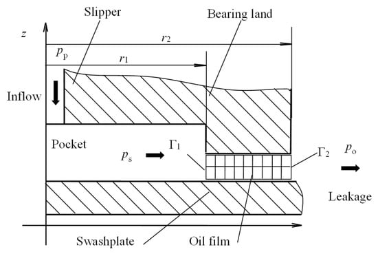
Figure 9. Diagram of boundary conditions.

The slipper bearing land has four pressure boundaries, designated as Г₁, Г₂, θ = 0, and θ = 2π planes. At Г₁, the pressure at each node equals the pressure within the pressurized chamber p_s. Similarly, at Г₄, the pressure at every node matches the casing pressure p_o. For all the nodes coinciding on the θ = 0 and θ = 2π plane in cylindrical coordinates, the expressions are [40]:

$${\left.p\right|}_{\Gamma ={\Gamma }_1}={\left.p_s\right|}_{r=r_1}$$

(79)

$${\left.p\right|}_{\Gamma ={\Gamma }_4}={\left.p_{\mathrm{o}}\right|}_{r=r_2}$$

(80)

$${\left.p\right|}_{\theta =0}={\left.p\right|}_{\theta =2\pi }$$

(81)

p_p is displacement chamber pressure, the time-varying expression can be presented as [41]:

$$p_{\mathrm{p}}=\left\{\begin{array}{l}-{\displaystyle \frac{K{A}_{\mathrm{p}}}{V_0+A_{\mathrm{p}}s}}{\displaystyle \frac{ds}{d\theta }}\left(j\cdot \Delta \theta \right)\left(0\le j\le 10\right)\\ p_{\mathrm{o}}\left(10\le j\le 170\right)\\ p_{\mathrm{o}}-{\displaystyle \frac{K{A}_{\mathrm{p}}}{V_0+A_{\mathrm{p}}s}}{\displaystyle \frac{ds}{d\theta }}\left[\left(j-170\right)\cdot \Delta \theta \right]\left(170\le j\le 180\right)\\ p_{\mathrm{i}}\left(180\le j\le 360\right)\end{array}\right.$$

(82)

where V₀ is the initial volume of the piston chamber; A_p is the area of the piston chamber; p_o is the working pressure; K is the volume modulus; j is the number; θ is the shaft rotational angle; ∆θ is the rotational angle increment.

4. Comparison to Measurement

Ivantysyn [24] built a slipper wear test under specific operating conditions and obtained post-wear profiles of the bearing land. In this paper, utilizing the G-W roughness model combined with Hertzian contact theory, the contact positions, areas, and stress magnitudes on the bearing land under mixed lubrication conditions are calculated in real-time based on the distribution of interfacial clearances. The structural parameters of the slipper pair considering surface roughness are listed in Table 1. The set up for single bearing land of slipper wear simulation test conditions is presented in Table 2, encompassing extreme operating scenarios such as low-pressure-high-speed and high-pressure-low-speed conditions. With each simulation condition running for an hour, to obtain the worn profiles of the bearing land. To reduce computational runtime, an acceleration wear factor was implemented in the program, and a dimensionless radius $\overline{r}$ was defined as:

$$\overline{r}={\displaystyle \frac{r-r_1}{r_2}}$$

(83)

Table 1. The basic parameters of the slipper considering surface roughness.

Parameters	Unit	Value	Parameters	Unit	Value
Inside radius of slipper bearing land (r1)	mm	7.9	Outer radius of piston (rp)	mm	9.5
Outside radius of slipper bearing land (r2)	mm	11.2	Distribution circle radius of piston (Rz)	mm	44
Radius of piston ball head (Rb)	mm	7	Equivalent friction coefficient of spherical joint (fbs)	-	0.1
Slipper mass (ms)	kg	0.014	Offset of slipper center of gravity (lg)	mm	17
Piston mass (mp)	kg	0.08	Distance from slipper bottom to ball head center (ls)	mm	22
Slipper torque of inertia (Jx)	kgm2	0.021	Slipper torque of inertia (Jy)	kgm2	0.021
Poisson’s ratio of slipper (νe1)	-	0.32	Elastic modulus of slipper (E1)	GPa	108
Poisson’s ratio of swashplate (νe2)	-	0.25	Elastic modulus of swashplate (E2)	GPa	206
Slipper bottom wear profile parameters (Δh1)	μm	0	swashplate inclination angle (β)	°	14
Slipper bottom wear profile parameters (Δh2)	μm	2	Vertex parameters of wear profile (λr)	-	0.1
Thickness of slipper (Hs)	mm	4	Height of pocket hs0)	mm	2
Damping hole length of slipper (lc)	mm	3.5	Diameter of slipper damping hole (dc)	mm	1.5
Wear coefficient (Kw)	-	5 × 10−4	Density of roughness peaks (N)	μm−2	1.77 × 10−3
Root mean square value of surface roughness peaks on the slipper (σ2)	μm	0.574	Root mean square value of swashplate surface roughness peaks (σ1)	μm	0.574
Curvature radius at the top of roughness peak (Rw1)	μm	35.84	Hardness of slipper material (H)	MPa	850

Table 2. Simulation operating parameter of slipper wear test.

Operating Conditions Number	Pressuyre	Cylinder Block Rotational Speed	Operating Duration	Operating Conditions Number	Pressure	Cylinder Block Rotational Speed	Operating Duration
	MPa	Rad	h		MPa	Rad	h
OC1	5	500 × 2π/60	1	OC2	10	500 × 2π/60	1
OC3	20	500 × 2π/60	1	OC4	30	500 × 2π/60	1
OC5	5	750 × 2π/60	1	OC6	10	750 × 2π/60	1
OC7	20	750 × 2π/60	1	OC8	30	750 × 2π/60	1
OC9	20	1000 × 2π/60	1	OC10	30	1000 × 2π/60	1
OC11	30	1250 × 2π/60	1	OC12	5	3000 × 2π/60	1
OC13	10	3000 × 2π/60	1	OC14	20	3000 × 2π/60	1
OC15	25	3000 × 2π/60	1	OC16	30	3000 × 2π/60	1

Figure 10 shows a comparison of bottom wear on a single bearing land slipper under different operating conditions, which revealed that wear mainly occurs under low-speed high-pressure and high-speed low-pressure conditions.

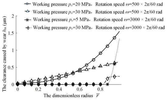
Figure 10. Comparison of bottom wear on a single bearing land slipper under different operating conditions.

Figure 11 shows a comparison between the simulation results of this study and the previously reported experimental measurements. After three test cycles, the measured wear profile of the slipper’s bearing land is represented by the solid line in the figure. Since this simulation only considered steady-state operating conditions and did not take into account the structural stiffness of the slipper, dynamic load variations, cavitation corrosion, or wear caused by contaminant particles during actual operation, it is quite likely that during cold starts or highly dynamic conditions, such as rapid swashing, the slipper tilt increases and wears even more. Therefore, a noticeable discrepancy appears between the simulated wear profile on the inner side of the bearing land (especially in terms of wear depth) and the experimental results reported in [24] (shown by the dashed line in Figure 11). The detailed explanations for these differences have been thoroughly discussed by Ivantysyn [24]. Nevertheless, the profile on the outer edge seems to follow the overall trend very well. The outer edge appears to be more severely worn than that in the measurement results, which may be attributed to the fact that the experimental data were obtained using a profilometer and did not account for the cumulative wear height of the slipper. Overall, the simulation results of this study are consistent with those reported in [24], indicating that the developed dynamic non-uniform wear model can effectively predict the outer-side bottom wear of the slipper under steady-state operating conditions.

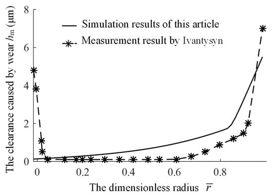
Figure 11. Comparison between the simulation results and the existing measured results.

5. Analysis of Bearing Land Wear Under Extreme Conditions

5.1. Wear on the Ideal Flat Bearing Land

E. Koc [17] points out that an ideal flat bottom slipper cannot achieve force and torque balance under lubrication conditions, which will lead to forward tilting operation, causing the bearing land to encounter the swashplate. In this section, elastic deformation is considered to analyze the operational posture and wear of the slipper with an ideal flat bearing land. The ideal flat bearing land mentioned in this section does not consider the effects of machining errors, surface roughness, and surface wear profiles, so the above parameters are not taken into account in Table 1. The operating parameters are shown in Table 3.

Table 3. Simulation operation parameters.

Parameters	Symbols	Value	Unit
Piston load pressure	pp	21	MPa
Casing pressure	po	0.2	MPa
Cylinder block rotational speed	ω	300 × 2π/60	Rad
Retainer pressure	Fb	100	N

Figure 12 illustrates how these three clearances (h₁, h₂, and h₃) at the outer edge of bearing land vary with the rotation angle of the cylinder block. As the cylinder block rotates 360°, the slipper slides one full cycle on the swashplate surface, with the first half of the cycle predominantly under high pressure and the latter half mainly experiencing low pressure. The sliding range where the slipper undergoes high pressure can be termed the high-pressure zone, while the range under low pressure is the low-pressure zone. The intervals between these zones can be referred to as the low-pressure-to-high-pressure transition zone and the high-pressure-to-low-pressure transition zone, respectively. Below are the features of the variation in the three-point clearances at the outer edge of bearing land as the cylinder block rotates between 0° and 1800°.

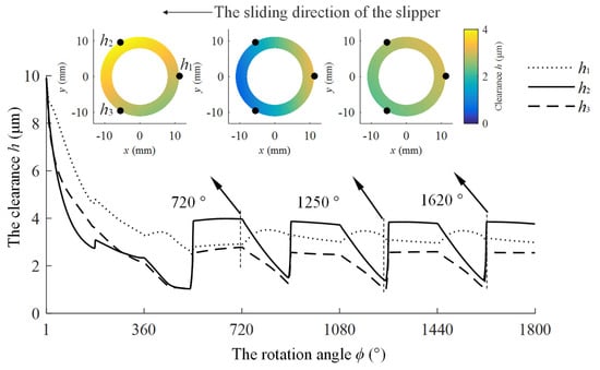
Figure 12. Variation in the clearances at three points on the ideal flat bearing land of the slipper.

In the range of 0–530°, among the three reference points on the outer edge of bearing land, point A₁ exhibits the largest clearance value h₁ among the three, indicating a forward-tilted running posture of the slipper. At this stage, the bearing land cannot provide wedge hydrodynamic lubrication pressure. The clearances at all three reference points gradually decrease with the rotation of the cylinder block, suggesting that the slipper’s bearing land is continuously compressing the oil film. It relies on the squeezing effect of the oil film and the uneven distribution of static pressure lubrication pressures across the inclined bottom to counterbalance the clamping force of the piston and the tilting torque. Ultimately, this leads to metal-to-metal contact between the bearing land and the swashplate.

In the range of 530–546°, the slipper traverses the high-pressure to low-pressure transition zone, during which the piston clamping force progressively decreases towards the casing pressure. The bearing land elastically recovers, and in this recovery process, a significant elastic contact force is generated, causing the contacting end to rebound rapidly. This is reflected in the figure by a swift increase in the clearance h₂ at point A₂ and clearance h₃ at point A₃, indicating a sudden widening of these clearances as the slipper’s surface bounces back.

In the range of 546–720°, as the slipper traverses the low-pressure zone, it experiences reduced clamping force and primarily undergoes a rearward tilting torque. Due to the rebound and subsequent rearward tilt of the slipper, the bottom of the bearing land forms a wedge-shaped hydrodynamic lubrication effect, which helps to balance part of the clamping force and the rearward tilting torque. As depicted in the figure, the clearance h₁ at point A₁ on the outer edge of the bearing land becomes less than the clearance h₂ at point A₂.

In the range of 720–730°, as the slipper crosses the low-pressure to high-pressure transition zone, the clamping force from the piston and the forward tilting torque sharply increase. Meanwhile, the oil film beneath the slipper’s bearing land in this zone is relatively thick, leading to a weaker wedge hydrodynamic effect. In order to balance the rapidly increasing piston clamping force, the slipper needs to shift downward as a whole to provide compressive force, and in order to counterbalance the increased forward tilting torque, the slipper must incline forward to alter the pressure distribution and generate a counteracting forward tilting torque. As depicted in the figure, the clearances h₂ at point A₂ and h₃ at point A₃ on the outer edge of the slipper’s bearing land decrease, while the clearance h₁ at point A₁ increases.

In the range of 730–810°, as the slipper moves through the front of the high-pressure zone, the forward tilting torque it experiences gradually decreases, causing the slipper to tilt forward at a slower rate. Meanwhile, in adherence to the residual clamping force design criteria, the slipper continues to provide compressive force to balance the piston clamping force. This scenario is depicted in the figure by a reduction in the clearances h₂ at point A₂ and h₃ at point A₃ on the outer edge of the slipper’s bearing land, while the increase in the clearance h₁ at point A₁ slows down.

In the range of 810–900°, as the slipper proceeds through the back of the high-pressure zone, the frictional torque from the piston transitions from a forward tilting torque to a rearward one, which steadily increases. This is observable in the figure where the clearances h₂ at point A₂ and h₃ at point A₃ on the outer edge of the slipper’s bearing land continue to decrease, while the clearance h₁ at point A₁ switches from increasing to decreasing. Subsequently, the clearances at the three points around the outer edge of bearing land exhibit periodic variations, with these changes basically stabilizing after 1440°.

From Figure 12, it is evident that under the residual clamping force design principle, even when accounting for elastic deformation, the assumption of an ideal flat bottom fails to achieve force and torque balance under full lubrication conditions. Consequently, the slipper will operate in a cycle characterized by contact-rebound-contact.

The variation in the minimum clearance on the bearing land with cylinder rotation angle is depicted in Figure 13, it shows the variation in the minimum clearance of the bearing land during with a cylinder block rotation angle of 0–1800°. The minimum clearance of the bearing land varies periodically. The example below illustrates one operating cycle for the range of 1440° to 1800°.

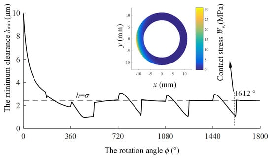
Figure 13. Curve of minimum clearance variation with cylinder block rotation angle.

In the range of 1440–1450°, as the slipper traverses the low-pressure to high-pressure transition zone, the high-pressure oil from the piston chamber causes the bearing land to deform under pressure, leading to a rapid increase in the minimum clearance.

In the range of 1450–1610°, as the slipper moves through the high-pressure zone, it needs the slipper to continually descend to compress the oil film to balance the residual clamping force. The curve of the minimum clearance of the slipper’s bearing land decreases gradually with the rotation of the cylinder block. When the cylinder block’s rotation angle reaches 1530°, the minimum clearance of the bearing land is less than three times the RMS roughness (indicated by the dashed line in the figure). The bearing land is in a mixed lubrication state and will experience contact wear.

In the range of 1610–1626°, as the slipper crosses the high-pressure to low-pressure transition zone, the volume of the piston chamber increases and pressure drops abruptly. This prompts an elastic recovery of the slipper’s bearing land. During this recovery, larger elastic reaction forces are generated, causing the contacting portion to spring back rapidly. Consequently, in this phase, the curve of the bearing land minimum clearance initially plunges swiftly but then rebounds rapidly upward.

In the range of 1626–1800°, as the slipper passes through the low-pressure region, it primarily bears the clamping force from the central spring, which acts to restrain the slipper from lifting off the swashplate. Meanwhile, the hydrodynamic lubrication effect is relatively weak in this area. Hence, the curve representing the minimum clearance of the bearing land does not continue to rise.

There is a large amount of metal contact deformation on the slipper’s bearing land when the cylinder block rotation angle is 1612°, and the corresponding stress distribution is shown in the upper right of Figure 12. The contact area is located at the leading edge of the sliding path, with a maximum local contact stress of approximately 30.8 MPa.

The simulation results indicate that even when accounting for elastic deformation, if the wedge-shaped oil film is not pronounced, fluid lubrication conditions may still not be achievable. It becomes evident that an ideal flat bottom cannot simultaneously ensure both force and torque balance, suggesting that adopting an ideal flat surface assumption for wear prediction would yield inaccurate outcomes.

5.2. Wear on the Bottom of Slipper Under Low-Speed Conditions

The rotational speed of the cylinder block is set at 300 rpm, the clearance curves for the three reference points along the outer edge of bearing land are depicted in Figure 14. The clearance curves for these three points stabilize after the cylinder block rotation angle of 720°. Among the three reference points, the clearance h₁ value at point A₁ is the smallest, indicating that the slipper presents a rearward tilt posture. To illustrate this, we will use the example of a single operating cycle from 1440° to 1800°.

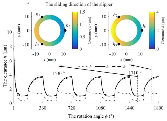
Figure 14. Variation curve of three-point clearance during operation at 300 rpm.

When the cylinder block angle is within the range of 1440–1450°, the slipper traverses the low-pressure to high-pressure transition zone. During this interval, the clamping force and the forward tilting torque exerted by the piston ball head increase rapidly. However, the oil film beneath the slipper in this region is relatively thick, leading to a weaker wedge hydrodynamic effect. To counterbalance the swiftly rising clamping force from the piston, the slipper must shift downward as a whole to apply compressive pressure and augment the hydrodynamic effect. Meanwhile, to offset the increased forward tilting torque, the slipper needs to alter the pressure distribution to create a counteracting torque against the forward tilt by tilting forward. This dynamic is reflected in the figure by a rapid decrease in the clearances of the bearing land, with h₂ and h₃ reducing at a faster rate compared to h₁.

When the cylinder block angle is within the range of 1450–1530°, as the slipper moves through the front of the high-pressure zone, it continues to provide the necessary compressive force to balance the piston clamping force in accordance with the residual clamping force design principle. However, as the oil film thins, the wedge hydrodynamic effect strengthens, and the stiffness of the system increases, resulting in a decrease in the rate at which the clearances of bearing land are reduced.

When the cylinder block angle is within the range of 1530–1610°, as the slipper progresses through the back of the high-pressure zone, the frictional torque from the piston ball head transitions from a forward tilting torque to a backward tilting torque, which gradually increases. During this interval, a slight increase in the clearances h₂ and h₃ of the slipper’s bearing land can be observed, while the clearance h₁ shows a conspicuous decrease.

When the cylinder block angle is within the range of 1610–1626°, as the slipper crosses the high-pressure to low-pressure transition zone, the clamping force from the piston gradually decreases to the casing pressure, and the elasticity on the bearing land recovers, leading to a rapid increase in the clearances at the three points along the outer edge of the slipper’s bearing land.

When the cylinder block angle is within the range of 1626–1800°, as the slipper travels through the low-pressure zone, the frictional torque from the piston ball head gradually shifts from backward tilting torque to forward tilting torque. This transition is depicted in the figure by a slowdown in the rate of increase for the clearance curves h₂ and h₃, and a deceleration in the rate of decrease for the clearance curve h₁.

Under low-speed conditions, the variation in the minimum clearance of the slipper bearing land as the cylinder block’s rotation angle is depicted in Figure 15. Throughout the entire operational cycle, the figure illustrates that the minimum clearance of the bearing land is less than three times the RMS roughness (indicated by the dashed line in the figure). It can be inferred that the bearing land is in a mixed lubrication state and will experience contact wear. The minimum clearance changes on the slipper bearing land during one operating cycle with a cylinder block angle of 1440–1800° are as follows.

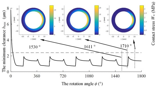
Figure 15. Curve of minimum bottom clearance variation with cylinder block rotation angle during operation at 300 rpm.

When the cylinder block angle is within the range of 1440–1450°, as the slipper traverses the low-pressure to high-pressure transition zone, the high-pressure oil from the piston chamber causes the bearing land to deform under pressure, leading to a rapid increase in the minimum clearance. When the cylinder block angle is within the range of 1450–1610°, as the slipper is passing through the high-pressure zone, it continuously descends to compress the oil film to balance the remaining clamping force. Consequently, the curve of the minimum clearance of the bearing land gradually declines as the cylinder block rotates. When the cylinder block angle is within the range of 1610–1626°, as the slipper crosses the high-pressure to low-pressure transition zone, the expansion of the piston chamber volume and the sudden drop in pressure allow the elasticity on the bearing land to recover. During this recovery, a large elastic contact force will be generated, causing a rapid bounce-back at the contact end. Thus, in this segment, the minimum clearance curve of the slipper’s bearing land first rapidly decreases and then rapidly rises. When the cylinder block angle is within the range of 1626–1800°, as the slipper moves through the low-pressure region, it primarily bears the clamping force from the central spring that restrains the slipper from detaching from the swashplate. Given the sliding speed of the slipper is not high and the dynamic pressure effect is not strong, the curve of the minimum clearance does not elevate further.

Three instances are particularly representative: when the cylinder block angle is 1530°, the slipper is in the middle of the high-pressure zone. at 1612°, the slipper experiences the maximum metal deformation. and at 1710°, the slipper slips through the middle of the low-pressure zone. When the cylinder block angle reaches 1530°, the contact area on the bearing land is located at the trailing edge of the sliding path, with a large contact area and a relatively uniform stress distribution. The maximum contact stress is approximately 17.8 MPa. When the cylinder block angle reaches 1611°, the contact region on the bottom of the bearing land is similarly situated at the trailing edge, but with a higher maximum contact stress of about 21.7 MPa. When the cylinder block angle reaches 1710°, the contact area on the bearing land has shrunk, and the maximum contact stress has decreased to around 3.4 MPa.

5.3. Wear on the Bottom of Slipper Under High-Speed Conditions

In this section, the rotational speed of the cylinder block is set at 3000 rpm, under high-speed conditions, the clearance curves for the three reference points along the outer edge of the slipper’s bearing land are depicted in Figure 16. The clearance curves for these three points stabilize after a cylinder block rotation angle of 720°. Notably, the clearance value h₃ at point A₃ is the smallest among the three reference points, indicating that the slipper presents an inward tilt posture. To illustrate this, we will use the example of a single operating cycle from 1440° to 1800°.

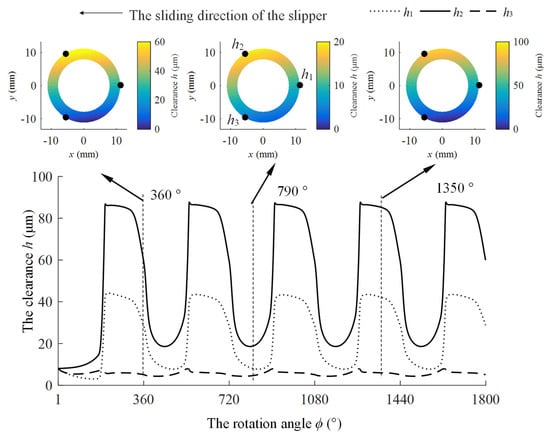
Figure 16. Variation curve of three-point clearance during operation at 3000 rpm.

When the cylinder block angle is within the range of 1440–1450°, the slipper traverses the low-pressure to high-pressure transition zone. During this interval, the clamping force and the forward tilting torque from the piston ball head increase rapidly. However, the oil film beneath the slipper’s bearing land in this region is relatively thick, leading to a weaker wedge hydrodynamic effect. To counterbalance the swiftly rising clamping force from the piston, the slipper must shift downward as a whole to apply compressive pressure and augment the hydrodynamic effect. Meanwhile, to offset the increased forward tilting torque, the slipper needs to alter the pressure distribution to create a counteracting torque against the forward tilt. This dynamic is reflected in the figure by a rapid decrease in the clearances of the bearing land, with h₂ reducing at a faster rate compared to h₁.

When the cylinder block angle is within the range of 1450–1530°, as the slipper moves through the front of the high-pressure zone, the forward tilting torque from the piston ball head decreases. Under the residual clamping force design principle, the slipper still needs to provide compressive force to balance the piston clamping force. However, as the oil film thins, the wedge hydrodynamic effect strengthens, and the stiffness of the system increases. This is reflected in the figure by a reduction in the rate at which the clearances h₁ and h₂ of the slipper’s bearing land decrease.

When the cylinder block angle is within the range of 1530–1610°, with the slipper progressing through the back of the high-pressure zone, the frictional torque from the piston ball head transitions from a forward tilting torque to a backward tilting torque, which gradually increases. In the figure, there is a continued decrease in the clearance h₁ of the bearing land, whereas the clearances h₂ and h₃ show some increment.

When the cylinder block angle is within the range of 1610–1626°, as the slipper crosses the high-pressure to low-pressure transition zone, the clamping force from the piston gradually decreases to the casing pressure, and the elasticity on the bearing land recovers. The figure shows that the clearance h₁, h₂, and h₃ of the slipper’s bearing land increases rapidly. Differing from low-speed conditions, the hydrodynamic effect is stronger under high-speed conditions, resulting in a more pronounced increase in these clearances. By the cylinder block rotation angle of 1633°, the clearance exceeds the maximum limiting film thickness h_c, indicating a collision between the slipper and the retainer.

When the cylinder block angle is within the range of 1633–1800°, as the slipper travels through the low-pressure zone, the frictional torque from the piston ball head gradually shifts from backward tilting torque to forward tilting torque. This transition is depicted in the figure by a decline in the h₂ and h₃ clearance curves, with their rate of decrease becoming more pronounced, while the h₁ clearance curve exhibits a relatively smoother change.

Under high-speed conditions, the variation in the minimum clearance of the bearing land as the cylinder block’s rotation angle is depicted in Figure 17. Specifically, this illustration presents the minimum clearance changes on the slipper bearing land during one operating cycle with a cylinder block angle of 1440–1800°.

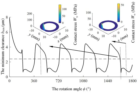
Figure 17. Curve of minimum clearance variation with cylinder block rotation angle during operation at 3000 rpm.

When the cylinder block angle is within the range of 1440–1450°, as the slipper passes through the transition from low-pressure to high-pressure, the high-pressure oil from the piston chamber causes the bearing land to deform under pressure, leading to a rapid increase in the minimum clearance. When the cylinder block angle is within the range of 1450–1475°, the slipper is sliding through the high-pressure zone. On the one hand, the increase in clamping force causes the slipper to move downwards as a whole, and on the other hand, the enhanced flow of differential pressure improves the tilting situation of the slipper. Therefore, the minimum clearance between the bottom of the slipper bearing land increases in this range.

When the cylinder block angle is within the range of 1475–1610°, the slipper is traversing the high-pressure zone. Here, the slipper must continuously descend and compress the oil film to counterbalance the residual clamping force. Consequently, the curve of the minimum clearance of the slipper’s bearing land decreases as the cylinder block rotates. When the cylinder block angle is within the range of 1610–1626°, the slipper transitions through the high-pressure to low-pressure zone, the motion of the slipper become intricate. On one hand, the increase in the piston chamber volume and the sudden drop in pressure allow for the elastic recovery of the slipper’s bearing land. Simultaneously, under the action of hydrodynamic lubrication pressure, the slipper tends to lift rapidly. Following this uplift, as the oil film thickens, its resistance against tilting diminishes, causing the slipper to incline rapidly towards the inner side. Considering these factors collectively, the trend in the curve of the minimum clearance of the slipper’s bearing land during this period shows a decline.

When the cylinder block angle is 1633°, the collision between the slipper and the retainer occurs, marking the minimum clearance curve of the slipper’s bearing land no longer decreases. When the cylinder block angle is within the range of 1633–1800°, with the slipper slips through the low-pressure zone, its operation at high-speed leads to an inward tilt that is not conducive to forming an effective wedge-shaped converging clearance. Consequently, the increase in the curve of the minimum clearance of the slipper’s bearing land is limited.

The figure illustrates that at a cylinder block angle of 1620°, the minimum clearance of the bearing land is lower than three times the RMS of roughness (indicated by the dashed line in the figure). When the cylinder block angle reaches 1633°, the minimum clearance of the slipper’s bearing land reaches its lowest value, indicating there is a significant metal contact deformation between the slipper and the swashplate. The contact area is localized on the inner side of the slipper’s revolution, with the maximum contact pressure reaching approximately 168 MPa. When the cylinder block angle is 1710°, the maximum contact pressure is approximately 53.7 MPa.

In this section, the micro-motion of the slipper and wear characteristics of the slipper’s bearing land were studied and analyzed under three typical operating conditions. Regardless of whether the slipper has an ideally flat bottom or operates under low-speed or high-speed conditions, achieving both force and torque balance within fluid lubrication conditions proves challenging, which may lead to contact wear between the bearing land and the swashplate. Regarding the position of contact wear, the contact wear of the slipper with the ideal flat bottom occurs at the sliding front end. In low-speed conditions, the contact wear of the slipper occurs at the sliding back end. Conversely, under high-speed conditions, the wear is concentrated on the inner side of the slipper’s revolution sliding. From the perspective of contact stress and contact area, the contact area between the ideal flat bottom slipper and the swashplate is larger under low-speed conditions, and the contact stress is relatively smaller. Under high-speed conditions, the contact area between the slipper and the swashplate is small, but the contact stress is high, resulting in eccentric wear.

6. Conclusions

(1)

A method has been proposed to predict the instantaneous uneven wear of the slipper bearing land using the Archard dry friction wear formula. Specifically, by employing the G-W roughness model and Hertz contact theory, the metallic contact stress between the slipper and swashplate is calculated and substituted into the Archard dry friction wear formula, which can directly solve and predict the instantaneous uneven wear of the bearing land under different lubrication conditions.

(2)

The contact wear characteristics under extreme conditions have been explored, which elucidated the patterns of wear location and contact stress variations for the slipper in three typical operating conditions: ideal flat-bottomed, low-speed, and high-speed. Regarding the position of contact wear, the contact wear on the ideal flat-bottomed slipper occurs at the leading edge of the sliding: at low-speed, it occurs at the trailing edge of the sliding; and at high-speed, it occurs on the inner side of the revolution. In terms of contact stress and contact area, the ideal flat-bottomed slipper and those in low-speed conditions display larger contact areas and lower contact stresses. Conversely, under high-speed conditions, the contact area is smaller, but the contact stress is higher, manifesting as uneven wear.

(3)

After running, the wear depth and oil film thickness of the slipper bottom are of the same order of magnitude. In a mixed lubrication state, these parameters are sensitive factors that determine the lubrication performance of the slipper.

References

- Yin, F.L.; Chen, Y.T.; Ma, Z.H.; Nie, S.L.; Ji, H. Investigation on mixed thermalelstohydrodynamic lubrication behavior of slipper/swashplate interface in water hydraulic axial piston pump. Tribol. Int. 2023, 189, 108896. [Google Scholar] [CrossRef]
- Liu, S.Y.; Yu, C.S.; Ai, C.; Zhang, W.Z.; Li, Z.; Zhang, Y.Q.; Jiang, W.L. Impact Analysis of worn surface morphology on adaptive friction characteristics of the slipper pair in hydraulic pump. Micromachines 2023, 14, 682. [Google Scholar] [CrossRef]
- Guo, M.; Nie, S.L.; Ji, H.; Yin, F.L. Design and lubrication characteristics of a new integrated slipper/swashplate interface in seawater hydraulic piston. China Mech. Eng. 2022, 33, 2942–2952. [Google Scholar] [CrossRef]
- Mo, H.; Hu, Y.P.; Quan, S. Thermo-hydrodynamic lubrication analysis of slipper pair considering worn profile. Lubricants 2023, 11, 190. [Google Scholar] [CrossRef]
- Zhang, C.C.; Zhu, C.H.; Meng, B.; Li, S. Challenges and solutions for High-Speed aviation piston pumps: A review. Aerospace 2021, 8, 392. [Google Scholar] [CrossRef]
- Ni, S.L.; Wu, H.C.; Zhao, L.M.; Yang, L. Study on the effect of material matching to the performance of dry friction of the slipper pair in axial piston pump under high pressure. Mach. Des. Manuf. 2019, 3, 12–15. [Google Scholar] [CrossRef]
- Li, Y.; He, Y.; Luo, J. Surface modifications and performance enhancements of key friction pairs in aviation hydraulic piston pumps. J. Tsinghua Univ. (Sci. Technol.) 2021, 61, 1405–1422. [Google Scholar] [CrossRef]
- Li, S.N.; Yang, P.; Bao, S.L.; Li, Y. Numerical simulation of fluid-structure-thermal coupling of slipper pair in high-pressure and large-displacement radial piston pump. J. Drain. Irrig. Mach. Eng. 2022, 40, 887–894. [Google Scholar]
- Schenk, A.; Ivantysynova, M. A transient thermoelastohydrodynamic lubrication model for the slipper/swashplate in axial piston machines. J. Tribol. 2015, 137, 031701. [Google Scholar] [CrossRef]
- Zuo, X. Fractal Characterization of Worn Surface Topography and Its Variation During Wear Process. Ph.D. Thesis, China University of Mining and Technology, Beijing, China, 2017. [Google Scholar]
- Li, Z.A. Study on the Influence Mechanism of Worn Surface Morphology Evolution Process on Slipper Pair Lubrication Performance. Master’s Thesis, Yanshan University, Qinhuangdao, China, 2023. [Google Scholar]
- Bergada, J.M.; Watton, J.; Haynes, J.M.; Davies, D.L. The hydrostatic/hydrodynamic behaviour of an axial piston pump slipper with multiple lands. Meccanica 2010, 45, 585–602. [Google Scholar] [CrossRef]
- Spencer, N. Design and Development of a Novel Test Method to Measure the Slipper/Swashplate Interface Fluid Film in a Positive Displacement Machine. Master’s Thesis, Purdue University, West Lafayette, IN, USA, 2014; pp. 93–96. [Google Scholar]
- Fisher, M.J. A Theoretical Determination of Some Characteristics of a Tilted Hydrostatic Slipper Bearing; British Hydromechanics Research Association: Cranfield, UK, 1962. [Google Scholar]
- Harris, R.M.; Edge, K.A.; Tilley, D.G. Predicting the behavior of slipper pads in swashplate-type axial piston pumps. J. Dyn. Sys. Meas. Control 1996, 3, 41–47. [Google Scholar] [CrossRef]
- Hooke, C.J.; Kakoullis, Y.P. The effects of centrifugal load and ball friction on the lubrication of slippers in axial piston pumps. In Proceedings of the Sixth International Fluid Power Symposium, Qingdao, China, 24–27 July 1981; pp. 179–191. [Google Scholar]
- Hooke, C.J.; Li, K.Y. The lubrication of slippers in axial piston pumps and motors-the effect of tilting couples. Proc. Inst. Mech. Eng. Part C J. Mech. Eng. Sci. 1989, 203, 343–350. [Google Scholar] [CrossRef]
- Koc, E.; Hooke, C.J. Considerations in the design of partially hydrostatic slipper bearings. Tribol. Int. 1997, 30, 815–823. [Google Scholar] [CrossRef]
- Xu, B.; Wang, Q.N.; Zhang, J.H. Effect of case drain pressure on slipper/swashplate pair within axial piston pump. J. Zhejiang Univ.-Sci. A 2015, 16, 1001–1014. [Google Scholar] [CrossRef]
- Chao, Q.; Zhang, J.H.; Xu, B.; Wang, Q.N. Discussion on the Reynolds equation for the slipper bearing modeling in axial piston pumps. Tribol. Int. 2018, 118, 140–147. [Google Scholar] [CrossRef]
- Wohlers, A.; Morrenhoff, H. Tribological simulation of hydrostatic swash plate bearing in an axial piston pump. In Proceedings of the Power Transmission and Motion Control Symposium, Bath, UK, 12–14 September 2007; pp. 129–144. [Google Scholar]
- Canbulut, F. The experimental analyses of the effects of the geometric and working parameters on the circular hydrostatic thrust bearings. JSME Int. J. Ser. C Mech. Syst. Mach. Elem. Manuf. 2005, 48, 715–722. [Google Scholar] [CrossRef][Green Version]
- Canbulut, F.; Sinanoğlu, C.; Koc, E. Experimental analysis of frictional power loss of hydrostatic slipper bearings. Ind. Lubr. Tribol. 2009, 61, 123–131. [Google Scholar] [CrossRef]
- Ivantysyn, R.; Shorbagy, A.; Weber, J. Investigation of the wear behavior of the slipper in an axial piston pump using simulation and measurement. In Proceedings of the 12th International Fluid Power Conference, Dresden, Germany, 12–14 October 2020; pp. 315–326. [Google Scholar]
- Du, Z.; Zhang, Y.; Lu, W.; Huang, W. Research on prediction methods for eccentric wear of the slipper pair in axial piston pumps and lubrication performance analysis. J. Tribol. 2024, 146, 092201. [Google Scholar] [CrossRef]
- Long, J.Z.; Lu, Y.; Zhang, H.; Qian, X.B.; Zhang, J.H. Life cycle assessment of a slipper/swash plate friction pair based on thermal-fluid-structure lubrication state dynamic recognition. Tribol. Int. 2024, 192, 109256. [Google Scholar] [CrossRef]
- Chao, Q.; Zhang, J.; Xu, B.; Wang, Q. Multi-position measurement of oil film thickness within the slipper bearing in axial piston pumps. Measurement 2018, 122, 66–72. [Google Scholar] [CrossRef]
- Liu, H.; Yuan, S.H.; Jing, C.B.; Zhao, Y.M. Effects of wear profile and elastic deformation on the slipper’s dynamic characteristics. J. Mech. Eng. 2013, 49, 75–83. [Google Scholar] [CrossRef]
- Chao, Q. Derivation of the Reynolds equation in cylindrical coordinates applicable to the slipper/swash plate interface in axial piston pumps. Proc. Inst. Mech. Eng. Part J J. Eng. Tribol. 2020, 235, 798–807. [Google Scholar] [CrossRef]
- Greenwood, J.A.; Williamson, J.B.P. Contact of nominally flat surfaces. Proc. R. Soc. London. Ser. A 1996, 295, 300–319. [Google Scholar]
- Hou, H.J.; Pei, J.X.; Cao, D.X.; Wang, L. Study on mixed elastohydrodynamic lubrication performance of point contact with Non-Gaussian rough surface. Lubr. Sci. 2024, 36, 51–64. [Google Scholar] [CrossRef]
- Pei, J.X.; Han, X.; Tao, Y.R.; Feng, S.Z. Mixed elastohydrodynamic lubrication analysis of line contact with Non-Gaussian surface roughness. Tribol. Int. 2020, 151, 106449. [Google Scholar] [CrossRef]
- Goodman, N.R. Statistical analysis based on a certain multivariate complex gaussian distribution (an introduction). Ann. Math. Stat. 1963, 34, 152–177. Available online: http://www.jstor.org/stable/2991290 (accessed on 6 November 2025). [CrossRef]
- Wan, L.R.; Jiang, J.Y.; Sun, Z.Y.; Niu, H. Analysis of slipper overturning and collision behavior of the axial piston pump based on rigid-flexible coupling. IEEE Access 2023, 11, 94009–94022. [Google Scholar] [CrossRef]
- Xu, B.; Li, Y.B.; Zhang, B.; Zhang, J.H. Numerical simulation of overturning phenomenon of axial piston pump slipper pair. J. Mech. Eng. 2010, 46, 161–168. [Google Scholar] [CrossRef]
- Archard, J.F. Contact and rubbing of flat surfaces. J. Appl. Phys. 1953, 24, 981–988. [Google Scholar] [CrossRef]
- Christensen, H. Elastohydrodynamic theory of spherical bodies in normal approach. J. Lubr. Technol. 1970, 92, 145–153. [Google Scholar] [CrossRef]
- Wieczorek, U.; Ivantysynova, M. CASPAR-A computer aided design tool for axial piston machines. In Proceedings of the Power Transmission Motion and Control International Workshop, Bath, UK, 13–17 October 2000; pp. 113–126. [Google Scholar]
- Zhao, K.P.; Wang, C.L.; He, T.; Luo, G.; Qin, Y.; Fang, S.Y. Theoretical and experimental study on lubrication and friction of slipper pair of valve distribution piston pump based on FVM-TRD coupling method. Tribol. Int. 2024, 194, 109456. [Google Scholar] [CrossRef]
- Tang, H.S.; Ren, Y.; Xiang, J.W. A novel model for predicting thermoelastohydrodynamic lubrication characteristics of slipper pair in axial piston pump. Int. J. Mech. Sci. 2017, 124–125, 109–121. [Google Scholar] [CrossRef]
- Tang, H.S.; Yin, Y.B.; Zhang, Y.; Li, J. Parametric analysis of thermal effect on hydrostatic slipper bearing capacity of axial piston pump. J. Cent. South Univ. 2016, 23, 333–343. [Google Scholar] [CrossRef]
Disclaimer/Publisher’s Note: The statements, opinions and data contained in all publications are solely those of the individual author(s) and contributor(s) and not of MDPI and/or the editor(s). MDPI and/or the editor(s) disclaim responsibility for any injury to people or property resulting from any ideas, methods, instructions or products referred to in the content. |
© 2025 by the authors. Licensee MDPI, Basel, Switzerland. This article is an open access article distributed under the terms and conditions of the Creative Commons Attribution (CC BY) license (https://creativecommons.org/licenses/by/4.0/).