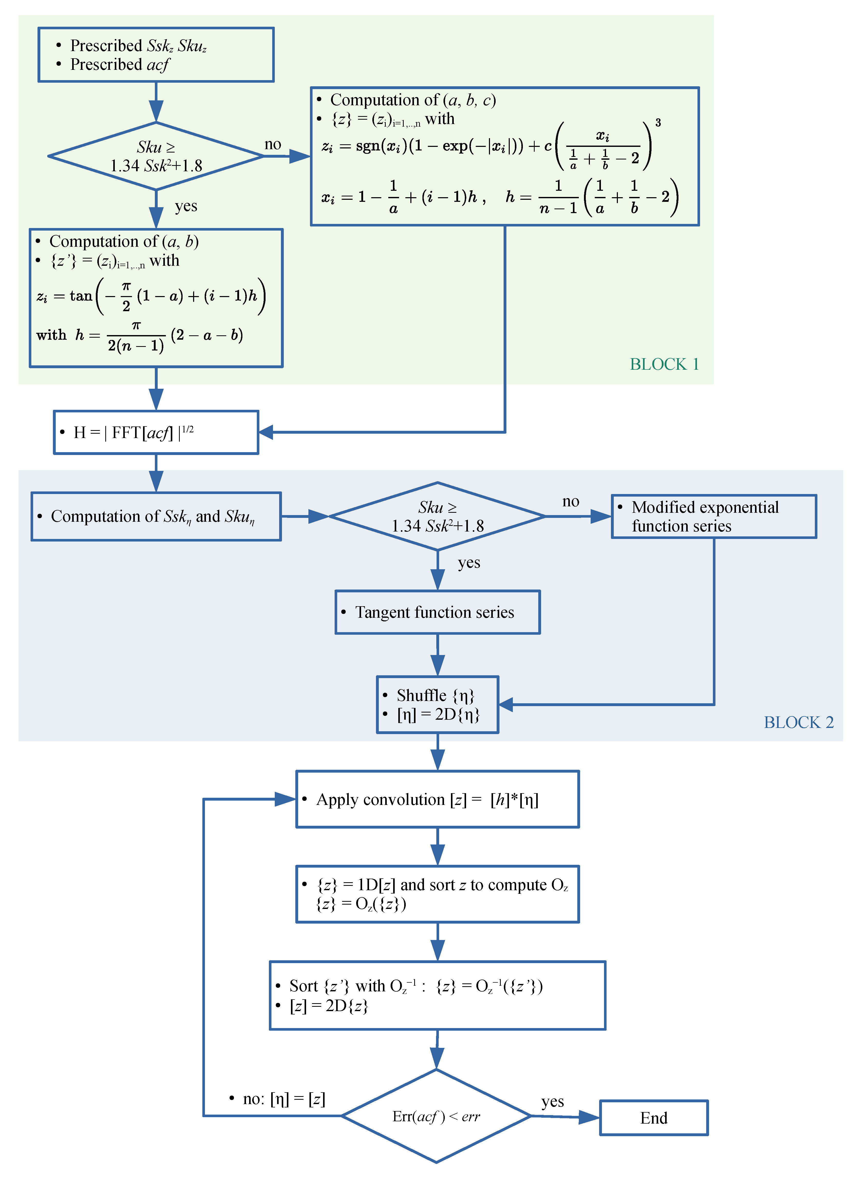
Figure 1.
Flowchart of the modified Hu and Tonder algorithm for rough surface generation. Block 1 can be replaced by the recovery of an existing surface. Block 2 can be replaced by a prescribed texture.
Figure 1.
Flowchart of the modified Hu and Tonder algorithm for rough surface generation. Block 1 can be replaced by the recovery of an existing surface. Block 2 can be replaced by a prescribed texture.
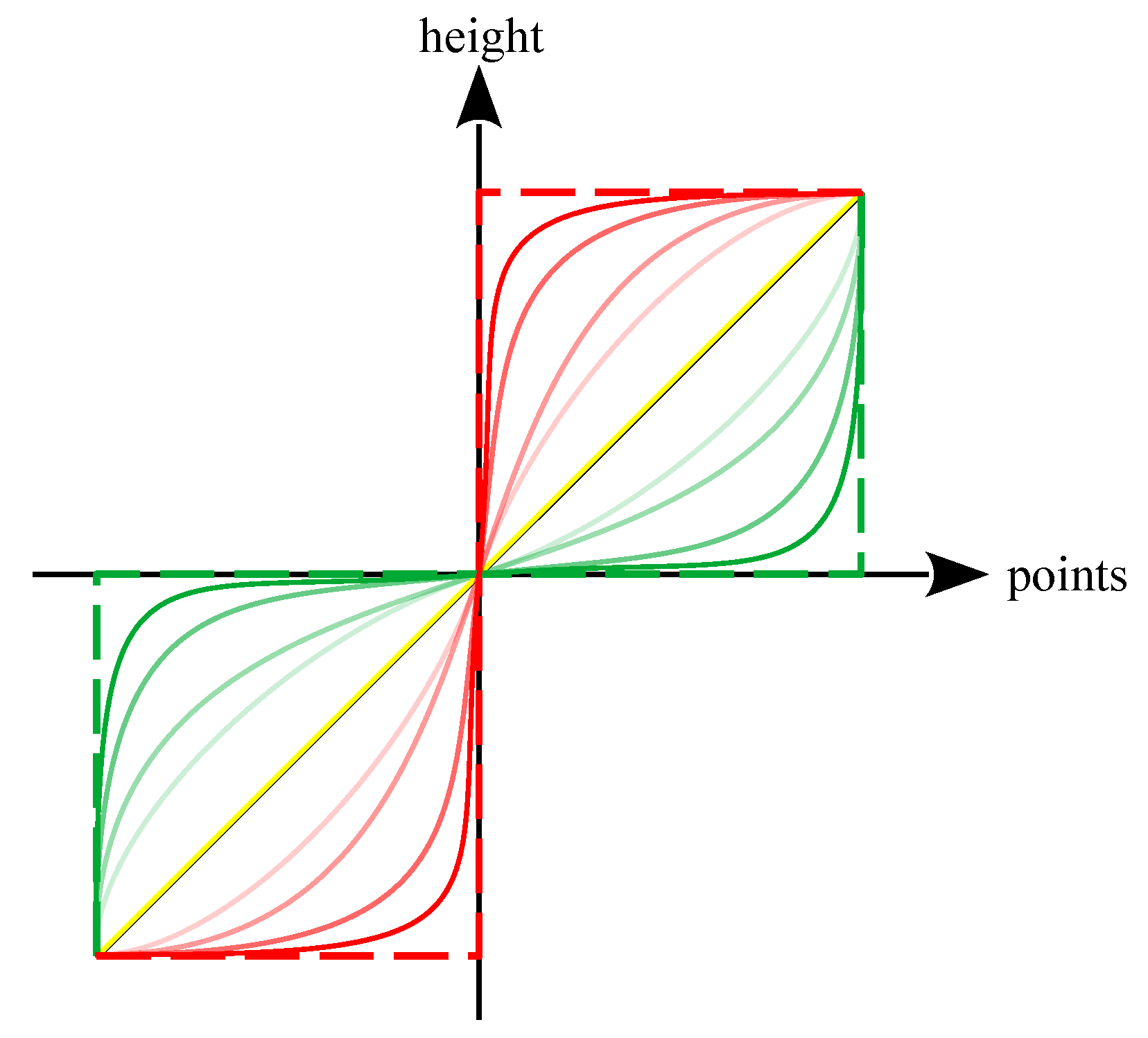
Figure 2.
The principle of a parametric universal function able to cover the whole domain. The red curves may approach the Pearson boundary, whereas the green curves can lead to high values of and .
Figure 2.
The principle of a parametric universal function able to cover the whole domain. The red curves may approach the Pearson boundary, whereas the green curves can lead to high values of and .
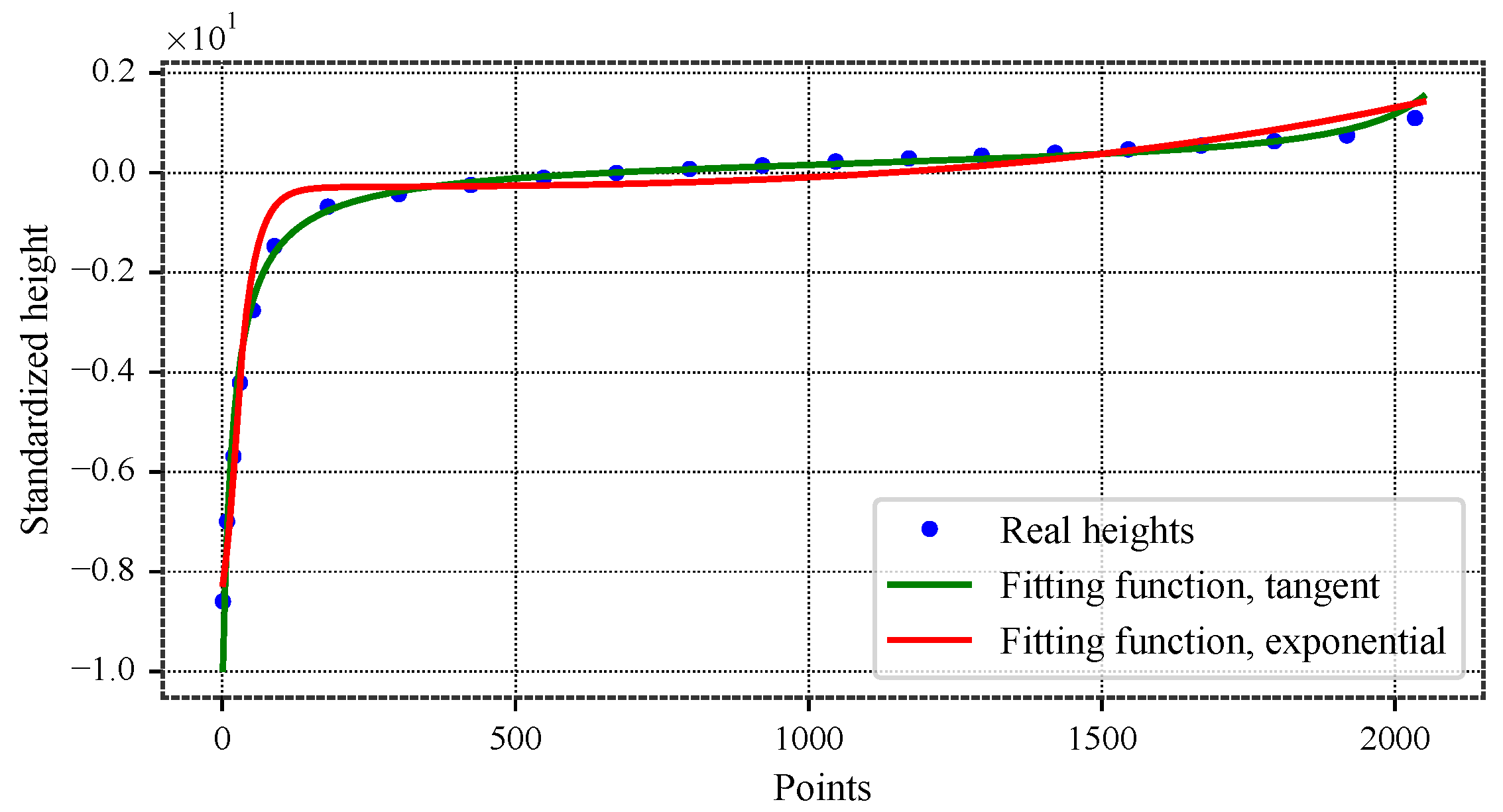
Figure 3.
Best fit of a rotor surface material curve with tangent and modified exponential functions: and . The rotor heights were measured using a white-light interferometric microscope. From the original surface containing approximately one million points, a representative subset of about 2000 points preserving the minima and maxima was retained. The adjusted heights, on the other hand, are generated numerically.
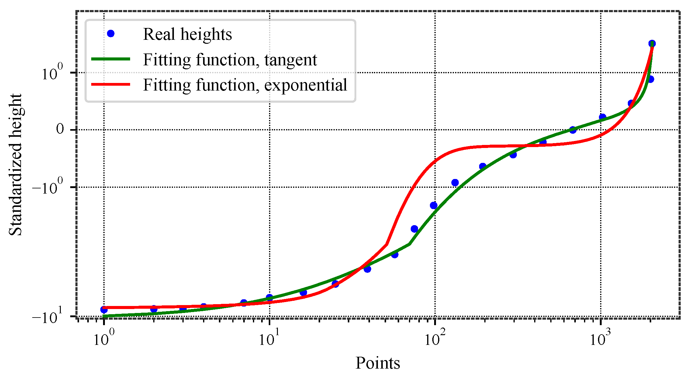
Figure 4.
Best fit of a rotor surface material curve with tangent and modified exponential functions. Logarithmic scale.
Figure 4.
Best fit of a rotor surface material curve with tangent and modified exponential functions. Logarithmic scale.
Figure 5.
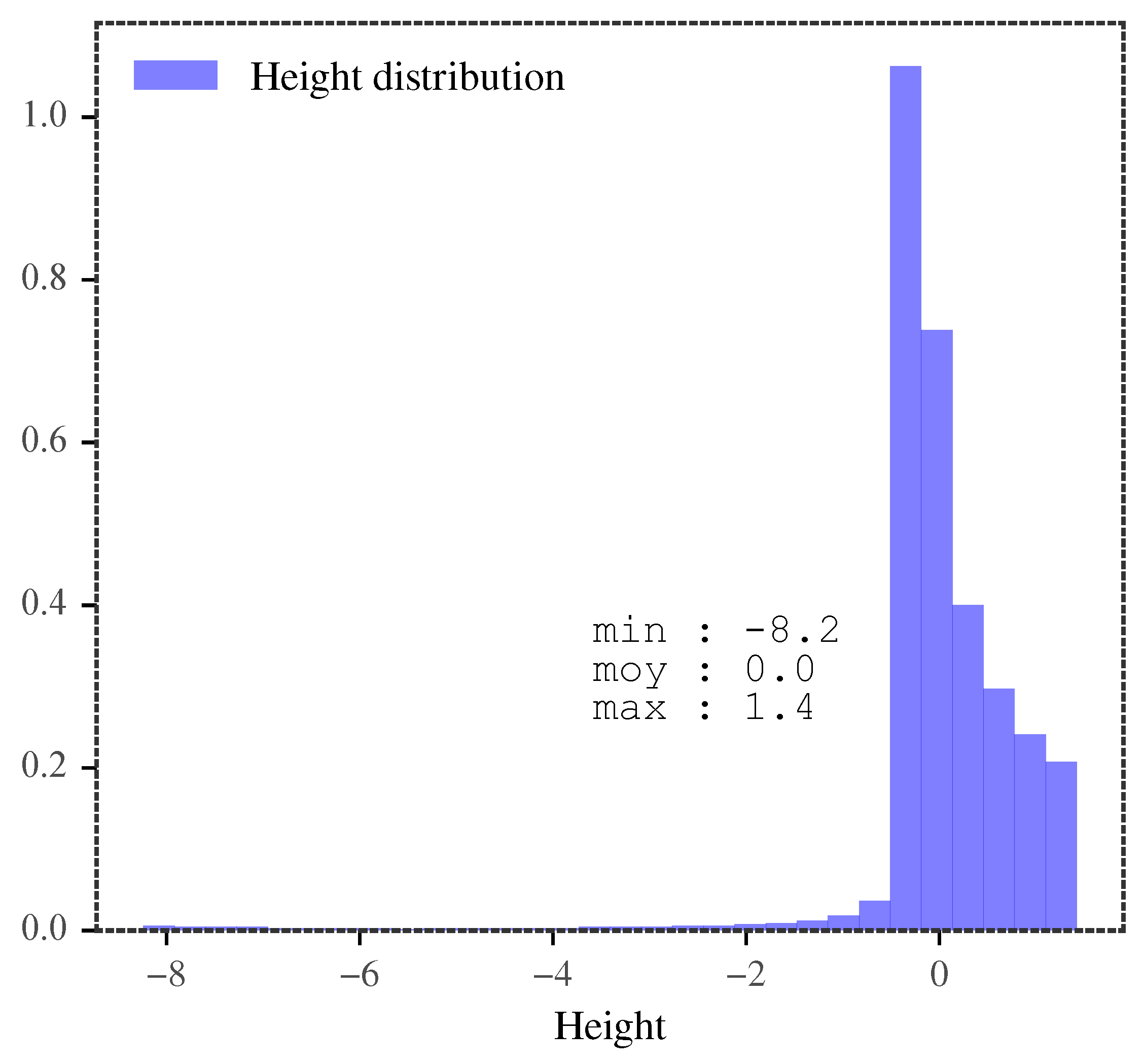
Height histogram of the rotor surface showing unimodality.
Figure 5.
Height histogram of the rotor surface showing unimodality.
Figure 6.
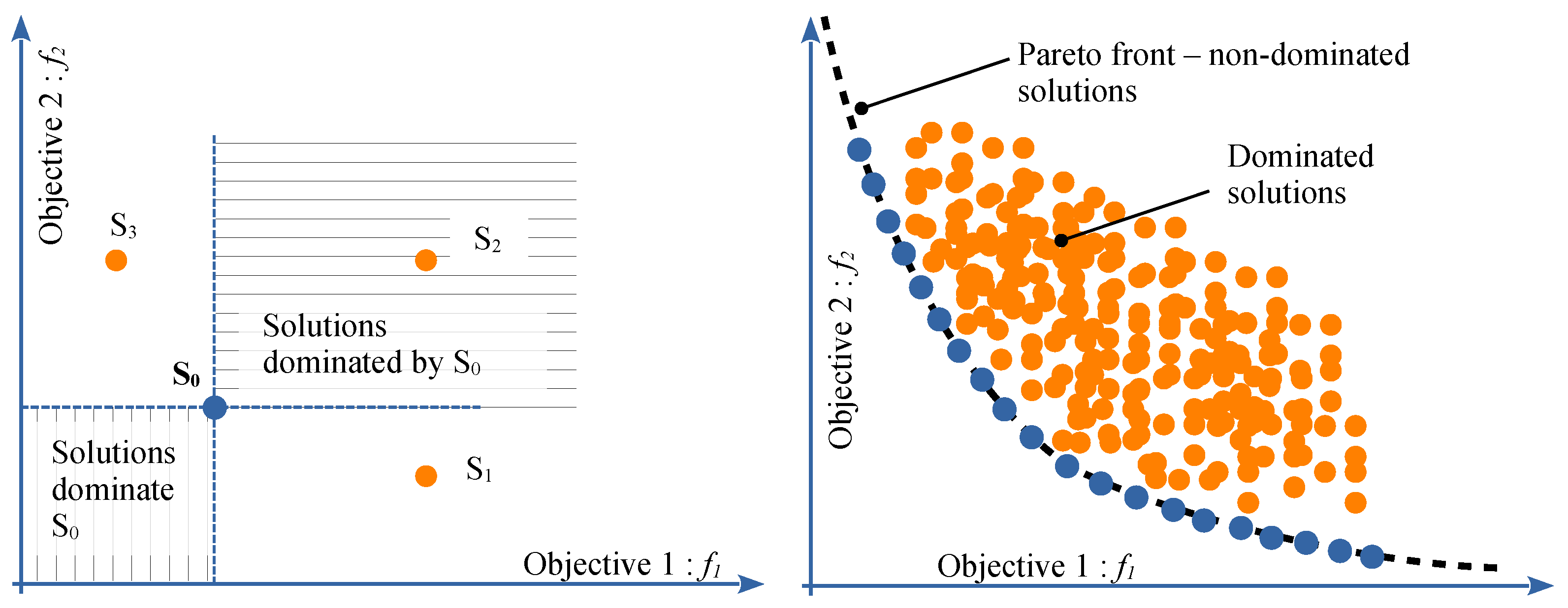
The Pareto front principle.
Figure 6.
The Pareto front principle.
Figure 7.
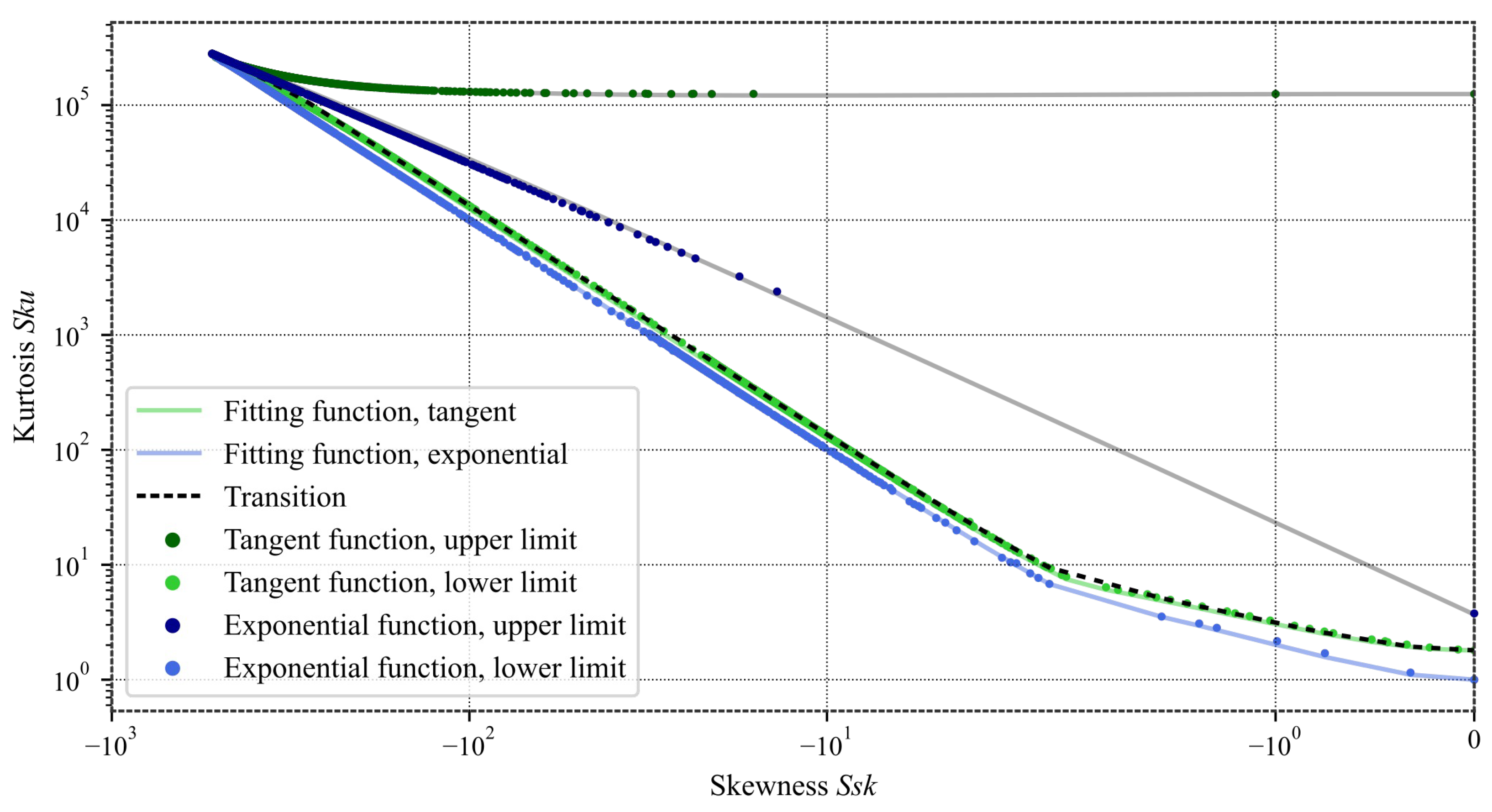
Analytical function boundaries in log scale. Note that for rough surfaces, is most of the time negative. The upper bounds were not fitted, since their analytical form is of no practical significance; the grey lines are only used to delimit the relevant region.
Figure 7.
Analytical function boundaries in log scale. Note that for rough surfaces, is most of the time negative. The upper bounds were not fitted, since their analytical form is of no practical significance; the grey lines are only used to delimit the relevant region.
Figure 8.
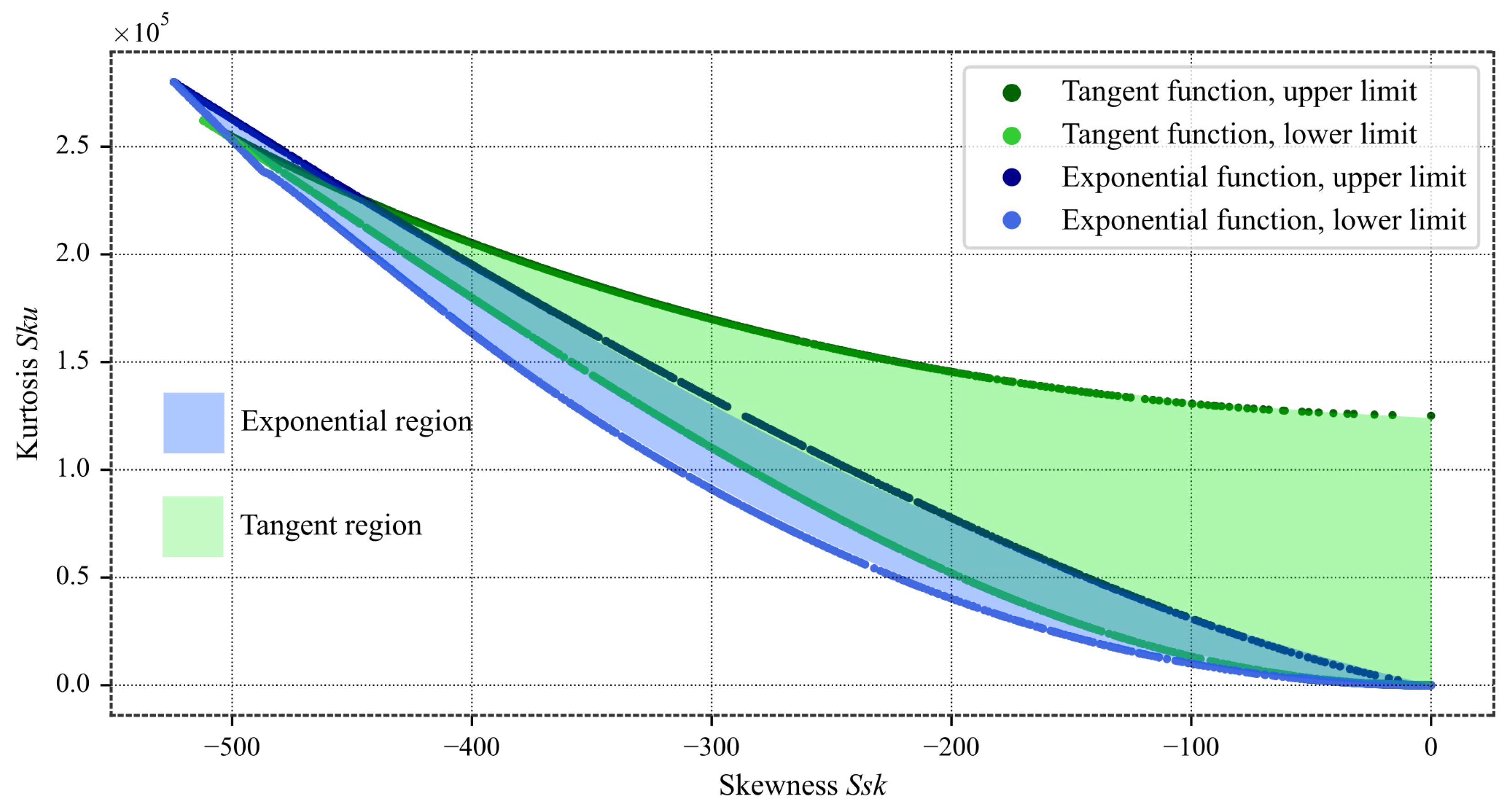
Analytical function boundaries.
Figure 8.
Analytical function boundaries.
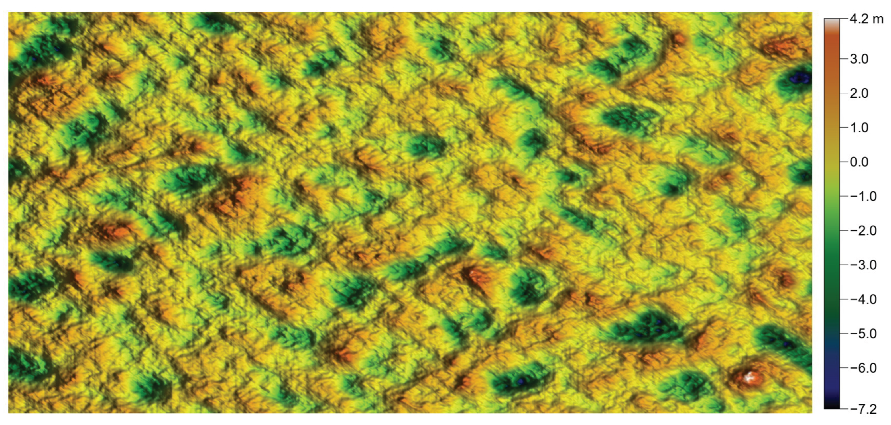
Figure 9.
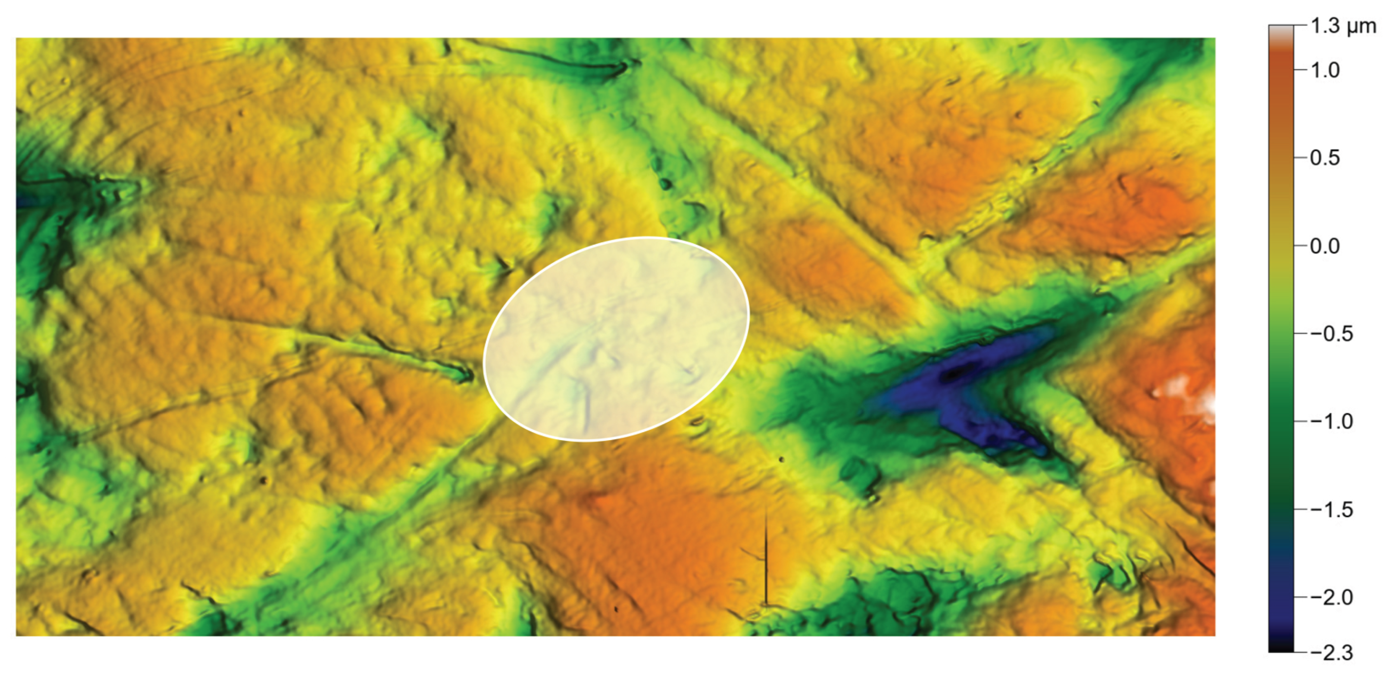
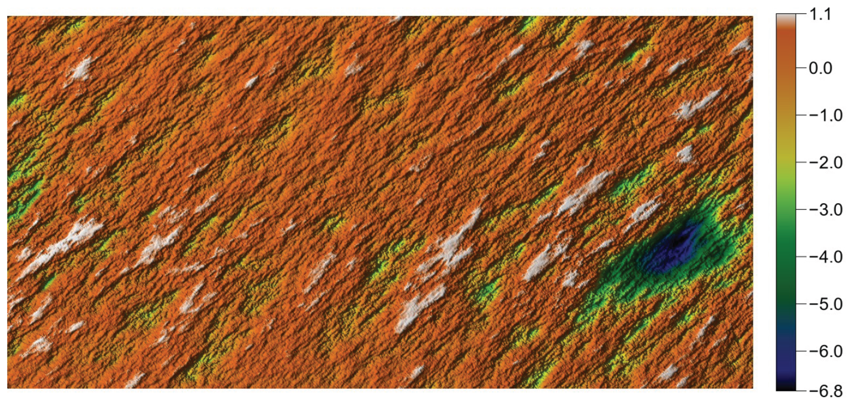
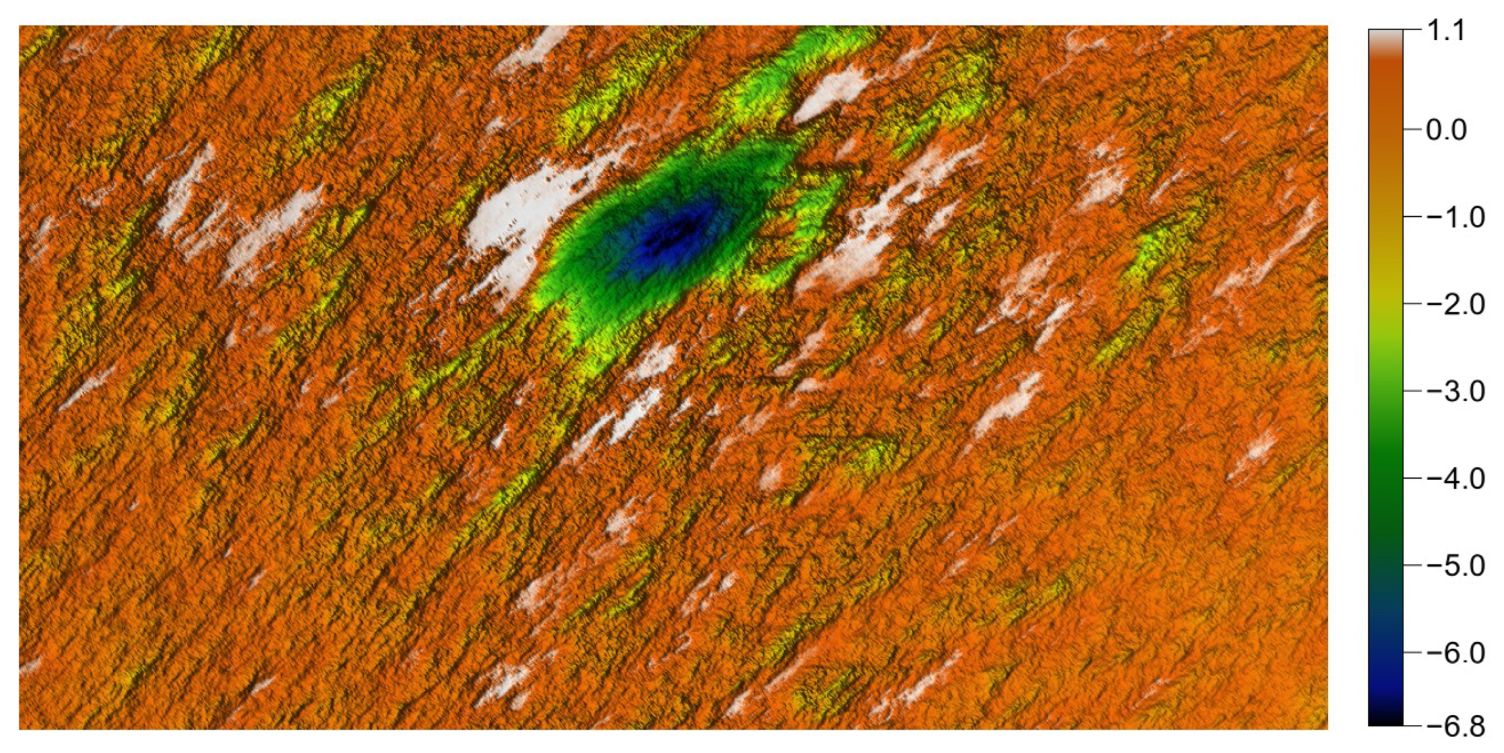
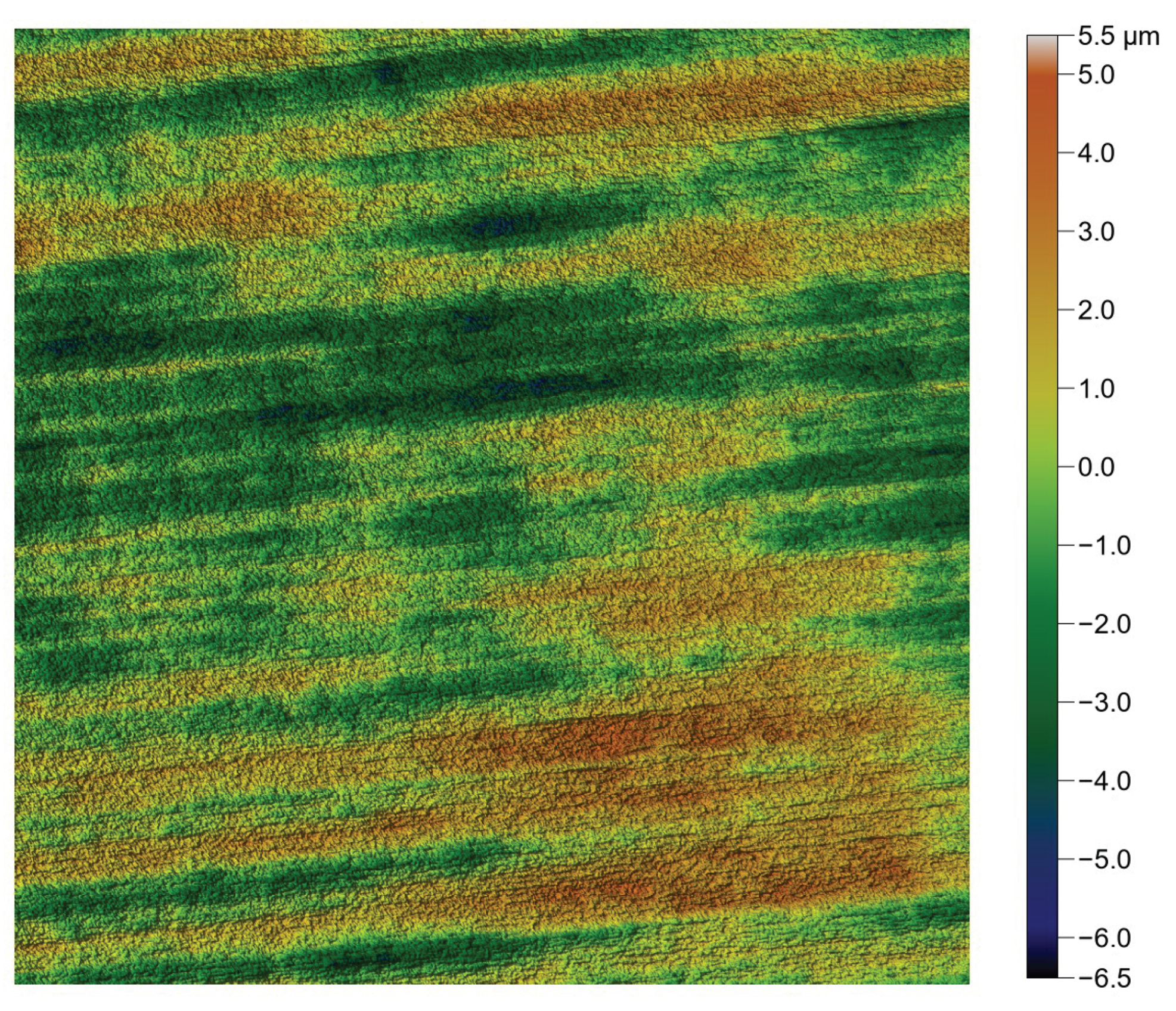
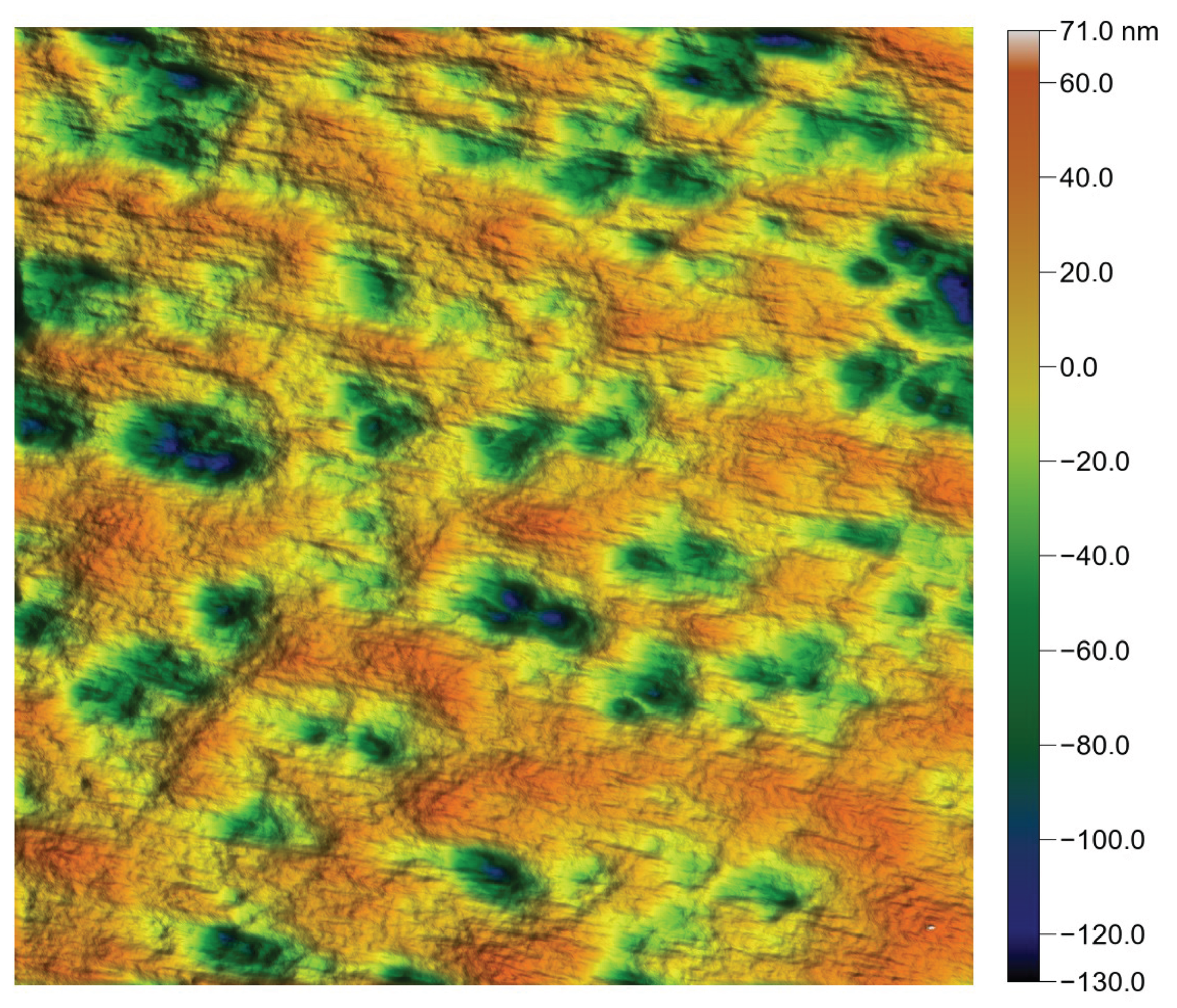
Dental surface of a grazer-type herbivore. 1024 × 512 px surface, size = 132 × 66 m. , , , m. The white ellipsis is the autocorrelation function cut at . Note that stands for .
Figure 9.
Dental surface of a grazer-type herbivore. 1024 × 512 px surface, size = 132 × 66 m. , , , m. The white ellipsis is the autocorrelation function cut at . Note that stands for .
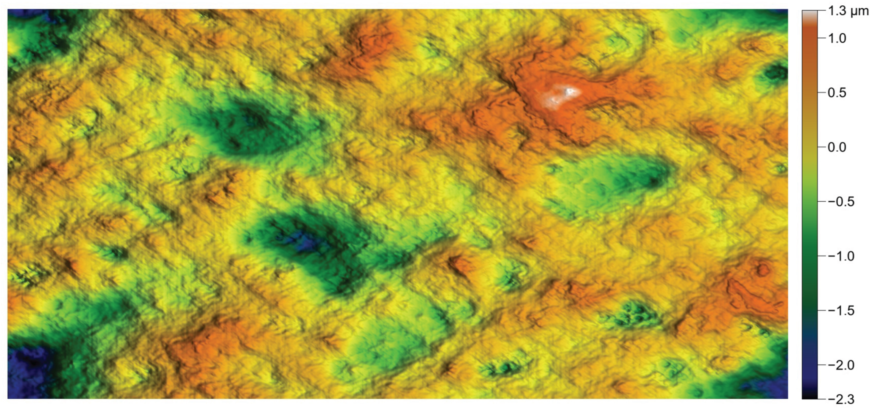
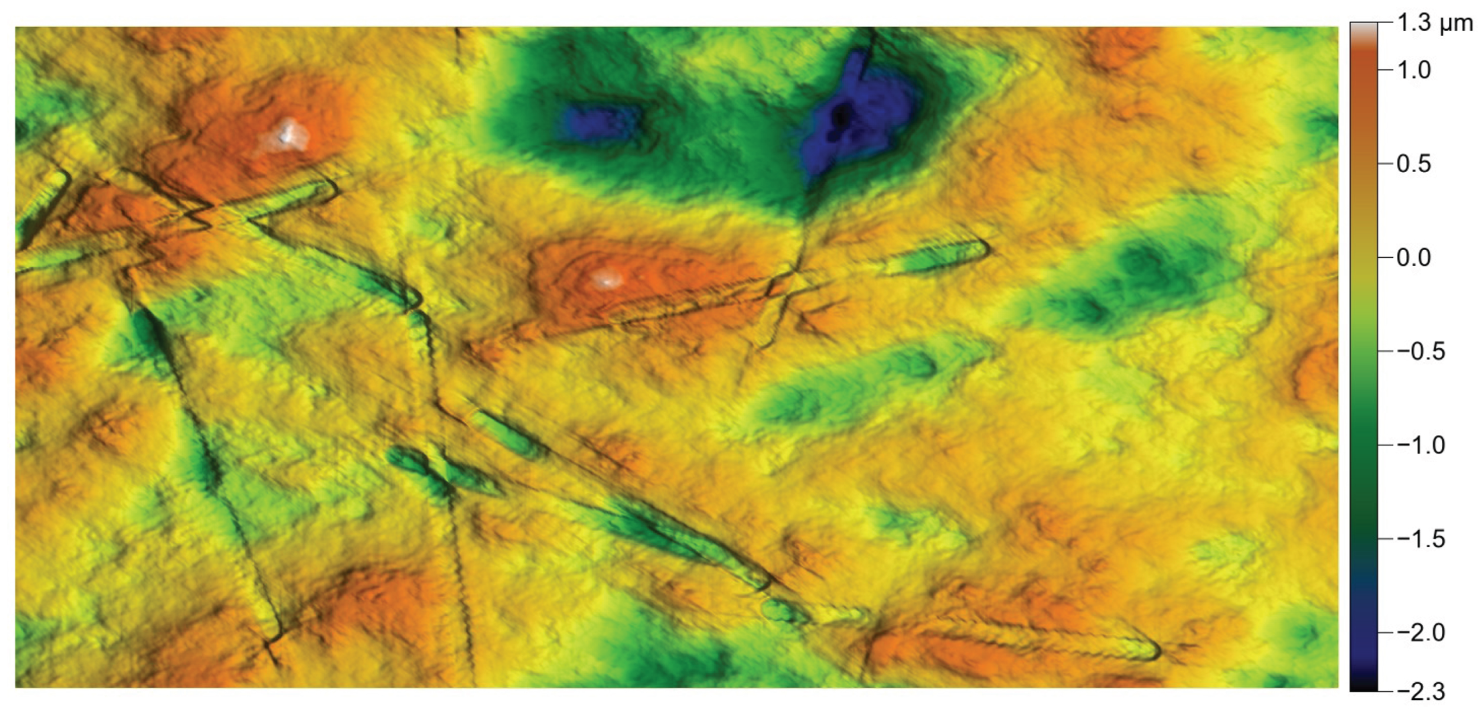
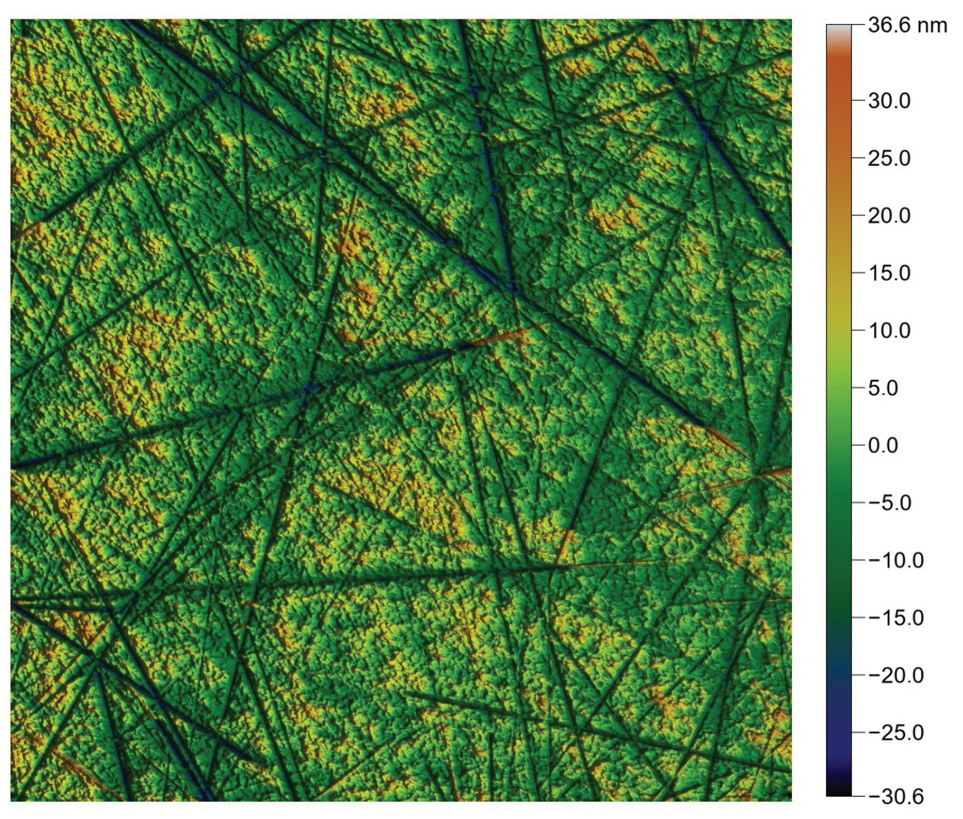
Figure 10.
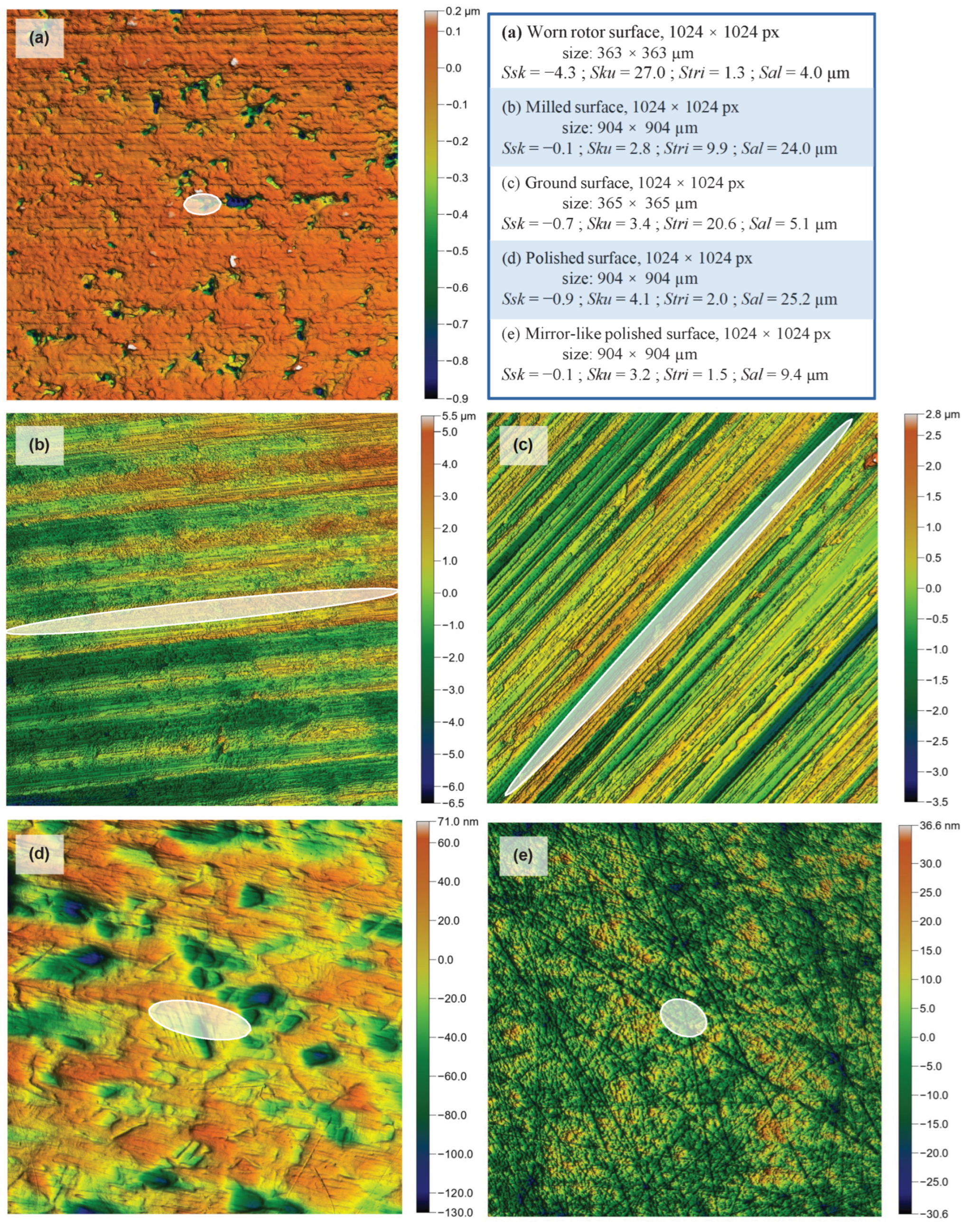
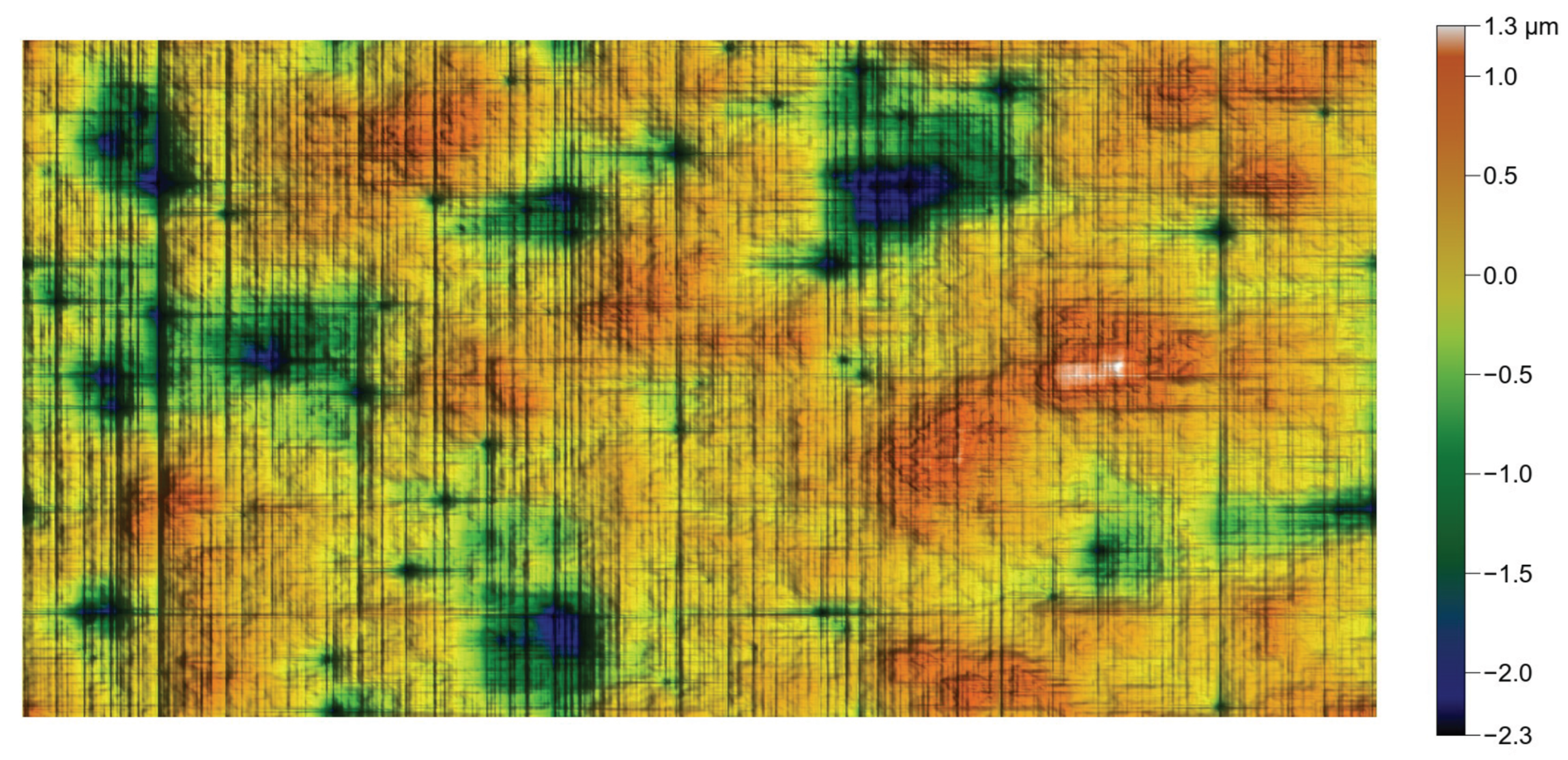
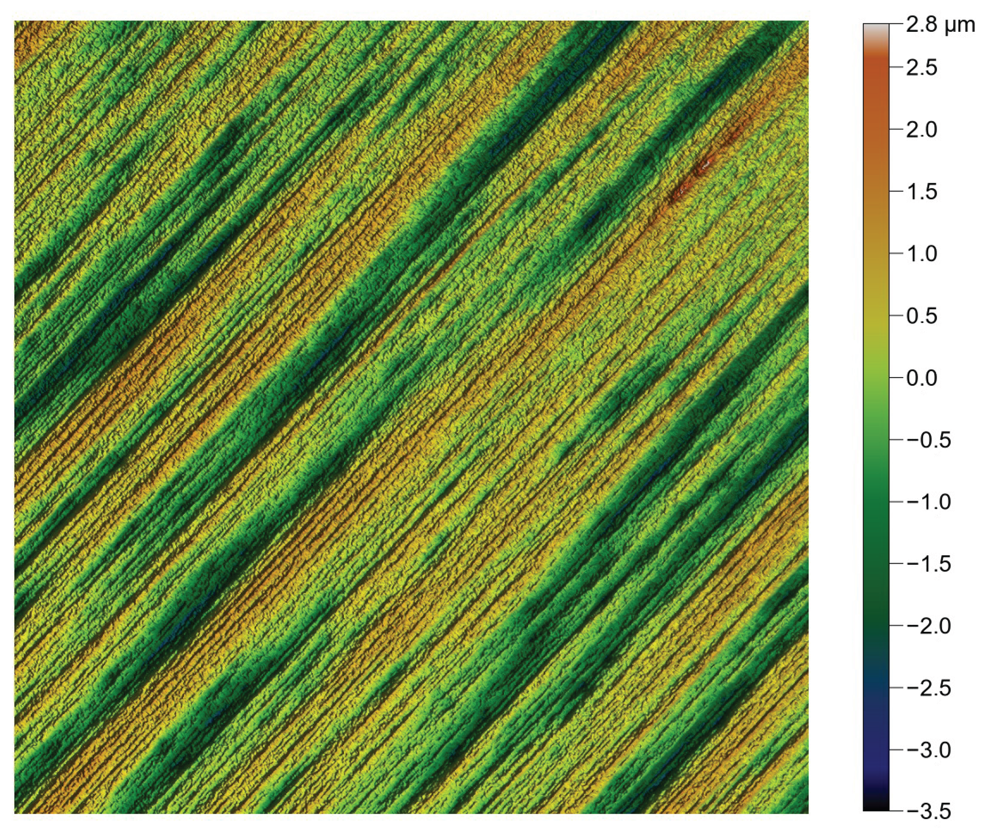
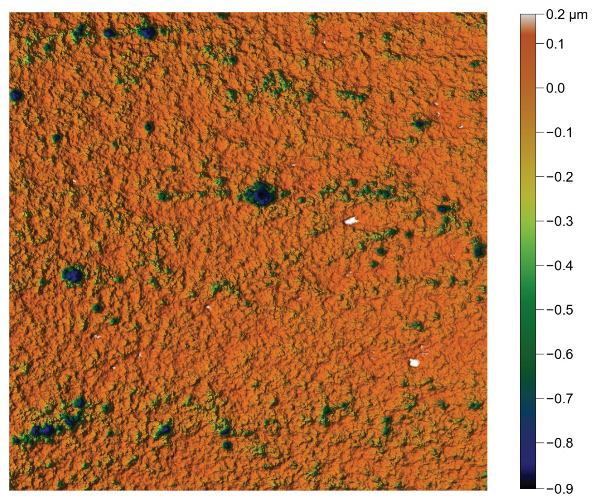
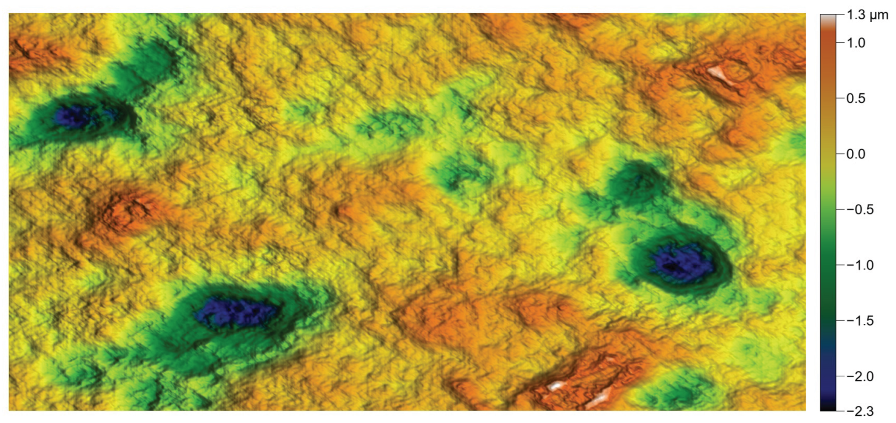
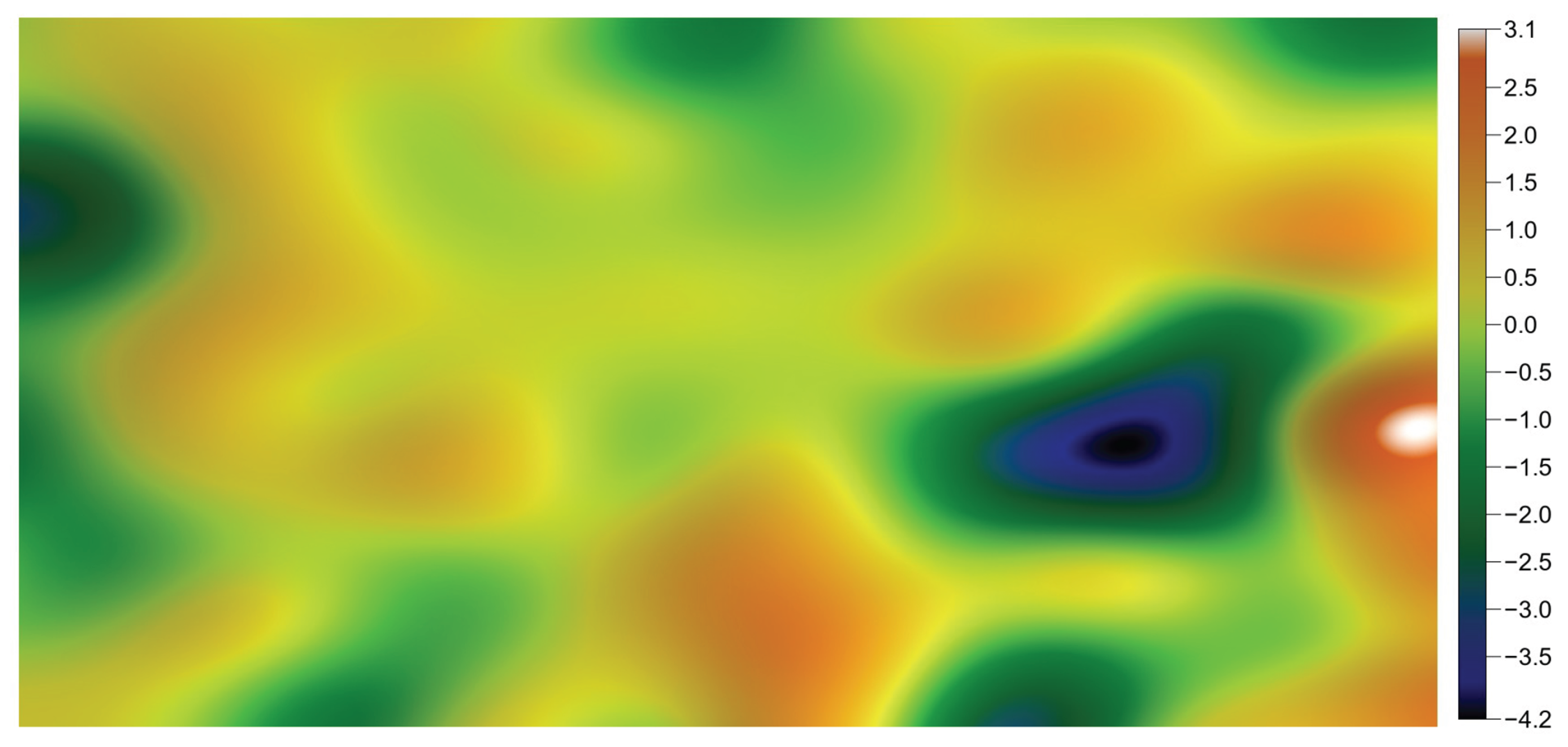
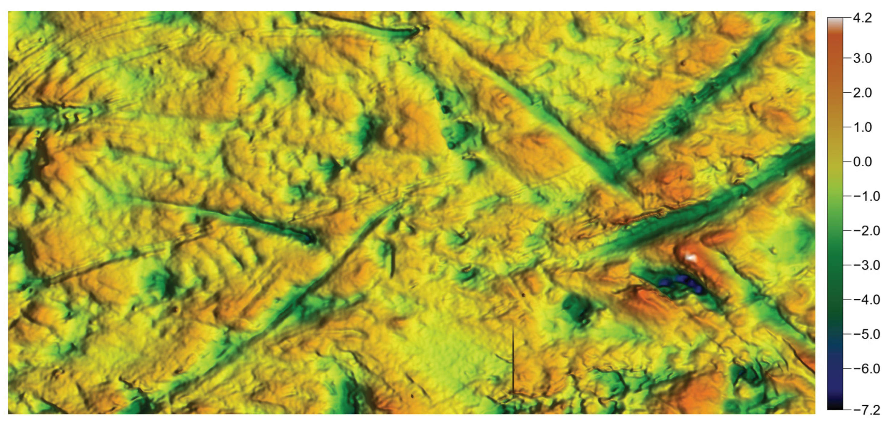
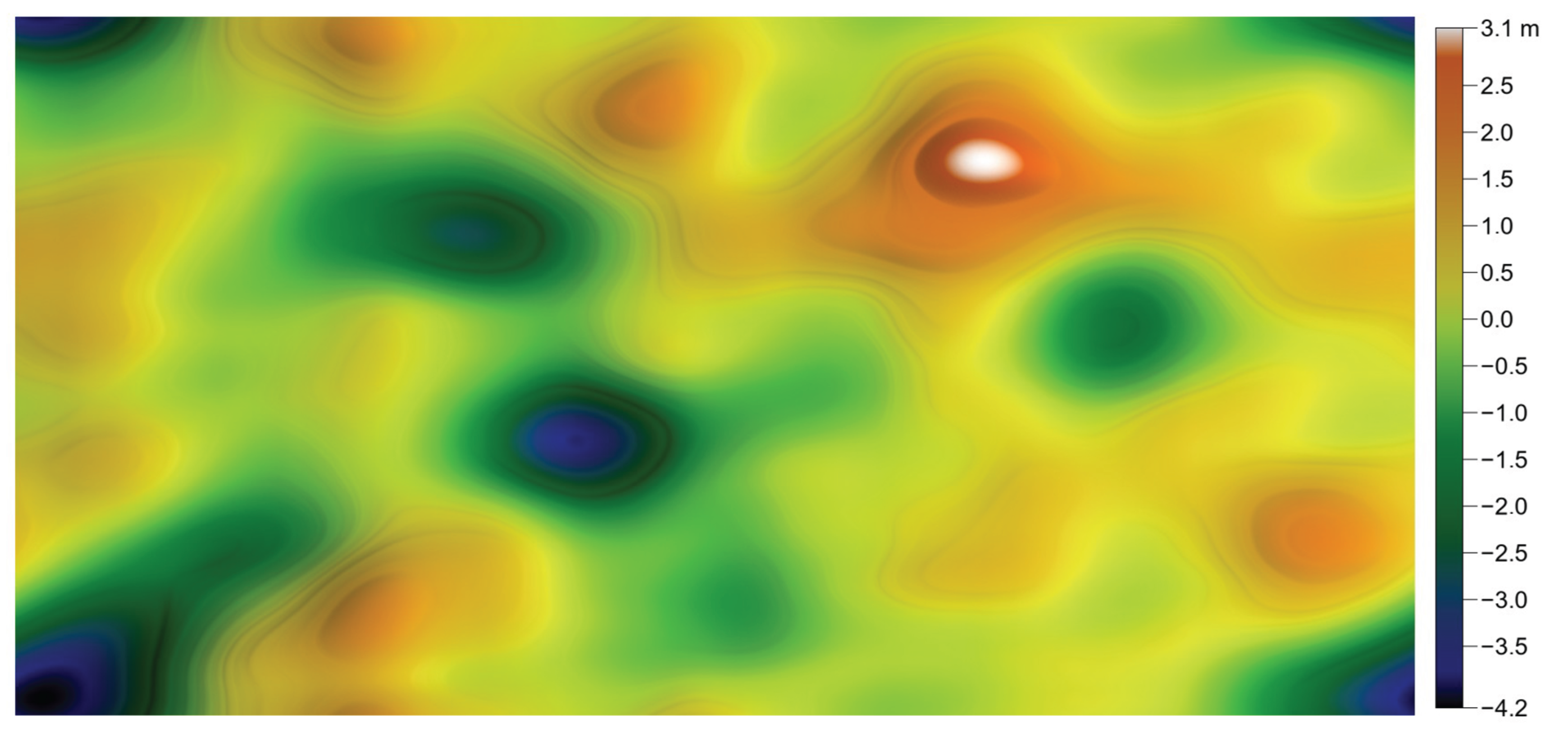
Industrial rough surfaces used to test the algorithm. The white ellipses are the autocorrelation functions cut at . Note that stands for .
Figure 10.
Industrial rough surfaces used to test the algorithm. The white ellipses are the autocorrelation functions cut at . Note that stands for .
Figure 11.
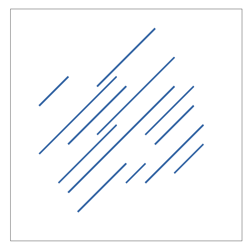
Localized scratches that cannot result from a convolution operator applied to homogeneous noise.
Figure 11.
Localized scratches that cannot result from a convolution operator applied to homogeneous noise.
Figure 12.
Generated rough surface showing the impact of the non-periodicity.
Figure 12.
Generated rough surface showing the impact of the non-periodicity.
Figure 13.
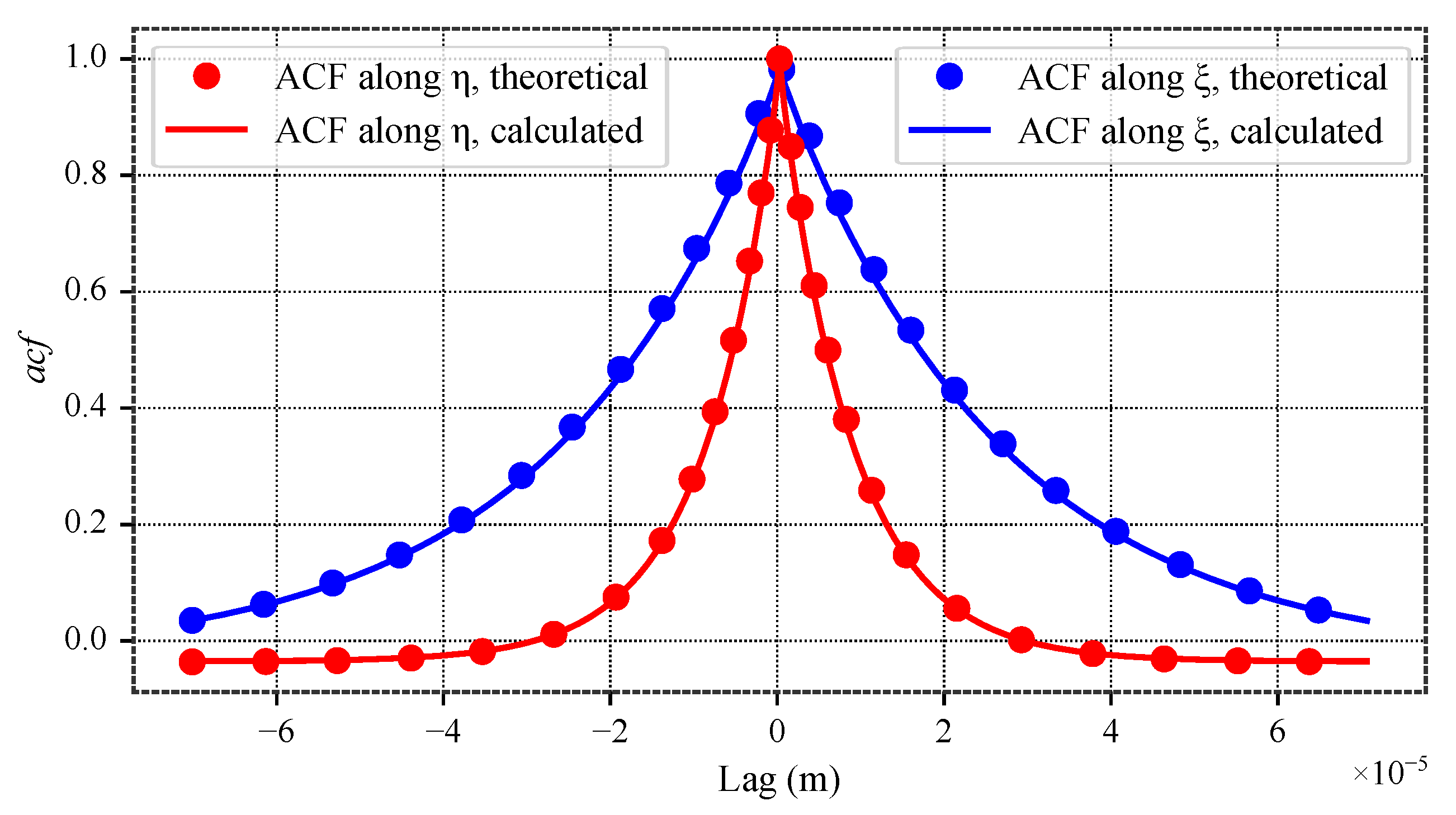
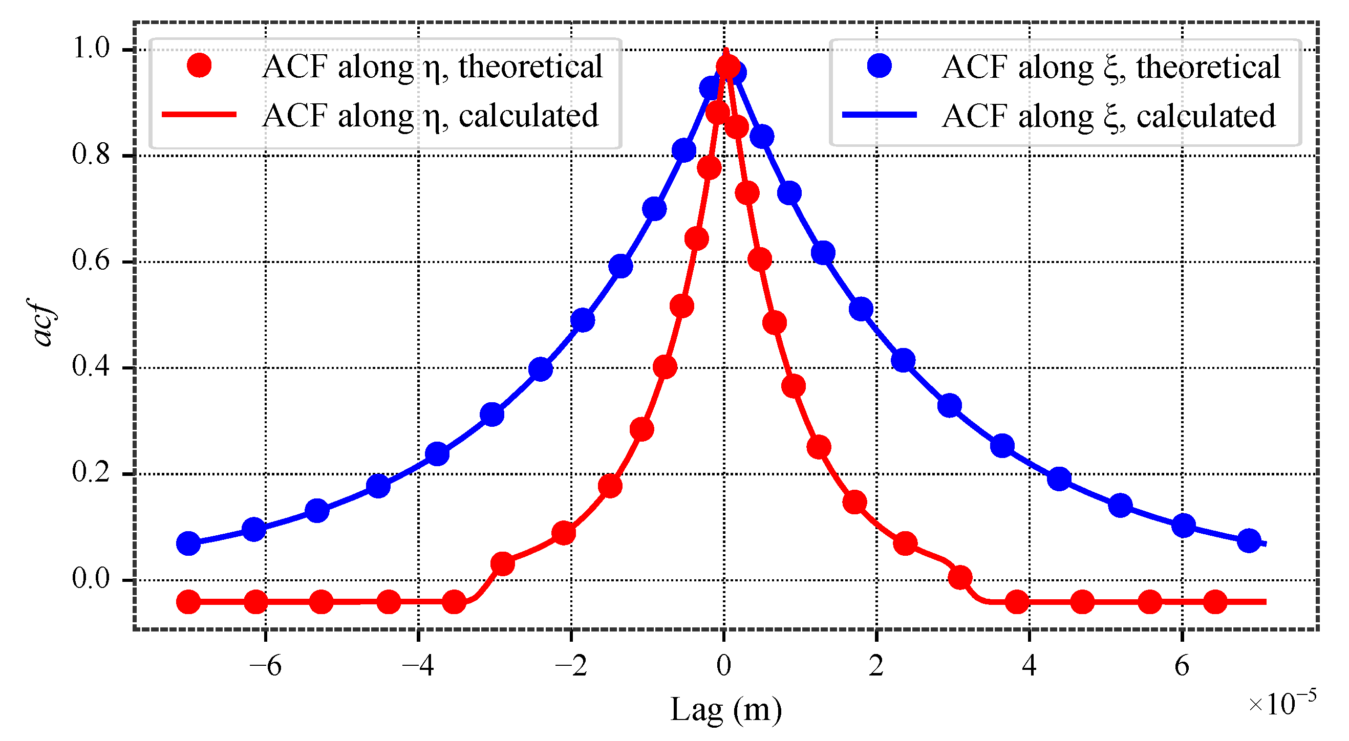
Autocorrelation functions along principal axes and .
Figure 13.
Autocorrelation functions along principal axes and .
Figure 14.
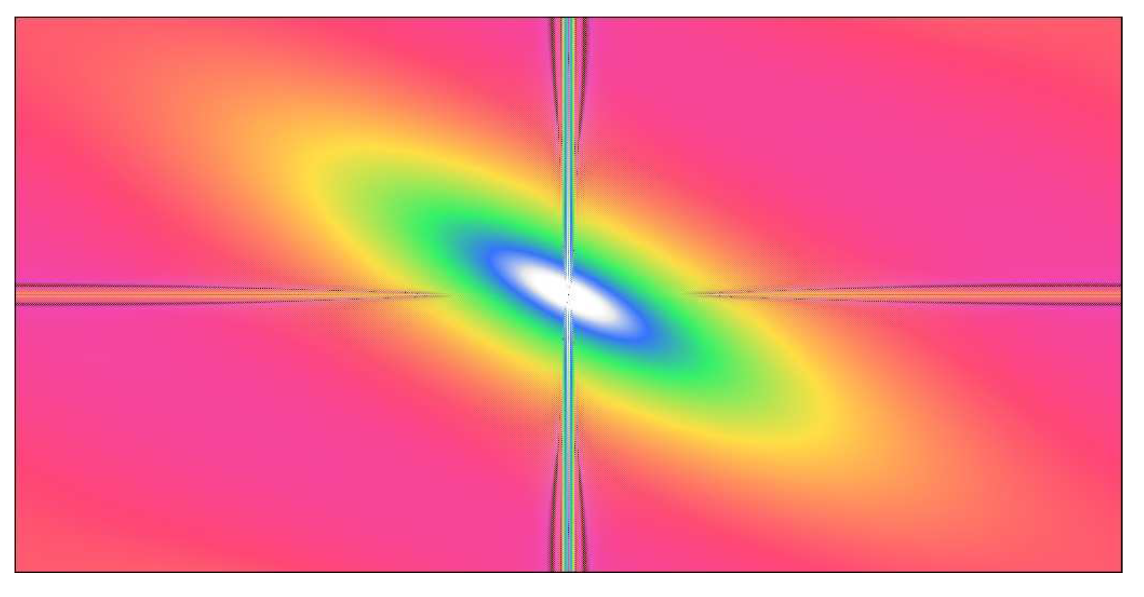
Power spectral density of the dental surface that emphasies the non-periodicity. Scales are irrevelant here, as the information is qualitative.
Figure 14.
Power spectral density of the dental surface that emphasies the non-periodicity. Scales are irrevelant here, as the information is qualitative.
Figure 15.
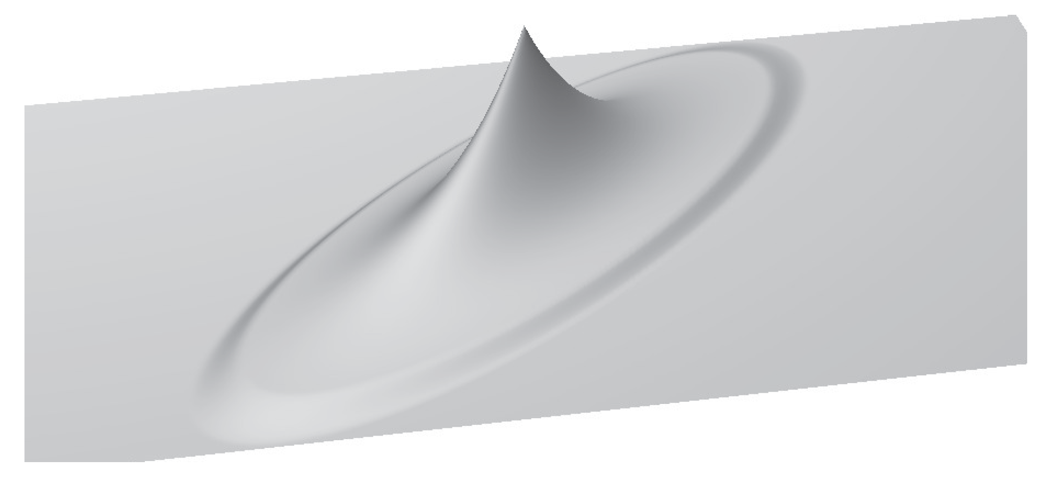
Autocorrelation function in 3D view, showing the effect of the modified Tukey window.
Figure 15.
Autocorrelation function in 3D view, showing the effect of the modified Tukey window.
Figure 16.
Generated surface after apodization and a smooth iterative process initiation.
Figure 16.
Generated surface after apodization and a smooth iterative process initiation.
Figure 17.
Generated non-periodic surface.
Figure 17.
Generated non-periodic surface.
Figure 18.
Autocorrelation functions of the non-periodic surface.
Figure 18.
Autocorrelation functions of the non-periodic surface.
Figure 19.
Autocorrelation functions along and for the dental surface.
Figure 19.
Autocorrelation functions along and for the dental surface.
Figure 20.
Basic reproduction of the dental surface showing spectral leakage.
Figure 20.
Basic reproduction of the dental surface showing spectral leakage.
Figure 21.
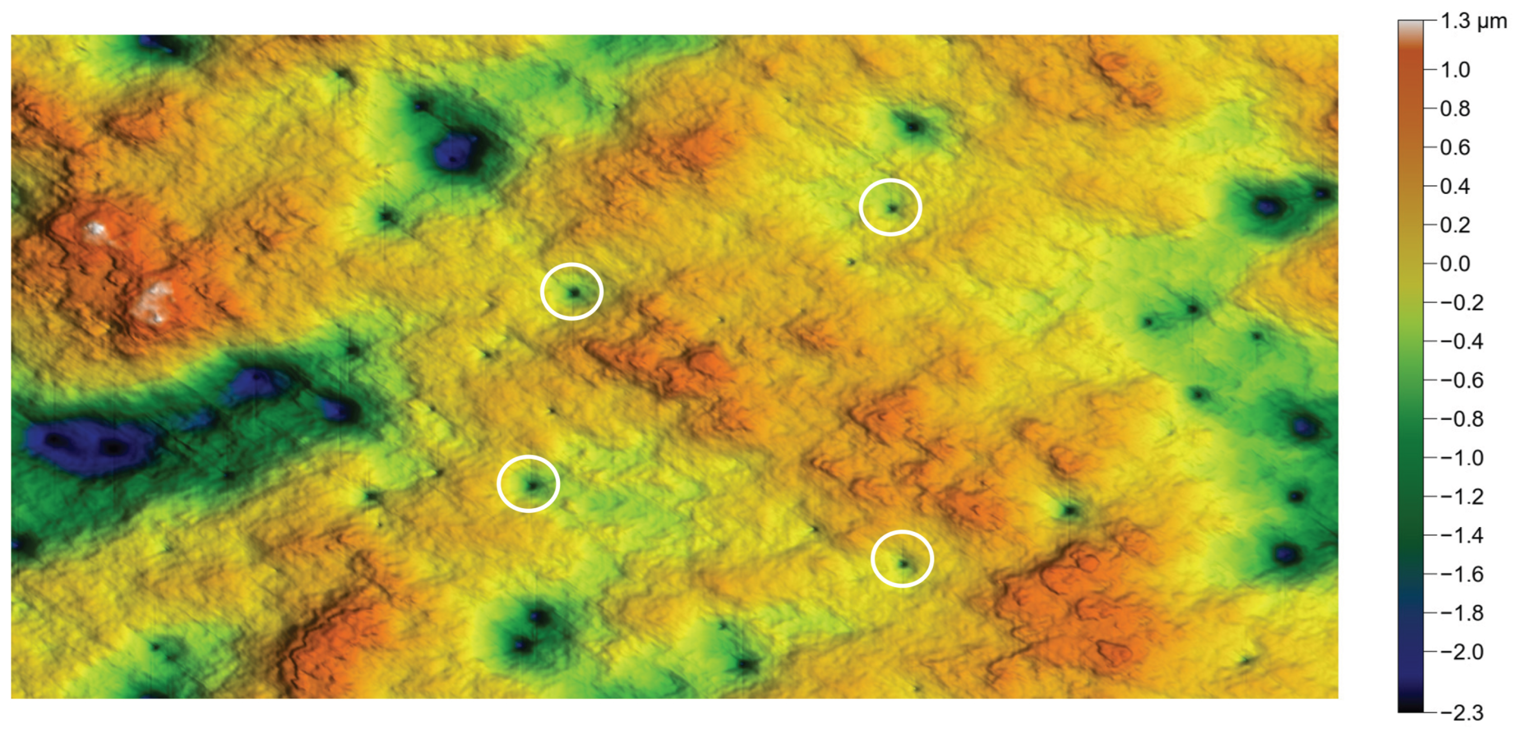
Reproduction of the dental surface after apodization, showing spurious pits (white circles).
Figure 21.
Reproduction of the dental surface after apodization, showing spurious pits (white circles).
Figure 22.
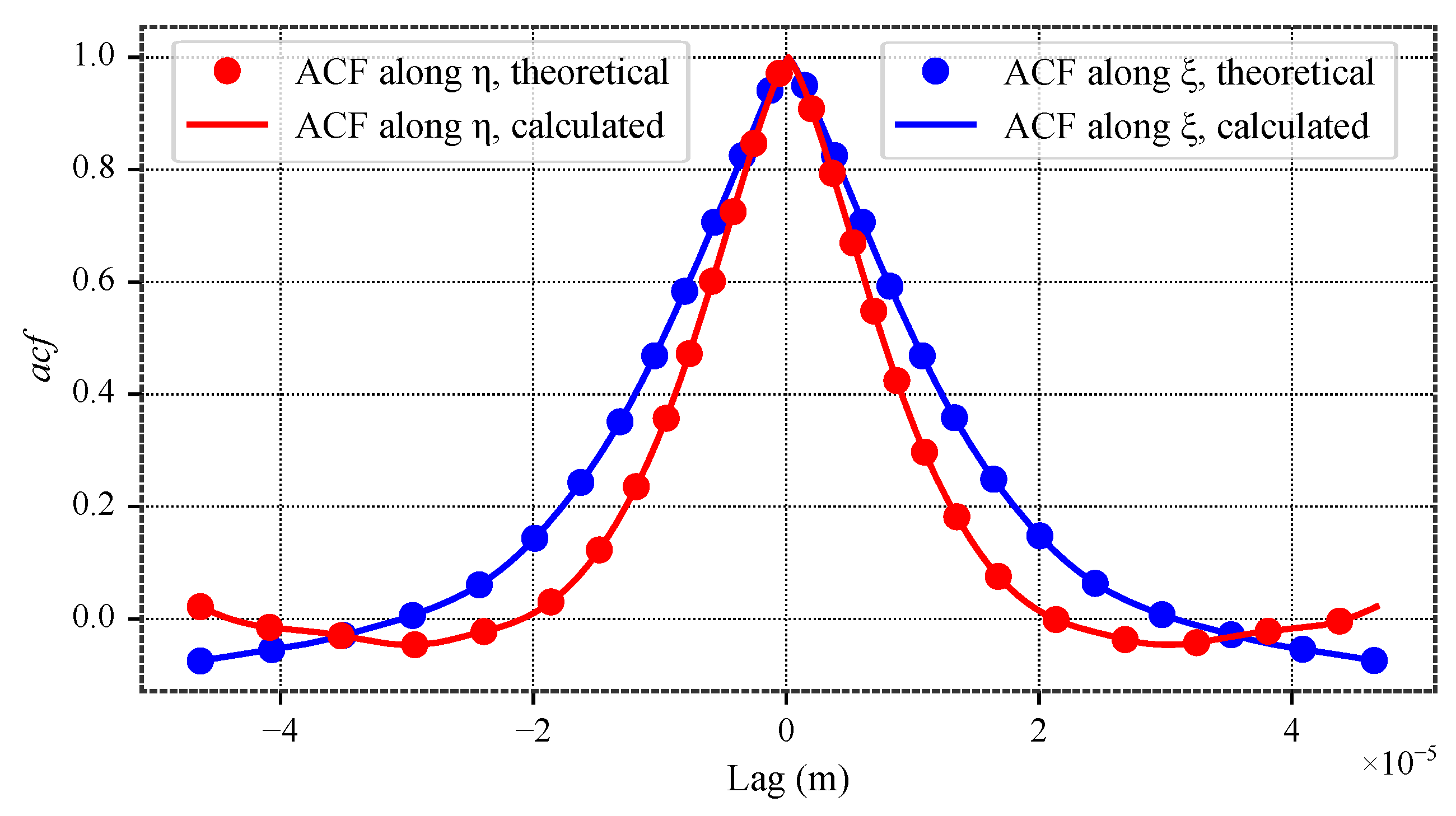
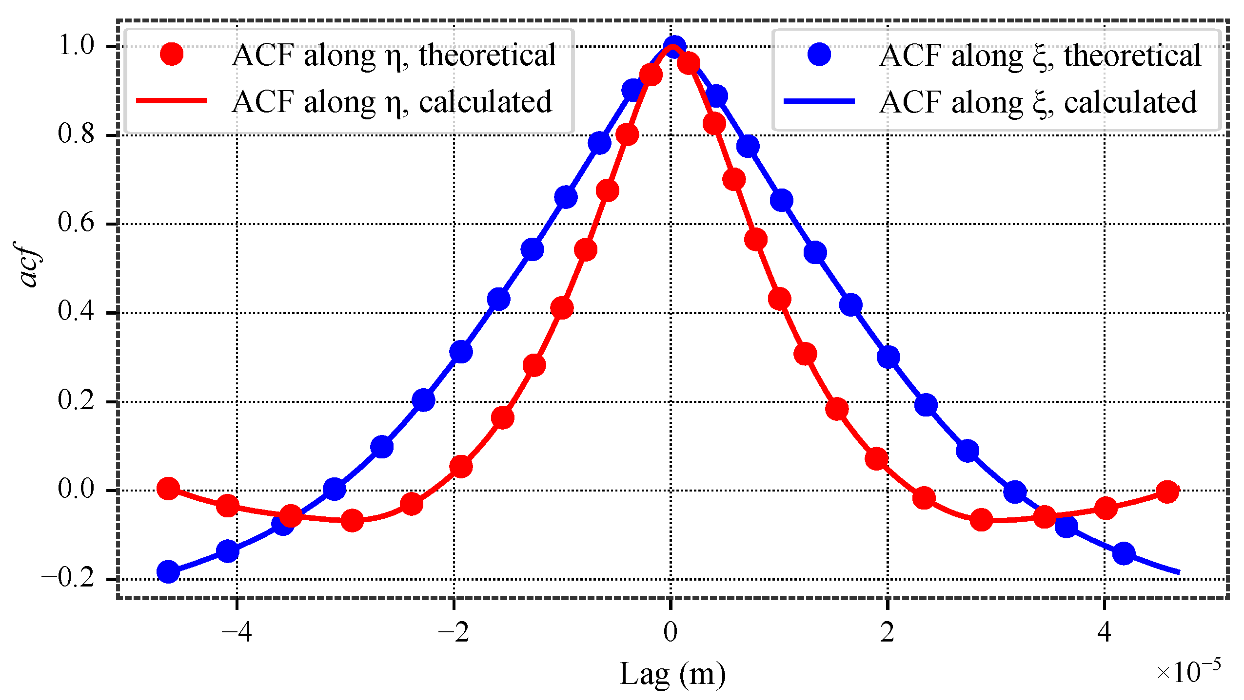
Autocorrelation functions along and after apodization, showing its limited impact.
Figure 22.
Autocorrelation functions along and after apodization, showing its limited impact.
Figure 23.
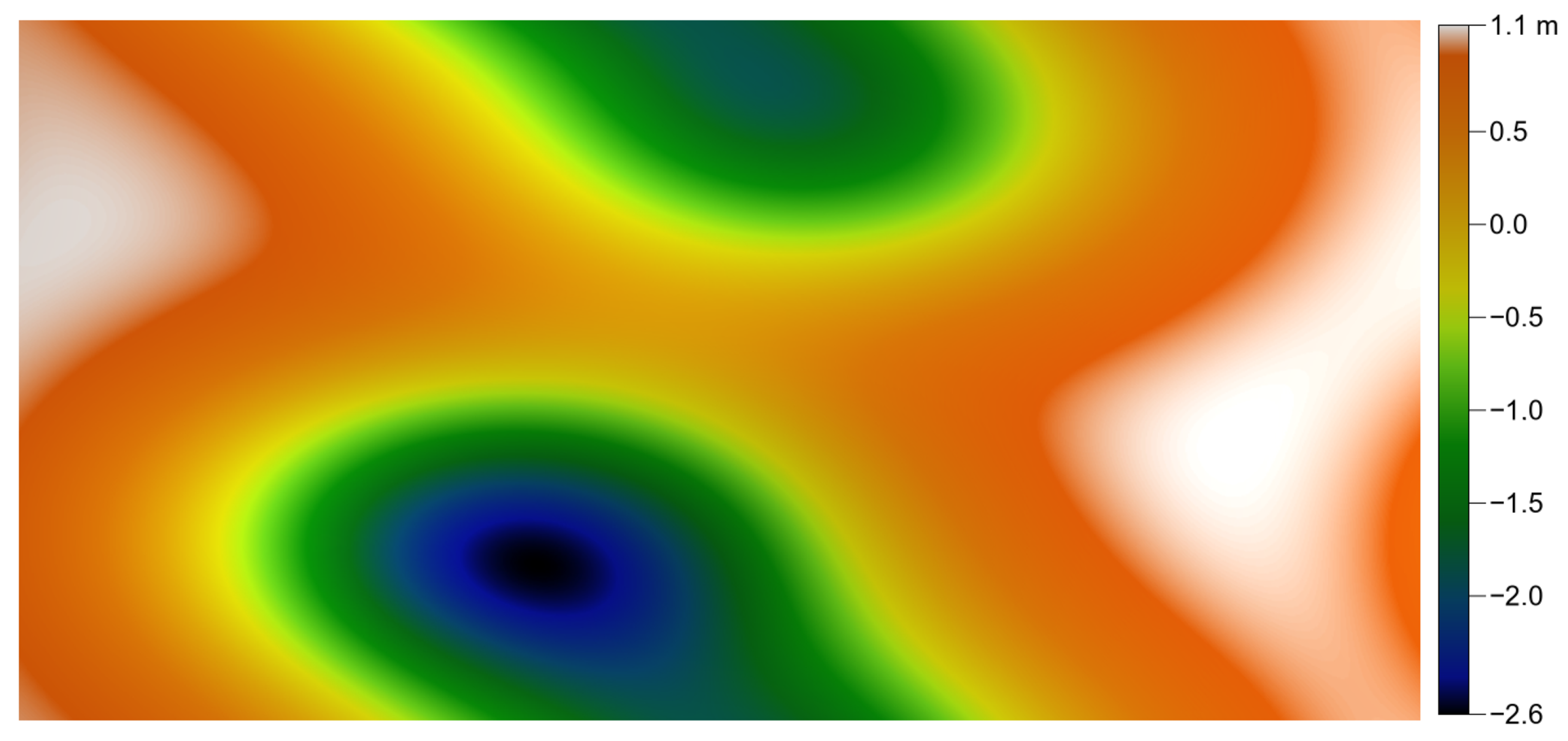
Smooth topography for the iterative process initiation.
Figure 23.
Smooth topography for the iterative process initiation.
Figure 24.
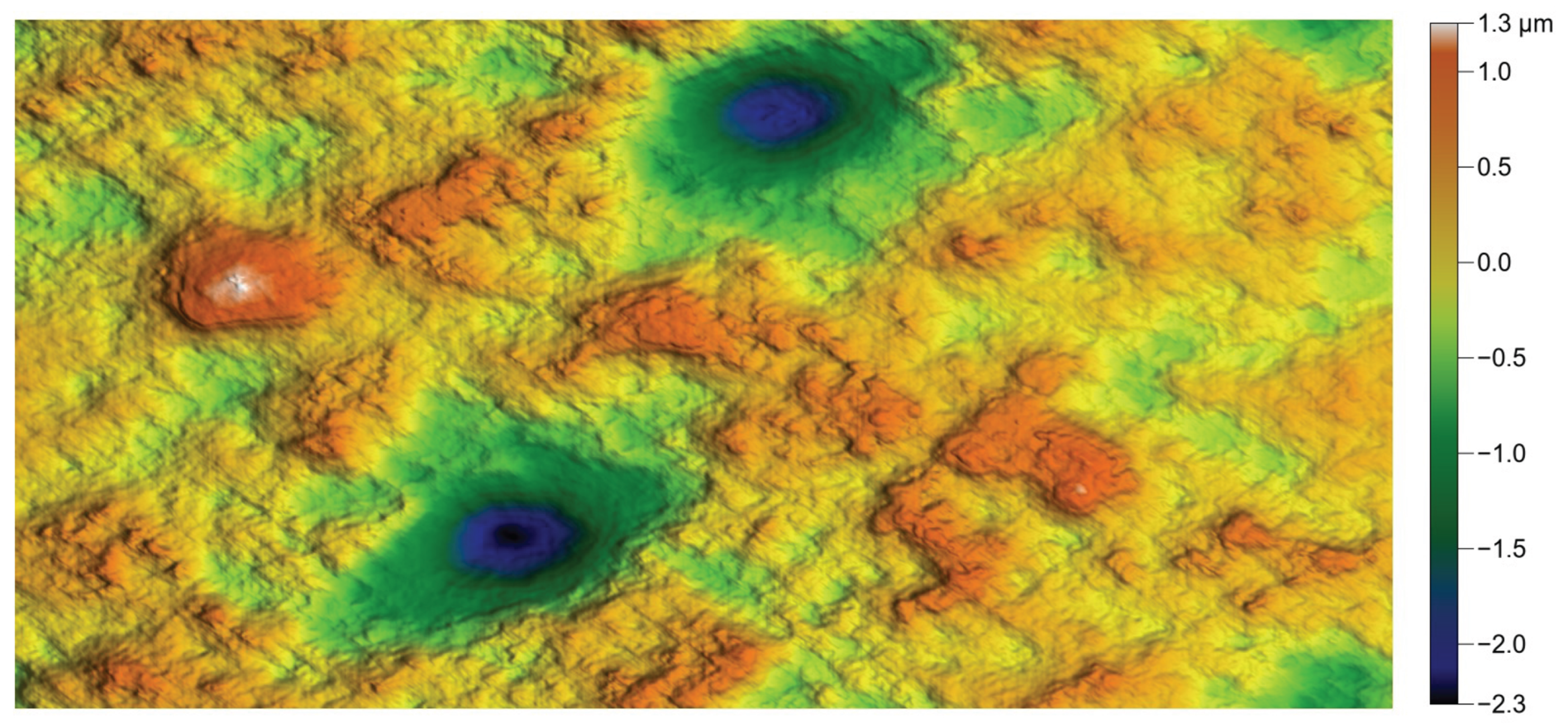
Reproduction of the dental surface with the smoothing texture.
Figure 24.
Reproduction of the dental surface with the smoothing texture.
Figure 25.
Reproduction of the milled surface.
Figure 25.
Reproduction of the milled surface.
Figure 26.
Reproduction of the ground surface.
Figure 26.
Reproduction of the ground surface.
Figure 27.
Reproduction of the polished surface, showing a lack of high and flat areas, resulting from the polishing process.
Figure 27.
Reproduction of the polished surface, showing a lack of high and flat areas, resulting from the polishing process.
Figure 28.
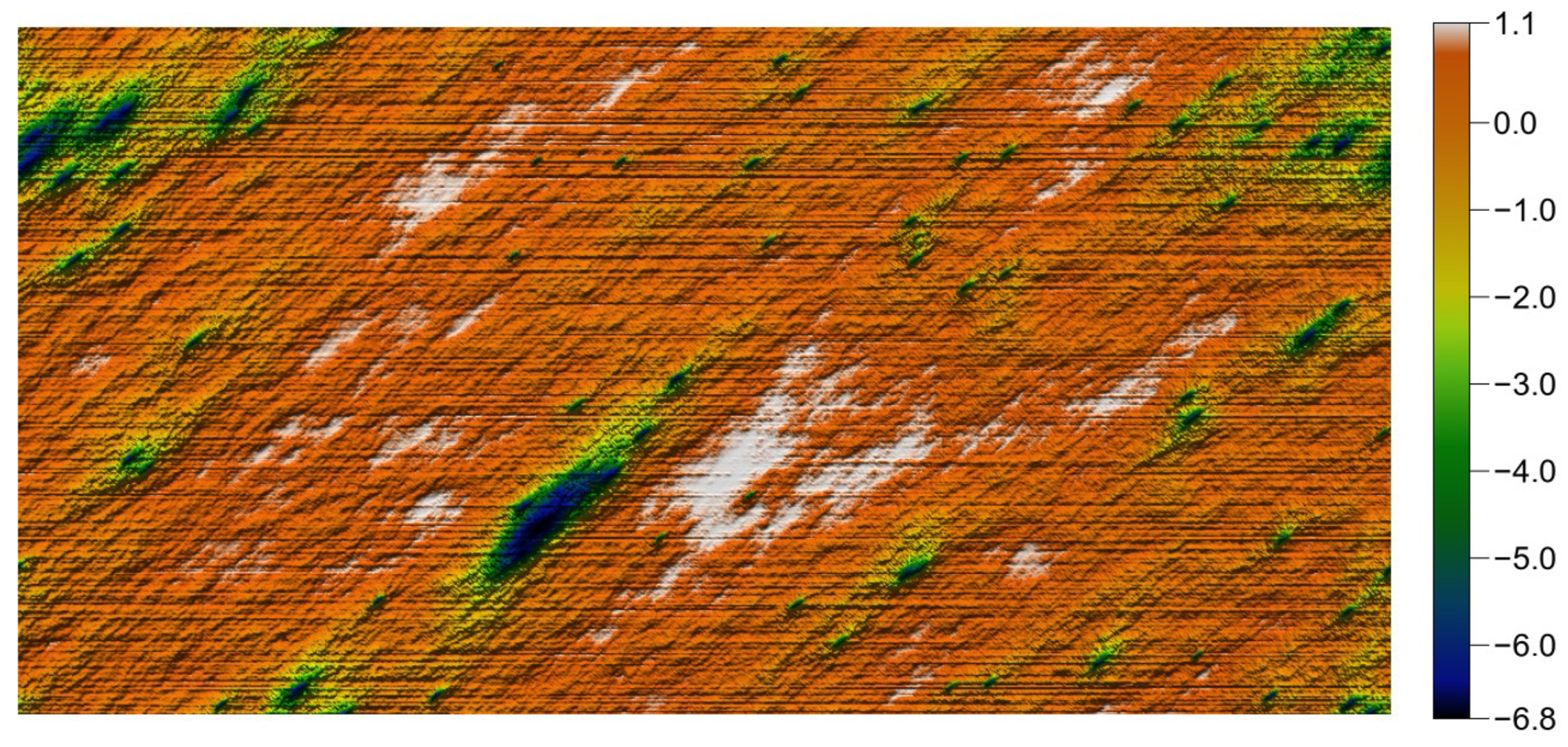
Reproduction of the rotor worn surface. Here again, flat areas should be observed.
Figure 28.
Reproduction of the rotor worn surface. Here again, flat areas should be observed.
Figure 29.
Reproduction of the dental surface after top-hat low-pass filter.
Figure 29.
Reproduction of the dental surface after top-hat low-pass filter.
Figure 30.
Dental surface: low frequencies (LF).
Figure 30.
Dental surface: low frequencies (LF).
Figure 31.
Dental surface: high frequencies (HF).
Figure 31.
Dental surface: high frequencies (HF).
Figure 32.
Reproduction of the LF dental surface.
Figure 32.
Reproduction of the LF dental surface.
Figure 33.
Reproduction of the HF dental surface.
Figure 33.
Reproduction of the HF dental surface.
Figure 34.
Final result after combination of BF and HF results.
Figure 34.
Final result after combination of BF and HF results.
Figure 35.
Reproduction of the dental surface with added scratches.
Figure 35.
Reproduction of the dental surface with added scratches.
Figure 36.
Reproduction of a polished mirror-like industrial surface.
Figure 36.
Reproduction of a polished mirror-like industrial surface.
Table 1.
An example illustrating the limitations of the relations in Equation (
4).
Table 1.
An example illustrating the limitations of the relations in Equation (
4).
| Width (m) | Height (m) | w | h | | | (m) | (m) |
|---|
| 200.0 | 200.0 | 1024 | 1024 | −3.0 | 15.0 | 30.0 | 30.0 |
Table 2.
Resulting statistics
and
with the parameters shown in
Table 1.
Table 2.
Resulting statistics
and
with the parameters shown in
Table 1.
| | | |
|---|
| 21.8 | 1537.3 | −141.0 | 8187.9 |
Table 3.
Qualitative overview of the six surfaces, highlighting the difficulty of each characteristic.
Table 3.
Qualitative overview of the six surfaces, highlighting the difficulty of each characteristic.
| Surface | Non-Gaussian | Anisotropy | Correlation Length |
|---|
| Dental | | − | |
| Rotor | | | − |
| Milled | | | |
| Ground | − | | − |
| Polished | + | + | |
| Mirror-polished | | − | − |
Table 4.
Changes in spatial parameters with and without surface windowing. : fastest decay rate. : Texture aspect ratio. : Texture direction.
Table 4.
Changes in spatial parameters with and without surface windowing. : fastest decay rate. : Texture aspect ratio. : Texture direction.
| Surface | Windowing | (m) | | (°) |
|---|
| Original | – | 5.22 | 7.00 × 10⁻¹ | −13.0 |
| Reproduced, Figure 20 | no | 5.23 | 7.00 × 10⁻¹ | −13.0 |
| Reproduced, Figure 21 | yes | 5.87 | 5.58 × 10⁻¹ | −19.0 |
Table 5.
Comparison of hybrid and spatial parameters between the original and the reproduced surface—dental surface case.
Table 5.
Comparison of hybrid and spatial parameters between the original and the reproduced surface—dental surface case.
| Surface | (%) | | | (m) | | () |
|---|
| Original | 4.30 × 101 | 1.70 × 10⁻² | 2.29 | 5.87 | 5.57 × 10⁻¹ | 19.0 |
| Reproduced | 2.39 × 101 | 2.08 × 10⁻² | 2.61 | 5.87 | 5.58 × 10⁻¹ | 19.0 |
Table 6.
Comparison of hybrid and spatial parameters between the original and the reproduced surface—milled surface case.
Table 6.
Comparison of hybrid and spatial parameters between the original and the reproduced surface—milled surface case.
| Surface | (%) | | | (m) | | () |
|---|
| Original | 2.16 × 101 | 1.12 × 10⁻¹ | 4.45 × 101 | 2.40 × 101 | 1.01 × 10⁻¹ | 6.0 |
| Reproduced | 1.25 × 101 | 1.46 × 10⁻¹ | 5.80 × 101 | 2.35 × 101 | 9.50 × 10⁻² | 6.0 |
Table 7.
Comparison of hybrid and spatial parameters between the original and the reproduced surface—ground surface case.
Table 7.
Comparison of hybrid and spatial parameters between the original and the reproduced surface—ground surface case.
| Surface | (%) | | | (m) | | () |
|---|
| Original | 3.43 × 101 | 9.63 × 10⁻² | 1.75 × 101 | 5.40 | 4.99 × 10⁻² | 47.0 |
| Reproduced | 1.12 × 101 | 1.06 × 10⁻¹ | 2.00 × 101 | 5.38 | 4.95 × 10⁻² | 47.0 |
Table 8.
Comparison of hybrid and spatial parameters between the original and the reproduced surface—polished surface case.
Table 8.
Comparison of hybrid and spatial parameters between the original and the reproduced surface—polished surface case.
| Surface | (%) | | | (m) | | () |
|---|
| Original | 1.00 × 10² | 2.12 × 10⁻⁶ | 2.81 × 10⁻⁴ | 2.66 × 101 | 4.89 × 10⁻¹ | −10.0 |
| Reproduced | 1.00 × 10² | 2.15 × 10⁻⁶ | 2.94 × 10⁻⁴ | 2.63 × 101 | 4.90 × 10⁻¹ | −10.0 |
Table 9.
Comparison of hybrid and spatial parameters between the original and the reproduced surface—rotor surface case.
Table 9.
Comparison of hybrid and spatial parameters between the original and the reproduced surface—rotor surface case.
| Surface | (%) | | | (m) | | () |
|---|
| Original | 9.59 × 101 | 2.64 × 10⁻³ | 4.37 × 10⁻¹ | 4.10 | 7.75 × 10⁻¹ | 3.0 |
| Reproduced | 9.31 × 101 | 2.92 × 10⁻³ | 4.80 × 10⁻¹ | 4.05 | 7.74 × 10⁻¹ | 3.0 |
Table 10.
Changes in spatial and height parameters after top-hat smoothing.
Table 10.
Changes in spatial and height parameters after top-hat smoothing.
| Windowing | (m) | (m) | (m) | (m) | (m) | | | (m) | | () |
|---|
| no | −2.31 | 1.25 | 6.84 × 10⁻² | 3.46 × 10⁻¹ | 4.85 × 10⁻¹ | −1.20 | 6.02 | 5.86 | 5.58 × 10⁻¹ | 19 |
| yes | −2.14 | 1.14 | 7.23 × 10⁻² | 3.45 × 10⁻¹ | 4.85 × 10⁻¹ | −1.27 | 6.07 | 6.12 | 5.64 × 10⁻¹ | 19 |
Table 11.
Comparison of hybrid and spatial parameters between the original and the reproduced surface—polished mirror-like surface case.
Table 11.
Comparison of hybrid and spatial parameters between the original and the reproduced surface—polished mirror-like surface case.
| Surface | (%) | | | (m) | | () |
|---|
| Original | 1.00 × 10² | 3.10 × 10⁻⁶ | 6.48 × 10⁻⁴ | 9.38 | 6.67 × 10⁻¹ | −34.0 |
| Reproduced | 1.00 × 10² | 2.92 × 10⁻⁶ | 6.12 × 10⁻⁴ | 9.07 | 6.67 × 10⁻¹ | −34.0 |
