


Abstract
The two most severe cosmological tensions in the Hubble constant and the matter clustering amplitude have the same relative discrepancy of 8.3%, which suggests that they may have a common origin. Modifications of gravity and exotic dark fields with numerous free parameters introduced in the Einstein field equations often struggle to simultaneously alleviate both tensions; thus, we need to look for a common cause within the standard CDM framework. At the same time, linear perturbation analyses of matter in the expanding CDM universe have always neglected the impact of comoving peculiar velocities (generally thought to be a second-order effect), the same velocities that, in physical space, cannot be fully accounted for in the observed late-time universe when the cosmic distance ladder is used to determine the local value of . We have reworked the linear density perturbation equations in the conformal Newtonian gauge (sub-horizon limit) by introducing an additional drag force per unit mass in the Euler equation with , where is a positive dimensionless constant and is the time-dependent Hubble friction. We find that a damping parameter of is sufficient to resolve the tension by suppressing the growth of structure at low redshifts, starting at to achieve , respectively. Furthermore, we argue that the physical source causing this additional friction (a tidal field generated by nonlinear structures in the late-time universe) is also responsible for a systematic error in the local determinations of —the inability to subtract peculiar tidal velocities along the lines of sight when determining the Hubble flow via the cosmic distance ladder. Finally, the dual action of the tidal field on the expanding background—reducing both the matter and the dark energy sources of the squared Hubble rate , thereby holding back the cosmic acceleration —is of fundamental importance in resolving cosmological tensions and can also substantially alleviate the density coincidence problem.
1. Introduction
1.1. Standard CDM Model
The standard CDM cosmological model has enjoyed remarkable success over the past two decades, providing a consistent framework that explains a vast array of observations, from the temperature anisotropies of the cosmic microwave background (CMB) to the large-scale distribution of galaxies [1,2]. Based on a spatially flat universe dominated by cold dark matter (CDM) and a cosmological constant [3,4,5,6], the CDM model is specified by six parameters, which have been constrained with sub-percent precision by the Planck satellite mission [1]. On the other hand, the cosmological constant itself presents one of the most profound theoretical challenges in physics today, known by its components as the cosmological constant problem (CCP) and the density coincidence problem (DCP), respectively [7,8].
- (1)
- CCP: Quantum field theory predicts a vacuum energy density vastly greater than the observed value by more than 120 orders of magnitude [9,10].
- (2)
- DCP: The effective density corresponding to and the density of matter are comparable at the present epoch, requiring highly contrived initial conditions to reach this universal state [11,12].
These fundamental puzzles motivate a search for cosmological mechanisms that can drive the late-time acceleration of the universe without relying on extreme fine-tuning assumptions.
1.2. Major Cosmological Tensions
As observational precision has improved over the years, some statistically significant cracks have appeared in the CDM foundation. In particular, two major discrepancies have persisted and intensified, suggesting the presence of systematic errors in diverse observational datasets and the need for more physics unaccounted for in CDM—or, alternatively, the necessity to modify gravity at large scales by including exotic new physics and more dark, undetected fields in cosmological theories [13,14,15].
The first and most prominent discrepancy is the “Hubble tension”, concerning the value of the current expansion rate . Estimates of inferred from early-universe physics (CMB) assuming CDM consistently yield lower values of km s−1 Mpc−1 [1]. In stark contrast, local late-universe measurements using the cosmic distance ladder (CDL) consistently favor a higher value of km s−1 Mpc−1 [15,16,17]. The statistical significance of this discrepancy has reached the level, rendering it impossible to dismiss as a mere statistical fluctuation [16].
The second major discrepancy is the “ tension”, which involves the clumpiness of baryonic matter observed in the late universe. The parameter quantifies the amplitude of density fluctuations. Predictions based on Planck CMB data project a relatively high degree of clustering () [1]. Conversely, direct measurements of late-time large-scale structure (LSS) from weak gravitational lensing and galaxy clustering surveys, such as the Kilo-Degree Survey (KiDS) [18] and the Dark Energy Survey (DES) [19], consistently measure a lower amplitude (–0.78). The growth history of the LSS provides a powerful test of the background evolution [20]. While the statistical significance of this tension (∼2–3) is lower than that of , its persistence across independent low-redshift probes suggests a genuine physical anomaly: our universe is smoother than what CDM predicts.
1.3. A Remarkable Coincidence and a New Path Forward
In this work, we first highlight a striking coincidence that has largely gone unnoticed: the relative difference in the two major tensions is virtually identical.
- (a)
- The relative discrepancy in [1,15,16] is
- (b)
- The relative discrepancy in [1,15,18] is
We argue that this concordance in relative discrepancies is not coincidental. Rather, it points toward a single underlying physical mechanism responsible for both cosmological tensions. The missing physics ought to be capable of simultaneously (i) suppressing the predicted LSS growth rates by about 8.3% and (ii) resolving the 8.3% overestimate of that currently appears in the local CDL measurements.
While numerous extensions to CDM have been proposed—ranging from early dark energy [21] to modified gravity theories [22] and models involving coupled dark sectors [23]—these solutions typically introduce complex exotic fields with multiple free parameters, a generally undesirable trade-off. Furthermore, such fields often struggle to resolve both tensions simultaneously; mechanisms that alleviate the tension frequently exacerbate the tension [24,25]. For these reasons, we choose to improve CDM without invoking new exotic physics.
To this end, we revisit the standard model, searching for minimal adjustments that could simultaneously account for both of the above ∼8.3% tensions, and we consider linear density perturbations within this framework [10,26]. Standard treatments typically assume a perfect cosmic fluid of collisionless dust, in which perturbations grow by gravitational instability [27], while gravitational attraction is counteracted to a degree by the Hubble flow. The fluid peculiar velocities affecting the linear density perturbations have traditionally been neglected in the linearized Euler equation (as a nonlinear effect [28,29]), even in the low-redshift universe when the cosmic deceleration has significantly diminished. But peculiar velocities are also sources of noise and uncertainty that complicate the determination of recession velocities in the local CDL measurements [30]. Thus, if tidal interactions from exterior nonlinear structures introduce radial velocities into the linear regime at late times [28], the resulting drag forces could systematically distort our interpretations of both key local rates—the background expansion rate and the LSS growth rate .
Based on the above reasoning, we test a modification of the linear perturbation equation in the sub-horizon limit of the conformal Newtonian gauge by introducing a first-order drag force proportional to the amplitude of the peculiar velocity itself. This drag acts as an additional friction that somewhat suppresses the growth of structure. In this paper, we demonstrate that a drag amplitude of at low redshifts, along with the Hubble friction , is sufficient to suppress the LSS growth rate and resolve the tension. Furthermore, we argue that the same mechanism may account for the apparent excess in the locally measured values, thereby offering a unified “CDM” resolution of the two major tensions in modern CDM cosmology and other identified discrepancies [15].
1.4. Outline
The remainder of this paper is organized as follows:
- In Section 2, we introduce an additional drag term to the Euler equation and perform the linear perturbation analysis in the conformal Newtonian gauge within the FLRW background.
- In Section 3, we determine typical values of in our modified CDM framework and we examine whether the tension can be resolved by accounting for the added time-dependent friction (% of ) induced by drag forces due to an exterior tidal field (statistically isotropized, but with a nonzero mean value).
- In Section 4, we examine how this kinematic enhancement of the Hubble expansion modifies the background dynamics of the standard CDM model to linear order in .
- In Section 5, we develop a simplified 1D radial line-of-sight model and estimate the net tidal acceleration acting on a target galaxy, as well as the implied magnitude of .
- In Section 6, we summarize our conclusions.
- In Appendix A, we show that the modifications introduced to the kinematics and the dynamics of the Hubble flow are consistent with one another.
2. Linear Perturbations with a Time-Dependent Drag Force
We formulate the linear scalar perturbation equations for an FLRW universe with dust, a cosmological constant, and a time-dependent drag force due to a peculiar velocity field. The analysis is performed in comoving spatial coordinates and cosmic time t. The background dynamics follows the standard spatially flat CDM model, while the perturbations obey modified Euler dynamics due to the additional friction term.
2.1. Initial Assumptions and Kinematic Framework
We consider a spatially flat FLRW spacetime with line element
where is the scale factor and c is the speed of light in vacuum. The background expansion rate is given by the Hubble function
The matter sector is assumed to be a pressureless perfect fluid (dust) with background density satisfying the continuity equation
The background evolution of , and is governed by the usual Friedmann equations (FEs) with a cosmological constant and a gravitational constant G, viz.,
Combining the FEs and using the identity , we obtain the Raychaudhuri–Landau equation for [31], viz.,
This equation relates the cosmic acceleration with the Hubble expansion rate H and the cosmological constant .
2.2. Linearized Perturbation Equations
2.2.1. Preliminaries
In the FLRW background, we introduce small perturbations to linear order. The density field is decomposed as
where is the density contrast in comoving coordinates .
The gravitational potential , which encodes the perturbation of the metric sourced by these density fluctuations, represents the scalar metric perturbation in the conformal Newtonian gauge. In the Newtonian (sub-horizon) limit, where time derivatives of the metric potentials are negligible and spatial gradients dominate, the linearized fluid equations reduce to their familiar comoving Newtonian forms. In this regime, satisfies the standard Poisson equation relating the gravitational potential to the comoving density perturbations [10,26].
The proper velocity of the fluid relative to an observer at the origin is defined as . We decompose into the Hubble flow and the peculiar velocity as
where is the Hubble rate and . The peculiar velocity measures departures from the pure Hubble flow and is related to the comoving coordinates by
The perturbed Euler equation is modified by the introduction of a time-dependent drag force per unit mass . When expressed in terms of the peculiar velocity, this physical deceleration is assumed to take the form
where is an arbitrary non-negative function of cosmic time with the dimension of frequency. This ensures that the friction enters the linear growth equation as an additive damping term.
2.2.2. First-Order Equations
To first order in the quantities , and Φ, the continuity, Euler, and Poisson equations for a fluid of dust subject to the time-dependent drag deceleration (Equation (10)), respectively, are
This system of equations is closed and can be reduced to a single differential equation for the linear growth of density perturbations : We define the comoving divergence of peculiar velocities
which represents the rate at which the fluid is fluctuating in comoving space. The continuity Equation (11) then becomes
Next, taking the comoving divergence of the Euler Equation (12), we obtain the equation
and, substituting from the Poisson Equation (13) and from Equation (15), we obtain the final form
Equation (17) is an ordinary differential equation (ODE) that governs the cosmic evolution of a linear density Fourier mode with comoving wavenumber k. Because the perfect fluid is assumed to be dust, the evolution of becomes independent of k on sub-horizon scales [32]. In this sense, this equation generalizes the standard CDM growth equation by including the friction coefficient . This term enhances the conventional Hubble friction and results in greater suppression of the growth of linear density perturbations relative to the growth in the standard CDM model with .
2.3. Scaling the Friction Coefficient
In the subsequent analysis, we scale to the expansion-induced Hubble friction with coefficient . We adopt the convenient form
where is a dimensionless constant parameterizing the strength of the drag forces relative to the usual Hubble damping term. This choice ensures that the added friction is naturally scaled to the universal expansion, thereby simplifying further investigations. It is, however, expected that .
Substituting Equation (18) into Equation (17), we find that the evolution of the density contrast satisfies the linear differential equation
Naturally, for , we recover the standard CDM linear growth Equation [10,26].
The scaling constant in Equation (19) naturally provides a framework for addressing the observed tension, and it may also potentially alleviate the tension. In the following section, we determine the range of values that reconcile the predicted linear growth with current observational constraints on 0.76–0.78) [15].
3. Clustering Amplitudes and Growth Rates in CDM with a Drag Force
3.1. Preliminaries
The linear growth factor (D) of structure is commonly defined in terms of the matter density contrast [10,26], viz.,
where is usually taken to be the scale factor at recombination (redshift ). For this reason, we introduce the scale factor as the independent variable in the ODE (19) for the matter density contrast, as shown in Section 3.2 and Section 3.3 below. For the calculations, we also adopt
corresponding to .
The RMS fluctuation amplitude , linearly extrapolated to the present epoch and corresponding to the Planck-2018 CDM normalization [1], is defined in terms of [10,26]. In our modified CDM model, we correspondingly write , which we determine from the scaling relation
where [1].
The observational clustering parameter [1,33] is then determined by the relation
where is the matter density fraction at present time. Our modified model is essentially CDM with enhanced friction, so we adopt the Planck-2018 value of , for which Equation (23) reduces to
precise to six significant digits.
In general, the matter density fraction varies with the scale factor and is defined as [10,26]
where is the background matter density, at present (), and
is the critical density in FLRW cosmology. We note that refers to the total (CDM plus baryonic) matter component; on the linear scales of interest, the growth of structure is dominated by dark matter with baryons acting as passive tracers of the overall gravitational potential wells.
It is convenient to introduce the dimensionless Hubble function , in terms of which the fraction may be written as
which satisfies . The dimensionless Hubble function is given by the well-known relation
where is the vacuum energy fraction at present [1,10,26]. These quantities naturally appear in the gravitational source term of the linear growth equation derived below.
3.2. The ODE of the Matter Density Contrast
We change the independent variable in Equation (19) from cosmic time t to scale factor a [34] by using the identities
Using primes to denote the derivatives with respect to a and replacing from Equation (20), we find that the linear growth equation is transformed into
In this ODE, a factor of effectively enhances the coefficient of Hubble friction (), and the gravitational source term depends on the mean universal density of matter at each instance.
For computational efficiency, it is convenient to also express the coefficient of friction in Equation (30) in terms of . The procedure simplifies the ODE considerably, viz.,
where can be computed from the compact expression
which is derived by combining Equations (27) and (28). Here, the fiducial ratio , precise to seven significant digits [1].
3.3. Analytic Approximation for the Matter-Dominated Epoch
To gain analytic insight into the effect of the enhanced friction parameter , we consider an approximate solution of the growth Equation (31) in the matter-dominated regime. At early times (), Equation (32) implies that , so that Equation (31) reduces to a Cauchy–Euler ODE [35,36], viz.,
which admits power-law solutions of the form , where p is a constant to be determined.
The power of the growing mode, expanded to linear order in , is . Since (Equation (20)), the growing solution of the matter-dominated ODE (33) is
In standard CDM where , and the growing mode is simply .
Extrapolating this solution to the present epoch (), we apply the results to Equation (22) for ; using Equation (21), we find, to linear order, that
and that
The steep slope of in reflects the cumulative effect of a slightly enhanced Hubble friction (by ) over the long timescale from recombination () to today. In a realistic CDM background, this cumulative suppression of growth is expected to be mitigated because the drag forces are expected to become significant only at late times, when the causal nonlinear structures have been formed in the universe and has significantly decreased with time.
Finally, a qualitative comparison with observations may be carried out using Equation (23) for , with the important caveat that the analytic approximations above assume and . Within this framework, small values of the enhanced friction parameter of – reduce the CDM-predicted clustering amplitude and alleviate the tension because the drag forces have been active at all times since recombination. In Section 3.4, we refine this rough estimate by numerically integrating the full growth Equation (31) for a range of values and a range of initial conditions in a realistic CDM background. In these computations, the critical redshift at which drag forces first appear becomes a free parameter.
3.4. Numerical Solutions of the Growth Equation
To obtain precise estimates of the impact of the enhanced Hubble friction parameter on the growth of linear density perturbations for redshifts , we integrate numerically the growth Equation (31). The integration of the growing solution begins in the early matter-dominated regime (standard CDM with and ) at a scale factor corresponding to recombination, viz. , where
The integration is carried out from to an intermediate value of (a free parameter corresponding to ), where the term, the other free parameter, is activated smoothly and persists up to the present epoch (). The numerical algorithm uses the adaptive-step Runge–Kutta solver ode45, which has been widely employed in computational physics [37,38]. This solver automatically adjusts the step size to maintain accuracy, making it suitable for integrating the rapidly varying growth function over many orders of magnitude in scale factor a.
The resulting growth factors at are then used to compute the corresponding linear clustering amplitude via
where is obtained from Equation (24) for and [1], thereby allowing for a direct comparison with observational results.
The numerical solutions are controlled by the two free parameters and (or ) and are grouped into two sets (A and B) according to the chosen typical values of the parameter .
3.4.1. Parameter of the Hubble Friction
In the first set of solutions listed in Table 1, we choose and we determine the critical values of and that result in reduced growth at the present time relative to the standard CDM solution. The reduced growth results in the listed values of , where one-half of the values determined by observations lie [15] (a total of published measurements of , excluding four outliers, with mean and standard deviation ). The complete solution with and that results in (Model A5 in Table 1) is illustrated in Figure 1.
Table 1.
Numerical solutions of the growth Equation (31) with (i.e., 8.3% of the Hubble friction ) at all redshifts .
Figure 1.
The numerical solution with and (red curve) that results in (Model A5 in Table 1). The standard CDM solution is also shown for comparison (blue curve). Both solutions are normalized to the value of the standard CDM solution.
Model A8 is included in Table 1 to accommodate the latest KiDS–Legacy survey that has produced a rather surprising result: and [39,40]. Naturally, a value of is too large for such a small tension versus from CDM, and this is why only a very recent activation redshift of is required in the CDM model to resolve the remaining small discrepancy.1,2
3.4.2. Parameter of the Hubble Friction
In the second set of solutions listed in Table 2, we choose and we analyze critical values of (perhaps a palatable upper limit [28]) that result in reduced growth at the present time. This smaller value of characterizes the smaller tension between standard CDM [1] and a subset of the SnIa-TRGB measurements that have resulted in km s−1 Mpc−1 [15,17]. Evidently, drag forces of such a lower magnitude (only ∼ of the Hubble friction ) are capable of resolving the tension only if truly lies at the high end (∼0.79) of the observational range, and, even then, has to be , a relatively high threshold. The complete solution with and that results in (Model B3 in Table 2) is illustrated in Figure 2.
Table 2.
Numerical solutions of the growth Equation (31) with (i.e., 3.9% of the Hubble friction ) at all redshifts .
Figure 2.
The numerical solution with and (red curve) that results in (Model B3 in Table 2). The standard CDM solution is also shown for comparison (blue curve). Both solutions are normalized to the value of the standard CDM solution.
3.5. Growth Rate from the Nonlinear First-Order Growth ODE
Further characterization of the linear growth of structure is provided by the dimensionless growth rate
where the initial value problem (IVP) for is described by Equations (31), (32), and (38) [26,28].
Recast in terms of , the IVP is described by a nonlinear first-order ODE of the Riccati type, viz.,
along with the initial condition
where . Table 3 summarizes the present-day growth rates obtained for CDM and the CDM Models A1–A8 of Table 1. In general terms, the growth rates of the models are reduced by ≃8%, in contrast to the ratios that are reduced by 5–10%.
The two diagnostics in Table 3, i.e., copied from Table 1 and the new ratio , quantify different aspects of the same growth history.
- Ratio measures an integrated amplitude effect: once is activated at , the enhanced friction suppresses growth over the entire interval , and the accumulated suppression increases substantially when the activation redshift is set farther into the past.
- By contrast, ratio probes only a local logarithmic slope at the present epoch. Because this slope is determined mainly by the late-time background evolution (near ) and the local friction term, varying leaves the late-time slope largely unaffected. Consequently, the spread in is much smaller than that in across the models in Table 3.
3.5.1. Application: Models of the Growth Rate
Table 4 summarizes two power-law representations of the numerically integrated linear growth rate over the interval for the models shown in Table 1 and Table 3. The standard CDM model [20] is also listed for comparison.
Table 4.
Power-law fits of growth rate in : (a) two-parameter fit ; (b) one-parameter fit , where (Section 3.3) and for .
For each choice of , we solve the IVP (41) and (42) numerically across the interval and evaluate on a dense sampling in () space. Then, we perform two least-squares fits of the resulting curve in terms of the matter fraction : (a) a two-parameter fit of the standard form and (b) a one-parameter fit of the form , in which the amplitude is fixed to the value predicted by the analytic model in Section 3.3 and only the exponent ℓ is optimized. Table 4 displays the best-fit parameters for each ansatz, along with a goodness-of-fit metric based on the RMS residuals over the interval . A comparison between and isolates the deviation from a pure power law that is absorbed by the floating normalization versus the pure power law in which the amplitude is constrained to be fixed ( for ).
In Models A1–A8, the best-fit exponents are systematically higher than those determined for the CDM model and listed in row 1 of Table 4 with and fitted parameters
This is the expected model behavior in CDM: for fixed , a higher power makes smaller at late times (when ), reflecting the modest additional suppression of growth relative to standard CDM. In this sense, the growth rates listed in Table 4 are consistent with the suppressed clustering amplitudes reported in Section 3.4.1 above.
3.5.2. Application: Models of the Observable Growth Rate
Using the numerical solution of the IVP (41 and 42), we can determine the evolution of the primary observable—the weighted growth rate with conditions (Equation (42)) and . The calibrated value is such that the CDM model recovers the Planck-2018 value of at . The CDM models then evolve from this shared initial state, allowing for the cumulative effect of the -modified growth to manifest as the physical suppression of the present-day weighted growth rate .
Figure 3 shows a typical model with and (Model A5), for which the present-day weighted growth rate is suppressed by about 15% relative to 0.4275 in the standard CDM.
Figure 3.
The numerical solution with and (red curve) that results in and (Model A5 in Table 1 and Table 3, respectively). The standard CDM solution is also shown for comparison (blue curve). The blue and red dots indicate the locations of on the two curves. The redshift (z) axis is also shown at the top of the diagram. Both of the IVP solutions are anchored at the recombination scale factor of , where , a value obtained by evolving the Planck-2018 result [1] backward to using the standard CDM growth history.
The growth index ℓ, defined here by the parameterization for both models in Figure 3, provides another commonly used quantitative measure of growth suppression. For the standard CDM model, we calculate the present-day index as , which aligns with the expectation from General Relativity ( [20]) and with the global index (Equation (43)) produced by fitting the entire history of the model’s past recombination (Section 3.5.1).
On the other hand, the present-day index shifts significantly to in Model A5, where (Table 3). This elevated index is the signature of the 15% -suppressed growth rate at . However, when we consider the entire evolution of Model A5, the best-fit global index in the interval is (Table 4).
The difference between these two results is a direct consequence of the activation of beyond . Since Model A5 is identical to CDM for (Figure 1), the global fit in Section 3.5.1 is dominated by the standard growth regime of small scale factors ( in Figure 1), resulting in a global index , close to the CDM prediction. Thus, the sharp increase in the local index to at confirms that growth suppression is a late-time phenomenon that manifests most strongly as the universe approaches the present epoch.
The other models in set A (Table 1 and Table 3) show similar behaviors. This is reflected in the tight range of values shown in Table 3, which also produce a tight range of local growth indices
These results are consistent with the recent analysis of Nguyen et al. [43], who obtained a best-fit local index (a tension of with CDM) by combining the Planck-2018 CMB data and the LSS data from weak lensing, galaxy clustering, and cosmic velocities. The largest deviation occurs in Model A8, in which the local index is lower by .4,5
4. Modified Background Dynamics in CDM
The drag force per unit mass introduced to the perturbed Euler Equation (12) in Section 2 slightly enhances the Hubble flow by a factor of (), where . Accounting for this in the kinematics of the flow, Equation (8) takes the form
and the modified Hubble rate affects the dynamics of the background Hubble expansion to in the CDM model. This can be implemented in the dynamical Equations (3), (4), and (6) of Section 2.1 by substituting and expanding the terms to linear order in .
Below, we analyze the diagnostics of the CDM expansion, all related to the evolution of the Hubble rate , which is discussed first.
4.1. Hubble Rate Evolution
In the matter-dominated regime where , we see that , and always renders more negative relative to its CDM value. At any fixed H, the decrease in is slightly faster in CDM, and the location of the late-time attractor fixed point also changes slightly compared to the de Sitter value of (see below).
4.2. Hubble Rate Fixed Point
Setting in the above equations for , we obtain the location of the fixed point of the late-time attractor to , viz.,
or, equivalently,
The value of does not signal an inconsistency; rather, it reflects that the standard closure relation is modified in CDM when the standard definitions of the CDM parameters are retained (see Section 4.3): Equation (49) shows that since , and Equation (50) follows directly from the standard definition of the parameter (Equation (48)). The result is that the fixed point of the late-time attractor moves higher by (see also Section 4.4).
At the FLRW background level, the stability of the fixed point is not changed by to linear order. Considering Equation (46) in the form —viz., as a function of H—we find
Therefore, small perturbations about decay exponentially in time as .
4.3. Vacuum and Matter Scaling
To interpret the modifications to the background dynamics, we recast the FEs in a form that makes the effective changes in the vacuum and matter couplings explicit. In CDM, the first Friedmann Equation (4) reads
and, to linear order in , the modified expression of is
Thus, the contributions of the dark and matter fields to are lowered by the same factor, and this is where our interpretation of an exterior tidal field comes in: a radially outward tidal force effectively counteracts the source of gravity () and also holds back the acceleration of the background—because of the scaling of and , the dark energy pushes forward slightly less, and gravity pulls inward slightly less (for more details, see Section 4.8 below).
We quantify the outward field in the following manner. After straightforward manipulations, we recast Equations (51) and (52) to the convenient form
where , and is defined in Equation (48). Naturally, at the asymptotic limit and to linear order in , Equation (53) reduces to the form of Equation (50) for the fixed point of the late-time attractor.
4.4. Cosmic Acceleration
Here, we consider the onset of the accelerated expansion in CDM. We begin with the kinematic identity , which cannot be rescaled by hand, just as the kinematic definition of H (Equation (2)) cannot be rescaled. To build this identity in the regime, we rearrange the various terms in Equation (47), which becomes
Then, the condition is satisfied at all times for which
Next, we determine the onset of acceleration in redshift space. For convenience, we calculate the derivative
using Equation (47) and the definition of redshift , we find a logistic-type Riccati ODE, viz.,
We do not display the closed-form solution of this first-order ODE, as it is cumbersome and allows little physical intuition. Instead, we integrate the ODE for various initial conditions set at recombination () to construct the phase portraits shown in Figure 4 for (CDM) and (CDM). In each portrait, the particular solution that matches the present-day condition [1] is highlighted by a thick red curve, and the fixed point is indicated by a horizontal dashed line.
Figure 4.
Phase portraits of the Riccati ODE (57) for (CDM) and (CDM). The initial conditions set at recombination () are logarithmically spaced in the interval . In each panel, the thick red curve denotes the particular solution that passes through (red circle), and the horizontal dashed line indicates the location of the late-time attractor fixed point (Equation (50)).
Next, we formulate the evolution of as a Cauchy problem implied by Definition (48) together with the modified Hubble dynamics and integrate Equation (57) subject to the present-day condition
The solutions are strictly monotonic: for any choice of , parameter rises from negligible values at high redshifts to at present and tends to the attractor (50) at much later times. In this way, generates a one-parameter family of past and future histories, , including the standard CDM evolution with . Figure 5 illustrates the future trajectories of three family members with .
Application: The Transition Redshift
In the solutions of the Cauchy problem in Equations (57) and (58), the inequality is satisfied for redshifts . To continue, we choose and we solve the Cauchy problem to determine . Using the Planck-2018 condition that [1], we find that
a threshold to be compared to the CDM value of .
The dramatic decrease in in CDM is a nonlinear effect that can be traced to the Riccati ODE (57), although the modification also pushes lower by raising the threshold value of . The -modified nonlinear Riccati term displaces the late-time attractor (Equation (50)) to a higher value, and the higher fixed point leads to the selection of a different family of trajectories as compared to the CDM fixed point of . Together, these two effects serve to reduce relative to by more than 50%.
4.5. Matter–Vacuum Equality Threshold
Here, we turn to the “matter–vacuum equality” (MVE) threshold underlying the DCP in standard CDM (Section 1.1). This “recent” threshold, , is also modified in CDM relative to the standard CDM value of .
For , the same tidal field that modifies the background dynamics also modifies the effective dilution of matter. This dual action is the key reason for which CDM is a successful model, and it will be discussed in more detail in Section 4.8 and Section 5. In the matter sector of CDM, the solution of the ()-modified continuity Equation (3) is
so that the threshold of matter–vacuum equality (where ) is reached at a different redshift than in the CDM case.
Equating to the constant vacuum density , replacing the densities with their parameters, and solving for , we find that
Using the Planck-2018 values [1] and , we obtain
a value that is lower than by 8.6%.
Application: No Density Coincidence Problem in CDM
At this point, we can compare the redshift thresholds of Equations (59) and (62). We find that
i.e., the acceleration threshold was crossed only 65 Myr before the MVE threshold was reached. Furthermore, each of these redshift thresholds differs from the mean by only , where corresponds to a lookback time of 3.28 Gyr in the standard CDM universe of age 13.8 Gyr [1].
Based on these numerical results, we can argue that the DCP is effectively absent in CDM: the onset of the accelerated epoch nearly coincides with the MVE threshold, with corresponding densities (relative to the present-day density ) of
and
respectively, showing a relative difference of merely . Figure 6 summarizes the matter density profiles and the corresponding thresholds for both CDM models (, 0.083) in the recent epoch with .
Figure 6.
Matter density profiles in CDM and CDM () for plotted in reverse. The corresponding thresholds and are marked by red and green dots, respectively.
4.6. Deceleration Parameter
The deceleration parameter is defined kinematically by
Using Equation (47), the deceleration parameter reads
The term increases q in the matter-dominated epoch, and the deceleration is stronger at fixed H. Thus, the transition point occurs at a lower redshift or, equivalently, at a higher value of , as seen in Equation (55).
Equation (67) highlights some interesting properties of the deceleration parameter in CDM. We adopt the CDM form of , viz.,
and we use it to eliminate from Equation (67), which then takes the compact form
Beyond its simplicity, Equation (69) is also physically important for the following reasons.
- ➢
- Since in CDM and , the term increases q, and, since , the differencerenders more negative at fixed H and enhances deceleration (or holds back acceleration in the corresponding regime), as noted above in the discussion of Equation (67).
- ➢
- The difference is modulated by the CDM baseline kinematics through the factor . In particular, (matter domination) and ( domination). Thus, the same constant produces an larger correction in the acceleration era than in the deceleration era, with the magnitude of remaining bounded across all intermediate epochs.
- ➢
- The acceleration transition point occurs when , and it is shifted in CDM toThis is a kinematic statement that the modification delays the onset of acceleration until redshift relative to the higher CDM threshold of .
- ➢
- The CDM model does not permit an arbitrary z-dependent departure of the deceleration history . To , the deviation is proportional to the constant parameter (Equation (70)). Hence, varying only rescales a definite, model-prescribed departure of (relative to CDM), rather than introducing a free correction function of z. Consequently, observational reconstructions of —from distance indicators or via the transition redshift —can constrain the parameter directly.
Application: A Present-Day Deceleration Parameter
Applying Equation (67) with to the present time ( [1]), we find that
Compared to the corresponding CDM value of [44], the magnitude of is reduced by about . This implies that the present-day acceleration is nearly smaller in CDM.
4.7. An Effective Equation of State
In the standard FLRW framework (cf. Ref. [44]), the deceleration diagnostic may be written as
where the total EOS index is determined by the total pressure and density . This relation remains valid in our treatment because, in the Friedmann Equation (52), both contributions to are modified by the same constant factor . Then, the matter pressure P appears to be nonzero, but it does not come from the dust; the solution (60) of the (1 + )-modified continuity equation shows that, effectively,
an EOS that corresponds to an effective index
So, in CDM, we have two contributions to : the effective index and the index of the cosmological dark fluid with negative pressure .
On the other hand, the modified Friedmann Equation (52) alters the standard sum rule to the CDM rule
as is also seen in Equation (53). Then, the total index is determined from the weighted average
or, equivalently, from the equation
Substituting Equation (78) into (73) reproduces Equation (67), which indicates that the modifications of the FEs can be described within the relativistic FLRW framework by an effective pressure term, , assigned to the matter sector, along with the modified sum rule (76).
Application: A Present-Day Effective EOS Index
To form a connection with the standard two-component general relativistic phenomenology (presureless matter plus a single dark fluid), we introduce an effective dark energy index , defined as the constant EOS index that reproduces the same deceleration in a universe of dust. According to this definition, the effective index reads [44]
Using [1] and Equation (72), we obtain
corresponding to a shift of relative to the CDM value of . Here, is introduced as a purely phenomenological mapping to the usual “dust plus dark energy” fit and should not be confused with the EOS indices and evaluated above.
4.8. Global Energy Conservation
The tidal field modifications discussed in Section 4.3 can alternatively be considered as arising from an isotropic exotic field described by a stress–energy tensor in the Einstein field equations, viz.,
where superscripts also label the matter sector and the vacuum sector. Each component is taken to be a perfect fluid comoving with the background four-velocity . The matter and vacuum sectors obey the usual CDM properties, viz., for dust and
for vacuum, respectively.
In this framework, the vacuum–matter coupling Equation (52) takes the form
where the critical FLRW density is given by Equation (26). This equation implies that the effective exotic density is
Thus, at the background level, the exotic field provides a screening contribution that produces the particular rescaling of both the matter and vacuum sectors in Equations (52) and (83).
The continuity equation is derived from the contracted Bianchi identity of the Einstein tensor, viz., , which enforces the conservation of the total stress–energy tensor in Equation (81). In the flat FLRW background, the vacuum terms do not appear in the continuity equation, and global energy conservation is expressed by a pair of coupled equations, viz.,
where the CDM rate
encodes the energy transfer between dust and the effective exotic reservoir (whereas and remain strictly constant in time).
Equation (85) is the ()-modified FLRW continuity equation for dust (as compared to the CDM Equation (3)). Equation (86) helps to determine the effective exotic pressure as follows: differentiating Equation (84) with respect to cosmic time and setting , we find that and, to , that . Then, Equation (86), solved for , is reduced to the form
Equations (84)–(88) demonstrate that the CDM background evolution, as described by Equations (52) and (83), admits a fully conservative interpretation in which energy–momentum is redistributed between the dust sector and the isotropic exotic sector, while the global relativistic conservation law is exactly preserved to linear order in the parameter . In particular, when the above relations are recast into the conventional two-component form (dust plus a single dark fluid), they reproduce to the effective EOS index of Section Application: A Present-Day Effective EOS Index.
Equations (84) and (88) show that the exotic sector is characterized by negative energy density and positive pressure , with both quantities evolving in time. The signs are opposite to those of the density and pressure of the vacuum sector (Equation (82)). More generally, any time-dependent dark component (or exotic field) with the same sign structure—entering the Einstein field Equations (81) in the same manner as the stress–energy tensor —could provide an alternative source/origin of the modified kinematics and dynamics produced by CDM. The essential requirement is that such a dark component or field, say , must simultaneously rescale the effective contributions of both the matter and vacuum sectors to the expansion history as follows:
In this fundamental set of CDM equations, notice, in particular, the dual action of the reduction factor on both and (cf. Equation (52)), as well as the remarkable appearance of the “dust pressure” term given by Equation (74)—which, of course, does not come from the dust, but it is traced to the (1 + )-modified matter continuity Equation (85).
We do note, however, that the specific modification of Equations (81)—or any other sources of modifications adhering to Equations (89)—effectively rules out exotic dark fields that require effective EOS indices or total EOS indices (see Section 4.7).
Application: A Tidal Sector EOS Index
In CDM, the tidal sector itself admits a well-defined, albeit time-dependent, EOS index, viz.,
where is given by Equation (32). At the present epoch, [1] and
In the -dominated de Sitter future , and . In this asymptotic limit, the tidal density and pressure saturate to and , respectively, where they continue to modify to the Hubble flow (Equations (52) and (83)) and partially counteract the background acceleration . However, note that the sign structure of the tidal field is markedly opposite to that of the constant field. This generally means that any introduced exterior field replacing the tidal field must also have a negative energy density and positive pressure.
4.9. - Comparison
For comparison purposes, Table 5 lists several widely known parameter values for standard CDM and the corresponding values obtained in this work from the benchmark CDM model with .
Table 5.
Comparison of results between standard CDM () and benchmark CDM ().
The most remarkable difference appears in row 6, which shows the transition redshift of the inflection point . The benchmark CDM value of has shifted down to the level of the MVE redshift (row 8). The nonlinearity responsible for this large shift was discussed in Section Application: The Transition Redshift. Besides the dramatic decrease in the threshold, (a) the LSS parameter has clearly decreased to the serviceable range required by observations, resolving thus the tension (row 3); and (b) the effective -EOS index is now in CDM, rather than as in standard CDM (row 11).
4.10. Hubble Tension Unraveled
Rows 1 and 2 in Table 5 indicate that the values of and remain unchanged in CDM. On the other hand, Equation (45) with implies that the local CDL measurements infer an enlarged value of the Hubble constant
relative to the CMB-inferred value of km .
For the values adopted in this work –, the Hubble tension is thereby resolved. In Table 6, we summarize the CDM values of in comparison to the results of the two leading sets of local CDL measurements [15,16,17].
Table 6.
CDM values of (Equation (92) with km ) compared to the [CDL] results from local CDL measurements.
5. The Dual Action of the Tidal Field in CDM
We noted in Section 4 that the dual action of the radial tidal field (Equation (52)) distinguishes CDM from other models that modify gravity/drag or the background dark energy but not both at the same time [13,14,15]. This dual action can also be seen in Table 5 by comparing the results listed in rows 3–4 and 11–12, respectively.
Here, we analyze a simplified model of tidal forces that can systematically bias CDL inferences of toward higher values relative to the CDM-CMB outcome. The main idea is that, along an observer’s line of sight (LOS) leading to a low-redshift target at , there are always more nearby nonlinear perturbers at distances than on the side of the observer at . This is independent of the observer’s location lying at the origin .
5.1. Preliminaries
We assume a spherical isotropic distribution or perturbers that can be reduced to an effective 1D radial model along the observer’s LOS. But we wish to preserve the shell geometry of the 3D distribution, so we adopt a “coherence” cone with a fixed solid angle anchored at and extending out to the Hubble radius . However, the integrations will not extend this far; they will be limited by the assumption that nonlinear perturbers are formed at late times and their mean tidal field becomes active only for scale factors (Section 3.4).
The target galaxy is assumed to have a physical radius , so there are no perturbers in the interval at a given epoch . In comoving coordinates , the mean density of the perturbers is assumed to be
where m is a typical perturber mass and is the comoving mean number density. Then, the section of a shell of width at distance x within the coherence cone contains mass , and the comoving density per unit length is
excluding the interval , where and . Then, the radial profile (94) has the domain
where , and the cutoff scale is determined from the requirement that and the epoch of the observation (Section 3.4). Specifically,
and this specifies the conformal distance that a signal propagating at the speed of light c can traverse between and in a flat FLRW background.
5.2. Tidal Acceleration Components
First, we derive the differential tidal acceleration along the observer’s LOS produced by a perturbing mass element located at comoving radius x onto the target at . The relevant Newtonian separation between the two galaxies is their physical separation
where is the comoving separation. In the far-field regime (where ), the magnitude of the Newtonian tidal acceleration generated by an exterior mass is thus
where when it points away from the observer.
Using Equation (94), subtracting the interior from the exterior contribution, and integrating, we find that the net tidal acceleration of the target is
where is given by Equation (96).
Using new variables for the exterior integral and for the interior integral, we transform Equation (99) to the form
Performing the integrations in the regime of interest , we find that
where and
The zeroth-order term is clearly the most significant term in . Then, evaluating the zeroth-order tidal acceleration for the present time, we set and , and we determine that
where is given by Equation (93), and is the normalized solid angle of the coherence cone that we adopted for the 1D radial model.
It is worth pointing out that is also obtained (much more easily) by replacing the interior upper limit with in Equation (100). However, the interior integration is then extended past and onto the opposite ray of the observer’s LOS. In the 1D radial model analyzed here, such a two-ray extension may be acceptable because some nonlinear perturbers “behind” the observer are within the same activation-limited causal range and contribute to the long-range tidal environment of the target galaxy.
5.3. Characteristic Estimates
We return to the comoving form of the zeroth-order tidal acceleration of Equation (101), viz.,
and we approximate by , where is the present-day participation fraction of the perturber population, and
The approximation is justified in practice as we are working in the domain, where the perturber galaxies are already well formed [45,46,47] and exert tidal forces throughout the domain of . Then, Equation (104) becomes
and it reduces at the present epoch to
The parentheses highlight the geometric factors that are sources of uncertainty in evaluations of the net tidal acceleration.
The recession speed due to the acceleration (106) accumulated up to the present is
In the matter-dominated epoch of CDM, the Hubble parameter is written as , where the dimensionless function is given by Equation (28). Then, Equation (108) takes the form
where the tidal activation integral is given by
We can now form the dimensionless ratio at , which, according to our heuristic drag model in Section 2, is a measure of the coefficient of friction . An added benefit is that the uncertain geometric factors and the distance to the target galaxy cancel out when Equation (107) is divided by Equation (109). Then, we find that
Thus, in this approximation, the zeroth-order 1D radial model shows that is determined primarily by the tidal activation epoch within the standard CDM expanding background.
For , the integral does not admit a closed-form expression in terms of elementary functions, so, in our estimates, we revert to numerical evaluations and a first-order approximation in the small parameter . Expanding the integrand of and the right-hand side of Equation (111) to first order, we find that
Some representative results for which the resulting exact values of are listed in Table 7 for the corresponding and values and for and [1]. The zeroth-order approximation,
shows deviations from the exact numerical values by about 4–8%, and the first-order approximation (112) shows deviations of about 2–4%. The exact and approximate results are plotted in Figure 7.
Table 7.
Determined values in the 1D radial model in this section. Exact values of were determined numerically from Equation (111) for the chosen values. Approximate values and were determined from Equations (113) and (112), respectively, for the chosen values. Percent deviations and from the exact values are also listed for comparison. Finally, midpoint estimates of (Equation (114)) and their percent deviations are listed in the last two columns.
Figure 7.
Exact and approximate values of versus in the 1D radial model in Section 5. The exact values were computed numerically from Equation (111), and the approximate values were calculated from Equations (112)–(114).
For the tidal activation scales of in Table 7, the exact values are bracketed by the approximate analytic values, with underpredicting and overpredicting the exact results (Figure 7). For this reason, analytic values of higher accuracy can be obtained via the midpoint estimator
without having to calculate the next higher-order approximation. This amounts to simply halving the coefficient of the correction term in Equation (112) and results in deviations of –2%. The estimates are also listed in Table 7 and plotted in Figure 7.
5.4. Comparisons Between Tables
We single out the results of the 1D radial model with and 0.039 (Table 7), and we compare them with the models listed in Table 1 and Table 2. There is a general consensus in the following aspects.
- The models indicate that the tension can only be resolved if the tidal activation redshift is enormous (typically 30–12 for 0.76–0.78). Unless turns out to be (see Table 2), this amplitude is inadequate for CDM.
- The models consistently demonstrate that an exterior drag force resolves the tensions in and , provided that the tidal activation redshift is (see also the 1D radial Model C4 with in Table 7). Given the approximate nature of the 1D radial model and the exact models listed in Table 1, this threshold may have to be revised to be lower [45,46,47], notably to 3.5–6.5 (see Models A3–A6 in Table 1), a range also indicated by recent LSS simulations [48,49,50,51,52]. Regardless, the adopted estimate of is clearly the best choice for the benchmark CDM model.
The agreement between the Models A2 and C4 (Table 1 and Table 7, respectively) raises an important issue: in this work, ad hoc modifications ( terms) were introduced in both the kinematic description of the Hubble flow and the dynamical equations that determine the growth of linear density perturbations. However, it is not entirely clear why these two seemingly independent, arbitrary modifications produced very similar outcomes. We address this issue in Appendix A, where we show that the two independent modifications of the kinematics and the dynamics are consistent with one another.
6. Summary and Conclusions
6.1. Summary
This cosmological study can be summarized as follows.
- (a)
- In Section 1, we reviewed the two foundational CDM problems (CCP and DCP) and the two major observational tensions ( and ), emphasizing the empirical difference in observations that motivates a unified late-time explanation within the new CDM model.
- (b)
- In Section 2, we introduced a late-time drag term in the Euler equation and derived the corresponding linear perturbation equations in the conformal Newtonian gauge (sub-horizon limit) on a flat FLRW CDM background.
- (c)
- In Section 3, we solved the modified growth equation and showed that the added friction can suppress late-time structure growth and lower the predicted clustering amplitude to the observed low-redshift range, thereby addressing the tension.
- (d)
- In Section 4, we analyzed the associated background modifications implied by the same kinematical prescription, including its impacts on standard late-time and present-day expansion diagnostics.
- (e)
- In Section 5, we developed a simplified 1D radial LOS model for the late-time tidal environment of nonlinear structures and used it to estimate both the accumulated LOS recession contribution and the implied drag amplitude , where is the scale factor of the tidal activation epoch.
6.2. Conclusions
- ➀
- Tension—After activation, the drag force adds more friction to the linear growth equation of perturbations, suppressing late-time growth and lowering the predicted clustering amplitude [43,53,54,55]. The solutions presented in Section 3 demonstrate that the parameter range consistent with the kinematic interpretation simultaneously yields the required reduction in parameter in a CDM background with a benchmark value of .
- ➁
- Hubble Tension—The CDM model provides a late-time mechanism that biases local CDL determinations of the Hubble flow through an additional LOS contribution sourced by a statistically isotropized tidal environment with a nonzero mean value (Section 5) [55,56,57]. In this picture, the inferred expansion rate is shifted relative to the CDM background in a manner controlled by the same parameter that enters the modified kinematics (cf. Equation (45)).
- ➂
- Density Coincidence Problem—In CDM, parameter modifies both the recent acceleration threshold and the matter–vacuum equality threshold [26,44]. For the benchmark case analyzed in Section 4.5, these thresholds occur at nearly the same redshift (cf. Equations (59) and (62)), so the “recent” coincidence underlying the DCP in standard CDM is effectively absent in CDM (Section Application: No Density Coincidence Problem in CDM).
- ➃
- Cosmological Constant Problem—The present framework does not address the magnitude of the vacuum energy predicted by quantum field theory (cf. Refs. [58,59]). As in the standard CDM, the field is treated phenomenologically as an input to the background dynamics (Section 4). We do, however, find a scaled-down value in CDM, with the same scaling also modifying the dust–matter density field (cf. Equations (52) and (89)).
Author Contributions
Conceptualization, D.M.C. and D.K.; methodology, D.M.C. and S.G.T.L.; formal analysis, D.M.C.; investigation, D.M.C., D.K., and S.G.T.L.; resources, D.K. and S.G.T.L.; writing—original draft preparation, D.M.C.; writing—review and editing, D.K. and S.G.T.L.; project administration, D.K.; funding acquisition, S.G.T.L. All authors have read and agreed to the published version of the manuscript.
Funding
D.M.C. and S.G.T.L. acknowledge support from NSF-AAG grant No. AST-2109004.
Data Availability Statement
No new data were created or analyzed in this study. The original contributions presented in this study are included in the article. Further inquiries can be directed to the corresponding author.
Acknowledgments
We thank the reviewers of this paper for their constructive comments and suggestions, which led to marked technical improvements in the presentation of the material. Furthermore, NASA, NSF, and LoCSST’s support over the years is gratefully acknowledged by the authors.
Conflicts of Interest
The authors declare no conflicts of interest.
Correction Statement
This article has been republished with a minor correction to the readability of Figure 3. This change does not affect the scientific content of the article.
Abbreviations
The following abbreviations are used in this manuscript:
| CCP | Cosmological Constant Problem |
| CDL | Cosmic Distance Ladder |
| CDM | Cold Dark Matter |
| CMB | Cosmic Microwave Background |
| DCP | Density Coincidence Problem |
| DES | Dark Energy Survey |
| EOS | Equation of State |
| FEs | Friedmann Equations |
| FLRW | Friedman–Lemaître–Robertson–Walker |
| IVP | Initial Value Problem |
| KiDS | Kilo-Degree Survey |
| LOS | Line of Sight |
| LSS | Large-Scale Structure |
| MVE | Matter–Vacuum Equality |
| ODE | Ordinary Differential Equation |
| RMS | Root Mean Square |
| SnIa | Supernovae of Type Ia |
| TRGB | Tip of Red Giant Branch |
| 1D | One-Dimensional |
| 3D | Three-Dimensional |
Appendix A. Reconciling Hubble Flow Kinematics and Dynamics in γΛCDM
Appendix A.1. Modified Hubble Flow Kinematics
In a purely kinematic model, the recession velocity of a target moving in an expanding FLRW background assumes the modified form
where the drag parameter .
Differentiating with respect to cosmic time and using dot notation for the operator , we find, to order , that
Subtracting the conventional terms , we find, to order , that the tidal part of the acceleration is
Appendix A.2. Modified Hubble Flow Dynamics
The recession velocity of a target in CDM was assumed to take the modified form
where the drag parameter is a constant and the peculiar velocity .
The peculiar velocity field is described by the linearized Euler equation modified to include a drag acceleration term of , viz.,
where the del operator is taken in comoving coordinates x, as in Section 2.2.2 of the main text.
Differentiating Equation (A4) with respect to cosmic time, we find that
or, after some algebraic manipulations preserving only terms, that
Next, using Equation (A5) to replace the term and finally subtracting the conventional terms , we find, to order , that the tidal part of the acceleration is
The term represents the drag exerted on the peculiar velocity field . Since , this term is of mixed higher order, viz., , and can subsequently be ignored. So, the tidal acceleration added to the Hubble expansion formally becomes
Appendix A.3. Linear First-Order ODE for the Drag Parameter
Comparing Equations (A3) and (A9), we find a linear first-order ODE for the time-dependent drag parameter to , viz.,
The fraction can be further simplified by introducing the deceleration parameter defined by Equation (66) and a new independent variable,
Then, Equation (A10) takes the homogeneous form
The trivial solution of this ODE is , which implies that
Thus, the kinematic drag parameter turns out to be independent of time and equal to constant . This is the desired mathematical result that we set out to derive initially (see Section 5.4), but it may not be the most interesting result in the realm of universal expansion. We discuss the general solution of Equation (A10) below.
Appendix A.4. General Solution of the Drag Parameter
Remarkably, the nontrivial solution of the ODE (A12) implies a time-dependent general solution of the ODE (A10), viz.,
where is the integration constant and is a dimensionless constant.
We investigate the general case in which . The time-dependent part of , viz.,
although set to zero in CDM, is physically very interesting for two reasons:
- (1)
- In the matter-dominated CDM, the product increases with cosmic time as , so decays in time and at late times. For example, considering the set of redshifts , is diluted by factors of between these epochs and the present, respectively. This dilution becomes much faster in the -dominated future.
- (2)
- The time-dependent term can be written most transparently in conformal rather than cosmic time. In what follows, we recast Equation (A15) in conformal time , thereby making its conformal properties explicit.
Appendix A.5. The Conformal Nature of
Conformal time [26] is defined (up to an additive constant that we set to zero) by
so that
In this convention, cosmic time is mapped monotonically to , where is the finite late-time limit in an eternally expanding matter+ universe.
Using the definition of the Hubble parameter , as well as prime notation for the operator , we recast Equation (A15) to its conformal form, viz.,
Thus, the product is an invariant of the homogeneous ODE (A12) (that is, the ODE admits a first integral fixed by the initial conditions). Furthermore, Equation (A18) shows that is naturally expressed in conformal time, since it is directly tied to the conformal-time expansion (with the conformal Hubble parameter defined by ), rather than to the cosmic-time rate .
Then, in the matter-dominated and -dominated epochs, we find that
and
respectively. Thus, during matter domination, decreases as a mild power law in conformal time, whereas, in the -dominated regime, it is driven rapidly to zero as , reflecting the asymptotic de Sitter scaling of the conformal expansion . (Here, as , but the physical Hubble rate tends to a finite constant, as too.)
On the other hand, our present time lies in the transition regime of , where the above limiting behaviors are not representative. For , it is easier to work with cosmic time and Equation (A15), which takes the form
which provides an initial condition that fixes the integration constant of the solution of ODE (A12). Thus, in CDM, we have effectively chosen to set , in which case is constant at all times.
Notes
| 1 | The latest result from the KiDS–Legacy data set [39,40] is an outlier according to the list of 42 independent values given in Table II of Ref. [15]. Of these 42 values, only 13 rely on combined data sets that also include KiDS data. Excluding these 13 values, there remain 26 values in with mean and standard deviation . This mean value lies about below [39]. Conversely, the new KiDS–Legacy lies above the mean . |
| 2 | This new, unexpectedly large value will need to be verified by other independent methods, which so far have produced much smaller values, and the process will have to also determine the reasons for these older small contemporary values. Otherwise, the latest KiDS–Legacy value will remain as one of the most obvious outliers, together with the two values on the opposite side of the potential interval [41,42]. |
| 3 | Nevertheless, the latest KiDS–Legacy result of [39,40] is presently a marked outlier relative to the many independent measurements listed in Table II of Ref. [15] with a mean value of . More details are given in Note 1 above. |
| 4 | We note that Model A8 (Table 1, Table 2, Table 3 and Table 4) was included to accommodate the recent KiDS–Legacy survey results [39,40] that, perhaps surprisingly, indicate a high value of . Although not in tension with standard CDM, this value is a marked outlier among a variety of determinations, most of which do not rely on KiDS data (see Note 1 and Table II in Ref. [15]). |
| 5 | On the other hand, the CDM model with two free parameters ( and ) has no difficulty reproducing the KiDS–Legacy result [39,40] (Table 1 and Table 2), and we find it interesting that the tension is eliminated for very low values of the -activation redshift –2 for –4%, respectively. These low values effectively support the arguments of Akarsu et al. [32] that the redshift dependence of CDM parameters should be studied in various bins within the interval in order to localize systematic errors and physics missing from the standard model. |
References
- Aghanim, N. et al. [Planck Collaboration] Planck 2018 results. VI. Cosmological parameters. Astron. Astrophys. 2020, 641, A6. [Google Scholar]
- Alam, S. et al. [eBOSS Collaboration] Completed SDSS-IV extended Baryon Oscillation Spectroscopic Survey: Cosmological implications from two decades of spectroscopic surveys at the Apache Point Observatory. Phys. Rev. D 2021, 103, 083533. [Google Scholar] [CrossRef] [Scilit]
- Einstein, A. Cosmological considerations in the general theory of relativity. Sitzungsber. Preuss. Akad. Wiss. Phys. Math. Kl. 1917, 142–152. [Google Scholar]
- Riess, A.G.; Filippenko, A.V.; Challis, P.; Clocchiatti, A.; Diercks, A.; Garnavich, P.M.; Gilliland, R.L.; Hogan, C.J.; Jha, S.; Kirshner, R.P.; et al. Observational Evidence from Supernovae for an Accelerating Universe and a Cosmological Constant. Astron. J. 1998, 116, 1009. [Google Scholar] [CrossRef] [Scilit]
- Perlmutter, S.; Aldering, G.; Goldhaber, G.; Knop, R.A.; Nugent, P.; Castro, P.G.; Deustua, S.; Fabbro, S.; Goobar, A.; Groom, D.E.; et al. Measurements of Ω and Λ from 42 High-Redshift Supernovae. Astrophys. J. 1999, 517, 565. [Google Scholar] [CrossRef] [Scilit]
- Shajib, A.J.; Frieman, J.A. Scalar-field dark energy models: Current and forecast constraints. Phys. Rev. D 2025, 112, 063508. [Google Scholar] [CrossRef] [Scilit]
- Carroll, S.M. The Cosmological Constant. Living Rev. Relativ. 2001, 4, 1. [Google Scholar] [CrossRef] [Scilit] [PubMed]
- Martin, J. Everything you always wanted to know about the cosmological constant problem (but were afraid to ask). C.R. Phys. 2012, 13, 566–665. [Google Scholar] [CrossRef] [Scilit]
- Weinberg, S. The Cosmological Constant Problem. Rev. Mod. Phys. 1989, 61, 1. [Google Scholar] [CrossRef] [Scilit]
- Peebles, P.J.E. Principles of Physical Cosmology; Princeton University Press: Princeton, NJ, USA, 1993. [Google Scholar]
- Ostriker, J.; Steinhardt, P. The observational case for a low-density Universe with a non-zero cosmological constant. Nature 1995, 377, 600–602. [Google Scholar] [CrossRef] [Scilit]
- Steinhardt, P.J. Cosmological implications of the end of inflation. Phys. Rev. D 1998, 58, 103512. [Google Scholar]
- Verde, L.; Treu, T.; Riess, A.G. Tensions between the early and late Universe. Nat. Astron. 2019, 3, 891–895. [Google Scholar] [CrossRef] [Scilit]
- Di Valentino, E.; Mena, O.; Pan, S.; Visinelli, L.; Yang, W.; Melchiorri, A.; Mota, D.F.; Riess, A.G.; Silk, J. In the realm of the Hubble tension—a review of solutions. Class. Quantum Grav. 2021, 38, 153001. [Google Scholar] [CrossRef] [Scilit]
- Perivolaropoulos, L.; Skara, F. Challenges for ΛCDM: An update. New Astron. Rev. 2022, 95, 101659. [Google Scholar] [CrossRef] [Scilit]
- Riess, A.G.; Yuan, W.; Macri, L.M.; Scolnic, D.; Brout, D.; Casertano, S.; Jones, D.O.; Murakami, Y.; Anand, G.S.; Breuval, L.; et al. A Comprehensive Measurement of the Local Value of the Hubble Constant with 1 km s−1 Mpc−1 Uncertainty from the Hubble Space Telescope and the SH0ES Team. Astrophys. J. Lett. 2022, 934, L7. [Google Scholar] [CrossRef] [Scilit]
- Freedman, W.L. Measurements of the Hubble Constant: Tensions in Perspective. Astrophys. J. 2021, 919, 16. [Google Scholar] [CrossRef] [Scilit]
- Asgari, M. et al. [KiDS Collaboration] KiDS-1000 cosmology: Cosmic shear constraints and comparison between two point statistics. Astron. Astrophys. 2021, 645, A104. [Google Scholar] [CrossRef] [Scilit]
- Abbott, T.M.C. et al. [DES Collaboration] Dark Energy Survey Year 3 results: Cosmological constraints from galaxy clustering and weak lensing. Phys. Rev. D 2022, 105, 023520. [Google Scholar] [CrossRef] [Scilit]
- Linder, E.V. Cosmic Growth History and Expansion History. Phys. Rev. D 2005, 72, 043529. [Google Scholar] [CrossRef] [Scilit]
- Poulin, V.; Smith, T.L.; Karwal, T.; Kamionkowski, M. Early Dark Energy can Resolve the Hubble Tension. Phys. Rev. Lett. 2019, 122, 221301. [Google Scholar] [CrossRef] [Scilit] [PubMed]
- Heisenberg, L. A systematic approach to generalisations of General Relativity and their cosmological implications. Phys. Rep. 2019, 796, 1–113. [Google Scholar] [CrossRef] [Scilit]
- Wang, B.; Abdalla, E.; Atrio-Barandela, F.; Pavón, D. Dark matter and dark energy interactions: Theoretical challenges, cosmological implications and observational signatures. Rep. Prog. Phys. 2016, 79, 096901. [Google Scholar] [CrossRef] [Scilit]
- Hill, J.C.; McDonough, E.; Toomey, M.W.; Alexander, S. Early dark energy does not restore cosmological concordance. Phys. Rev. D 2020, 102, 043507. [Google Scholar] [CrossRef] [Scilit]
- Turner, M.S. Everyone wants something better than ΛCDM. arXiv 2025, arXiv:2510.05483. [Google Scholar] [CrossRef] [Scilit]
- Dodelson, S. Modern Cosmology; Academic Press: San Diego, CA, USA, 2003. [Google Scholar]
- Jeans, J.H. I. The Stability of a Spherical Nebula. Philos. Trans. R. Soc. Lond. Ser. A 1902, 199, 1–53. [Google Scholar]
- Peebles, P.J.E. The Large-Scale Structure of the Universe; Princeton University Press: Princeton, NJ, USA, 1980; pp. 48, 128, 391. [Google Scholar]
- Ellis, G.F.R. The evolution of inhomogeneities in expanding Newtonian cosmologies. Mon. Not. R. Astron. Soc. 1990, 243, 509–516. [Google Scholar]
- Jones, D.O.; Scolnic, D.M.; Foley, R.J.; Rest, A.; Kessler, R.; Challis, P.M.; Chambers, K.C.; Coulter, D.A.; Dettman, K.G.; Foley, M.M.; et al. The Foundation Supernova Survey: Measuring Cosmological Parameters with Supernovae from a Single Telescope. Astrophys. J. 2019, 881, 19. [Google Scholar] [CrossRef] [Scilit]
- Hawking, S.W.; Ellis, G.F.R. The Large Scale Structure of Space-Time; Cambridge University Press: Cambridge, UK, 1973; p. 84. [Google Scholar]
- Akarsu, Ö.; Ó Colgáin, E.; Sen, A.A.; Sheikh-Jabbari, M.M. ΛCDM Tensions: Localising Missing Physics through Consistency Checks. Universe 2024, 10, 305. [Google Scholar] [CrossRef] [Scilit]
- Hildebrandt, H.; Viola, M.; Heymans, C.; Joudaki, S.; Kuijken, K.; Blake, C.; Erben, T.; Joachimi, B.; Klaes, D.; Miller, L. KiDS-450: Cosmological parameter constraints from tomographic weak gravitational lensing. Mon. Not. R. Astron. Soc. 2017, 465, 1454–1498. [Google Scholar]
- Nesseris, S.; Sapone, D. Accuracy of the growth index in the presence of dark energy perturbations. Phys. Rev. D 2015, 92, 023013. [Google Scholar] [CrossRef] [Scilit]
- Hartman, P. Ordinary Differential Equations; Wiley: New York, NY, USA, 1964. [Google Scholar]
- Christodoulou, D.M.; Katatbeh, Q.D. A powerful diagnostic tool of analytic solutions of ordinary second-order linear homogeneous differential equations. Adv. Differ. Equ. 2017, 2018, 208. [Google Scholar]
- Shampine, L.F.; Reichelt, M.W. The MATLAB ODE Suite. SIAM J. Sci. Comput. 1997, 18, 1–22. [Google Scholar] [CrossRef] [Scilit]
- MathWorks. MATLAB Documentation, ode45 - Runge-Kutta (4,5) Method for Solving ODEs. Available online: https://www.mathworks.com/help/matlab/ref/ode45.html (accessed on 27 December 2025).
- Stölzner, B.; Wright, A.H.; Asgari, M.; Heymans, C.; Hildebrandt, H.; Hoekstra, H.; Joachimi, B.; Kuijken, K.; Li, S.-S.; Mahony, C.; et al. KiDS-Legacy: Consistency of cosmic shear measurements and joint cosmological constraints with external probes. Astron. Astrophys. 2025, 702, A169. [Google Scholar] [CrossRef] [Scilit]
- Wright, A.H.; Stölzner, B.; Asgari, M.; Bilicki, M.; Giblin, B.; Heymans, C.; Hildebrandt, H.; Hoekstra, H.; Joachimi, B.; Kuijken, K.; et al. KiDS-Legacy: Cosmological constraints from cosmic shear with the complete Kilo-Degree Survey. Astron. Astrophys. 2025, 703, A158. [Google Scholar] [CrossRef] [Scilit]
- Köhlinger, F.; Viola, M.; Joachimi, B.; Hoekstra, H.; van Uitert, E.; Hildebrandt, H.; Choi, A.; Erben, T.; Heymans, C.; Joudaki, S.; et al. KiDS-450: The tomographic weak lensing power spectrum and constraints on cosmological parameters. Mon. Not. R. Astron. Soc. 2017, 471, 4412–4435. [Google Scholar] [CrossRef] [Scilit]
- Abbott, T.M.C. et al. [DES Collaboration] Dark Energy Survey Year 1 Results: Cosmological constraints from cluster abundances and weak lensing. Phys. Rev. D 2020, 102, 023509. [Google Scholar] [CrossRef] [Scilit]
- Nguyen, N.-M.; Huterer, D.; Wen, Y. Evidence for Suppression of Structure Growth in the Concordance Cosmological Model. Phys. Rev. Lett. 2023, 131, 111001. [Google Scholar] [CrossRef] [Scilit] [PubMed]
- Ryden, B. Introduction to Cosmology, 2nd ed.; Cambridge University Press: New York, NY, USA, 2017; Sections 6.1 and 5.4.2. [Google Scholar]
- Shibuya, T.; Ouchi, M.; Harikane, Y. Morphologies of ∼ 190,000 Galaxies at z = 0–10 Revealed with HST Data. I. Size Evolution. Astrophys. J. Suppl. Ser. 2015, 219, 15. [Google Scholar] [CrossRef] [Scilit]
- Oesch, P.A.; Bouwens, R.J.; Illingworth, G.D.; Labbé, I.; Stefanon, M. The Dearth of z∼10 Galaxies in All HST Legacy Fields—The Rapid Evolution of the Galaxy Population in the First 500 Myr. Astrophys. J. 2018, 855, 105. [Google Scholar] [CrossRef] [Scilit]
- Bradley, L.D.; Coe, D.; Brammer, G.; Furtak, L.J.; Larson, R.L.; Kokorev, V.; Andrade-Santos, F.; Bhatawdekar, R.; Bradač, M.; Broadhurst, T. High-redshift Galaxy Candidates at z = 9–10 as Revealed by JWST Observations of WHL0137-08. Astrophys. J. 2023, 955, 13. [Google Scholar]
- Ocvirk, P.; Aubert, D.; Sorce, J.G.; Shapiro, P.R.; Deparis, N.; Dawoodbhoy, T.; Lewis, J.; Teyssier, R.; Yepes, G.; Gottlöber, S.; et al. Cosmic Dawn II (CoDa II): A new radiation-hydrodynamics simulation of the self-consistent coupling of galaxy formation and reionization. Mon. Not. R. Astron. Soc. 2020, 496, 4087–4107. [Google Scholar]
- Lewis, J.S.W.; Ocvirk, P.; Aubert, D.; Sorce, J.G.; Shapiro, P.R.; Deparis, N.; Dawoodbhoy, T.; Teyssier, R.; Yepes, G.; Gottlöber, S.; et al. Galactic ionizing photon budget during the epoch of reionization in the Cosmic Dawn II simulation. Mon. Not. R. Astron. Soc. 2020, 496, 4342–4357. [Google Scholar] [CrossRef] [Scilit]
- Bird, S.; Ni, Y.; Di Matteo, T.; Croft, R.; Feng, Y.; Chen, N. The ASTRID simulation: Galaxy formation and reionization. Mon. Not. R. Astron. Soc. 2022, 512, 3703–3716. [Google Scholar] [CrossRef] [Scilit]
- Yeh, J.Y.-C.; Smith, A.; Kannan, R.; Garaldi, E.; Vogelsberger, M.; Borrow, J.; Pakmor, R.; Springel, V.; Hernquist, L. The THESAN project: Ionizing escape fractions of reionization-era galaxies. Mon. Not. R. Astron. Soc. 2023, 520, 2757–2780. [Google Scholar] [CrossRef] [Scilit]
- Kostyuk, I.; Nelson, D.; Ciardi, B.; Glatze, M.; Pillepich, A. Ionizing photon production and escape fractions during cosmic reionization in the TNG50 simulation. Mon. Not. R. Astron. Soc. 2023, 521, 3077–3097. [Google Scholar] [CrossRef] [Scilit]
- Huterer, D. Growth of cosmic structure. Astron. Astrophys. Rev. 2023, 31, 2. [Google Scholar] [CrossRef] [Scilit]
- Lin, M.-X.; Jain, B.; Raveri, M.; Baxter, E.J.; Chang, C.; Gatti, M.; Lee, S.; Muir, J. Late time modification of structure growth and the S8 tension. Phys. Rev. D 2024, 109, 063523. [Google Scholar]
- Poulin, V.; Bernal, J.L.; Kovetz, E.D.; Kamionkowski, M. Sigma-8 tension is a drag. Phys. Rev. D 2023, 107, 123538. [Google Scholar] [CrossRef] [Scilit]
- Weinberg, D.H.; Mortonson, M.J.; Eisenstein, D.J.; Hirata, C.; Riess, A.G.; Rozo, E. Observational Probes of Cosmic Acceleration. Phys. Rep. 2013, 530, 87–255. [Google Scholar] [CrossRef] [Scilit]
- Di Valentino, E.; Anchordoqui, L.A.; Akarsu, Ö.; Ali-Haimoud, Y.; Amendola, L.; Arendse, N.; Asgari, M.; Ballardini, M.; Basilakos, S.; Battistelli, E.; et al. Showmass2021—Letter of interest cosmology intertwined II: The hubble constant tension. Astropart. Phys. 2021, 131, 102605. [Google Scholar] [CrossRef] [Scilit]
- Ryskin, G. Vanishing vacuum energy. Astropart. Phys. 2020, 115, 102387. [Google Scholar] [CrossRef] [Scilit]
- Ryskin, G. The emergence of cosmic repulsion. Astropart. Phys. 2015, 62, 258–268. [Google Scholar] [CrossRef] [Scilit]
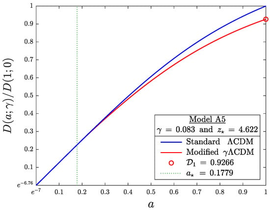
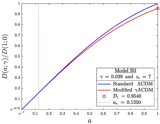
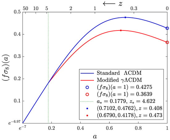
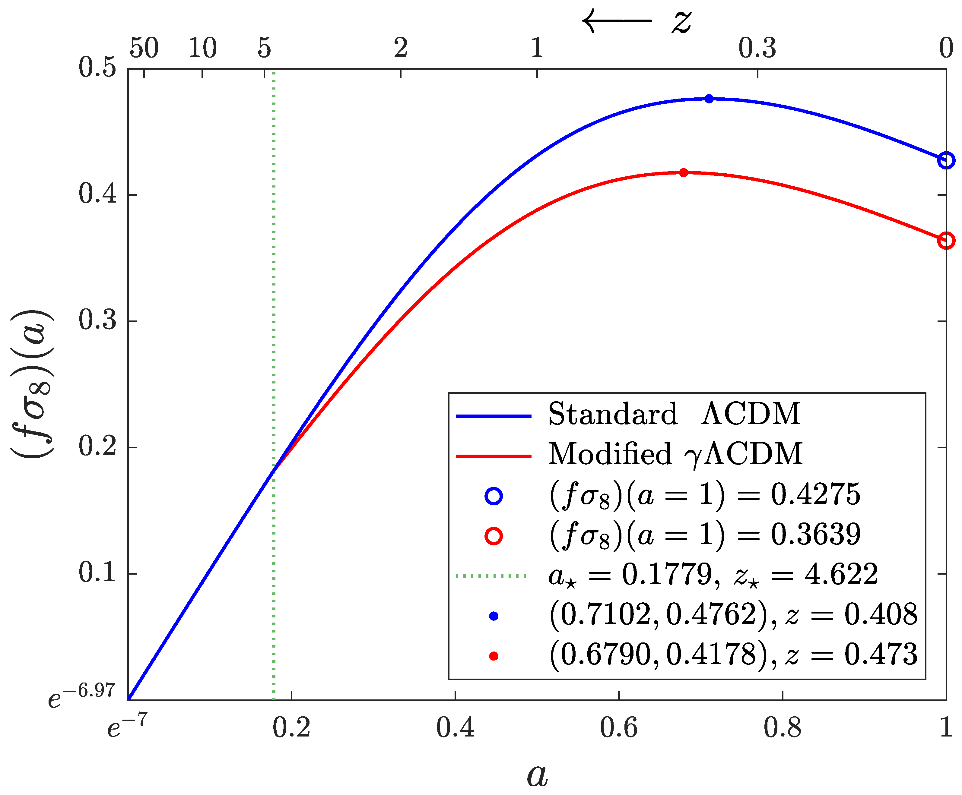
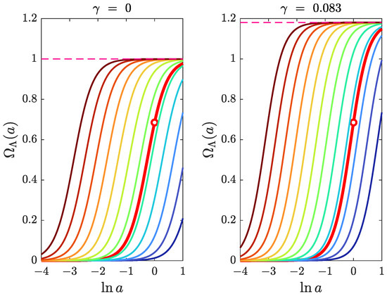
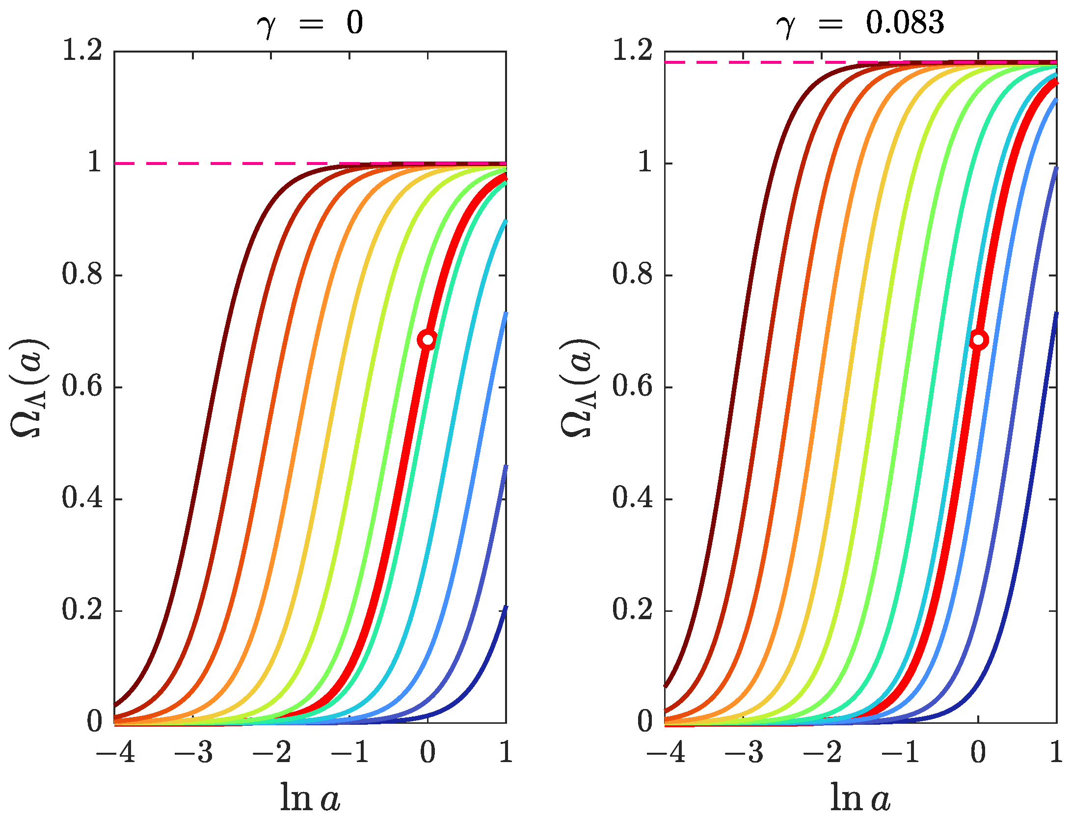
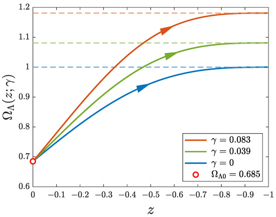
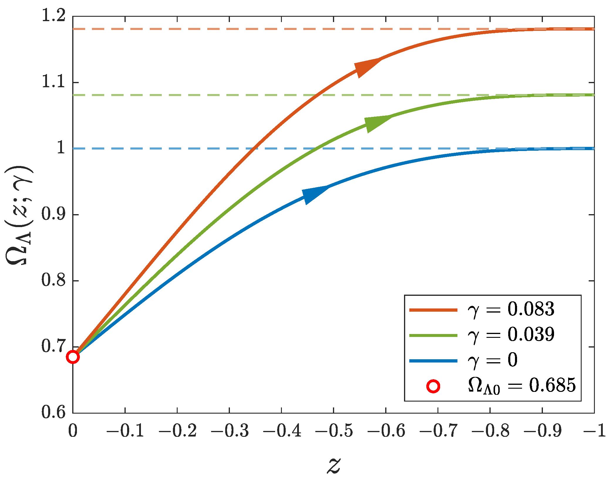
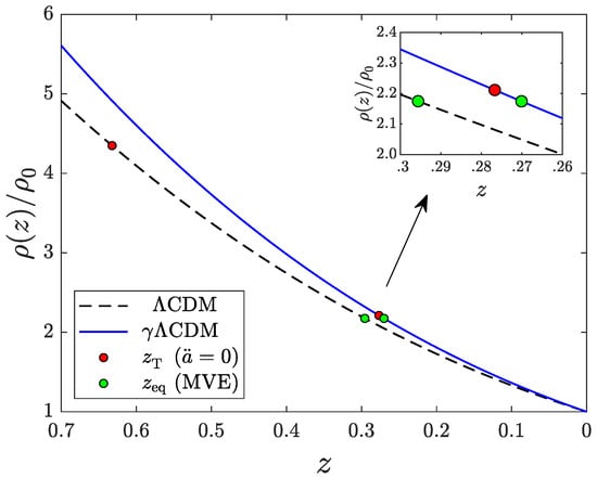
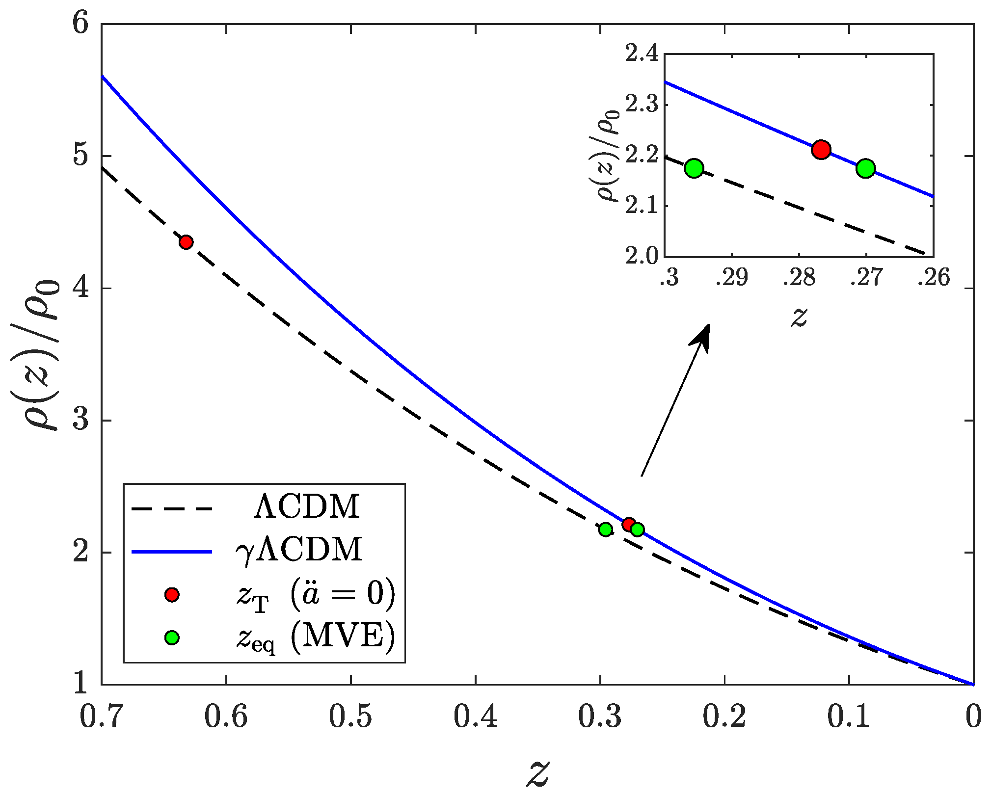
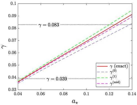
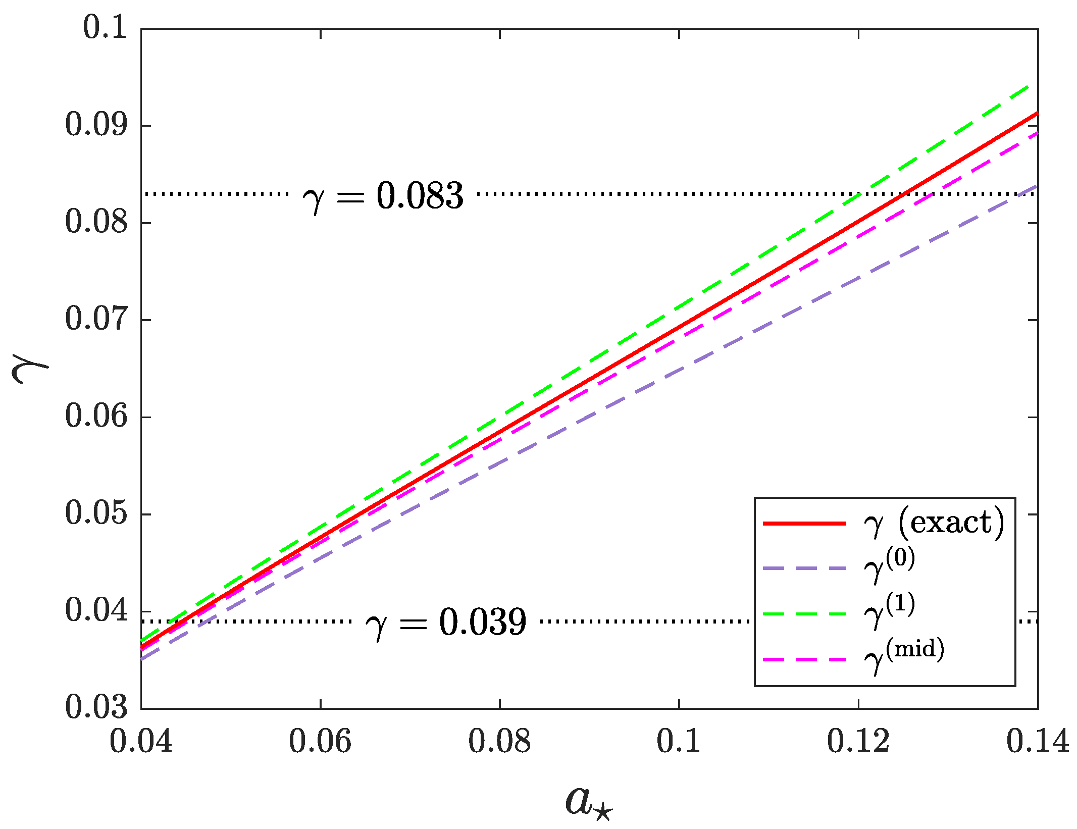

Disclaimer/Publisher’s Note: The statements, opinions and data contained in all publications are solely those of the individual author(s) and contributor(s) and not of MDPI and/or the editor(s). MDPI and/or the editor(s) disclaim responsibility for any injury to people or property resulting from any ideas, methods, instructions or products referred to in the content. |
© 2026 by the authors. Licensee MDPI, Basel, Switzerland. This article is an open access article distributed under the terms and conditions of the Creative Commons Attribution (CC BY) license.