ADP-Based Event-Triggered Optimal Control of Grid-Connected Voltage Source Inverters

Abstract

In this paper, an event-triggered optimal control strategy is proposed for three-phase grid-connected voltage source inverters (VSIs) based on the voltage-modulated direct power control (VM-DPC) principle. The optimization control problem of VSIs is addressed in the framework of nonzero sum (NZS) games to ensure mutual cooperation between active power and reactive power. To achieve optimal performance, the power components are driven to track their desired references while minimizing the individual performance index function. Accurate tracking of active and reactive powers not only stabilizes the grid but also guarantees compliant renewable integration. An adaptive dynamic programming (ADP) approach is adopted, where the critic neural network (NN) approximates the value function and provides optimal control policies. Moreover, an event-triggered mechanism with a dead-zone operation is incorporated to reduce redundant updates, thereby saving computational and communication resources. The stability of the closed-loop system and a strictly positive minimum inter-event interval are guaranteed. Simulation results verify that the proposed method achieves accurate power tracking, improved dynamic performance, and efficient implementation.

1. Introduction

With the rapid development of renewable energy, such as photovoltaic generation, wind power, and battery energy storage, power electronic converters have become indispensable in modern power systems. Unlike traditional synchronous generators, renewable sources cannot be directly interfaced with the grid and therefore rely on converters to regulate power exchange and ensure stable operation. Among various topologies, the grid-connected voltage source inverter (VSI) has emerged as a core interface, enabling the conversion of DC energy into controllable AC power and supporting a wide range of applications including distributed generation [1,2], microgrids [3], and energy storage systems [4].

The dynamic behavior of grid-connected VSIs is principally governed by their control, making their impedance characteristics highly dependent on the chosen control strategy. Common strategies include vector current control (VCC) and direct power control (DPC). In VCC, the inverter output currents are regulated in the synchronous $dq$-frame by means of proportional–integral (PI) controllers and a phase-locked loop (PLL) to synchronize with the grid voltage [5]. This approach offers accurate steady-state performance and is widely adopted in grid-connected converters. However, VCC requires a well-tuned PLL, which may deteriorate performance in weak or distorted grids, and its cascaded structure involving inner current loops and outer voltage loops limits dynamic response.

To overcome these limitations, direct power control (DPC) was proposed to directly regulate instantaneous active and reactive powers, thereby eliminating the need for multiple cascaded loops and enhancing transient dynamics [6,7]. This technique operates without the phase-locked loop (PLL) and achieves low steady-state harmonic distortion through pulse-width modulation (PWM) with a fixed switching frequency. Among various DPC methods, voltage-modulated direct power control (VM-DPC) in the $\alpha \beta$-frame, initially developed for converters, has gained significant attention [8,9,10]. The VM-DPC transforms the original nonlinear time-varying system in a stationary $\alpha \beta$-frame to a linear time-invariant (LTI) system in asynchronous rotating $dq$-frame without PLL and dynamic information loss.

Building on the aforementioned research, this work formulates the VM-DPC model of the grid-connected VSI as a two-input nonlinear dynamic system, where active and reactive powers are treated as the state variables. Since the two control inputs simultaneously influence the system dynamics rather than exhibiting a strictly antagonistic relationship, the problem is naturally modeled as a nonzero-sum game (NZS). For NZS game methods, investigating the Nash equilibrium among multiple agents enables them to coordinate their strategies toward a global optimal outcome. This formulation enables the application of optimal control strategies to achieve cooperative optimization of active and reactive power control, leading to enhanced dynamic performance and adaptability.

In summary, VM-DPC has emerged as a representative benchmark for advanced power control strategies in grid-connected converters. Numerous studies have further extended VM-DPC by integrating various auxiliary control techniques, thereby offering diverse perspectives for performance enhancement. Among these techniques, the proportional–integral scheme is extensively used because of its straightforward structure and reliable performance. Nevertheless, the conventional PI control inherently relies on fixed gains and linear error correction, which limits its ability to achieve optimal performance across different operating conditions and restricts the dynamic enhancement potential of VM-DPC. Moreover, model predictive control (MPC) has also been proposed to enhance the performance of VM-DPC [11,12]. Nonetheless, MPC operates in the discrete domain and requires online linearization and optimization each cycle, which increases computational load and complicates embedded implementation. To further enhance optimization performance, linear quadratic regulator (LQR) has been applied to the VM-DPC framework with finite or infinite horizon optimization [8]. However, the above optimal control approaches typically rely on accurate models, which may reduce their effectiveness in dealing with nonlinear dynamics and time-varying disturbances.

As one of the most effective algorithms to address optimization problems, adaptive dynamic programming (ADP) has found prosperous applications in many systems theoretically and practically, such as grid-connected inverters [13,14], switched systems [15,16] and microgrids [17,18]. By integrating dynamic programming, NNs and reinforcement learning (RL), ADP methods are dedicated to seeking the approximate optimal solution directly, and can get out of the “curse of dimensionality” [19,20]. As for the grid-connected VSIs subject to changing environments and complex system dynamics, the introduction of ADP-based control methods can circumvent the difficulty in obtaining the analytical optimal solution.

Accounting for the bandwidth limitation, frequent control updates and data transmission can bring extra challenges to the optimal control of grid-connected VSIs under the conventional time-triggered mechanism. By employing event-triggered control, the control signal is updated only when necessary or when significant events occur according to a predefined triggering condition. This not only guarantees the stable operation of the VSI system, but also reduces computational complexity and communication burden [20,21]. Therefore, it is of great value to design reliable event-triggered control schemes for grid-connected VSIs.

Inspired by the above, this work combines ADP technologies with event-triggered control to address the optimal control problem of grid-connected VSIs, which is further formulated as a nonzero-sum game. The objective is to ensure that both active and reactive powers accurately track their desired values. Furthermore, such regulation contributes to maintaining grid stability and enables compliant integration of DC sources such as renewable energy units. The main contributions of this article are summarized as follows.

• To the best of our knowledge, this work is the first time an ADP-based algorithm is applied to address the NZS game problem of grid-connected voltage source inverters. By analyzing the Nash equilibrium of active and reactive power interactions, the proposed method enables these power components to collaborate effectively, achieving a globally optimized performance.
• In order to release communication and calculation burdens, a novel group of event-triggered control schemes is devised; meanwhile, the stability of the controlled system is guaranteed.
• The theoretical analysis determines the minimum triggering interval of the proposed mechanism, theoretically ensuring the exclusion of Zeno behavior. Moreover, the introduction of the dead-zone operation leads to the reduction in trigger frequency and the alleviation of communication and calculation burdens.

2. System Model Description and Problem Formulation

In this section, the structure of VSI is briefly introduced, and then the VSI system is formulated by VM-DPC method.

2.1. Modeling of Grid-Connected VSIs

Figure 1 illustrates the topology of a three-phase VSI, where a DC source—representing renewable generation units or energy storage systems—is connected to the grid through an R–L output filter. By applying the Clark transformation, the system dynamics can be formulated in the $\alpha \beta$-frame as a second-order model.

$$\begin{array}{cc}\hfill u_{\alpha }& =R{i}_{\alpha }+L{\displaystyle \frac{d{i}_{\alpha }}{dt}}+v_{g\alpha },\hfill \\ \hfill u_{\beta }& =R{i}_{\beta }+L{\displaystyle \frac{d{i}_{\beta }}{dt}}+v_{g\beta },\hfill \end{array}$$

(1)

where $i_{\alpha \beta }$, $u_{\alpha \beta }$, and $v_{g\alpha \beta }$ represent the output currents and voltages of VSI, and the grid voltages in $\alpha \beta$-frame, respectively. L and R are the inductance and resistance of the filter.

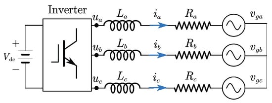
Figure 1. Three-phase voltage source inverter connected to a grid.

The output instantaneous active and reactive power could be described as:

$$\begin{array}{cc}\hfill P& ={\displaystyle \frac{3}{2}}\left(v_{g\alpha }{i}_{\alpha }+v_{g_{\beta }}{i}_{\beta }\right),\hfill \\ \hfill Q& ={\displaystyle \frac{3}{2}}\left(v_{g_{\beta }}{i}_{\alpha }-v_{g\alpha }{i}_{\beta }\right),\hfill \end{array}$$

(2)

where P and Q are the instantaneous active power and reactive power, respectively. The time derivative of (2) is:

$$\begin{array}{cc}\hfill {\displaystyle \frac{dP}{dt}}& ={\displaystyle \frac{3}{2}}\left(i_{\alpha }{\displaystyle \frac{d{v}_{g\alpha }}{dt}}+v_{g\alpha }{\displaystyle \frac{d{i}_{\alpha }}{dt}}+i_{\beta }{\displaystyle \frac{d{v}_{g_{\beta }}}{dt}}+v_{g_{\beta }}{\displaystyle \frac{d{i}_{\beta }}{dt}}\right),\hfill \\ \hfill {\displaystyle \frac{dQ}{dt}}& ={\displaystyle \frac{3}{2}}\left(i_{\alpha }{\displaystyle \frac{d{v}_{g_{\beta }}}{dt}}+v_{g_{\beta }}{\displaystyle \frac{d{i}_{\alpha }}{dt}}-i_{\beta }{\displaystyle \frac{d{v}_{g\alpha }}{dt}}-v_{g\alpha }{\displaystyle \frac{d{i}_{\beta }}{dt}}\right).\hfill \end{array}$$

(3)

Assumption 1.

The grid is considered ideal with balanced and sinusoidal voltages of constant amplitude $V_g$ and angular frequency ω.

In $\alpha \beta$-frame, grid voltages are modeled as

$$\begin{array}{cc}\hfill v_{g\alpha }& =V_g\cos \left(\omega t\right),\hfill \\ \hfill v_{g_{\beta }}& =V_g\sin \left(\omega t\right),\hfill \end{array}$$

(4)

where $V_g$ and $\omega$ denote the grid voltage magnitude and angular frequency. Accordingly, one obtains the following equations:

$$\begin{array}{cc}\hfill {\displaystyle \frac{d{v}_{g\alpha }}{dt}}& =-\omega V_g\sin \left(\omega t\right)=-\omega v_{g_{\beta }},\hfill \\ \hfill {\displaystyle \frac{d{v}_{g_{\beta }}}{dt}}& =\omega V_g\cos \left(\omega t\right)=\omega v_{g\alpha }.\hfill \end{array}$$

(5)

By substituting (2) and (5) into (3), one obtains

$$\begin{array}{ccc}\hfill {\displaystyle \frac{dP}{dt}}& \hfill =& -{\displaystyle \frac{R}{L}}P-\omega Q+{\displaystyle \frac{3}{2L}}\left(v_{g\alpha }{u}_{\alpha }+v_{g_{\beta }}{u}_{\beta }-V_g^2\right),\hfill \\ \hfill {\displaystyle \frac{dQ}{dt}}& \hfill =& \omega P-{\displaystyle \frac{R}{L}}Q+{\displaystyle \frac{3}{2L}}\left(v_{g_{\beta }}{u}_{\alpha }-v_{g\alpha }{u}_{\beta }\right).\hfill \end{array}$$

(6)

At this stage, the dynamics of the real and reactive powers for grid-connected VSIs have been derived. In the following section, these equations are reformulated into a linear time-invariant form based on the VM-DPC principle.

2.2. State-Space Formulation via VM-DPC

It should be noted that due to the time-varying nature of $v_{g\alpha }$ and $v_{g\beta }$, system (6) is a nonlinear time-varying model. The complexity of this structure makes controller design challenging. By employing the VM principle, however, system (6) can be reformulated as a linear time invariant (LTI) model through the introduction of the following two new VM inputs [9].

$$\begin{array}{cc}\hfill u_{VM1}& =v_{g\alpha }{u}_{\alpha }+v_{g_{\beta }}{u}_{\beta },\hfill \\ \hfill u_{VM2}& =v_{g_{\beta }}{u}_{\alpha }-v_{g\alpha }{u}_{\beta }.\hfill \end{array}$$

(7)

Therefore, the model (6) can be transformed as:

$$\begin{array}{cc}\hfill {\displaystyle \frac{dP}{dt}}& =-{\displaystyle \frac{R}{L}}P-\omega Q-{\displaystyle \frac{3}{2L}}{V}_g^2+{\displaystyle \frac{3}{2L}}{u}_{VM1},\hfill \\ \hfill {\displaystyle \frac{dQ}{dt}}& =\omega P-{\displaystyle \frac{R}{L}}Q+{\displaystyle \frac{3}{2L}}{u}_{VM2}.\hfill \end{array}$$

(8)

This study investigates power tracking control for grid-connected VSIs, where the active and reactive powers are regulated to their references $P_{\mathrm{ref}}$ and $Q_{\mathrm{ref}}$, thereby maintaining grid frequency and voltage stability while ensuring compliant interconnection. Based on the VM-DPC formulation, the steady-state relations between the power dynamics and the control inputs can be obtained by enforcing the equilibrium conditions $dP/dt=0$ and $dQ/dt=0$. Consequently, the inputs $u_{VM1}$ and $u_{VM2}$ strive to reach their corresponding steady-state references $u_{VM1}^{*}$ and $u_{VM2}^{*}$, which can be explicitly derived from $P_{\mathrm{ref}}$ and $Q_{\mathrm{ref}}$ as

$$\begin{array}{cc}\hfill u_{VM1}^{*}& ={\displaystyle \frac{2L}{3}}\left({\displaystyle \frac{R}{L}}{P}_{\mathrm{ref}}+\omega Q_{\mathrm{ref}}+{\displaystyle \frac{3}{2L}}{V}_g^2\right),\hfill \\ \hfill u_{VM2}^{*}& ={\displaystyle \frac{2L}{3}}\left({\displaystyle \frac{R}{L}}{Q}_{\mathrm{ref}}-\omega P_{\mathrm{ref}}\right).\hfill \end{array}$$

(9)

At the same time, the overall system is reformulated into a state-space form that provides the basis for subsequent optimal control design.

Since the active and reactive power loops pursue different performance objectives and impose mutually coupled effects through the converter dynamics, their regulation naturally forms a two-player nonzero-sum interaction. Modeling the control as an NZS game enables deriving equilibrium control policies that balance both channels in an optimal and coordinated manner.

Design the error state as $x\left(t\right)={\left[P\left(t\right)-P_{\mathrm{ref}},Q\left(t\right)-Q_{\mathrm{ref}}\right]}^T$ and the corresponding control input as $u_1\left(t\right)=u_{VM1}-u_{VM1}^{*}$, $u_2\left(t\right)=u_{VM2}-u_{VM2}^{*}$. Then, the model of the grid-connected VSIs is deduced as follows:

$$\begin{array}{cc}\hfill \dot{x}\left(t\right)& =\left[\begin{array}{cc}-{\displaystyle \frac{R}{L}}& -\omega \\ \omega & -{\displaystyle \frac{R}{L}}\end{array}\right]x\left(t\right)+\left[\begin{array}{c}{\displaystyle \frac{3}{2L}}\\ 0\end{array}\right]u_1\left(t\right)+\left[\begin{array}{c}0\\ {\displaystyle \frac{3}{2L}}\end{array}\right]u_2\left(t\right)\hfill \\ \hfill & =f\left(x\right)+\sum _{j=1}^2{g}_j{u}_j,\hfill \end{array}$$

(10)

with $f\left(x\right)=\left[\begin{array}{cc}-{\displaystyle \frac{R}{L}}& -\omega \\ \omega & -{\displaystyle \frac{R}{L}}\end{array}\right]x\left(t\right)$, $g_1=\left[\begin{array}{c}{\displaystyle \frac{3}{2L}}\\ 0\end{array}\right]$ and $g_2=\left[\begin{array}{c}0\\ {\displaystyle \frac{3}{2L}}\end{array}\right]$.

Remark 1.

Compared to traditional decoupled control or centralized optimal control [8,11,12], the proposed game-theoretic framework explicitly captures the coupling between the P–Q dynamics and the mutual influence between their individual regulation objectives. This enables the two control input to independently adjust their strategies based on their own performance index while still achieving cooperative optimization through the Nash equilibrium.

3. Event-Triggered Adaptive Critic Design

This part introduces an ET-driven ADP framework designed to solve the NZS game problem of the grid-connected VSI system (10). The proposed approach ensures efficient power regulation while reducing computational load. Furthermore, the stability of the closed-loop system is rigorously analyzed.

Figure 2 block diagram of the proposed event-triggered ADP control scheme. The system states are sampled and sent to the ET-ADP controller, where the critic neural network and weight-update law approximate the Hamilton function and compute the optimal control policy. An event-triggering mechanism determines control updates, and the resulting input is applied to the actuator to close the loop.

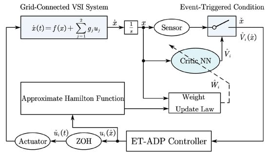
Figure 2. Structure diagram of the proposed control scheme.

3.1. Triggering Adaptive Controller Design

First of all, to capture the interactions between the active and reactive power regulation objectives in the grid-connected VSI system, the control problem is formulated as an NZS differential game. The performance index corresponding to the ith decision maker is written as

$$\begin{array}{c}\hfill J_i\left(x\left(0\right)\right)={\int }_0^{\infty }\left(x^T{Q}_{i}x+{\mathcal{W}}_i\left(u_i\right)\right)d\tau \triangleq {\int }_0^{\infty }{v}_i(x,u_{r1},u_{r2})d\tau ,\end{array}$$

(11)

where $i=1,2$ and $Q_1,Q_2\in {\mathbb{R}}^{2\times 2}$ are symmetric and positive definite. Following the formulation in [22], the input-related cost components ${\mathcal{W}}_1\left(u_1\right)$ and ${\mathcal{W}}_2\left(u_2\right)$ are given by

$$\begin{array}{c}\hfill {\mathcal{W}}_1\left(u_1\right)=u_1^T{R}_{11}{u}_1+u_2^T{R}_{12}{u}_1,\end{array}$$

(12)

$$\begin{array}{c}\hfill {\mathcal{W}}_2\left(u_2\right)=u_1^T{R}_{21}{u}_1+u_2^T{R}_{22}{u}_2,\end{array}$$

(13)

where $R_{ij}$$(i,j=1,2)$ denote the corresponding weighting matrices. Accordingly, the value function associated with the ith player is represented as

$$\begin{array}{c}\hfill V_i\left(x\left(t\right)\right)={\int }_t^{\infty }\left(x^T{Q}_{i}x+{\mathcal{W}}_i\left(u_i\right)\right)d\tau .\end{array}$$

(14)

Definition 1

([19,23]). A pair of control strategies $\{u_1^{*},u_2^{*}\}$ is regarded as a Nash equilibrium if

$$\begin{array}{c}\hfill V_1(u_1^{*},u_2^{*})\le V_1(u_1^{*},u_2),\end{array}$$

(15)

$$\begin{array}{c}\hfill V_2(u_1^{*},u_2^{*})\le V_2(u_1,u_2^{*})\end{array}$$

(16)

hold for every admissible $u_1$ and $u_2$. That is, neither player can improve its own performance index through unilateral deviation from $u_i^{*}$.

The Hamiltonian corresponding to the ith player under the admissible control policies can be written as

$$\begin{array}{cc}\hfill H_i& =x^T{Q}_{i}x+{\mathcal{W}}_i\left(u_i\right)\hfill \\ \hfill & +{(\nabla V_i)}^T\left(f\left(x\right)+\sum _{j=1}^2{g}_j\left(x\right)u_j\left(x\right)\right),\hfill \end{array}$$

(17)

where $j=1,2$, and $\nabla V_i\in {\mathbb{R}}^2$ denotes the gradient of $V_i$ with respect to the state vector x.

Thus, the optimal value function

$$\begin{array}{c}\hfill V_i^{*}\left(x\left(t\right)\right)=\underset{u_{ri}}{min}\left\{{\int }_t^{\infty }(x^T{Q}_{i}x+{\mathcal{W}}_i\left(u_i\right))d\tau \right\}\end{array}$$

(18)

satisfies the HJ equation

$$\begin{array}{c}\hfill \underset{u_i}{min}{H}_i(x,u_1,u_2,V_i^{*})=0.\end{array}$$

(19)

From the stationarity property of the HJ equation, the optimal control inputs for the two players are obtained as

$$\begin{array}{c}\hfill u_1^{*}=-{\displaystyle \frac{1}{2}}{R}_{11}^{-1}{g}_1^T\left(x\right)\nabla V_1^{*},\end{array}$$

(20)

$$\begin{array}{c}\hfill u_2^{*}=-{\displaystyle \frac{1}{2}}{R}_{22}^{-1}{g}_2^T\left(x\right)\nabla V_2^{*}.\end{array}$$

(21)

Owing to the difficulty and complexity of directly solving the HJ equation, the optimal value function $V_i^{*}$ is approximated through a critic neural network as

$$\begin{array}{c}\hfill V_i^{*}=W_i^{*T}{\sigma }_i\left(x\right)+{\epsilon }_i,\end{array}$$

(22)

where $W_i^{*}\in {\mathbb{R}}^L$ denotes the ideal weight vector, ${\sigma }_i\left(x\right)\in {\mathbb{R}}^L$ is the selected activation basis, L represents the number of neurons in the hidden layer, and ${\epsilon }_i$ stands for the residual approximation term.

Since the ideal critic-network weight $W_i^{*}$ is unavailable in practice, (22) cannot be directly utilized. Let ${\widehat{W}}_i$ denote the adaptive estimate of $W_i^{*}$. Accordingly, the critic NN output is taken as

$$\begin{array}{c}\hfill {\widehat{V}}_i={\widehat{W}}_i^T{\sigma }_i\left(x\right).\end{array}$$

(23)

Furthermore, differentiating $V_i^{*}$ with respect to x yields

$$\begin{array}{c}\hfill \nabla V_i^{*}={(\nabla {\sigma }_i\left(x\right))}^T{W}_i^{*}+\nabla {\epsilon }_i.\end{array}$$

(24)

Similarly, we have

$$\begin{array}{c}\hfill \nabla {\widehat{V}}_i={(\nabla {\sigma }_i\left(x\right))}^T{\widehat{W}}_i.\end{array}$$

(25)

By substituting (24) into (20)–(21), the ADP-based optimal control laws are expressed as

$$u_1^{*}=-\frac{1}{2}{R}_{11}^{-1}{g}_1^T\left(x\right)\left(\nabla {\sigma }_1{\left(x\right)}^T{W}_1^{*}+\nabla {\epsilon }_1\right),$$

(26)

$$u_2^{*}=-\frac{1}{2}{R}_{22}^{-1}{g}_2^T\left(x\right)\left(\nabla {\sigma }_2{\left(x\right)}^T{W}_2^{*}+\nabla {\epsilon }_2\right).$$

(27)

Let ${\left\{z_k\right\}}_{k=0}^{\infty }$ denote the sequence of event-triggering instants, where $z_k$ is the k-th sampling time. The state is held constant between two consecutive sampling times, i.e., ${\check{x}}_k=x\left(z_k\right)$ for $z_k\le t<z_{k+1}$. Using a zero-order holder, the control inputs become

$$\begin{array}{c}\hfill {\check{u}}_1\left(t\right)=u_1({\check{x}}_k,t),{\check{u}}_2\left(t\right)=u_2({\check{x}}_k,t),z_k\le t<z_{k+1}.\end{array}$$

(28)

Define the measurement error as ${\pi }_l=x\left(t\right)-{\check{x}}_k$, $z_k\le t<z_{k+1}$. Replacing $W_i^{*}$ with its adaptive estimate ${\widehat{W}}_i\left(z_k\right)$ and evaluating the controller at the sampled state ${\check{x}}_k$, the implementable control laws are given by

$${\check{u}}_1=-\frac{1}{2}{R}_{11}^{-1}{g}_1^T\left({\check{x}}_k\right){\left(\nabla {\sigma }_1\left({\check{x}}_k\right)\right)}^T{\widehat{W}}_1\left(z_k\right),$$

(29)

$${\check{u}}_2=-\frac{1}{2}{R}_{22}^{-1}{g}_2^T\left({\check{x}}_k\right){\left(\nabla {\sigma }_2\left({\check{x}}_k\right)\right)}^T{\widehat{W}}_2\left(z_k\right).$$

(30)

Based on the above controller representation, the Hamiltonian residual for the ith player is written as

$$\begin{array}{cc}\hfill & H_i\left(x,{\check{u}}_1,{\check{u}}_2,{\widehat{W}}_i\right)\hfill \\ \hfill =& x^T{Q}_{i}x+\mathcal{W}\left({\check{u}}_i\right)+{\widehat{W}}_i^T\nabla {\sigma }_i\dot{x}\hfill \\ \hfill =& x^T{Q}_{i}x+\mathcal{W}\left({\check{u}}_i\right)+{\widehat{W}}_i^T{\hslash }_i\hfill \\ \hfill \stackrel{\Delta }{=}& e_i.\hfill \end{array}$$

(31)

We introduced an auxiliary term as

$$\begin{array}{cc}\hfill & H_i(x,{\check{u}}_1,{\check{u}}_2,W_i^{*})\hfill \\ \hfill =& x^T{Q}_{i}x+\mathcal{W}\left({\check{u}}_i\right)+W_i^{*T}{\hslash }_i\hfill \\ \hfill \stackrel{\Delta }{=}& {\epsilon }_{H_i}.\hfill \end{array}$$

(32)

To reduce the Hamiltonian residual $e_i$, the critic weights ${\widehat{W}}_i$ are adjusted to minimize the performance index

$$\begin{array}{c}\hfill \kappa \triangleq \sum _{i=1}^2{\kappa }_i={\displaystyle \frac{1}{2}}\sum _{i=1}^2{e}_i^2.\end{array}$$

(33)

Applying the gradient descent method [24], the weight update law for the ith critic network is obtained as

$$\begin{array}{cc}\hfill {\dot{\widehat{W}}}_i& =-{\iota }_i{\displaystyle \frac{1}{{({\hslash }_i^T{\hslash }_i+1)}^2}}{\displaystyle \frac{\partial \kappa }{\partial {\widehat{W}}_i}}=-{\iota }_i{\displaystyle \frac{1}{{({\hslash }_i^T{\hslash }_i+1)}^2}}{\displaystyle \frac{\partial {\kappa }_i}{\partial {\widehat{W}}_i}}\hfill \\ \hfill & =-{\iota }_i{\displaystyle \frac{{\hslash }_i{e}_i}{{({\hslash }_i^T{\hslash }_i+1)}^2}}=-{\displaystyle \frac{{\iota }_i{\hslash }_i{\epsilon }_{H_i}}{{({\hslash }_i^T{\hslash }_i+1)}^2}}+{\displaystyle \frac{{\iota }_i{\hslash }_i{\hslash }_i^T{\tilde{W}}_i}{{({\hslash }_i^T{\hslash }_i+1)}^2}},\hfill \end{array}$$

(34)

where ${\tilde{W}}_i=W_i^{*}-{\widehat{W}}_i$ is the weight estimation error, and ${\iota }_i>0$ denotes the learning rate. Since $W_i^{*}$ is constant, it follows that

$$\begin{array}{c}\hfill {\dot{\tilde{W}}}_i=-{\dot{\widehat{W}}}_i={\displaystyle \frac{{\iota }_i{\hslash }_i{\epsilon }_{H_i}}{{({\hslash }_i^T{\hslash }_i+1)}^2}}-{\displaystyle \frac{{\iota }_i{\hslash }_i{\hslash }_i^T{\tilde{W}}_i}{{({\hslash }_i^T{\hslash }_i+1)}^2}}.\end{array}$$

(35)

3.2. Event-Based Adaptive Critic Design and Stability Analysis

For the subsequent stability analysis, we adopt the following assumptions as in [22,25].

Assumption 2.

The control law satisfies a Lipschitz condition, i.e.,

$$\begin{array}{c}\hfill \parallel u_j^{*}\left(x\right)-u_j^{*}\left({\check{x}}_k\right){\parallel }^2\le {\varpi }_j\parallel x-{\check{x}}_k{\parallel }^2={\varpi }_j{\parallel {\pi }_l\parallel }^2,z_k\le t<z_{k+1},\end{array}$$

(36)

where ${\varpi }_j>0$.

Assumption 3.

For any $i,j\in 1,2$, the optimal critic NN weight $W_i^{*}$, the input coefficient matrix $g_j\left(x\right)$, the partial derivative of the NN activation function $\nabla {\sigma }_i$, the partial derivative of the NN estimation error $\nabla {\epsilon }_i$ and the additional term ${\epsilon }_{H_i}$ are norm bounded, that is $\left|\right|g_j\left(x\right)\left|\right|\le {\overline{\mathcal{G}}}_j,\left|\right|W_i^{*}\left|\right|\le c_{{\overline{W}}_i},\left|\right|\nabla {\sigma }_i\left|\right|\le {\overline{\sigma }}_i,\left|\right|\nabla {\epsilon }_i\left|\right|\le {\overline{\epsilon }}_i,{\epsilon }_{H_i}\le \overline{{\epsilon }_{H_i}},$ where ${\overline{\mathcal{G}}}_j$, $c_{{\overline{W}}_i}$, ${\overline{\sigma }}_i$, ${\overline{\epsilon }}_i$ and $\overline{{\epsilon }_{H_i}}$ are all positive constants.

Assumption 4.

Under the persistence of excitation (PE) condition, the signal ${\underline{\hslash }}_i$ of each player remains persistently excited, which guarantees the following inequality:

$$\begin{array}{c}\hfill {\mathcal{H}}_i\mathcal{F}\le {\int }_t^{t+T}{\underline{\hslash }}_i{\underline{\hslash }}_i^{T}d\tau ,\end{array}$$

(37)

where ${\underline{\hslash }}_i={\displaystyle \frac{{\hslash }_i}{{\hslash }_i^T{\hslash }_i+1}}$, and ${\mathcal{H}}_i$, $\mathcal{F}$ are positive constants. The inequality implies that $0<{\mathcal{H}}_i\le {\lambda }_{min}\left({\underline{\hslash }}_i{\underline{\hslash }}_i^T\right)$.

Lemma 1.

Suppose that the above assumptions all hold. For the grid-connected VSI model (10), using the event-triggered control strategy (29), (30) and the adaptive law of the critic NN weight (34), there exists $T_l>0$, such that when $t>T_l$, the weight estimation error of the critic NN, i.e., ${\tilde{W}}_i$, is uniformly ultimately bounded (UUB).

Proof. 

To analyze the stability of the weight estimation error ${\tilde{W}}_i$, consider the Lyapunov function as

$$\mathcal{J}=\sum _{i=1}^2{\tilde{W}}_i^T{\tilde{W}}_i.$$

(38)

Since the dynamics of ${\tilde{W}}_i$ evolve according to a continuous flow and ${\tilde{W}}_i$ is continuous in time over the interval $[0,+\infty )$, it follows that the first-order difference of $\mathcal{J}$ at the triggering instant $t=z_k$ satisfies $\Delta \mathcal{J}=0.$

Therefore, it is sufficient to analyze the behavior of the system during the flow period.

For $t\in [z_k,z_{k+1})$, we obtain

$$\begin{array}{cc}\hfill \dot{\mathcal{J}}=& 2{\iota }_i{\tilde{W}}_i^T\left({\displaystyle \frac{{\underline{\hslash }}_i{\epsilon }_{H_i}}{{\hslash }_i^T{\hslash }_i+1}}-{\displaystyle \frac{{\hslash }_i{\hslash }_i^T}{{\left({\hslash }_i^T{\hslash }_i+1\right)}^2}}{\tilde{W}}_i\right)\hfill \\ \hfill \le & {\iota }_i{\displaystyle \frac{{\epsilon }_{H_i}^2-{\tilde{W}}_i^T{\hslash }_i{\hslash }_i^T{\tilde{W}}_i}{{\left({\hslash }_i^T{\hslash }_i+1\right)}^2}}\hfill \\ \hfill \le & {\iota }_i\left({\overline{{\epsilon }_{H_i}}}^2-{\lambda }_{min}\left({\underline{\hslash }}_i{\underline{\hslash }}_i^T\right){\parallel {\tilde{W}}_i\parallel }^2\right)\hfill \\ \hfill \le & {\iota }_i{\overline{{\epsilon }_{H_i}}}^2-{\iota }_i{\mathcal{H}}_i{\parallel {\tilde{W}}_i\parallel }^2.\hfill \end{array}$$

(39)

Based on Equation (39), this implies that when

$$\parallel {\tilde{W}}_i\parallel >{\displaystyle \frac{\overline{{\epsilon }_{H_i}}}{\sqrt{{\mathcal{H}}_i}}}\triangleq {{\rm Y}}_{{\tilde{W}}_i},$$

(40)

we have $\dot{\mathcal{J}}<0.$

In other words, there exists a constant $T_1>0$ such that, for all $z_k>T_1$, the weight estimation error ${\tilde{W}}_i$ is uniformly ultimately bounded (UUB) by the upper bound ${{\rm Y}}_{{\tilde{W}}_i}$. □

Theorem 1.

For the NZS games formulated in system (10), assume that the approximate optimal control inputs in (29), (30) together with the weight adaptation law in (34) are implemented. Under the following triggering condition:

$$\begin{array}{c}\hfill \Pi \left({\pi }_l\right)\le \sqrt{{\displaystyle \frac{{\alpha }_c{\sum }_{i=1}^2{\lambda }_{min}\left(Q_i\right)}{{\overline{\mathcal{G}}}^2{\sum }_{j=1}^2{\varpi }_j}}}\left|\right|x\left|\right|\stackrel{\Delta }{=}{Z}_T\end{array}$$

(41)

holds, with the dead-zone operation

$$\begin{array}{c}\hfill \Pi \left({\pi }_l\right)=\left\{\begin{array}{cc}\parallel {\pi }_l\parallel ,\hfill & if\parallel x\parallel >\varrho ,\hfill \\ 0,\hfill & if\parallel x\parallel \le \varrho .\hfill \end{array}\right.\end{array}$$

(42)

Here, parameter ${\alpha }_c\in (0,1)$ and the given positive constant ϱ is the triggering termination condition. We define $[g_1\left(x\right),g_2\left(x\right)]{[g_1\left(x\right),g_2\left(x\right)]}^T=\mathcal{G}$ and it is assumed to be bounded as $\parallel \mathcal{G}\parallel \le \overline{\mathcal{G}}$. Then the weight estimation errors ${\tilde{W}}_i$ and the system state x are UUB.

Proof. 

Let Lyapunov function candidate be given by $\mathcal{P}={\mu }_1{\mathcal{P}}_1+{\mu }_2{\mathcal{P}}_2+{\mu }_3{\mathcal{P}}_3,{\mathcal{P}}_1={\sum }_{i=1}^2{V}_i^{*}\left(x\right),{\mathcal{P}}_2={\sum }_{i=1}^2{V}_i^{*}\left({\check{x}}_k\right)+{\sum }_{i=1}^2{\tilde{W}}_i^T\left(z_k\right){\tilde{W}}_i\left(z_k\right),{\mathcal{P}}_3={\sum }_{i=1}^2{\tilde{W}}_i^T{\tilde{W}}_i$.

Case 1. 

When $z_k\le t<z_{k+1}$, the time derivative of ${\mathcal{P}}_1$ is

$$\begin{array}{cc}\hfill {\dot{\mathcal{P}}}_1=& \sum _{i=1}^2{\left(\nabla V_i^{*}\right)}^{T}f\left(x\right)\hfill \\ \hfill & +\sum _{i=1}^2{\left(\nabla V_i^{*}\right)}^T(\sum _{j=1}^2{g}_j(x){\check{u}}_j\left(x\right)).\hfill \end{array}$$

(43)

Due to Equation (19), the following equation holds:

$$\begin{array}{cc}\hfill & \sum _{i=1}^2{\left(\nabla V_i^{*}\right)}^{T}f\left(x\right)\hfill \\ \hfill =& -\sum _{i=1}^2\left(x^T{Q}_{i}x+{\mathcal{W}}_i\left(u_i\right)\right)\hfill \\ \hfill & -\sum _{i=1}^2\left({\left(\nabla V_i^{*}\right)}^T(\sum _{j=1}^2{g}_j(x)u_j^{*}\left(x\right))\right).\hfill \end{array}$$

(44)

Submitting (44) into (43), we can have (45), as shown at the top of next page.

$$\begin{array}{ccc}\hfill {\dot{\mathcal{P}}}_1& =& \sum _{i=1}^2\left(-x^T{Q}_{i}x-{\mathcal{W}}_i\left(u_i\right)\right)+\sum _{i=1}^2{\left(\nabla V_i^{*}\right)}^T\left(\sum _{j=1}^2{g}_j\left(x\right)({\check{u}}_j\left(x\right)-u_j^{*}(x))\right)\hfill \\ \hfill & =& \sum _{i=1}^2\left(-x^T{Q}_{i}x-{\mathcal{W}}_i\left(u_i\right)\right)+{[\nabla V_1^{*}\left(x\right)+\nabla V_2^{*}\left(x\right)]}^T\sum _{j=1}^2{g}_j\left(x\right)({\check{u}}_j\left(x\right)-u_j^{*}\left(x\right))\hfill \\ \hfill & \le & \sum _{i=1}^2\left(-x^T{Q}_{i}x-{\mathcal{W}}_i(u_i)\right)+{\displaystyle \frac{1}{2}}{[\nabla V_1^{*}\left(x\right)+\nabla V_2^{*}\left(x\right)]}^T[\nabla V_1^{*}\left(x\right)+\nabla V_2^{*}\left(x\right)]\hfill \\ \hfill & & +{\displaystyle \frac{1}{2}}{\left[\begin{array}{c}{\check{u}}_1\left(x\right)-u_1^{*}\left(x\right)\\ {\check{u}}_2\left(x\right)-u_2^{*}\left(x\right)\end{array}\right]}^T{[g_1\left(x\right),g_2\left(x\right)]}^T[g_1\left(x\right),g_2\left(x\right)]\left[\begin{array}{c}{\check{u}}_1\left(x\right)-u_1^{*}\left(x\right)\\ {\check{u}}_2\left(x\right)-u_2^{*}\left(x\right)\end{array}\right]\hfill \\ \hfill & \le & \sum _{i=1}^2(-x^T{Q}_{i}x)+\sum _{i=1}^2\parallel \nabla {\sigma }_i{\left(x\right)}^T{W}_i^{*}+\nabla {\epsilon }_i{\parallel }^2+{\displaystyle \frac{1}{2}}{\overline{\mathcal{G}}}^2\sum _{j=1}^2{\parallel {\check{u}}_j\left(x\right)-u_j^{*}\left(x\right)\parallel }^2\hfill \\ \hfill & \le & \sum _{i=1}^2(-x^T{Q}_{i}x)+2\sum _{i=1}^2{\overline{\sigma }}_i^2{c}_{{\overline{W}}_i}^2+2\sum _{i=1}^2{\overline{\epsilon }}_i^2+{\displaystyle \frac{1}{2}}{\overline{\mathcal{G}}}^2\sum _{j=1}^2{\parallel {\check{u}}_j\left(x\right)-u_j^{*}\left(x\right)\parallel }^2\hfill \end{array}$$

(45)

By using Young’s inequality, we further obtain

$$\begin{array}{cc}\hfill & \parallel {\check{u}}_1\left(x\right)-u_1^{*}{\left(x\right)\parallel }^2\hfill \\ \hfill =& \parallel ({\check{u}}_1\left(x\right)-{\check{u}}_1^{*}\left(x\right))+({\check{u}}_1^{*}\left(x\right)-u_1^{*}\left(x\right)){\parallel }^2\hfill \\ \hfill \le & 2\parallel {\check{u}}_1\left(x\right)-{\check{u}}_1^{*}{\left(x\right)\parallel }^2+2{\parallel {\check{u}}_1^{*}\left(x\right)-u_1^{*}\left(x\right)\parallel }^2\hfill \\ \hfill \le & \parallel R_{11}^{-1}{\parallel }^2{\overline{\mathcal{G}}}_1^2({\overline{\sigma }}_1^2{{\rm Y}}_{{\tilde{W}}_1}^2+{\overline{\epsilon }}_1^2)+2{\varpi }_1\left|\right|{\pi }_l{\left|\right|}^2,\hfill \end{array}$$

(46)

$$\begin{array}{cc}\hfill & \parallel {\check{u}}_2\left(x\right)-u_2^{*}{\left(x\right)\parallel }^2\hfill \\ \hfill =& \parallel ({\check{u}}_2\left(x\right)-{\check{u}}_2^{*}\left(x\right))+({\check{u}}_2^{*}\left(x\right)-u_2^{*}\left(x\right)){\parallel }^2\hfill \\ \hfill \le & 2\parallel {\check{u}}_2\left(x\right)-{\check{u}}_2^{*}{\left(x\right)\parallel }^2+2{\parallel {\check{u}}_2^{*}\left(x\right)-u_2^{*}\left(x\right)\parallel }^2\hfill \\ \hfill \le & \parallel R_{22}^{-1}{\parallel }^2{\overline{\mathcal{G}}}_2^2({\overline{\sigma }}_2^2{{\rm Y}}_{{\tilde{W}}_2}^2+{\overline{\epsilon }}_2^2)+2{\varpi }_2\left|\right|{\pi }_l{\left|\right|}^2.\hfill \end{array}$$

(47)

Through the derivation procedure, the subsequent equations can be obtained:

$$\begin{array}{cc}\hfill & \parallel {\check{u}}_1\left(x\right)-{\check{u}}_1^{*}{\left(x\right)\parallel }^2\hfill \\ \hfill =& \left|\right|{\displaystyle \frac{1}{2}}{R}_{11}^{-1}{g}_1^T\left({\check{x}}_k\right){(\nabla {\sigma }_1\left({\check{x}}_k\right))}^T{\widehat{W}}_1\left(z_k\right)\hfill \\ \hfill & -{\displaystyle \frac{1}{2}}{R}_{11}^{-1}{g}_1^T\left({\check{x}}_k\right)\left({(\nabla {\sigma }_1\left({\check{x}}_k\right))}^T{W}_1^{*}\left(z_k\right)+\nabla {\epsilon }_1\right)|{|}^2\hfill \\ \hfill \le & {\displaystyle \frac{1}{4}}\left|\right|R_{11}^{-1}{g}_1^T\left({\check{x}}_k\right){(\nabla {\sigma }_1\left({\check{x}}_k\right))}^T{\widehat{W}}_1\left(z_k\right)\hfill \\ \hfill & -R_{11}^{-1}{g}_1^T\left({\check{x}}_k\right)\left({(\nabla {\sigma }_1\left({\check{x}}_k\right))}^T{W}_1^{*}\left(z_k\right)+\nabla {\epsilon }_1\right)|{|}^2\hfill \\ \hfill \le & {\displaystyle \frac{1}{4}}\parallel R_{11}^{-1}{\parallel }^2\parallel g_1^T\left({\check{x}}_k\right){\parallel }^2{\Vert -{(\nabla {\sigma }_1\left({\check{x}}_k\right))}^T{\tilde{W}}_1\left(z_k\right)-\nabla {\epsilon }_1\parallel }^2\hfill \\ \hfill \le & {\displaystyle \frac{1}{2}}{\parallel R_{11}^{-1}\parallel }^2{\overline{\mathcal{G}}}_1^2({\overline{\sigma }}_1^2{{\rm Y}}_{{\tilde{W}}_1}^2+{\overline{\epsilon }}_1^2),\hfill \end{array}$$

(48)

$$\begin{array}{cc}\hfill & \parallel {\check{u}}_2\left(x\right)-{\check{u}}_2^{*}{\left(x\right)\parallel }^2\hfill \\ \hfill =& \left|\right|{\displaystyle \frac{1}{2}}{R}_{22}^{-1}{g}_2^T\left({\check{x}}_k\right){(\nabla {\sigma }_2\left({\check{x}}_k\right))}^T{\widehat{W}}_2\left(z_k\right)\hfill \\ \hfill & -{\displaystyle \frac{1}{2}}{R}_{22}^{-1}{g}_2^T\left({\check{x}}_k\right)\left({(\nabla {\sigma }_2\left({\check{x}}_k\right))}^T{W}_2^{*}\left(z_k\right)+\nabla {\epsilon }_2\right)|{|}^2\hfill \\ \hfill \le & {\displaystyle \frac{1}{4}}\left|\right|R_{22}^{-1}{g}_2^T\left({\check{x}}_k\right){(\nabla {\sigma }_2\left({\check{x}}_k\right))}^T{\widehat{W}}_2\left(z_k\right)\hfill \\ \hfill & -R_{22}^{-1}{g}_2^T\left({\check{x}}_k\right)\left({(\nabla {\sigma }_2\left({\check{x}}_k\right))}^T{W}_2^{*}\left(z_k\right)+\nabla {\epsilon }_2\right)|{|}^2\hfill \\ \hfill \le & {\displaystyle \frac{1}{4}}\parallel R_{22}^{-1}{\parallel }^2\parallel g_2^T\left({\check{x}}_k\right){\parallel }^2{\Vert -{(\nabla {\sigma }_2\left({\check{x}}_k\right))}^T{\tilde{W}}_2\left(z_k\right)-\nabla {\epsilon }_1\parallel }^2\hfill \\ \hfill \le & {\displaystyle \frac{1}{2}}{\parallel R_{22}^{-1}\parallel }^2{\overline{\mathcal{G}}}_1^2({\overline{\sigma }}_2^2{{\rm Y}}_{{\tilde{W}}_2}^2+{\overline{\epsilon }}_2^2).\hfill \end{array}$$

(49)

Submitting (46)–(49) into (45), it yields that

$$\begin{array}{cc}\hfill {\dot{\mathcal{P}}}_1\le & \sum _{i=1}^2(-x^T{Q}_{i}x)+2\sum _{i=1}^2{\overline{\sigma }}_i^2{c}_{{\overline{W}}_i}^2+2\sum _{i=1}^2{\overline{\epsilon }}_i^2\hfill \\ \hfill & +{\displaystyle \frac{1}{2}}{\overline{\mathcal{G}}}^2\sum _{j=1}^2\left({∥R_{jj}^{-1}∥}^2{\overline{\mathcal{G}}}_j^2({\overline{\sigma }}_j^2{{\rm Y}}_{{\tilde{W}}_j}^2+{\overline{\epsilon }}_j^2)\right)\hfill \\ \hfill & +{\overline{\mathcal{G}}}^2\sum _{j=1}^2{\varpi }_j\left|\right|{\pi }_l{\left|\right|}^2.\hfill \end{array}$$

(50)

Next, we proceed with the Lyapunov analysis. The derivative of ${\mathcal{P}}_3$ with respect to time is computed as

$$\begin{array}{cc}\hfill \dot{{\mathcal{P}}_3}& =2\sum _{i=1}^2{\tilde{W}}_i^T{\dot{\tilde{W}}}_i=2\sum _{i=1}^2\left({\displaystyle \frac{{\iota }_i{\tilde{W}}_i^T{\hslash }_i{\epsilon }_{H_i}}{{({\hslash }_i^T{\hslash }_i+1)}^2}}-{\displaystyle \frac{{\iota }_i{\tilde{W}}_i^T{\hslash }_i{\hslash }_i^T{\tilde{W}}_i}{{({\hslash }_i^T{\hslash }_i+1)}^2}}\right)\hfill \\ \hfill & \le \sum _{i=1}^2{\iota }_i{\displaystyle \frac{{\epsilon }_{H_i}^2-{\tilde{W}}_i^T{\hslash }_i{\hslash }_i^T{\tilde{W}}_i}{{\left({\hslash }_i^T{\hslash }_i+1\right)}^2}}\le -\sum _{i=1}^2{\iota }_i({\tilde{W}}_i^T{\underline{\hslash }}_i{\underline{\hslash }}_i^T{\tilde{W}}_i-{\overline{\epsilon }}_{H_i}^2)\hfill \\ \hfill & \le -\sum _{i=1}^2{\iota }_i{\lambda }_{min}\left({\underline{\hslash }}_i{\underline{\hslash }}_i^T\right)\left|\right|{\tilde{W}}_i{\left|\right|}^2+F\hfill \\ \hfill & \le -\sum _{i=1}^2{\iota }_i{\mathcal{H}}_i\left|\right|{\tilde{W}}_i{\left|\right|}^2+F,\hfill \end{array}$$

(51)

where $F={\sum }_{i=1}^2{\iota }_i{\overline{\epsilon }}_{H_i}^2$.

As the function ${\mathcal{P}}_2$ remains unchanged during Case 1, the time derivation equals zero.

Combining the results from each term of the above Lyapunov equation leads to the following expression:

$$\begin{array}{cc}\hfill \dot{\mathcal{P}}\le & {\mu }_1(\sum _{i=1}^2(-x^T{Q}_{i}x)+2\sum _{i=1}^2{\overline{\sigma }}_i^2{c}_{{\overline{W}}_i}^2+2\sum _{i=1}^2{\overline{\epsilon }}_i^2\hfill \\ \hfill & +{\displaystyle \frac{1}{2}}{\overline{\mathcal{G}}}^2\sum _{j=1}^2\left({∥R_{jj}^{-1}∥}^2{\overline{\mathcal{G}}}_j^2({\overline{\sigma }}_j^2{{\rm Y}}_{{\tilde{W}}_j}^2+{\overline{\epsilon }}_j^2)\right)\hfill \\ \hfill & +{\overline{\mathcal{G}}}^2\sum _{j=1}^2{\varpi }_j\left|\right|{\pi }_l{\left|\right|}^2)\hfill \\ \hfill & +{\mu }_3\left(-\sum _{i=1}^2{\iota }_i{\mathcal{H}}_i\left|\right|{\tilde{W}}_i{\left|\right|}^2+F\right).\hfill \end{array}$$

(52)

Furthermore, we have

$$\begin{array}{cc}\hfill \dot{\mathcal{P}}\le & -\sum _{i=1}^2{\mu }_1(1-{\alpha }_c){\lambda }_{\min }\left(Q_i\right){\left|\right|x\left|\right|}^2-{\mu }_3\sum _{i=1}^2{\iota }_i{\mathcal{H}}_i\left|\right|{\tilde{W}}_i{\left|\right|}^2\hfill \\ \hfill & +{\mu }_1\left(-{\alpha }_c\sum _{i=1}^2{\lambda }_{min}\left(Q_i\right){\left|\right|x\left|\right|}^2+{\overline{\mathcal{G}}}^2\sum _{j=1}^2{\varpi }_j\left|\right|{\pi }_l{\left|\right|}^2\right)+\varsigma ,\hfill \end{array}$$

(53)

where

$$\begin{array}{cc}\hfill \varsigma =& {\mu }_1\left(2\sum _{i=1}^2{\overline{\sigma }}_i^2{c}_{{\overline{W}}_i}^2+2\sum _{i=1}^2{\overline{\epsilon }}_i^2\right.\hfill \\ \hfill & \left.+{\displaystyle \frac{1}{2}}{\overline{\mathcal{G}}}^2\sum _{j=1}^2\left({∥R_{jj}^{-1}∥}^2{\overline{\mathcal{G}}}_j^2({\overline{\sigma }}_j^2{{\rm Y}}_{{\tilde{W}}_j}^2+{\overline{\epsilon }}_j^2)\right)\right)+{\mu }_{3}F>0.\hfill \end{array}$$

(54)

Therefore, under condition (41), if either

$$\begin{array}{c}\hfill \parallel {\tilde{W}}_i\parallel >\sqrt{{\displaystyle \frac{\varsigma }{{\mu }_3{\iota }_i{\mathcal{H}}_i}}}={\xi }_{{\tilde{W}}_i}\end{array}$$

(55)

or

$$\begin{array}{c}\hfill \parallel x\parallel >\sqrt{{\displaystyle \frac{\varsigma }{{\mu }_1(1-{\alpha }_c){\sum }_{i=1}^2{\lambda }_{min}\left(Q_i\right)}}}={\xi }_x,\end{array}$$

(56)

the derivative of the Lyapunov function satisfies $\dot{\mathcal{P}}<0$, implying that both the weight estimation errors ${\tilde{W}}_i$ and the system state x remain uniformly ultimately bounded (UUB).

Case 2. 

At the sampling instant $t=z_{k+1}$, the change in ${\mathcal{P}}_2$ can be expressed as

$$\begin{array}{cc}\hfill \Delta {\mathcal{P}}_2& =\sum _{i=1}^2{V}_i^{*}\left(\check{x}\left(z_{k+1}\right)\right)-\sum _{i=1}^2{V}_i^{*}\left(\check{x}\left(z_k\right)\right)\hfill \\ \hfill & +\sum _{i=1}^2{\tilde{W}}_i^T\left(z_{k+1}\right){\tilde{W}}_i\left(z_{k+1}\right)-\sum _{i=1}^2{\tilde{W}}_i^T\left(z_k\right){\tilde{W}}_i\left(z_k\right)\hfill \\ \hfill & =({\mathcal{P}}_1\left(z_{k+1}\right)+{\mathcal{P}}_3\left(z_{k+1}\right))-({\mathcal{P}}_1\left(z_k\right)+{\mathcal{P}}_3\left(z_k\right)).\hfill \end{array}$$

(57)

From the discussion in Case 1, it follows that the combined function ${\mathcal{P}}_1\left(t\right)+{\mathcal{P}}_3\left(t\right)$ does not increase over the interval $[z_k,z_{k+1})$. Therefore, when the conditions (41), (55), (56) holds, $\Delta {\mathcal{P}}_2\le 0$. As ${\mathcal{P}}_1$, ${\mathcal{P}}_3$ are all time-continuous functions, $\Delta \mathcal{P}={\mu }_2\Delta {\mathcal{P}}_2\le 0$.

Theorem 1 has been proven. □

This UUB property ensures that the tracking errors converge to a sufficiently small neighborhood of zero, and the size of this neighborhood can be systematically reduced by tuning the learning rate, the critic basis functions, and the event-triggered threshold. It already ensures a rigorous and practically sufficient stability guarantee for the closed-loop system, which is consistent with the standard theoretical results commonly established in ADP-based control frameworks [19,23].

3.3. Exclusion of Zeno Behavior

Herein, Theorem 2 is presented which establishes the existence of a lower bound for the event-triggering interval, thereby confirming that Zeno behavior does not occur.

Theorem 2.

Under Assumptions 1–4, when taking the model (10) into account, the control strategy (29), (30) and the designed event-triggering condition (41) are utilized. The triggering interval is lower bounded by the positive constant

$$\Delta t>{\displaystyle \frac{1}{\Theta }}\ln \left(1+{\displaystyle \frac{\varrho }{\overline{\chi }}}\sqrt{{\displaystyle \frac{{\alpha }_c{\sum }_{i=1}^2{\lambda }_{min}\left(Q_i\right)}{{\overline{\mathcal{G}}}^2{\sum }_{j=1}^2{\varpi }_j}}}\right)\triangleq t_m,$$

(58)

where Θ is the Lipschitz constant and satisfies $\parallel f\left(x\right)+{\sum }_{j=1}^2{g}_j{u}_j^{*}\parallel \le \Theta \parallel x\parallel$, $\overline{\chi }=max\left\{{\displaystyle \frac{Ø}{\Theta }}\right\}=max\left\{{\displaystyle \frac{\Theta \Vert \breve{x}\Vert +\Xi \left({\widehat{W}}_j\right)}{\Theta }}\right\}={\Vert \breve{x}\Vert }_{max}+{\displaystyle \frac{1}{2\Theta }}{\sum }_{j=1}^2\Vert g_j{R}_{jj}^{-1}{g_j}^T\Vert \left({\overline{\sigma }}_j{c}_{W_j}+{\overline{\epsilon }}_j+{\overline{\sigma }}_j{\Vert {\widehat{W}}_j\Vert }_{max}\right)$ with ${\parallel \breve{x}\parallel }_{max}={max}_{k\in {\mathbb{N}}^{+}}\parallel \breve{x}\parallel$ and ${\parallel {\widehat{W}}_j\parallel }_{max}={max}_{k\in {\mathbb{N}}^{+}}\parallel {\widehat{W}}_j\parallel$.

Proof. 

Under the proposed event-triggered control policy (29) and (30), the dynamics of the system are given by

$$\begin{array}{cc}\hfill \dot{x}& =f\left(x\right)+\sum _{j=1}^2{g}_j{\breve{u}}_j\hfill \\ \hfill & =f\left(x\right)+\sum _{j=1}^2{g}_j\left(u_j^{*}+{\breve{u}}_j-u_j^{*}\right)\hfill \\ \hfill & =f\left(x\right)+\sum _{j=1}^2{g}_j{u}_j^{*}+{\displaystyle \frac{1}{2}}\sum _{j=1}^2{g}_j{R}_{jj}^{-1}{g_j}^T\hfill \\ \hfill & ·\left({\left(\nabla {\sigma }_j\right)}^T{W_j}^{*}+\nabla {\epsilon }_j-{\left(\nabla {\breve{\sigma }}_j\right)}^T{\widehat{W}}_j\right),\hfill \end{array}$$

(59)

It is evident that, based on Assumption 2, $f\left(x\right)+{\sum }_{j=1}^2{g}_j{u_j}^{*}$ is also Lipschitz continuous. This implies that

$$\Vert f\left(x\right)+\sum _{j=1}^2{g}_j{u_j}^{*}\Vert ⩽\Theta \Vert x\Vert ,$$

(60)

where $\Theta$ is a positive constant.

Moreover, since ${\breve{x}}_i$ remains constant over the interval $[z_k,z_{k+1})$, it follows that

$$\begin{array}{cc}\hfill \Vert {\dot{\pi }}_l\Vert =& \Vert \dot{x}-\dot{\breve{x}}\Vert =\Vert \dot{x}\Vert \hfill \\ \hfill =& f\left(x\right)+\sum _{j=1}^2{g}_j{u}_j^{*}+{\displaystyle \frac{1}{2}}\sum _{j=1}^2{g}_j{R}_{jj}^{-1}{g_j}^T·\hfill \\ \hfill & \left({\left(\nabla {\sigma }_j\right)}^T{W_j}^{*}+\nabla {\epsilon }_j-{\left(\nabla {\breve{\sigma }}_j\right)}^T{\widehat{W}}_j\right)\hfill \\ \hfill ⩽& \Theta \Vert x\Vert +{\displaystyle \frac{1}{2}}\sum _{j=1}^2\Vert g_j{R}_{jj}^{-1}{g_j}^T\Vert \hfill \\ \hfill & ·\left({\overline{\sigma }}_j{c}_{{\overline{W}}_j}+{\overline{\epsilon }}_j+{\overline{\sigma }}_j\Vert {\widehat{W}}_j\Vert \right).\hfill \end{array}$$

(61)

To facilitate the following analysis, we define

$$\Xi \left({\widehat{W}}_j\right)={\displaystyle \frac{1}{2}}\sum _{j=1}^2\Vert g_j{R}_{jj}^{-1}{g_j}^T\Vert \left({\overline{\sigma }}_j{c}_{W_j}+{\overline{\epsilon }}_j+{\overline{\sigma }}_j\Vert {\widehat{W}}_j\Vert \right).$$

(62)

With this definition, (61) can be further derived as

$$\Vert {\dot{\pi }}_l\Vert ⩽\Theta \Vert {\pi }_l\Vert +\chi ,$$

(63)

where $\chi =\Theta \Vert \breve{x}\Vert +\Xi \left({\widehat{W}}_j\right)$.

Utilizing the comparison lemma with the initial condition $\parallel {\pi }_l\left(z_k\right)\parallel =0$, the solution to inequality (63) is bounded by

$$\begin{array}{cc}\hfill \Vert {\pi }_l\Vert ⩽& {\displaystyle \frac{\chi }{\Theta }}\left(e^{\Theta \left(t-z_k\right)}-1\right)\hfill \\ \hfill ⩽& \overline{\chi }\left(e^{\Theta \left(t-z_k\right)}-1\right),z_k⩽t<z_{k+1}.\hfill \end{array}$$

(64)

In the context of event-triggered control systems, we analyze the inter-event time $\Delta t=z_{k+1}-z_k$, which satisfies

$$\sqrt{{\displaystyle \frac{{\alpha }_c{\sum }_{i=1}^2{\lambda }_{\min }\left(Q_i\right)}{{\overline{\mathcal{G}}}^2{\sum }_{j=1}^2{\varpi }_j}}}\left|\right|x\left(z_{k+1}\right)\left|\right|\le \overline{\chi }\left(e^{\Theta \left(z_{k+1}-z_k\right)}-1\right).$$

(65)

Subsequently, it can be deduced that

$$\Delta t\ge {\displaystyle \frac{1}{\Theta }}\ln \left(1+{\displaystyle \frac{1}{\overline{\chi }}}\sqrt{{\displaystyle \frac{{\alpha }_c{\sum }_{i=1}^2{\lambda }_{\min }\left(Q_i\right)}{{\overline{\mathcal{G}}}^2{\sum }_{j=1}^2{\varpi }_j}}}\parallel x\left(z_{k+1}\right)\parallel \right)$$

(66)

Since $\varrho$ serves as the triggering termination criterion for the system, upon execution of the triggering, we obtain that $\parallel x\left(z_{k+1}\right)\parallel \ge \varrho$. This implies that for all $k\in {\mathbb{N}}^{+}$, $\Delta t$ possesses a positive lower bound given by ${\displaystyle \frac{1}{\Theta }}\ln \left(1+{\displaystyle \frac{\varrho }{\overline{\chi }}}\sqrt{{\displaystyle \frac{{\alpha }_c{\sum }_{i=1}^2{\lambda }_{\min }\left(Q_i\right)}{{\overline{\mathcal{G}}}^2{\sum }_{j=1}^2{\varpi }_j}}}\right)\triangleq t_m$, where $\overline{\chi }=max\left\{{\displaystyle \frac{Ø}{\Theta }}\right\}=max\left\{{\displaystyle \frac{\Theta \Vert \breve{x}\Vert +\Xi \left({\widehat{W}}_j\right)}{\Theta }}\right\}={\Vert \breve{x}\Vert }_{max}+{\displaystyle \frac{1}{2\Theta }}{\sum }_{j=1}^2\Vert g_j{R}_{jj}^{-1}{g_j}^T\Vert \left({\overline{\sigma }}_j{c}_{W_j}+{\overline{\epsilon }}_j+{\overline{\sigma }}_j{\Vert {\widehat{W}}_j\Vert }_{max}\right)$.

Thus, Theorem 2 is proved. □

Theorem 2 demonstrates that the triggering condition in (41) guarantees a strictly positive lower bound on the triggering interval, thereby eliminating the possibility of Zeno behavior in the proposed event-triggered adaptive control scheme. In addition, the introduction of the dead-zone mechanism helps suppress redundant triggering when the system state approaches the equilibrium region. This assertion will be comprehensively verified and elucidated in Section 4.

4. Simulation

This section presents three cases that illustrate the practicality and resilience of the event-triggered adaptive critic method applied to grid-connected VSI systems.

Case 1. 

Considering the parameters in [9], the parameters of the VSI are chosen as follows: filter inductance $L=6\mathrm{mH}$, filter resistance $R=0.6\Omega$, and nominal grid frequency $f=50\mathrm{Hz}$.

The activation functions of the NNs for the active power control and reactive power control are given as ${[\cos x_1,\cos x_2,\sec x_3,\sec x_4]}^T$, with $L=4$ basis functions. Considering Assumption 3, the chosen activation functions provide smooth and bounded approximations over the operating range of the P-Q dynamics, which facilitates the calculation of $\nabla {\sigma }_i$ required in the ADP-based control law and contributes to stable and efficient critic weight adaptation. Uniform learning rates ${\iota }_1=200$ and ${\iota }_2=300$ are adopted for the studied system. The performance index functions for the NZS game of the system, as described in Equation (11), were defined with parameters $Q_1=30I_{2\times 2}$, $Q_2=20I_{2\times 2}$, $R_{11}=0.2$, $R_{12}=0.1$, $R_{21}=0.1$, and $R_{22}=0.1$, where $I_2$ denotes the $2\times 2$ identity matrix. The dead-zone boundary is set to $\varrho =1\times {10}^{-5}$, with a sampling interval of 1 ms. The critic NN completes parameter convergence within a 500 ms adaptation period.

The triggering condition (41) is implemented with ${\alpha }_c=0.75$, ${\varpi }_1={\varpi }_2=1$. In order to fulfill the PE condition described in Assumption 4, excitation signals are introduced into the system during the first 250 ms. The resulting simulation results are presented in Figure 3 and Figure 4.

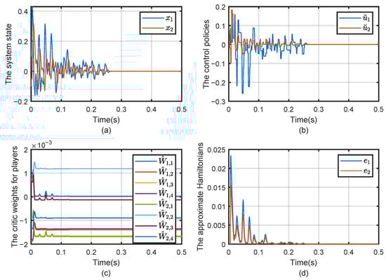
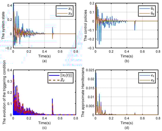
Figure 3. Evolution of (a) the state x, (b) the control strategy ${\breve{u}}_i$, (c) evolution of the critic weigh $\widehat{W_i}$ and (d) the approximate Hamiltonian $e_i$.

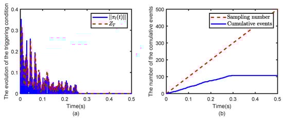
Figure 4. Evolution of (a) the triggering condition and evolution of (b) the cumulative number of triggers.

The state trajectories of the grid-connected VSIs are illustrated in Figure 3a. As observed, the state vectors $x_i={\left[P-P_{\mathrm{ref}},Q-Q_{\mathrm{ref}}\right]}^T$ rapidly converge to zero, demonstrating that both active and reactive power successfully track their respective reference values. This confirms the effectiveness of the proposed adaptive approach in regulating the PQ dynamics, thereby further improving the DC source’s capability to maintain stable synchronization with the interconnected power network, ensuring seamless power exchange and grid stability. Figure 3b illustrates that the control input of each subsystem is updated only when the corresponding event-triggering condition is satisfied, and it eventually converges to zero. This indicates that the proposed strategy achieves aperiodic yet effective control. Moreover, the Hamiltonian functions of all subsystems gradually converge to zero, as shown in Figure 3d, further validating the stability and effectiveness of the proposed method.

The changing trajectories of the critic NN weights are presented in Figure 3c. After the whole system operates for 500 ms, all the weights converged to the following values, where ${\widehat{W}}_1={10}^{-3}·{[0.0202,-1.3977,-1.6539,-1.3519]}^T$, ${\widehat{W}}_2={10}^{-3}·{[-1.6873,1.1855,-0.1299,0.8948]}^T$, respectively.

In Figure 4, once the norm of the event-triggered error $\parallel {\pi }_l\parallel$ exceeds the triggering threshold $Z_T$ and the condition $\parallel {\pi }_l\parallel >Z_T$ is satisfied, an event is triggered for the studied system. Under the designed event-triggered condition, the cumulative number of triggers and the corresponding triggering instants are illustrated in Figure 4. Unlike the time-triggered scheme, which requires 500 samples for the system, the event-triggered scheme significantly reduces the sampling burden, requiring only 107 samples for the system. It can be observed that when the system state enters a small neighborhood around the origin, i.e., $\parallel x\parallel \le \varrho$, the cumulative number of triggers remains unchanged due to the triggering termination condition $\varrho ={10}^{-5}$. This condition effectively reduces unnecessary computations by preventing further triggers once the state stabilizes, thus significantly conserving computational resources.

To further evaluate the grid-current quality of the proposed ADP-based control method, a switching-level single-phase VSI model was reconstructed and driven by the learned control signal. The control signal $u\left(t\right)$ was mapped to a sinusoidal PWM modulation depth and applied to an L–R grid filter to obtain the actual inductor/grid current waveform. Figure 5 shows the full-horizon inductor current and the extracted steady-state current used for harmonic analysis. The corresponding THD is found to be 2.79% which satisfies the typical <5% grid-code requirement.

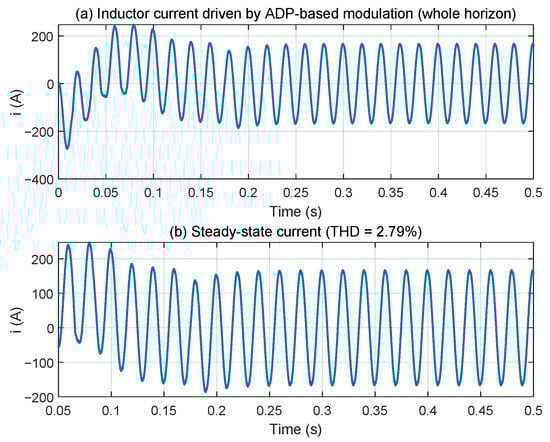
Figure 5. Grid current under the proposed control method.

Case 2. 

To evaluate the robustness of the proposed adaptive control strategy, an additional simulation is conducted in which the initial values of the system’s active and reactive powers are changed after the system has already stabilized and reached its reference power values. This experiment simulates the scenario where, after the system is running stably, changes in initial power values occur at $t=0.5\mathrm{s}$ due to load variations or external disturbances, testing how the system recovers stability and continues to track the target power. The resulting simulation results are presented in Figure 6.

Figure 6. Evolution of (a) the state x, (b) the control strategy ${\breve{u}}_i$, evolution of (c) the triggering condition and (d) the approximate Hamiltonian $e_i$.

As shown in Figure 6, the system state, input control signals, and the approximate Hamiltonian change rapidly at $t=500 \mathrm{ms}$. These signals then converge to zero, indicating that the power tracking and grid synchronization objectives are successfully achieved.

Case 3. 

In this case, a further simulation is conducted to evaluate the performance of the proposed adaptive control strategy when key electrical parameters are varied. The filter inductance $L=4\mathrm{mH}$, filter resistance $R=0.7\Omega$, and nominal grid frequency $f=60\mathrm{Hz}$. The resulting simulation results are presented in Figure 7 and Figure 8.

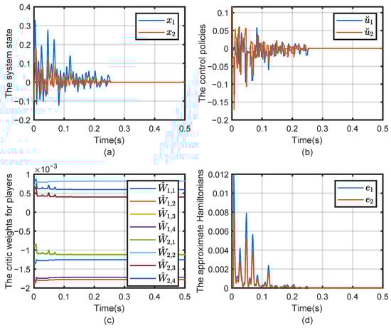
Figure 7. Evolution of (a) the state x, (b) the control strategy ${\breve{u}}_i$, (c) evolution of the critic weigh $\widehat{W_i}$ and (d) the approximate Hamiltonian $e_i$.

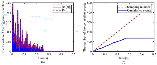
Figure 8. Evolution of (a) the triggering condition and evolution of (b) the cumulative number of triggers.

The state trajectories shown in Figure 7a rapidly converge to zero, indicating that the active and reactive powers successfully track their respective reference values under the new parameter configuration. As in the first experiment, the control inputs are updated only when the event-triggering condition is satisfied, as illustrated in Figure 7b, and the Hamiltonian functions converge to zero, as shown in Figure 7d, further validating the stability and effectiveness of the method. The changing trajectories of the critic NN weights are presented in Figure 7c. After the whole system operates for 500 ms, all the weights converged to the following values, where ${\widehat{W}}_1={10}^{-3}·{[0.5959,-1.7743,-1.1133,-1.7174]}^T$, ${\widehat{W}}_2={10}^{-3}·{[-1.1124,0.8170,0.4003,1.2526]}^T$, respectively.

In Figure 8, the event-triggered condition again demonstrates significant savings in computational resources, with the number of triggers reduced compared to the time-triggered scheme. The system continues to maintain efficient operation with only 136 samples required, confirming that the adaptive control strategy remains effective and computationally efficient even under modified system parameters.

The simulation validates that, despite the changes in electrical parameters, the system continues to demonstrate stable power tracking and grid synchronization. This further confirms the robustness and adaptability of the proposed adaptive control approach, ensuring that the system can maintain performance under varying operational conditions.

Reconfirm the relevant parameters to prove that the proposed algorithm meets the grid connection standards. The control signal $u\left(t\right)$ was mapped to a sinusoidal PWM modulation depth and applied to an L–R grid filter to obtain the actual inductor/grid current waveform. Figure 9 shows the full-horizon inductor current and the extracted steady-state current used for harmonic analysis. The corresponding THD is found to be 2.35% which satisfies the typical <5% grid-code requirement.

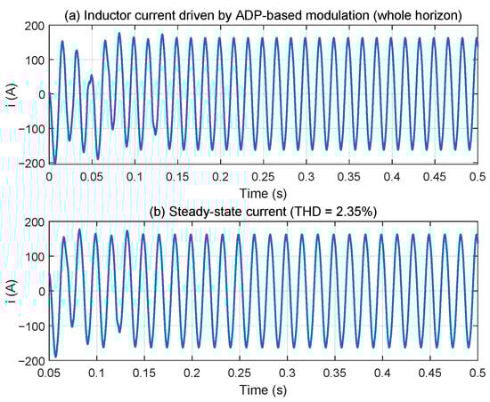
Figure 9. Grid current under the proposed control method.

Case 4. 

To further evaluate the advantages of the proposed ADP-based event-triggered control strategy, a comparative study with a conventional proportional–integral (PI) controller is carried out. In this case, the ADP controller is trained during the interval 0–0.3 s, where the critic neural networks learn the optimal value function under persistently excited system dynamics. After the training stage, the obtained convergent optimal control policy is fixed and directly applied to the VSI power regulation system for the remaining time.

For comparison, a baseline PI controller is designed using proportional gains $K_p=\mathrm{diag}(0.08,0.08)$ and integral gains $K_i=\mathrm{diag}(15,15)$, ensuring a reasonable transient behavior in nominal conditions. Unlike the ADP controller, the PI scheme updates its control action at every sampling instant and does not incorporate any learning or optimization mechanism. To test the robustness of the two controllers, three disturbances of different magnitudes and directions are injected into the power error states at 0.35 s, 0.40 s, and 0.45 s, respectively. These disturbances emulate sudden variations in the operating conditions of the inverter.

The simulation results in Figure 10 demonstrate that although both controllers achieve convergence under normal operating conditions, the ADP-ET controller exhibits noticeably faster decay, smaller fluctuation amplitudes, and significantly quicker recovery after disturbances, highlighting its superior transient performance and robustness compared to the conventional PI strategy.

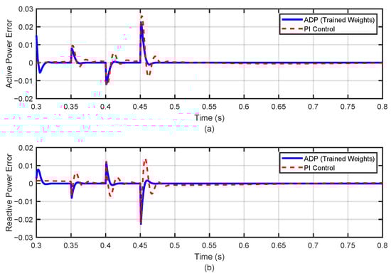
Figure 10. Comparison of ADP and PI control under multiple disturbances: (a) active power error; (b) reactive power error.

5. Conclusions

This paper proposed an optimal control scheme for three-phase grid-connected VSIs. By applying VM-DPC, the nonlinear dynamics were simplified into an LTI form, enabling a tractable design framework. The power regulation problem was modeled as a nonzero-sum game and solved using an ADP approach with a critic NN. An event-triggered mechanism was further incorporated to reduce redundant computation while preserving stability. The overall scheme combines model simplification, online learning, and event-driven updating in a unified framework, providing improved dynamic performance, reduced computational load, and strong adaptability to model uncertainties. Simulation results confirmed accurate power tracking, enhanced dynamics, and efficient implementation.

Future work will focus on implementing the proposed control scheme on a Hardware-in-the-Loop(HIL) or laboratory hardware platform, extending the method to multi-phase and multi-converter systems, and incorporating grid disturbances and stability constraints into the learning framework.

References

- Chang, G.W.; Nguyen, K.T. A New Adaptive Inertia-Based Virtual Synchronous Generator with Even Inverter Output Power Sharing in Islanded Microgrid. IEEE Trans. Ind. Electron. 2024, 71, 10693–10703. [Google Scholar] [CrossRef]
- Chandan, B.; Kumar Pal, P.; Chandra Jana, K.; Siwakoti, Y.P. Performance Evaluation of a New Transformerless Grid-Connected Six-Level Inverter With Integrated Voltage Boosting. IEEE J. Emerg. Sel. Top. Power Electron. 2024, 12, 4361–4376. [Google Scholar] [CrossRef]
- Muraleedharan, N.; Mishra, M.K. Voltage Ride-Through Strategy for Grid-Connected Dual Voltage Source Inverter Under Unsymmetrical Fault Conditions. IEEE Trans. Power Electron. 2025, 40, 17438–17450. [Google Scholar] [CrossRef]
- Ebrahimi, J.; Eren, S. A Multi-Source DC/AC Converter for Integrated Hybrid Energy Storage Systems. IEEE Trans. Energy Convers. 2022, 37, 2298–2309. [Google Scholar] [CrossRef]
- Schweizer, M.; Almér, S.; Pettersson, S.; Merkert, A.; Bergemann, V.; Harnefors, L. Grid-Forming Vector Current Control. IEEE Trans. Power Electron. 2022, 37, 13091–13106. [Google Scholar] [CrossRef]
- Lunardi, A.; Conde, E.; Rocha, N.; Sguarezi Filho, A. Direct power control for DFIG systems under distorted voltage using predictive repetitive control. Int. J. Electr. Power Energy Syst. 2025, 165, 110465. [Google Scholar] [CrossRef]
- Rath, A.; Pratap Behera, B.; Kumar Sethi, B. Improved Shunt Active Filter for Non-Ideal Grid Using Model Predictive and Sliding Mode Control. IEEE Trans. Consum. Electron. 2024, 70, 6600–6608. [Google Scholar] [CrossRef]
- Shen, H.; Xu, J.; Zhang, Q.; Park, J.H.; Peng, C. An Optimal Control Scheme for Grid-Connected Voltage Source Inverter via Grid Voltage Modulated-Direct Power Control. IEEE Trans. Autom. Sci. Eng. 2025, 22, 7216–7225. [Google Scholar] [CrossRef]
- Gui, Y.; Blaabjerg, F.; Wang, X.; Bendtsen, J.D.; Yang, D.; Stoustrup, J. Improved DC-Link Voltage Regulation Strategy for Grid-Connected Converters. IEEE Trans. Ind. Electron. 2021, 68, 4977–4987. [Google Scholar] [CrossRef]
- Gong, Z.; Liu, C.; Shang, L.; Lai, Q.; Terriche, Y. Power Decoupling Strategy for Voltage Modulated Direct Power Control of Voltage Source Inverters Connected to Weak Grids. IEEE Trans. Sustain. Energy 2023, 14, 152–167. [Google Scholar] [CrossRef]
- Aragon, C.A.; Guzman, R.; de Vicuña, L.G.; Miret, J.; Castilla, M. Constrained Predictive Control Based on a Large-Signal Model for a Three-Phase Inverter Connected to a Microgrid. IEEE Trans. Ind. Electron. 2022, 69, 6497–6507. [Google Scholar] [CrossRef]
- Zheng, C.; Dragičević, T.; Majmunović, B.; Blaabjerg, F. Constrained Modulated Model-Predictive Control of an LC-Filtered Voltage-Source Converter. IEEE Trans. Power Electron. 2020, 35, 1967–1977. [Google Scholar] [CrossRef]
- Wang, Z.; Yu, Y.; Gao, W.; Davari, M.; Deng, C. Adaptive, Optimal, Virtual Synchronous Generator Control of Three-Phase Grid-Connected Inverters Under Different Grid Conditions—An Adaptive Dynamic Programming Approach. IEEE Trans. Ind. Inform. 2022, 18, 7388–7399. [Google Scholar] [CrossRef]
- Davari, M.; Gao, W.; Aghazadeh, A.; Blaabjerg, F.; Lewis, F.L. An Optimal Synchronization Control Method of PLL Utilizing Adaptive Dynamic Programming to Synchronize Inverter-Based Resources With Unbalanced, Low-Inertia, and Very Weak Grids. IEEE Trans. Autom. Sci. Eng. 2025, 22, 24–42. [Google Scholar] [CrossRef]
- Liu, D.; Baldi, S.; Yu, W.; Chen, G. On Distributed Implementation of Switch-Based Adaptive Dynamic Programming. IEEE Trans. Cybern. 2022, 52, 7218–7224. [Google Scholar] [CrossRef] [PubMed]
- Liu, D.; Yu, W.; Baldi, S.; Cao, J.; Huang, W. A Switching-Based Adaptive Dynamic Programming Method to Optimal Traffic Signaling. IEEE Trans. Syst. Man Cybern. Syst. 2020, 50, 4160–4170. [Google Scholar] [CrossRef]
- Mi, Z.; Su, H.; Sun, Q.; Cai, Y.; Ming, Z. Dynamic event-triggered-based adaptive frequency control of microgrids under cyber-attacks via adaptive dynamic programming. IET Renew. Power Gener. 2025, 19, e13187. [Google Scholar] [CrossRef]
- Zhang, Y.; Sun, Q.; Zhou, J.; Guerrero, J.M.; Wang, R.; Lashab, A. Optimal Frequency Control for Virtual Synchronous Generator Based AC Microgrids via Adaptive Dynamic Programming. IEEE Trans. Smart Grid 2023, 14, 4–16. [Google Scholar] [CrossRef]
- Zhang, K.; Zhang, Z.X.; Xie, X.P.; Rubio, J.d.J. An Unknown Multiplayer Nonzero-Sum Game: Prescribed-Time Dynamic Event-Triggered Control via Adaptive Dynamic Programming. IEEE Trans. Autom. Sci. Eng. 2025, 22, 8317–8328. [Google Scholar] [CrossRef]
- Su, H.; Zhang, H.; Liang, X.; Liu, C. Decentralized Event-Triggered Online Adaptive Control of Unknown Large-Scale Systems Over Wireless Communication Networks. IEEE Trans. Neural Netw. Learn. Syst. 2020, 31, 4907–4919. [Google Scholar] [CrossRef]
- Xue, S.; Liu, Z.; Wang, L.; Zhang, W.; Ren, K.; Yang, X. Adaptive dynamic programming based event-triggered multi-H∞ control. Neurocomputing 2025, 638, 130157. [Google Scholar] [CrossRef]
- Zhang, Y.; Zhao, B.; Liu, D.; Zhang, S. Adaptive Dynamic Programming-Based Event-Triggered Robust Control for Multiplayer Nonzero-Sum Games With Unknown Dynamics. IEEE Trans. Cybern. 2023, 53, 5151–5164. [Google Scholar] [CrossRef] [PubMed]
- Wang, Z.; Wei, Q.; Liu, D. Event-triggered adaptive dynamic programming for discrete-time multi-player games. Inf. Sci. 2020, 506, 457–470. [Google Scholar] [CrossRef]
- Su, H.; Zhang, H.; Gao, D.W.; Luo, Y. Adaptive Dynamics Programming for H∞ Control of Continuous-Time Unknown Nonlinear Systems via Generalized Fuzzy Hyperbolic Models. IEEE Trans. Syst. Man Cybern. Syst. 2020, 50, 3996–4008. [Google Scholar] [CrossRef]
- Yang, X.; He, H. Event-Driven H∞-Constrained Control Using Adaptive Critic Learning. IEEE Trans. Cybern. 2021, 51, 4860–4872. [Google Scholar] [CrossRef]
Disclaimer/Publisher’s Note: The statements, opinions and data contained in all publications are solely those of the individual author(s) and contributor(s) and not of MDPI and/or the editor(s). MDPI and/or the editor(s) disclaim responsibility for any injury to people or property resulting from any ideas, methods, instructions or products referred to in the content. |
© 2025 by the authors. Licensee MDPI, Basel, Switzerland. This article is an open access article distributed under the terms and conditions of the Creative Commons Attribution (CC BY) license (https://creativecommons.org/licenses/by/4.0/).