Dynamic Analysis and Design of Cylindrical Roller Bearings with Arc End Surfaces of Rollers

Abstract

The new contact model for arc end surfaces of rollers and flanges is established in a dynamic model for cylindrical roller bearings. The dynamic behaviors between roller arc end surfaces and flanges, i.e., contact pressures, sliding velocities, and PV values (peak contact pressure P × sliding velocity V), are investigated and compared to those between roller corners and flanges. Based on the indicators of contact heights and axial clearances, the selection ranges of layback angles, flange axial clearances, and end radius of rollers are proposed, thereby ensuring the bearing operates normally. The results indicate that arc end surfaces are beneficial in reducing contact pressures, sliding velocities, and PV values acting on flanges, especially under high-speed conditions. With less layback angles of flanges and end radii of rollers, contact positions on rollers are more concentrated and the sliding velocity decreases obviously. However, flange heights need to be increased to prevent contact heights between rollers and flanges within the limited zones. Furthermore, since the end radius of rollers leads to a decrease in the axial clearance of flanges, the actual clearance of flanges under axial direction needs to be widened.

1. Introduction

Cylindrical roller bearings in aircraft are usually used for conditions with high speeds and low radial loads [1]. Due to the low limitation of the loads, the stability of the rollers will decrease. Different from the circumferential rotations of rollers, axial movements of rollers and larger relative sliding velocities may lead to a large impact on flanges, which is the main reason for violent wear between rollers and flanges. Traditional contact between rollers and flanges is treated as roller corners and flanges in most research [1,2,3,4,5]. This leads to large pressures, sliding velocities, and PV values (peak contact pressure P × sliding velocity V) because of the low value of the roller corner radius. If arcs on roller end surfaces are adopted, the pressures, sliding velocities, and PV values may decrease significantly with larger radii on roller end surfaces. However, research in related aspects is relatively scarce.

The dynamic behavior of rolling bearings has been the subject of extensive research. The pioneering work by Gupta [2,3,4,5] established fundamental dynamic models that have served as the basis for subsequent studies. These models have enabled accurate prediction and enhancement of critical performance characteristics, such as roller–raceway dynamic contact behaviors [6,7,8], roller–ring misalignment effects [9,10,11], and cage dynamics [12,13,14,15]. The influence of surface waviness on bearing dynamics has been extensively examined in studies [16,17,18,19,20]. Research findings demonstrated that raceway waviness significantly increased roller–raceway contact stiffness while simultaneously inducing severe impacts between rollers and cage pockets. These effects substantially altered the dynamic behaviors and operational stabilities. The dynamic behaviors of a cylindrical roller bearing with a trilobe outer raceway were investigated [1]. The out-of-roundness of the trilobe outer raceway led to an obvious decrease in both the slip ratio of the cage and the relative sliding velocity between the roller and inner ring. However, with an increase in out-of-roundness, the peak values of contact force and pressure increased significantly.

Research on bearing slipping has been conducted based on dynamic bearing analysis methods [21,22,23,24,25]. The traction force acting on rolling elements was identified as a critical factor influencing slipping [21]. The dynamic response of bearings was examined under conditions where both inner and outer rings rotate simultaneously [22]. Significant slipping was observed when the rings rotated in the same direction, accompanied by increased cage slipping and higher relative sliding velocities between rollers and rings. Mitigation strategies for slipping include reducing the number of rollers [23,24] and lowering lubricant density [25], which were found to effectively minimize slipping in bearing systems.

Research on roller–flange contact was discussed in several studies [26,27,28,29]. The interaction tolerance of rollers and flanges was investigated [26,27]. The parametric study demonstrated that optimizing the flange angle and roller–corner radius within tolerance effectively mitigates contact ellipse truncation. Furthermore, variations in roller length were found to significantly alter the axial load distribution characteristics of the bearing system. The failure analysis of the flange was analyzed [28,29]. The results showed that under conditions of high inner-ring misalignment with radial loading, the bearing life initially decreases with increasing flange angle. Excessive axial force caused a great deformation increase in the inner-ring raceway, which induced high local contact stress between one side of the raceway, as well as the corresponding ends of the rollers, resulting in bearing failure.

Although the references [26,27,28,29] were discussed in the contact behavior of the roller corner and the flange, the interference between arc end surfaces of rollers and flanges was not established. Additionally, the dynamic behaviors were not investigated by using the dynamic model of cylindrical roller bearings with consideration of rollers owning arc end surfaces. Therefore, the focus of this paper is on building a new model for the interference between the arc end surfaces of the rollers and flanges. Then the contact pressures, sliding velocities, as well as PV values, are compared to the same conditions with the contact between roller corners and flanges by using the dynamic model of cylindrical roller bearings. Through comparison, it was determined that the contact pressures, sliding velocities, and PV values were obviously reduced by the arc end surfaces of rollers instead of corners.

In this work, an improved contact model between arc end surfaces of rollers and flanges is established. The comparison between different contacts is investigated, especially in high-speed conditions. Then, the ranges of layback angles, radii of roller end surfaces, flange heights, and axial clearance on the raceways are put forward. The paper structure can be summarized as follows: a dynamic model for cylindrical roller bearings is established in Section 2. The results for dynamic behaviors and influence factors are discussed in Section 3. The model and method proposed in this study are validated in Section 4. Section 5 provides a summary of the conclusions.

2. Modeling

The model is based on the existing references, which are in our previous research of Section 2 [1,22], especially for the contact between rollers and ring raceways, rollers and pockets, and the cage and the landing ring. The contact model between roller corners and flanges is discussed in previous works and revisited in Section 2.1.

On the contrary, the new model between roller end surfaces and flanges is established with consideration of arcs on roller end surfaces. The cylindrical roller bearing, which is composed of an inner ring, an outer ring, rollers, and a cage, is illustrated in Figure 1. Table 1 lists the property parameters of the bearing. The initial conditions are the rotating speed and the radial load.

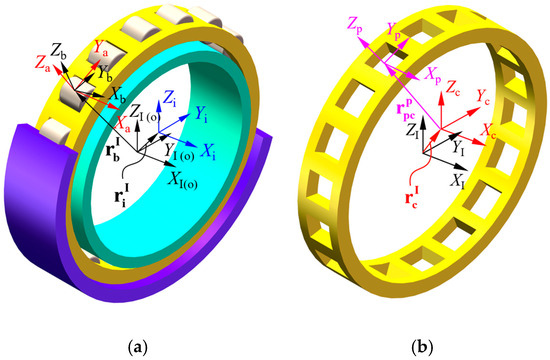
Figure 1. Coordinates of the cylindrical roller bearing on (a) the whole bearing and (b) the cage.

Table 1. Parameters of the cylindrical roller bearing.

Parameters	Symbol	Value
Outer radius (mm)	$R_{o,u}$	40
Inner radius (mm)	$R_{i,d}$	20
Roller radius (mm)	$R_b$	3.75
Roller length (mm)	$L_{b1}$	0.2
Roller central length (mm)	$L_{b2}$	2
End radius of roller (mm)	$R_{\mathrm{end}}$	60–120
Roller corner (mm)	$R_{\mathrm{cor}}$	0.2
Flange height (mm)	$H_{\mathrm{rf}}$	2
Layback angle of flange (°)	${\mathsf{\theta }}_{\mathrm{rrf}}^r$	1.6
Elastic modulus of roller and rings (GPa)	$E_b, E_i, E_o$	203
Elastic modulus of cage (GPa)	$E_c$	205
Poisson’s ratio of roller and rings	${\mathsf{\nu }}_b, {\mathsf{\nu }}_i, {\mathsf{\nu }}_o$	0.28
Poisson’s ratio of cage	${\mathsf{\nu }}_c$	0.29

The inputs are the positions and velocities (including translational and angular velocities) of components under the azimuth and internal coordinate system, i.e., roller positions ($x_b^a$, $r_b^a$, ${\mathsf{\theta }}_b^a$), cage position ($x_c^I$, $y_c^I$, $z_c^I$), inner-ring position ($x_i^I$, $y_i^I$, $z_i^I$), roller velocity ($\mathrm{d}{x}_b^a/\mathrm{d}t$, $\mathrm{d}{r}_b^a/\mathrm{d}t$, $\mathrm{d}{\mathsf{\theta }}_b^a/\mathrm{d}t$), cage velocity ($\mathrm{d}{x}_c^I/\mathrm{d}t$, $\mathrm{d}{y}_c^I/\mathrm{d}t$, $\mathrm{d}{z}_c^I/\mathrm{d}t$), inner-ring velocity ($\mathrm{d}{x}_i^I/\mathrm{d}t$, $\mathrm{d}{y}_i^I/\mathrm{d}t$, $\mathrm{d}{z}_i^I/\mathrm{d}t$), roller angular velocities (${\mathsf{\omega }}_{b,x}^b$, ${\mathsf{\omega }}_{b,\mathrm{y}}^b$, ${\mathsf{\omega }}_{b,z}^b$), cage angular velocity (${\mathsf{\omega }}_{c,x}^c$, ${\mathsf{\omega }}_{c,y}^c$, ${\mathsf{\omega }}_{c,z}^c$), and angular velocity of the inner ring (${\mathsf{\omega }}_{i,x}^i$, ${\mathsf{\omega }}_{i,y}^i$, ${\mathsf{\omega }}_{i,z}^i$), while the outputs are the forces and moments acting on components from the inputs and the positions of components on the next timestep. Notably, all the inputs at the first step are obtained by the quasi-static model in ref. [30] (pp. 64–75). Thereby, the positions and velocities of arbitrary components are generated as the initial values for the dynamic model. The initial rotating speed $n_i$ is set to 20,000 r/min on the inner ring along the $X_i$ axis. The radial load $F_z^I$ is 1000 N and acts on the inner ring along the $Z_{\mathrm{i}}$ axis. The outer ring is fixed.

2.1. Bearing Coordinates

The $O_{\mathrm{I}}-X_{\mathrm{I}}-Y_{\mathrm{I}}-Z_{\mathrm{I}}$, $O_{\mathrm{a}}-X_{\mathrm{a}}-Y_{\mathrm{a}}-Z_{\mathrm{a}}$, $O_{\mathrm{b}}-X_{\mathrm{b}}-Y_{\mathrm{b}}-Z_{\mathrm{b}}$, $O_{\mathrm{o}}-X_{\mathrm{o}}-Y_{\mathrm{o}}-Z_{\mathrm{o}}$, $O_{\mathrm{i}}-X_{\mathrm{i}}-Y_{\mathrm{i}}-Z_{\mathrm{i}}$, $O_{\mathrm{c}}-X_{\mathrm{c}}-Y_{\mathrm{c}}-Z_{\mathrm{c}}$, and $O_{\mathrm{p}}-X_{\mathrm{p}}-Y_{\mathrm{p}}-Z_{\mathrm{p}}$ are the inertial, roller-azimuth, roller-fixed, outer-ring-fixed, inner-ring-fixed, cage-fixed, and cage-pocket-fixed coordinate systems in Figure 1, respectively (more details can be found in Section 2.1 of ref. [1,22]). The transformation from the arbitrary coordinate system $O_{\mathrm{m}}-X_{\mathrm{m}}-Y_{\mathrm{m}}-Z_{\mathrm{m}}$ to the coordinate system $O_{\mathrm{n}}-X_{\mathrm{n}}-Y_{\mathrm{n}}-Z_{\mathrm{n}}$ can be obtained by sequentially rotating around the corresponding coordinate axis, and the angle of rotation is called the Cardan angle (${\mathsf{\eta }}_{\mathrm{m}}^{\mathrm{n}}$, ${\mathsf{\xi }}_{\mathrm{m}}^{\mathrm{n}}$, ${\mathsf{\lambda }}_{\mathrm{m}}^{\mathrm{n}}$). Thereby, the transformation matrix from the arbitrary coordinate system $O_{\mathrm{m}}-X_{\mathrm{m}}-Y_{\mathrm{m}}-Z_{\mathrm{m}}$ to the coordinate system $O_{\mathrm{n}}-X_{\mathrm{n}}-Y_{\mathrm{n}}-Z_{\mathrm{n}}$ can be expressed as

$$\left[T\left({\eta }_{\mathrm{m}}^{\mathrm{n}},{\xi }_{\mathrm{m}}^{\mathrm{n}},{\lambda }_{\mathrm{m}}^{\mathrm{n}}\right)\right]=\left[\begin{array}{ccc}\cos {\xi }_{\mathrm{m}}^{\mathrm{n}}\cos {\lambda }_{\mathrm{m}}^{\mathrm{n}}& \cos {\eta }_{\mathrm{m}}^{\mathrm{n}}\sin {\lambda }_{\mathrm{m}}^{\mathrm{n}}+\sin {\eta }_{\mathrm{m}}^{\mathrm{n}}\sin {\xi }_{\mathrm{m}}^{\mathrm{n}}\cos {\lambda }_{\mathrm{m}}^{\mathrm{n}}& \sin {\eta }_{\mathrm{m}}^{\mathrm{n}}\sin {\lambda }_{\mathrm{m}}^{\mathrm{n}}-\cos {\eta }_{\mathrm{m}}^{\mathrm{n}}\sin {\xi }_{\mathrm{m}}^{\mathrm{n}}\cos {\lambda }_{\mathrm{m}}^{\mathrm{n}}\\ -\cos {\xi }_{\mathrm{m}}^{\mathrm{n}}\sin {\lambda }_{\mathrm{m}}^{\mathrm{n}}& \cos {\eta }_{\mathrm{m}}^{\mathrm{n}}\cos {\lambda }_{\mathrm{m}}^{\mathrm{n}}-\sin {\eta }_{\mathrm{m}}^{\mathrm{n}}\sin {\xi }_{\mathrm{m}}^{\mathrm{n}}\sin {\lambda }_{\mathrm{m}}^{\mathrm{n}}& \sin {\eta }_{\mathrm{m}}^{\mathrm{n}}\cos {\lambda }_{\mathrm{m}}^{\mathrm{n}}+\cos {\eta }_{\mathrm{m}}^{\mathrm{n}}\sin {\xi }_{\mathrm{m}}^{\mathrm{n}}\sin {\lambda }_{\mathrm{m}}^{\mathrm{n}}\\ \sin {\xi }_{\mathrm{m}}^{\mathrm{n}}& -\sin {\eta }_{\mathrm{m}}^{\mathrm{n}}\cos {\xi }_{\mathrm{m}}^{\mathrm{n}}& \cos {\eta }_{\mathrm{m}}^{\mathrm{n}}\cos {\xi }_{\mathrm{m}}^{\mathrm{n}}\end{array}\right]$$

(1)

2.2. Dynamic Contact Model Between Rollers and Flanges

2.2.1. Interference Between Roller Corners and Flanges

Figure 2 shows the interference between the roller and the flange, while r = o/i represents the outer or inner ring.

Figure 2. Relationship of the roller corners and flanges on the (a) left side of the outer ring; (b) right side of the outer ring; (c) left side of the inner ring; and (d) right side of the inner ring, which are given by Equations (2), (3) and (5)–(7).

The vector located at the roller center from the ring center under the ring-fixed coordinate system can be expressed as

$$r_{br}^r=T_{Ir}\left(r_b^I-r_r^I\right)$$

(2)

where ${\mathrm{T}}_{\mathrm{Ir}}({\mathsf{\eta }}_{\mathrm{r}}^{\mathrm{I}},{\mathsf{\xi }}_{\mathrm{r}}^{\mathrm{I}},{\mathsf{\lambda }}_{\mathrm{r}}^{\mathrm{I}})$ represents the transformation matrixes from the inertial coordinate system to the ring-fixed coordinate system. ${\mathrm{r}}_{\mathrm{b}}^{\mathrm{I}}$ and ${\mathrm{r}}_{\mathrm{r}}^{\mathrm{I}}$ represent the vectors from the origin of the inertial coordinate system to the roller center and ring center, respectively.

The vector located at the left and right sides of the corner center from the roller center under the flange coordinate system can be expressed as

$$r_{bcb}^{rf}=T_{rarf}{T}_{rra}{T}_{Ir}{T_{Ib}}^{\prime }{r}_{bcb}^b=T_{brf}{\left[\pm L_{\mathrm{bcb}},-R_{\mathrm{ce}}\sin {\phi }_{\mathrm{brf}}^{\mathrm{b}},R_{\mathrm{ce}}\cos {\phi }_{\mathrm{brf}}^{\mathrm{b}}\right]}^{\mathrm{T}}$$

(3)

where ${\mathbf{T}}_{\mathbf{raf}}=\mathbf{T}(0,{\mathsf{\theta }}_{\mathrm{rf}}^{\mathrm{r}},{\mathsf{\theta }}_{\mathrm{rrf}}^{\mathrm{r}})$ represents the transformation matrix between the ring-azimuth coordinate system to the flange coordinate system. ${\mathsf{\theta }}_{\mathrm{rf}}^{\mathrm{r}}$ equals 0 for the left side of the ring and equals $\pi$ for the right side of the ring. ${\mathsf{\theta }}_{\mathrm{rrf}}^{\mathrm{r}}$ is the layback angle of each flange on the ring. ${\mathbf{T}}_{\mathbf{raf}}=\mathrm{T}\left({\mathsf{\theta }}_{\mathrm{br}}^{\mathrm{r}},0,0\right)$ is the transformation matrix from the ring-fixed coordinate system to the ring-azimuth coordinate system, and the ring-azimuth is written as ${\mathsf{\theta }}_{\mathrm{br}}^r={\tan }^{-1}(-r_{br,\mathrm{y}}^r/r_{br,\mathrm{z}}^{\mathrm{r}})$. $L_{\mathrm{bcb}}$ represents the distance between the corner center to the roller center, and $\pm$ represents the left and right sides of the ring. $R_{\mathrm{ce}}$ is the radius of the corner center relative to the roller $X_b$ axis. ${\phi }_{\mathrm{brf}}^{\mathrm{b}}$ is the contact angle between the roller and the flange, and can be obtained by

$$\left\{\begin{array}{l}{T}_{\mathrm{rarf},11}\left[-T_{\mathrm{br},12}{R}_{\mathrm{bcb}}\cos {\phi }_{\mathrm{brf}}^{\mathrm{b}}-T_{\mathrm{br},13}{R}_{\mathrm{bcb}}\sin {\phi }_{\mathrm{brf}}^{\mathrm{b}}\right]+\\ {\displaystyle \frac{T_{\mathrm{rarf},13}}{r_{\mathrm{bcr},\mathrm{z}}^{\mathrm{ra}}}}\left[{\displaystyle \sum _{l=2}^3\begin{array}{l}\left(r_{\mathrm{br},l}^{\mathrm{r}}\pm T_{\mathrm{br},l1}{L}_{\mathrm{bcb}}-T_{\mathrm{br},l2}{R}_{\mathrm{bcb}}\sin {\phi }_{\mathrm{brf}}^{\mathrm{b}}+T_{\mathrm{br},l3}{R}_{\mathrm{bcb}}\cos {\phi }_{\mathrm{brf}}^{\mathrm{b}}\right)\times \\ \left(-T_{\mathrm{br},l2}{R}_{\mathrm{bcb}}\cos {\phi }_{\mathrm{brf}}^{\mathrm{b}}-T_{\mathrm{br},l3}{R}_{\mathrm{bcb}}\sin {\phi }_{\mathrm{brf}}^{\mathrm{b}}\right)\end{array}}\right]\end{array}\right\}=0$$

(4)

where ${\mathbf{T}}_{\mathbf{br}} \mathbf{=} {\mathbf{T}}_{\mathbf{Ir}}{{\mathbf{T}}_{\mathbf{Ib}}}^{\prime }$ represents the transformation matrix from the roller-fixed coordinate system to the ring-fixed coordinate system. ${\mathbf{T}}_{\mathbf{Ib}}({\mathsf{\eta }}_{\mathrm{b}}^I,{\mathsf{\xi }}_{\mathrm{b}}^I,{\mathsf{\lambda }}_{\mathrm{b}}^I)$ represents the transformation matrixes from the inertial coordinate system to the roller-fixed coordinate system.

The vector located at the roller corner center from the ring center under the ring-fixed coordinate system can be expressed as

$$r_{bcr}^r={T_{rra}}^{\prime }{T_{rarf}}^{\prime }{r}_{bcb}^{rf}+r_{br}^r$$

(5)

The vector located at the roller corner center to the ring center under the ring-azimuth coordinate system can be expressed as

$$r_{bcr}^{ra}={\left[r_{\mathrm{bcr},\mathrm{x}}^{\mathrm{r}},0,\sqrt{{\left(r_{\mathrm{bcr},\mathrm{y}}^{\mathrm{r}}\right)}^2+{\left(r_{\mathrm{bcr},\mathrm{z}}^{\mathrm{r}}\right)}^2}\right]}^{\mathrm{T}}$$

(6)

The vector located at the origin of the flange coordinate system from the roller corner center under the flange coordinate system can be expressed as

$$r_{rfbc}^{rf}=T_{rarf}\left({\left[\pm 0.5W_{\mathrm{r}},0,R_{\mathrm{rm}}\left({\phi }_{\mathrm{r}}^{\mathrm{r}}\right)\right]}^{\mathrm{T}}-r_{bcr}^{ra}\right)$$

(7)

where $\pm$ represents the right and left side of the ring. $R_{\mathrm{rm}}$ is the radius of the raceway. ${\phi }_{\mathrm{r}}^{\mathrm{r}}$ is the azimuth angle of the ring under the ring-fixed coordinate system. $W_{\mathrm{r}}$ is defined as the raceway width that equals the roller length and the axial clearance, and can be expressed as

$$W_{\mathrm{r}}=L_{b1}+{\Delta }_{\mathrm{bf}}$$

(8)

where $L_{\mathrm{b}1}$ is the length of the roller. ${\mathsf{\Delta }}_{\mathrm{bf}}$ is the axial clearance between the roller and the flange.

The contact vector between the roller corners and flanges is shown in Figure 3.

Figure 3. Contact vectors between the roller corners and flanges, which are given by Equations (9) and (10).

The vector located at the local contact point between the roller and the flange from the ring center under the flange coordinate system can be expressed as

$$r_{rfsr}^{rf}=r_{rfsb}^{rf}+T_{rarf}{T}_{rra}{r}_{br}^r$$

(9)

where ${\mathbf{r}}_{\mathbf{rfsb}}^{\mathbf{rf}}$ represents the vector located at the local contact point between the roller and the flange from the roller center under the flange coordinate system

$$r_{rfsb}^{rf}=r_{bcb}^{rf}+{\left[R_{\mathrm{cor}},0,0\right]}^{\mathrm{T}}$$

(10)

where $R_{\mathrm{cor}}$ represents the radius of the roller.

The interference between the roller and the flange ${\delta }_{\mathrm{brf}}$ can be expressed as

$${\delta }_{\mathrm{brf}}=r_{\mathrm{rfbc},x}^{\mathrm{rf}}-R_{\mathrm{cor}}$$

(11)

The sliding velocity between the roller corner and the flange under the flange coordinate system ${\mathbf{u}}_{\mathbf{brf}}^{\mathbf{rf}}$ can be expressed as

$$u_{brf}^{rf}=T_{brf}{T}_{Ib}{v}_b^I+\left(T_{brf}{\omega }_b^b\right)\times r_{rfsb}^{rf}-T_{rarf}{T}_{rra}{T}_{Ir}{v}_r^I-\left(T_{rarf}{T}_{rra}{\omega }_r^r\right)\times r_{rfsr}^{rf}$$

(12)

where ${\mathbf{v}}_{\mathbf{b}}^{\mathbf{I}}$ and ${\mathbf{v}}_{\mathbf{r}}^{\mathbf{I}}$ represent the translational velocity of the roller and the ring under the inertial coordinate system, respectively. ${\mathsf{\omega }}_{\mathbf{b}}^{\mathbf{b}}$ represents the angular velocity of the roller under the roller-fixed coordinate system. ${\mathsf{\omega }}_{\mathbf{r}}^{\mathbf{r}}$ represents the translational velocity of the ring under the ring-fixed coordinate system.

The contact force between the roller corner and the flange by the traditional Hertz method $Q_{\mathrm{brf}}$ can be expressed as

$$Q_{\mathrm{brf}}=\left\{\begin{array}{l}{K}_{\mathrm{brf}}{\left|{\delta }_{\mathrm{brf}}\right|}^{1.5},r_{\mathrm{rfbc},\mathrm{x}}^{\mathrm{rf}}-R_{\mathrm{cor}}<0\\ 0,r_{\mathrm{rfbc},\mathrm{x}}^{\mathrm{rf}}-R_{\mathrm{cor}}\ge 0\end{array}\right.$$

(13)

where $K_{\mathrm{brf}}$ is the Hertz contact stiffness of the roller corner and the flange [30] and can be expressed as

$$K_{\mathrm{brf}}=\pi E_{\mathrm{brf}}\left[1.0339{\left(r_{\mathrm{x}}/r_{\mathrm{y}}\right)}^{0.636}\right]{\left\{r_{\mathrm{p}}\left[1.0003+0.5968\left(r_{\mathrm{y}}/r_{\mathrm{x}}\right)\right]/\left\{4.5{\left[1.5277+0.6023\ln \left(r_{\mathrm{x}}/r_{\mathrm{y}}\right)\right]}^3\right\}\right\}}^{0.5}$$

(14)

where $r_{\mathrm{x}}$, $r_{\mathrm{y}}$, and $r_{\sigma }$ are, respectively, the curvature radius in the x and y direction, as well as the equivalent radius of curvature, and can be expressed as

$$r_{\mathrm{x}}=1\left(1/R_{\mathrm{cor}}+1/\left(\left(R_{\mathrm{cor}}+R_{\mathrm{ce}}\right)\cos {\theta }_{\mathrm{rrf}}^{\mathrm{r}}\right)\right), r_{\mathrm{y}}=1/\left(1/+\infty +1/R_{\mathrm{rm}}\left({\phi }_{\mathrm{r}}^{\mathrm{r}}\right)\right), r_{\sigma }=1/\left(1/r_{\mathrm{x}}+1/r_{\mathrm{y}}\right)$$

(15)

The PV value between the roller corner and the flange can be expressed as

$$P{V}_{\mathrm{brf}}=p_{\mathrm{brf},\max }\left|u_{brf}^{rf}\right|$$

(16)

where $p_{\mathrm{brf},\max }$ is the peak Hertz contact pressure between the roller corner and the flange.

The resultant force on the roller from the flange under the flange coordinate system can be expressed as

$$F_{brf}^{rf}={\left[\begin{array}{ccc}-Q_{\mathrm{brf}},& {\displaystyle \frac{-{\mu }_{\mathrm{brf}}{Q}_{\mathrm{brf}}{u}_{\mathrm{brf},\mathrm{y}}^{\mathrm{rf}}}{\sqrt{{\left(u_{\mathrm{brf},\mathrm{y}}^{\mathrm{rf}}\right)}^2+{\left(u_{\mathrm{brf},\mathrm{z}}^{\mathrm{rf}}\right)}^2}}},& {\displaystyle \frac{-{\mu }_{\mathrm{brf}}{Q}_{\mathrm{brf}}{u}_{\mathrm{brf},\mathrm{z}}^{\mathrm{rf}}}{\sqrt{{\left(u_{\mathrm{brf},\mathrm{y}}^{\mathrm{rf}}\right)}^2+{\left(u_{\mathrm{brf},\mathrm{z}}^{\mathrm{rf}}\right)}^2}}}\end{array}\right]}^{\mathrm{T}},r_{\mathrm{rfbc},\mathrm{x}}^{\mathrm{rf}}-R_{\mathrm{cor}}<0$$

(17)

where ${\mu }_{\mathrm{brf}}$ is the traction coefficient at the contact position between the roller corner and the flange and equals 0.08 for dry contact.

Then, the resultant forces and moments can be transformed to the corresponding coordinate system and are expressed as

$$\left\{\begin{array}{l}{F}_{brf}^a={\displaystyle \sum _1^2{T}_{Ia}{T_{Ib}}^{\prime }{T_{brf}}^{\prime }{F}_{brf}^{rf}}\hfill \\ F_{rfb}^I={\displaystyle \sum _1^{k_{\mathrm{b}}}{\displaystyle \sum _1^2\left(-{T_{Ir}}^{\prime }{T_{rra}}^{\prime }{T_{rarf}}^{\prime }{F}_{brf}^{rf}\right)}}\hfill \\ M_{brf}^b=T_{Ib}{T_{Ic}}^{\prime }{T_{brf}}^{\prime }\left(r_{rfsb}^{rf}\times F_{brf}^{rf}\right)\hfill \\ M_{rfb}^r={\displaystyle \sum _1^{k_{\mathrm{b}}}{\displaystyle \sum _1^2{T_{rra}}^{\prime }{T_{rarf}}^{\prime }\left(-r_{rfsr}^{rf}\times F_{brf}^{rf}\right)}}\hfill \end{array}\right.$$

(18)

where ${\mathbf{F}}_{\mathbf{bf}}^{\mathbf{a}}$ is the resultant force on the roller from flanges in the roller-azimuth coordinate system. ${\mathbf{F}}_{\mathbf{rfb}}^{\mathbf{I}}$ is the resultant force on the flanges from rollers in the inertial coordinate system. ${\mathbf{M}}_{\mathbf{bf}}^{\mathbf{b}}$ is the resultant moment on the roller from flanges in the roller-fixed coordinate system. ${\mathbf{M}}_{\mathbf{rfb}}^{\mathbf{r}}$ is the resultant moment on the flanges from rollers in the ring-fixed coordinate system.

2.2.2. Interference Between Roller End Surfaces and Flanges

Figure 4 exhibits the interference relationship between the roller end surface and the flange.

Figure 4. Relationship of the roller end surfaces and flanges, which are given by Equations (19)–(21).

The vector located at both sides of the corner center from the roller center under the flange coordinate system can be expressed as

$$r_{beb}^b={\left[L_{\mathrm{beb}},0,0\right]}^{\mathrm{T}}, L_{\mathrm{beb}}=x_{\mathrm{cor}}^{\mathrm{b}}\left({\phi }_{\mathrm{b}}^{\mathrm{b}}\right)\mp \sqrt{{\left(R_{\mathrm{end}}-R_{\mathrm{cor}}\right)}^2-{\left[y_{\mathrm{cor}}^{\mathrm{b}}\left({\phi }_{\mathrm{b}}^{\mathrm{b}}\right)\right]}^2}, {\phi }_{\mathrm{b}}^{\mathrm{b}}=0$$

(19)

where $L_{\mathrm{beb}}$ represents the length of the center of the arc on the roller end surface to the roller center, and $\pm$ represents the left and right side of the ring. $x_{\mathrm{cor}}^{\mathrm{b}}$ and ${\mathrm{z}}_{\mathrm{cor}}^{\mathrm{b}}$ represent the coordinates of the roller corner center in the roller-fixed coordinate system. ${\phi }_{\mathrm{b}}^{\mathrm{b}}$ is the position angle of the roller corner center under the roller-fixed coordinate system. $R_{\mathrm{end}}$ is the radius of the arc end surface.

The vector located at the center of the arc on the roller end surface from the ring center under the ring-fixed coordinate system can be expressed as

$$r_{ber}^r=T_{br}{r}_{beb}^b+r_{br}^r$$

(20)

The vector located at the center of the arc on the roller end surface from the origin of the flange coordinate system under the ring-azimuth coordinate system can be expressed as

$$r_{berf}^{rf}={\left[r_{\mathrm{ber},\mathrm{x}}^{\mathrm{r}}\mp 0.5W_{\mathrm{r}},0,\sqrt{{\left(r_{\mathrm{ber},\mathrm{y}}^{\mathrm{r}}\right)}^2+{\left(r_{\mathrm{ber},\mathrm{z}}^{\mathrm{r}}\right)}^2}-R_{\mathrm{rm}}\left({\phi }_{\mathrm{r}}^{\mathrm{r}}\right)\right]}^{\mathrm{T}}$$

(21)

The contact vector between the roller end surfaces and flanges is shown in Figure 5.

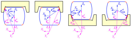
Figure 5. Contact vectors between the roller end surfaces and flanges, which are given by Equations (22) and (23).

The vector located at the local contact point between the roller and the flange from the ring center under the flange coordinate system can be expressed as

$$r_{rfsr}^{rf}=T_{rarf}\left(r_{berf}^{ra}+{\left[\pm 0.5W_{\mathrm{r}},0,R_{\mathrm{rm}}\left({\phi }_{\mathrm{r}}^{\mathrm{r}}\right)\right]}^{\mathrm{T}}\right)+{\left[R_{\mathrm{end}},0,0\right]}^{\mathrm{T}}$$

(22)

Notably, the actual clearance between the roller and the flange needs to be corrected as

$${\Lambda }_{\mathrm{bf}}={\Delta }_{\mathrm{bf}}-\left[\left(R_{\mathrm{end}}-\left|r_{\mathrm{beb},\mathrm{x}}^{\mathrm{b}}\right|\right)-0.5L_{b1}\right]$$

(23)

The vector located at the local contact point between the roller and the flange from the roller center under the flange coordinate system can be expressed as

$$r_{rfsb}^{rf}=r_{rfsr}^{rf}-T_{rarf}{T}_{rra}{T}_{Ir}\left(r_b^I-r_r^I\right)$$

(24)

The interference between the roller and the flange can be expressed as

$${\delta }_{\mathrm{berf}}=-r_{\mathrm{berf},\mathrm{x}}^{\mathrm{rf}}-R_{\mathrm{end}}$$

(25)

The sliding velocity between the roller end surface and the flange under the flange coordinate system can be expressed as

$$u_{berf}^{rf}=T_{brf}{T}_{Ib}{v}_b^I+\left([T_{brf}]{\omega }_b^b\right)\times r_{rfsb}^{rf}-T_{rarf}{T}_{rra}{T}_{Ir}{v}_r^I-\left(T_{rarf}{T}_{rra}{\omega }_r^r\right)\times r_{rfsr}^{rf}$$

(26)

The contact force between the roller end surface and the flange can be expressed as

$$Q_{\mathrm{berf}}=\left\{\begin{array}{l}{K}_{\mathrm{berf}}{\left|{\delta }_{\mathrm{berf}}\right|}^{1.5},r_{\mathrm{berf},\mathrm{x}}^{\mathrm{rf}}+R_{\mathrm{end}}>0\\ 0,r_{\mathrm{berf},\mathrm{x}}^{\mathrm{rf}}+R_{\mathrm{end}}\le 0\end{array}\right.$$

(27)

where $K_{\mathrm{berf}}$ is the Hertz contact stiffness of the roller end surface and the flange, and can be expressed as

$$K_{\mathrm{berf}}=\pi E_{\mathrm{brf}}\left[1.0339{\left(r_{\mathrm{x}}/r_{\mathrm{y}}\right)}^{0.636}\right]{\left\{r_{\mathrm{p}}\left[1.0003+0.5968\left(r_{\mathrm{y}}/r_{\mathrm{x}}\right)\right]/\left\{4.5{\left[1.5277+0.6023\ln \left(r_{\mathrm{x}}/r_{\mathrm{y}}\right)\right]}^3\right\}\right\}}^{0.5}$$

(28)

where $r_{\mathrm{x}}$, $r_{\mathrm{y}}$, and $r_{\sigma }$ are, respectively, the curvature radius in the x and y direction, as well as the equivalent radius of curvature, and can be expressed as

$$r_{\mathrm{x}}=1\left(1/R_{\mathrm{end}}+1/R_{\mathrm{end}}\right), r_{\mathrm{y}}=1/\left(1/+\infty +1/R_{\mathrm{rm}}\left({\phi }_{\mathrm{r}}^{\mathrm{r}}\right)\right), r_{\sigma }=1/\left(1/r_{\mathrm{x}}+1/r_{\mathrm{y}}\right)$$

(29)

The PV value between the roller end surface and the flange can be expressed as

$$P{V}_{\mathrm{berf}}=p_{\mathrm{berf},\max }\left|u_{berf}^{rf}\right|$$

(30)

where p_berf,max is the peak Hertz contact pressure between the roller end surface and the flange.

The resultant force on the roller from the flange under the flange coordinate system can be expressed as

$$F_{brf}^{rf}={\left[\begin{array}{ccc}-Q_{\mathrm{berf}},& {\displaystyle \frac{-{\mu }_{\mathrm{berf}}{Q}_{\mathrm{berf}}{u}_{\mathrm{berf},\mathrm{y}}^{\mathrm{rf}}}{\sqrt{{\left(u_{\mathrm{berf},\mathrm{y}}^{\mathrm{rf}}\right)}^2+{\left(u_{\mathrm{berf},\mathrm{z}}^{\mathrm{rf}}\right)}^2}}},& {\displaystyle \frac{-{\mu }_{\mathrm{berf}}{Q}_{\mathrm{berf}}{u}_{\mathrm{berf},\mathrm{z}}^{\mathrm{rf}}}{\sqrt{{\left(u_{\mathrm{berf},\mathrm{y}}^{\mathrm{rf}}\right)}^2+{\left(u_{\mathrm{berf},\mathrm{z}}^{\mathrm{rf}}\right)}^2}}}\end{array}\right]}^{\mathrm{T}},r_{\mathrm{berf},\mathrm{x}}^{\mathrm{rf}}-R_{\mathrm{end}}>0$$

(31)

where ${\mu }_{\mathrm{berf}}$ is the traction coefficient at the contact position between the roller end surface and the flange and equals 0.08 for dry contact.

Then, the resultant forces and moments can be transformed to the corresponding coordinate system and are expressed as

$$\left\{\begin{array}{l}{F}_{brf}^a={\displaystyle \sum _1^2{T}_{Ia}{T_{Ib}}^{\prime }{T_{brf}}^{\prime }{F}_{brf}^{rf}}\hfill \\ F_{rfb}^I={\displaystyle \sum _1^{k_{\mathrm{b}}}{\displaystyle \sum _1^2\left(-{T_{Ir}}^{\prime }{T_{rra}}^{\prime }{T_{rarf}}^{\prime }{F}_{brf}^{rf}\right)}}\hfill \\ M_{brf}^b=T_{Ib}{T_{Ic}}^{\prime }{T_{brf}}^{\prime }\left(r_{rfsb}^{rf}\times F_{brf}^{rf}\right)\hfill \\ M_{rfb}^r={\displaystyle \sum _1^{k_{\mathrm{b}}}{\displaystyle \sum _1^2{T_{rra}}^{\prime }{T_{rarf}}^{\prime }\left(-r_{rfsr}^{rf}\times F_{brf}^{rf}\right)}}\hfill \end{array}\right.$$

(32)

The dynamic interactions involving rollers and rings, rollers and pockets, and cage and rings, along with the churning forces and moments acting on rollers and the cage, have been investigated in Section 2 of our prior studies [1,22]. Consequently, these aspects will not be discussed within the present work.

2.3. Dynamic Equations

The roller dynamic equations are

$$\left\{\begin{array}{l}{\mathrm{d}}^2\left(x_{\mathrm{b}}^{\mathrm{a}}\right)/\mathrm{d}{t}^2=\left(F_{\mathrm{bo},\mathrm{x}}^{\mathrm{a}}+F_{\mathrm{bi},\mathrm{x}}^{\mathrm{a}}+F_{\mathrm{bf},\mathrm{x}}^{\mathrm{a}}+F_{\mathrm{bc},\mathrm{x}}^{\mathrm{a}}+F_{\mathrm{bd},\mathrm{x}}^{\mathrm{a}}\right)/m_{\mathrm{b}}\\ {\mathrm{d}}^2\left(r_{\mathrm{b}}^{\mathrm{a}}\right)/\mathrm{d}{t}^2=\left(F_{\mathrm{bo},\mathrm{z}}^{\mathrm{a}}+F_{\mathrm{bi},\mathrm{z}}^{\mathrm{a}}+F_{\mathrm{bf},\mathrm{z}}^{\mathrm{a}}+F_{\mathrm{bc},\mathrm{z}}^{\mathrm{a}}+F_{\mathrm{bd},\mathrm{z}}^{\mathrm{a}}+m_{\mathrm{b}}{r}_{\mathrm{b}}^{\mathrm{a}}{\left(\mathrm{d}{\theta }_{\mathrm{b}}^{\mathrm{a}}/\mathrm{d}t\right)}^2+m_{\mathrm{b}}g\cos {\theta }_{\mathrm{b}}^{\mathrm{a}}\right)/m_{\mathrm{b}}\\ {\mathrm{d}}^2\left({\theta }_{\mathrm{b}}^{\mathrm{a}}\right)/\mathrm{d}{t}^2=\left(-F_{\mathrm{bo},\mathrm{y}}^{\mathrm{a}}-F_{\mathrm{bi},\mathrm{y}}^{\mathrm{a}}-F_{\mathrm{bf},\mathrm{y}}^{\mathrm{a}}-F_{\mathrm{bc},\mathrm{y}}^{\mathrm{a}}-F_{\mathrm{bd},\mathrm{y}}^{\mathrm{a}}-2m_{\mathrm{b}}\left(\mathrm{d}{r}_{\mathrm{b}}^{\mathrm{a}}/\mathrm{d}t\right)\left(\mathrm{d}{\theta }_{\mathrm{b}}^{\mathrm{a}}/\mathrm{d}t\right)-m_{\mathrm{b}}g\sin {\theta }_{\mathrm{b}}^{\mathrm{a}}\right)/r_{\mathrm{b}}^{\mathrm{a}}/m_{\mathrm{b}}\\ \mathrm{d}{\omega }_{\mathrm{b},\mathrm{x}}^{\mathrm{b}}/\mathrm{d}t=\left(M_{\mathrm{bo},\mathrm{x}}^{\mathrm{b}}+M_{\mathrm{bi},\mathrm{x}}^{\mathrm{b}}+M_{\mathrm{bf},\mathrm{x}}^{\mathrm{b}}+M_{\mathrm{bc},\mathrm{x}}^{\mathrm{b}}\right)/I_{\mathrm{b},\mathrm{x}}\\ \mathrm{d}{\omega }_{\mathrm{b},\mathrm{y}}^{\mathrm{b}}/\mathrm{d}t=\left(M_{\mathrm{bo},\mathrm{y}}^{\mathrm{b}}+M_{\mathrm{bi},\mathrm{y}}^{\mathrm{b}}+M_{\mathrm{bi},\mathrm{y}}^{\mathrm{b}}+M_{\mathrm{bc},\mathrm{y}}^{\mathrm{b}}\right)/I_{\mathrm{b},\mathrm{y}}\\ \mathrm{d}{\omega }_{\mathrm{b},\mathrm{z}}^{\mathrm{b}}/\mathrm{d}t=\left(M_{\mathrm{bo},\mathrm{z}}^{\mathrm{b}}+M_{\mathrm{bi},\mathrm{z}}^{\mathrm{b}}+M_{\mathrm{bi},\mathrm{z}}^{\mathrm{b}}+M_{\mathrm{bc},\mathrm{z}}^{\mathrm{b}}\right)/I_{\mathrm{b},\mathrm{z}}\end{array}\right.$$

(33)

where $m_{\mathrm{b}}$ represents the mass of rollers. $I_{\mathrm{b}}$ represents the inertia moments of rollers. ${\mathbf{F}}_{\mathbf{bo}}^{\mathbf{a}}, {\mathbf{F}}_{\mathbf{bi}}^{\mathbf{a}}, {\mathbf{F}}_{\mathbf{bf}}^{\mathbf{a}}, {\mathbf{F}}_{\mathbf{bc}}^{\mathbf{a}},$ and ${\mathbf{F}}_{\mathbf{bd}}^{\mathbf{a}}$ are resultant forces acting on the roller from the outer ring, inner ring, flanges, cage pocket, and oil churning, respectively. ${\mathbf{M}}_{\mathbf{bo}}^{\mathbf{b}}, {\mathbf{M}}_{\mathbf{bi}}^{\mathbf{b}}, {\mathbf{M}}_{\mathrm{bf}}^{\mathbf{b}}, \mathrm{and} {\mathbf{M}}_{\mathbf{bc}}^{\mathbf{b}}$ are resultant moments acting on the roller from the outer ring, inner ring, flanges, and cage pocket, respectively. The coordinate system is defined by three axes, labeled x, y, and z, as denoted by the subscripts.

The cage dynamic equations are

$$\left\{\begin{array}{l}{\mathrm{d}}^2\left(y_{\mathrm{c}}^{\mathrm{I}}\right)/\mathrm{d}{t}^2=\left(F_{\mathrm{cb},\mathrm{y}}^{\mathrm{I}}+F_{\mathrm{co},\mathrm{y}}^{\mathrm{I}}\right)/m_{\mathrm{c}}\\ {\mathrm{d}}^2\left(z_{\mathrm{c}}^{\mathrm{I}}\right)/\mathrm{d}{t}^2=\left(F_{\mathrm{cb},\mathrm{z}}^{\mathrm{I}}+F_{\mathrm{co},\mathrm{z}}^{\mathrm{I}}+m_{\mathrm{c}}g\right)/m_{\mathrm{c}}\\ \mathrm{d}{\omega }_{\mathrm{c},\mathrm{x}}^{\mathrm{c}}/\mathrm{d}t=\left(M_{\mathrm{cb},\mathrm{x}}^{\mathrm{c}}+M_{\mathrm{co},\mathrm{x}}^{\mathrm{c}}+M_{\mathrm{cd},\mathrm{x}}^{\mathrm{c}}\right)/I_{\mathrm{c},\mathrm{x}}\\ \mathrm{d}{\omega }_{\mathrm{c},\mathrm{y}}^{\mathrm{c}}/\mathrm{d}t=\left(M_{\mathrm{cb},\mathrm{y}}^{\mathrm{c}}+M_{\mathrm{co},\mathrm{y}}^{\mathrm{c}}+M_{\mathrm{cd},\mathrm{y}}^{\mathrm{c}}\right)/I_{\mathrm{c},\mathrm{y}}\\ \mathrm{d}{\omega }_{\mathrm{c},\mathrm{z}}^{\mathrm{c}}/\mathrm{d}t=\left(M_{\mathrm{cb},\mathrm{z}}^{\mathrm{c}}+M_{\mathrm{co},\mathrm{z}}^{\mathrm{c}}+M_{\mathrm{cd},\mathrm{z}}^{\mathrm{c}}\right)/I_{\mathrm{c},\mathrm{z}}\end{array}\right.$$

(34)

where $m_{\mathrm{c}}$ represents the cage mass. $I_{\mathrm{c}}$ represents the inertia moments of the cage. ${\mathbf{F}}_{\mathbf{cb}}^{\mathbf{I}}$ and ${\mathbf{F}}_{\mathbf{co}}^{\mathbf{I}}$ are resultant forces acting on the roller from rollers and the outer ring, respectively. ${\mathbf{M}}_{\mathrm{cb}}^{\mathbf{c}} \mathrm{and} {\mathbf{M}}_{\mathrm{co}}^{\mathbf{c}}$ are resultant moments acting on the roller from rollers and the outer ring, respectively.

The dynamic equations of the inner ring are

$$\left\{\begin{array}{l}{\mathrm{d}}^2\left(x_{\mathrm{i}}^{\mathrm{I}}\right)/\mathrm{d}{t}^2=\left(F_{\mathrm{ib},\mathrm{x}}^{\mathrm{I}}+F_{\mathrm{x}}^{\mathrm{I}}\right)/m_{\mathrm{i}}\\ {\mathrm{d}}^2\left(y_{\mathrm{i}}^{\mathrm{I}}\right)/\mathrm{d}{t}^2=\left(F_{\mathrm{ib},\mathrm{y}}^{\mathrm{I}}+F_{\mathrm{y}}^{\mathrm{I}}\right)/m_{\mathrm{i}}\\ {\mathrm{d}}^2\left(z_{\mathrm{i}}^{\mathrm{I}}\right)/\mathrm{d}{t}^2=\left(F_{\mathrm{ib},\mathrm{z}}^{\mathrm{I}}+F_{\mathrm{z}}^{\mathrm{I}}+m_{\mathrm{i}}g\right)/m_{\mathrm{i}}\\ \mathrm{d}{\omega }_{\mathrm{i},\mathrm{x}}^{\mathrm{i}}/\mathrm{d}t=\left(M_{\mathrm{ib},\mathrm{x}}^{\mathrm{i}}+M_{\mathrm{ifb},\mathrm{x}}^{\mathrm{i}}\right)/I_{\mathrm{i},\mathrm{x}}\\ \mathrm{d}{\omega }_{\mathrm{i},\mathrm{y}}^{\mathrm{i}}/\mathrm{d}t=\left(M_{\mathrm{ib},\mathrm{y}}^{\mathrm{i}}+M_{\mathrm{ifb},\mathrm{y}}^{\mathrm{i}}\right)/I_{\mathrm{i},\mathrm{y}}\\ \mathrm{d}{\omega }_{\mathrm{i},\mathrm{z}}^{\mathrm{i}}/\mathrm{d}t=\left(M_{\mathrm{ib},\mathrm{z}}^{\mathrm{i}}+M_{\mathrm{ifb},\mathrm{z}}^{\mathrm{i}}\right)/I_{\mathrm{i},\mathrm{z}}\end{array}\right.$$

(35)

where $m_{\mathrm{i}}$ represents the inner-ring mass. $I_{\mathrm{i}}$ represents the inertia moments of the inner ring. ${\mathbf{F}}_{\mathbf{ib}}^{\mathbf{I}}$ and ${\mathbf{F}}_{\mathbf{ifb}}^{\mathbf{I}}$ are resultant forces acting on the inner ring from rollers and flanges, respectively. ${\mathbf{M}}_{\mathbf{ib}}^{\mathbf{i}} \mathrm{and} {\mathbf{M}}_{\mathbf{ifb}}^{\mathbf{i}}$ are resultant moments acting on the inner ring from rollers and flanges, respectively.

The solving process is presented in Figure 6. Firstly, the bearing material parameters (density, Elastic modulus, Poisson ratio of components, etc.), design parameters (dimension of components), and operating parameters (inner-ring speed and radial load acting on the inner ring) are provided. Secondly, a quasi-static method in pages 64–75 of reference [30] is used to generate initial values for components. Then, the interferences between different components and the resultant force and moments are obtained. After that, the RK method from SciPy [31] is employed to solve Equation (33) to Equation (35), and the relative and absolute errors are set to 1 × 10⁻³ and 1 × 10⁻⁶, respectively. Meanwhile, the results of the current timestep are stored. Finally, the process is stopped until the time t_i reaches the end time t_end with allowance errors.

Figure 6. Solving process flow diagram.

3. Results and Discussion

The section aims to compare the differences in dynamic behaviors (contact pressure, sliding velocity, and PV values) between the roller arc end surface or corner and the flange. Based on this, the effects of the inner-ring speed ${\mathit{n}}_{\mathrm{i}}$, layback angle of the flange ${\mathsf{\theta }}_{\mathrm{rrf}}^{\mathrm{r}}$, and radius of the roller arc end surface $R_{\mathrm{end}}$ on the dynamic behaviors are investigated. Then, the ranges of the layback angle of the flange ${\mathsf{\theta }}_{\mathrm{rrf}}^{\mathrm{r}}$, end radius of the roller $R_{\mathrm{end}}$, and the axial clearance ${\mathsf{\Delta }}_{\mathrm{bf}}$ are given by considering the contact height and the actual clearance of the flange ${\mathsf{\Lambda }}_{\mathrm{bf}}$.

A comparative study is conducted on the dynamic behaviors of roller corners/ring flanges and arc end surfaces of roller/ring flanges under given operating conditions (inner-ring speed $n_{\mathrm{i}}$ of 20,000 rpm and radial load $F_{\mathrm{z}}^{\mathrm{I}}$ of 1000 N). Due to the study being conducted under the condition of rotating a certain number of turns and without any misalignment of rings, the results of the contact force, pressure, sliding velocity, and PV value on one side (right side) of one roller (No. 1) were compared (as shown in Figure 7). The layback angle of the flange ${\mathsf{\theta }}_{\mathrm{rrf}}^{\mathrm{r}}$ is 1.6°, the end radius of the roller $R_{\mathrm{end}}$ is 80 mm, and the axial clearance ${\mathsf{\Delta }}_{\mathrm{bf}}$ is 0.2 mm. The rhombus in the box diagram of Figure 7 represents the outlier and the ball represents the average value of the data of the box diagram. Figure 7a investigates the magnitude and distribution of the contact force between the roller corner or arc end surface of the roller and the ring flange ($Q_{\mathrm{b}\mathrm{r}\mathrm{f}}$ $Q_{\mathrm{berf}}$) 200 times. It can be observed that when the roller has an arc end surface, the peak $Q_{\mathrm{berf}}$ increases slightly. The median and average values of $Q_{\mathit{berf}}$ have slightly decreased. However, there is a certain amount of abnormal increases in value when the arc end surface of the roller contacts the ring flange, which is the main reason for the increase in the peak $Q_{\mathrm{berf}}$. Figure 7b investigates the magnitude and distribution of contact pressure between the roller corner or arc end surface of the roller and the ring flange (p_brf,max and p_berf,max). When the roller corner contacts the ring flange, the peak p_brf,max is close to 4.8 GPa. This is because the smaller contact radius between the roller corner and the ring flange reduces the contact area. For the case where the arc end face of the roller contacts the flange, the p_berf,max is lower than 0.2 GPa, which is caused by a significant increase in the contact radius. Figure 7c investigates the magnitude and distribution of the sliding velocity when the roller corner or arc end surface of the roller contacts the ring flange (|${\mathbf{u}}_{\mathbf{brf}}^{\mathbf{rf}}$| and |${\mathbf{u}}_{\mathbf{berf}}^{\mathbf{rf}}$|). |${\mathbf{u}}_{\mathbf{brf}}^{\mathbf{rf}}$| is significantly higher, with an average value of 20 m/s. However, the average |${\mathbf{u}}_{\mathbf{berf}}^{\mathbf{rf}}$| is 13.5 m/s. This is due to the reduction in the radius formed by the contact point on the roller when the curved end face of the rolling element impacts the ring flange. In addition, the fluctuation in sliding speed is significantly reduced when the arc end surface of the roller contacts the ring flange. This phenomenon is discussed in detail in Figure 8. Figure 7d investigates the magnitude and distribution of PV values when the roller corner or arc end surface of the roller contacts the ring flange ($P{V}_{\mathrm{brf}}$ and $P{V}_{\mathrm{berf}}$). It is precisely because of the significant reduction in contact pressure and sliding speed that $P{V}_{\mathrm{berf}}$ of the arc end surface of the roller in contact with the ring flange is significantly reduced, with a peak value of less than 3 GPa·m/s.

Figure 7. Comparison of dynamic behaviors between the roller corner/arc end surface and the flange at (a) contact force, (b) contact pressure, (c) sliding velocity, and (d) PV value.

Figure 8. Contact position on the roller in the radial direction by considering the contact of the roller (a) corner/flange and (b) arc end surface/flange.

Figure 8 shows the contact position on the roller end surface in radial directions by considering the contact of the arc end surface/corner of the roller and the flange. The working conditions are the same as in Figure 7. The limited circle is the critical value for avoiding contact between the roller corner and the flange when the roller end surface has a circular arc. This is because if the contact position is near the limited circle, the contact may not be on the arc end surface. The contact radius decreases if the arc end surface contacts the flange (Figure 8b). In addition, the fluctuation of the contact position is dispersed if the arc end surface contacts the flange. This is due to the misalignment and skewness of the roller.

Figure 9 shows the contact pressure between the arc end surface of the roller or roller corner and the flange (p_brf,max and p_berf,max) by considering different inner-ring speeds $n_{\mathrm{i}}$. The radial load $F_{\mathrm{z}}^{\mathrm{I}}$ is set to 1000 N. The layback angle of the flange ${\mathsf{\theta }}_{\mathrm{rrf}}^{\mathrm{r}}$ is 1.6°, the end radius of the roller $R_{\mathrm{end}}$ is 80 mm, and the axial clearance ${\mathsf{\Delta }}_{\mathrm{bf}}$ is 0.15 mm. Figure 9a–f are the contact pressures between different rollers and flanges within 200 contact times by considering various $n_{\mathrm{i}}$. Figure 9g represents the peak value of (p_brf,max and p_berf,max) with various $n_{\mathrm{i}}$. While $n_{\mathrm{i}}$ increases from 5000 rpm to 30,000 rpm, the peak p_berf,max increases from 0.18 GPa (Figure 9a) to 0.19 GPa (Figure 9b) slightly and then rises to 0.25 GPa (Figure 9c) obviously. This means the peak p_berf,max is not sensitive to $n_{\mathrm{i}}$, as it is below 15,000 rpm. However, with the same working conditions, p_brf,max increases from 3.28 GPa (Figure 9d) to 5.34 GPa (Figure 9f) quickly. Notably, at any $n_{\mathrm{i}}$, p_berf,max is less than p_brf,max (Figure 9g). This is due to the increase in the contact area. In addition, (p_brf,max and p_berf,max) increases obviously as $n_{\mathrm{i}}$ rises.

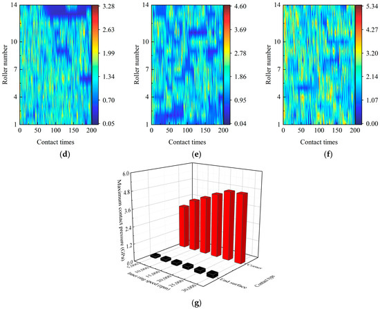
Figure 9. Contact pressure between the roller arc end surface and the flange at the inner-ring speed of (a) 5000 rpm, (b) 15,000 rpm, and (c) 30,000 rpm, and that between the roller corner and the flange at the inner ring speed of (d) 5000 rpm, (e) 15,000 rpm, (f) 30,000 rpm, and (g) maximum contact pressure.

Figure 10 shows the sliding velocity between the arc end surface of the roller or roller corner and the flange (|${\mathbf{u}}_{\mathbf{brf}}^{\mathbf{rf}}$| and |${\mathbf{u}}_{\mathbf{berf}}^{\mathbf{rf}}$|) by considering different inner-ring speeds $n_{\mathrm{i}}$. Figure 10a–f are the sliding velocities between different rollers and flanges within 200 contact times by considering various $n_{\mathrm{i}}$. Figure 10g represents the peak value of (|${\mathbf{u}}_{\mathbf{brf}}^{\mathbf{rf}}$| and |${\mathbf{u}}_{\mathbf{berf}}^{\mathbf{rf}}$|) with various $n_{\mathrm{i}}$. |${\mathbf{u}}_{\mathbf{brf}}^{\mathbf{rf}}$| reaches 3.83 m/s (Figure 10a), 11.02 m/s (Figure 10b), and 21.38 m/s (Figure 10c) as $n_{\mathrm{i}}$ is 5000 rpm, 15,000 rpm, and 30,000 rpm, respectively. This means the |${\mathbf{u}}_{\mathbf{brf}}^{\mathbf{rf}}$| increases linearly with the increase in $n_{\mathrm{i}}$, and this trend is also observed when the roller corner contacts the flange (Figure 10d–f). However, |${\mathbf{u}}_{\mathbf{brf}}^{\mathbf{rf}}$| is much larger than |${\mathbf{u}}_{\mathbf{berf}}^{\mathbf{rf}}$| (Figure 10d–g), especially when $n_{\mathrm{i}}$ is 30,000 rpm (Figure 10f).

Figure 10. Sliding velocity between the roller arc end surface and the flange at the inner-ring speed of (a) 5000 rpm, (b) 15,000 rpm, and (c) 30,000 rpm, and that between the roller corner and the flange at the inner ring speed of (d) 5000 rpm, (e) 15,000 rpm, (f) 30,000 rpm, and (g) maximum sliding velocity.

Figure 11 shows the PV value between the arc end surface of the roller or roller corner and the flange ($P{V}_{\mathrm{brf}}$ and $P{V}_{\mathrm{berf}}$) by considering different inner-ring speeds $n_{\mathrm{i}}$. Figure 11a–f are the PV values between different rollers and flanges within 200 contact times by considering various $n_{\mathrm{i}}$. Figure 11g represents the peak ($P{V}_{\mathrm{brf}}$ and $P{V}_{\mathrm{berf}}$) with various $n_{\mathrm{i}}$. As $n_{\mathrm{i}}$ increases from 5000 rpm to 30,000 rpm, $P{V}_{\mathrm{brf}}$ between the arc end surface of the roller and the flange increases from 0.53 GPa·m/s (Figure 11a) to 5.12 GPa·m/s (Figure 11c). This trend is also observed when the roller corner contacts the flange, and the peak $P{V}_{\mathrm{brf}}$ reaches 147 GPa·m/s if $n_{\mathrm{i}}$ arrives at 30,000 rpm (Figure 11f). This is because of the combined increase in p_brf,max and the sliding speed |${\mathbf{u}}_{\mathbf{berf}}^{\mathbf{rf}}$|. However, compared to the contact between the roller corner and the flange, PV values decrease obviously if the arc end surface of the roller is adopted (Figure 11g).

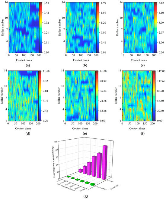
Figure 11. PV value between the roller arc end surface and the flange at the inner-ring speed of (a) 5000 rpm, (b) 15,000 rpm, and (c) 30,000 rpm, and that between the roller corner and the flange at the inner-ring speed of (d) 5000 rpm, (e) 15,000 rpm, (f) 30,000 rpm, and (g) maximum PV value.

The effect on the sliding velocity |${\mathbf{u}}_{\mathbf{berf}}^{\mathbf{rf}}$| and the PV value $P{V}_{\mathrm{berf}}$ between the roller and the flange by considering different end radii of the roller $R_{\mathrm{end}}$ and layback angles of the flange ${\mathsf{\theta }}_{\mathrm{rrf}}^{\mathrm{r}}$ is shown in Figure 12 (inner-ring speed $n_{\mathrm{i}}$ of 20,000 rpm and radial load $F_{\mathrm{z}}^{\mathrm{I}}$ of 1000 N). As $R_{\mathrm{end}}$ increases from 80 mm to 110 mm, |${\mathbf{u}}_{\mathbf{berf}}^{\mathbf{rf}}$| rises significantly (Figure 12a). However, $P{V}_{\mathrm{berf}}$ between the roller and the flange decreases slightly. If ${\mathsf{\theta }}_{\mathrm{rrf}}^{\mathrm{r}}$ increases from 1.5° to 1.8°, |${\mathbf{u}}_{\mathbf{berf}}^{\mathbf{rf}}$| rises from 14 m/s to 16.5 m/s (Figure 12b). Meanwhile, $P{V}_{\mathrm{berf}}$ decreases first and then increases.

Figure 12. Sliding velocity and PV value between the roller and the flange with consideration of different (a) end radii of the roller and (b) layback angles of the flange.

Figure 13 shows the contact position on the roller end surface in the radial (y and z) directions with consideration of different layback angles of the flange ${\mathsf{\theta }}_{\mathrm{rrf}}^{\mathrm{r}}$, end radii of the roller $R_{\mathrm{end}}$, and central lengths of the roller $L_{\mathrm{b}2}$. The inner-ring speed ${\mathrm{n}}_{\mathrm{i}}$ is set to 20,000 rpm, and the radial load $F_{\mathrm{z}}^{\mathrm{I}}$ is set to 1000 N. The limited circle is the critical value for avoiding contact between the roller corner and the flange when the roller end surface has a circular arc. Figure 13a shows the effect of ${\mathsf{\theta }}_{\mathrm{rrf}}^{\mathrm{r}}$ on the contact position on the end surface of the roller. $R_{\mathrm{end}}$ is set to 80 mm, and $L_{\mathrm{b}2}$ is set to 4.5 mm. As ${\mathsf{\theta }}_{\mathrm{rrf}}^{\mathrm{r}}$ increases from 1.5° to 1.8°, the contact radius is somewhat increased and scattered. This means that to make the contact trajectory on the roller end surface more concentrated, ${\mathsf{\theta }}_{\mathrm{rrf}}^{\mathrm{r}}$ should be reduced as much as possible. Otherwise, the contact surface position may be out of the arc end surface of the roller. Figure 13b shows the effect of $R_{\mathrm{end}}$ on the contact position on the end surface of the roller. ${\mathsf{\theta }}_{\mathrm{rrf}}^{\mathrm{r}}$ is set to 1.6°, and $L_{\mathrm{b}2}$ is set to 4.5 mm. The contact position distribution on the roller increases as the radius rises and is close to the limited circle. Notably, when $R_{\mathrm{end}}$ is set to 1 × 10¹⁰ mm, i.e., the flange contacts the roller corner, the contact position distribution on the roller equals the limited circle. Therefore, in $R_{\mathrm{end}}$ design, to prevent an increase in the contact track radius on the roller end surface, $R_{\mathrm{end}}$ should be reduced. Figure 13c shows the effect of $L_{\mathrm{b}2}$ on the contact position on the end surface of the roller. As $L_{\mathrm{b}2}$ decreases from 6.5 mm to 0.5 mm, the contact location distribution becomes dispersed. This is caused by the fact that the roller is more prone to misalignment and skew in the raceways of rings due to the reduction in $L_{\mathrm{b}2}$.

Figure 13. Contact position on the roller along the radial (y and z) direction with consideration of different layback angles of the flange, end radius of the roller, and central lengths of the roller at (a) effect of layback angle of the flange, (b) effect of end radius of the roller, and (c) effect of roller central length.

Figure 14a demonstrates the limit range on the end radius of the roller $R_{\mathrm{end}}$ and the layback angle of the flange ${\mathsf{\theta }}_{\mathrm{rrf}}^{\mathrm{r}}$ by considering the contact height between the roller and the flange. The initial height of the flange $H_{\mathrm{rf}}$ is 2 mm. The upper limit line is aimed at making sure that the contact area is in the range of $H_{\mathrm{rf}}$ and is set to 1.8 mm. The lower limit line is aimed at making sure that the edge of the contact area does not fall at the base of the flange. As $R_{\mathrm{end}}$ or ${\mathsf{\theta }}_{\mathrm{rrf}}^{\mathrm{r}}$ decreases, the contact height obviously increases. This means that $H_{\mathrm{rf}}$ needs to be increased to make sure that the contact height falls into the green zone by the smaller $R_{\mathrm{end}}$ and ${\mathsf{\theta }}_{\mathrm{rrf}}^{\mathrm{r}}$. Figure 14b demonstrates the limit range of $R_{\mathrm{end}}$ and ${\mathsf{\Delta }}_{\mathrm{bf}}$ by considering actual clearance ${\mathsf{\Lambda }}_{\mathrm{bf}}$. The contact line is aimed at making sure that ${\mathsf{\Lambda }}_{\mathrm{bf}}$ under axial direction is larger than 0 mm. If ${\mathsf{\Lambda }}_{\mathrm{bf}}$ is less than 0 mm, the flange contacts the roller at the initial time. As $R_{\mathrm{end}}$ decreases, ${\mathsf{\Delta }}_{\mathrm{bf}}$ needs to be increased to overcome the contact line. However, the range of options for ${\mathsf{\Delta }}_{\mathrm{bf}}$ selection is significantly expanded by the larger $R_{\mathrm{end}}$.

Figure 14. Influence of the (a) contact height on the end radius of the roller and the layback angle of the flange and (b) actual clearance on the end radius of the roller and the axial clearance.

4. Validations

The accuracy of the roller/raceway contact simulation is demonstrated via validation in Figure 10 of Ref. [22] and indicates a high degree of coincidence. In addition, to validate the fitness of the dynamic model for the bearing analyzed, the cage speed $n_{\mathrm{c}}$ of the bearing used in the analysis is tested and compared with the results of the dynamic model to verify its accuracy.

As illustrated in Figure 15, the test equipment comprises a motor drive, an increasing gearbox, a junction box, a lubrication system, a bearing housing, and a slip ring for signal transmission. The cage speed $n_{\mathrm{c}}$ was measured using a reflective optical fiber sensor positioned adjacent to the cage end face (approximately 3 mm × 3 mm detection area), which captured pulse signals corresponding to rotational motion. A LabVIEW-based data acquisition system processed these signals, enabling a real-time display and recording of $n_{\mathrm{c}}$. The oil for lubrication is 4106 while the temperature of the oil supply is 80 °C. The dynamic viscosity, pressure–viscosity coefficient, and temperature–viscosity coefficient are 0.055 Pa·s, 1.85 × 10⁻⁸ Pa⁻¹, and 0.0315 °C⁻¹, respectively.

Figure 15. Schematic diagram of the test rig for measuring the cage speed.

An optical fiber sensor (model FS-V31, KEYENCE, Osaka, Japan) was used to capture the cage speed, and its characteristics of small size and fast response are suitable for measurement in the bearing structure size limitation and the high-speed cage. Reflection marker areas were prepared on the side of the cage, and the reflected light signal due to the rotation of the cage was converted into a pulse signal. Six power modes were available for the optical fiber sensor. The fastest response time was only 0.033 ms under the HIGH-SPEED mode, and the corresponding limit frequency was 30 KHz, which means the maximum theoretical measurement limit was 1.8M rpm, which can fully cover the range of cage speed testing. A pulse counter (model XSM, Harbin, China) was used to supply DC power for the sensor and convert pulse signals into rotational speed. Its measurement frequency is up to 25kHz, and the basic error is ± 0.02%FS. The speed information was submitted to the LabVIEW-based data acquisition system via VISA serial communication. The experimental process is as follows: when conducting the test, first start the test bench to ensure that all systems are stable. Then gradually increase the load to the tested condition and increase the inner-ring speed $n_{\mathrm{i}}$. The duration of this process is automatically controlled by the gearbox system. Then, at each operating condition, a 6 min stay is conducted, and the data from the last 5 min are processed to ensure the stability of the bearing condition. After running all the test load curves, reduce the rotational speed to 0 rpm and then unload and shut down.

Figure 16 shows the cage speed $n_{\mathrm{c}}$ from the model in this paper and the experiments using the test rig (Figure 15). The errors are also presented in Figure 14. Since the maximum error between the model and the experiment is less than 2.7% (Figure 16c), the accuracy of the model has been verified.

Figure 16. Comparison between theoretical and practical values of the cage speed at inner-ring speed equaling (a) 4000 rpm, (b) 8000 rpm, and (c) 12,000 rpm.

5. Conclusions

A novel interference model between the arc end surfaces of rollers and the flanges of rings is proposed and integrated into the dynamic model of cylindrical roller bearings. Dynamic behaviors, i.e., contact pressures, sliding velocities, and PV values, are investigated and compared to those between roller corners and flanges. Through the research, the primary advantage of this model is the reduction in contact pressures, sliding velocities, and PV values at the roller–flange interface, particularly under high-speed conditions. Due to the change in the roller structure, the end radius of the roller, the central length of the roller, and the layback angle of the flange also affect dynamic behaviors. This is mainly because the contact position between the roller and the flange is changed. The following conclusions are obtained:

• The contact pressure between the arc end surface and the flange is reduced as the contact radius is larger than that between the roller corner and the flange. Consequently, the PV value also decreased, especially for high-speed conditions.
• The sliding velocity abates obviously while the end radius of the roller as well as the layback angle of the flange decrease. Meanwhile, the contact positions on the roller end surface are more concentrated with a smaller radius of contact points to the origin. The peak value of the PV value between the arc end surface of the roller and the flange increases slightly as the end radius of the roller decreases.
• The flange height needs to be increased to avoid the contact height on the flange being overtop while decreasing the end radius of the roller and the layback angle of the flange. In addition, the axial clearance of the flange needs to be relaxed to avoid initial contact between the roller and the flange, since the arc of the end surface further extends the length of the rollers.

References

- Bao, M.; Wang, L.; Niu, K.; Zheng, D.; Zhang, C. Dynamic behavior analysis of cylindrical roller bearings with trilobe outer raceway: Effect of the out-of-roundness, phase angle and initial clearance. Tribol. Int. 2025, 204, 110498. [Google Scholar] [CrossRef]
- Gupta, P.K. Dynamics of rolling-element bearings—Part I: Cylindrical roller bearing analysis. J. Lubr. Technol. 1979, 101, 293–302. [Google Scholar] [CrossRef]
- Gupta, P.K. Dynamics of rolling-element bearings—Part II: Cylindrical roller bearing results. J. Lubr. Technol. 1979, 101, 305–311. [Google Scholar] [CrossRef]
- Gupta, P.K. Dynamics of rolling-element bearings—Part III: Ball bearing analysis. J. Lubr. Technol. 1979, 101, 312–318. [Google Scholar] [CrossRef]
- Gupta, P.K. Dynamics of rolling-element bearings—Part IV: Ball bearing results. J. Lubr. Technol. 1979, 101, 319–326. [Google Scholar] [CrossRef]
- Hu, Y.; He, L.; Luo, Y.; Tan, A.C.; Yi, C. Contact load calculation models for finite line contact rollers in bearing dynamic simulation under dry and lubricated conditions. Lubricants 2025, 13, 183. [Google Scholar] [CrossRef]
- Zhou, R.; Li, M.; Liu, H.; Pan, W.; Zhang, R.; Liu, Y. Theoretical and experimental study on the evolution of contact load during wear failure of cylindrical roller bearings. Eng. Fail. Anal. 2025, 169, 109218. [Google Scholar] [CrossRef]
- Kabus, S.; Hansen, M.R.; Mouritsen, O.Ø. A new quasi-static cylindrical roller bearing model to accurately consider non-hertzian contact pressure in time domain simulations. J. Tribol. 2012, 134, 041401. [Google Scholar] [CrossRef]
- Qiu, L.; Liu, S.; Chen, X.; Wang, Z. Lubrication and loading characteristics of cylindrical roller bearings with misalignment and roller modifications. Tribol. Int. 2022, 165, 107291. [Google Scholar] [CrossRef]
- Bogdan, W.; Agnieszka, C. Effect of ring misalignment on the fatigue life of the radial cylindrical roller bearing. Int. J. Mech. Sci. 2016, 111–112, 1–11. [Google Scholar] [CrossRef]
- Ye, Z.; Wang, L.; Gu, L.; Zhang, C. Effects of tilted misalignment on loading characteristics of cylindrical roller bearings. Mech. Mach. Theory 2013, 69, 153–167. [Google Scholar] [CrossRef]
- Tian, J.; Wang, P.; Xu, H.; Ma, H.; Zhao, X. Nonlinear vibration characteristics of rolling bearing considering flexible cage fracture. Int. J. Non Linear Mech. 2023, 156, 104478. [Google Scholar] [CrossRef]
- Wang, H.; Li, Z.; Ji, X.; Wang, C.; Yang, L. Cage stability analysis of mixed-mounted double row angular contact ball bearing. Mech. Mach. Theory 2025, 211, 106035. [Google Scholar] [CrossRef]
- Tu, W.; Liang, J.; Yu, W.; Shi, Z.; Liu, C. Motion stability analysis of cage of rolling bearing under the variable-speed condition. Nonlinear Dyn. 2023, 111, 11045–11063. [Google Scholar] [CrossRef]
- Chen, H.; Zhang, H.; Liang, H.; Wang, W. The collision and cage stability of cylindrical roller bearing considering cage flexibility. Tribol. Int. 2024, 192, 109219. [Google Scholar] [CrossRef]
- Harsha, S.P.; Kankar, P.K. Stability analysis of a rotor bearing system due to surface waviness and number of balls. Int. J. Mech. Sci. 2004, 46, 1057–1081. [Google Scholar] [CrossRef]
- Ren, Z.; Wang, J.; Guo, F.; Lubrecht, A. Experimental and numerical study of the effect of raceway waviness on the oil film in thrust ball bearings. Tribol. Int. 2014, 73, 1–9. [Google Scholar] [CrossRef]
- Liu, J.; Shao, Y. Vibration modelling of nonuniform surface waviness in a lubricated roller bearing. J. Vib. Control. 2017, 23, 1115–1132. [Google Scholar] [CrossRef]
- Niu, L. A simulation study on the effects of race surface waviness on cage dynamics in high-speed ball bearings. J. Tribol. 2019, 141, 051101. [Google Scholar] [CrossRef]
- Mao, Y.; Wang, L.; Zhang, C. Study on the load distribution and dynamic characteristics of a thin-walled integrated squirrel-cage supporting roller bearing. Appl. Sci. 2016, 6, 415. [Google Scholar] [CrossRef]
- Tu, W.; Yu, W.; Shao, Y.; Yu, Y. A nonlinear dynamic vibration model of cylindrical roller bearing considering skidding. Nonlinear Dyn. 2021, 103, 2299–2313. [Google Scholar] [CrossRef]
- Bao, M.; Wang, L.; Wang, J.; Zhang, C. Slipping in cylindrical roller bearings at the simultaneous rotation of inner and outer rings. Tribol. Int. 2024, 197, 109767. [Google Scholar] [CrossRef]
- Deng, S.; Liu, Y.; Zhang, W.; Sun, X.; Lu, Z. Cage slip characteristics of a cylindrical roller bearing with a trilobe-raceway. Chin. J. Aeronaut. 2018, 31, 351–362. [Google Scholar] [CrossRef]
- Liu, Y.; Chen, Z.; Tang, L.; Zhai, W. Skidding dynamic performance of rolling bearing with cage flexibility under accelerating conditions. Mech. Syst. Signal Process. 2021, 150, 107257. [Google Scholar] [CrossRef]
- Liu, Y.; Chen, Z.; Li, Y.; Zhai, W. Dynamic investigation and alleviative measures for the skidding phenomenon of lubricated rolling bearing under light load. Mech. Syst. Signal Process. 2023, 184, 109685. [Google Scholar] [CrossRef]
- Wang, Z.; Lv, X.; Song, J. Tolerance analysis of cylindrical roller bearing under combined radial and axial loads. Math. Probl. Eng. 2022, 1, 9233627. [Google Scholar] [CrossRef]
- Wolf, M.; Sanner, A.; Fatemi, A. A semi-analytical approach for rapid detection of roller-flange contacts in roller element bearings. Proc. Inst. Mech. Eng. Part J J. Eng. Tribol. 2020, 235, 1440–1449. [Google Scholar] [CrossRef]
- Bayrak, R.; Sagirli, A. Fatigue life analysis of the radial cylindrical roller bearings: Roller end-flange construction effect. Mech. Based Des. Struct. Mach. 2022, 51, 7030–7055. [Google Scholar] [CrossRef]
- Hou, X.; Diao, Q.; Liu, Y.; Liu, C.; Zhang, Z.; Tao, C. Failure analysis of a cylindrical roller bearing caused by excessive tightening axial force. Machines 2022, 10, 322. [Google Scholar] [CrossRef]
- Gupta, P.K. Advanced Dynamics of Rolling Elements; Springer: New York, NY, USA, 1984. [Google Scholar]
- Pauli, V.; Ralf, G.; Oliphant, T.E.; Haberland, M.; Reddy, T.; Cournapeau, D.; Burovski, E.; Peterson, P.; Weckesser, W.; Bright, J.; et al. SciPy 1.0: Fundamental algorithms for scientific computing in python. Nat. Methods 2020, 17, 261–272. [Google Scholar]
Disclaimer/Publisher’s Note: The statements, opinions and data contained in all publications are solely those of the individual author(s) and contributor(s) and not of MDPI and/or the editor(s). MDPI and/or the editor(s) disclaim responsibility for any injury to people or property resulting from any ideas, methods, instructions or products referred to in the content. |
© 2025 by the authors. Licensee MDPI, Basel, Switzerland. This article is an open access article distributed under the terms and conditions of the Creative Commons Attribution (CC BY) license (https://creativecommons.org/licenses/by/4.0/).