Bearing Fault Diagnosis via Incremental Learning Based on the Repeated Replay Using Memory Indexing (R-REMIND) Method

Abstract

In recent years, deep-learning schemes have been widely and successfully used to diagnose bearing faults. However, as operating conditions change, the distribution of new data may differ from that of previously learned data. Training using only old data cannot guarantee good performance when handling new data, and vice versa. Here, we present an incremental learning scheme based on the Repeated Replay using Memory Indexing (R-REMIND) method for bearing fault diagnosis. R-REMIND can learn new information under various working conditions while retaining older information. First, we use a feature extraction network similar to the Inception-v4 neural network to collect bearing vibration data. Second, we encode the features by product quantization and store the features in indices. Finally, the parameters of the feature extraction and classification networks are updated using real and reconstructed features, and the model did not forget old information. The experiment results show that the R-REMIND model exhibits continuous learning ability with no catastrophic forgetting during sequential tasks.

1. Introduction

Rolling element bearings play vital roles in mechanical equipment. About 40% of all large mechanical system failures, and 90% of those of small rotating machines, are caused by bearing defects [1]. Bearings support rotating bodies to reduce friction and guarantee rotational accuracy [2]. Bearings normally work in complex and harsh conditions. They are prone to failure that shuts down the entire machine. Bearing monitoring and diagnosis ensure safety and reduce economic losses. In recent years, various types of signals have been used for bearing faults diagnosis, including vibration [3,4,5,6,7], the stator current [8,9], acoustic emissions [10,11], and thermal images [12]. Traditional diagnostic methods are effective when there are few data. They can extract and study features and make decisions using pattern recognition algorithms. However, traditional methods are slow when the dataset is extensive [13]. Deep-learning schemes have thus been used to diagnose bearing faults [14,15,16]. Pham et al. [17] used the constant-Q transform technique to transform acoustic emission signals into spectrographic images that served as inputs to a convolutional neural network (CNN) multiple-output model. He et al. [18] presented a deep transfer-learning method based on a one-dimensional (1D) CNN, which was highly successful under various conditions. CNNs accept diverse input data, allow easy adjustment of network structure, and generalize very effectively [19]. Compared to a two-dimensional (2D)-CNN, a 1D-CNN can directly identify bearing data for more efficient performance of end-to-end tasks.

Given the complex and changeable bearing work environments, the distributions of collected data vary greatly. As deep-learning algorithms are generally data-driven, diagnostic accuracy may decrease when the data distribution changes. This is termed catastrophic forgetting; the model forgets old information after acquiring new information, which severely compromises diagnostic performance. When the work conditions vary continuously, it is essential to retrain the model using new data to ensure diagnostic accuracy. However, this repetitive training imposes a burden and it is impossible to store historical data or trained models. Incremental learning can handle this problem. Regarding bearing fault diagnosis, incremental learning methods including class incremental learning [20,21,22,23] and imbalanced data learning [24,25] have been developed. However, few studies have focused on catastrophic forgetting. Li et al. [26] presented an incremental learning method based on a layer regeneration network; distillation loss was used to alleviate catastrophic forgetting and the results were satisfactory. Continuous learning from bearing failures was more effective than fine-turning and joint-training methods. However, if old data are unavailable because of privacy issues or other concerns, model accuracy may be very poor. To address this problem, we present a bearing fault diagnosis method based on a 1D CNN and product quantization; i.e., the Repeated Replay using Memory Indexing (R-REMIND) model. We were inspired by the REMIND incremental learning algorithm of Hayes et al. [27]. The R-REMIND model is like a brain that learns new information repeatedly, as opposed to only once. The model uses a feature extraction module based on a simplified 1D Inception-ResNet network to extract features from raw bearing vibration data. The features are encoded via product quantization and the codes are stored in buffer indices. A classification network identifies the fault type. When encountering new data, the model decodes the stored code and replays the reconstructed features, together with the real features of the new task, to update the parameters of the feature extraction and classification networks.

The contribution of this study is summarized as follows: We use a brain-inspired bearing diagnostic method for bearing fault diagnosis to enhance learning of new tasks and prevent performance degradation when performing old tasks. The old data are not needed during training with new data. Meanwhile, the proposed method might greatly reduce training time. The proposed method is more accurate and presents good ability in not forgetting old information.

The rest of the paper is organized as follows. Section 2 provides the theoretical background, Section 3 describes and applies the method, Section 4 details the experiments, and Section 5 concludes the study.

2. Theoretical Background

2.1. Inception-ResNet Module

He et al. [28] designed a residual block with a shortcut based on CNN, which facilitated optimization and eliminated the gradient vanishing, gradient explosion, and network degradation associated with increased network depth. Subsequently, Szegedy et al. [29] improved this model when developing the Inception-ResNet network; the basic module is shown in Figure 1. Convolutional layers with kernels of different sizes are concatenated into a single output vector (an inception block) that learns residual information $F\left(x\right)$ from input $x$. The shortcut adds input $x$ to the residual result $F\left(x\right)$ to enable mapping $H\left(x\right)$. The Inception-v4 framework of [29] has three types of inception blocks with diverse convolutional layers that capture information from different dimensions. The shortcut connection retains the advantages of residual networks.

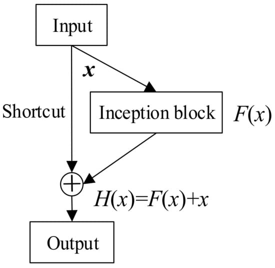
Figure 1. General schema of Inception-ResNet modules.

2.2. Product Quantization

Quantization is a destructive process extensively studied by information theorists. The aim is to reduce the cardinality of the representation space when input data are real-valued [30]. Formally, a quantizer is a function $q$ mapping a D-dimensional vector $x\in {ℝ}^D$ to a vector $q\left(x\right)\in \complement =\left\{c_i;i\in {\rm I}\right\}$, where the index set ${\rm I}$ is assumed to be finite: ${\rm I}=0\dots k-1$. The set of reproduction values $\complement$ is a codebook of size $k$, and the reproduction values $c_i$ are centroids. However, as the value of $k$ increases, it becomes too difficult to use the Lloyd algorithm to quantize the vectors, and it is unrealistic to store the $D\times k$ floating point values representing the $k$ centroids. Product quantization efficiently addresses these issues. The space is decomposed into a Cartesian product of low-dimensional subspaces that are separately quantized [30]. The input data are split into $m$ distinct subvectors $u_j$ of dimension $D^{*}=D/m$, where $1\le j\le m$ and D is a multiple of $m$. The subvectors are quantized using $m$ distinct quantizers. A given vector $x$ is mapped as:

$$\underset{u_1(x)}{\underbrace{x_1,\dots ,x_{D*}}},\dots ,\underset{u_m(x)}{\underbrace{x_{D-D*+1},\dots x_D}}\to q_1(u_1(x)),\dots ,q_m(u_m(x))$$

(1)

The product index set $I$ is defined as the Cartesian product of the index sets of the subquantizers:

$$I=I_1\times \dots \times I_m$$

(2)

Similarly, the product codebook $C$ is defined as:

$$C=C_1\times \dots \times C_m$$

(3)

A reproduction value is a concatenation of the $m$ centroids of the corresponding subquantizers, identified by an element of the product index set $I$. If all subquantizers have the same finite number $k^{*}$ of reproduction values, the total number of product centroids is:

$$k={(k^{*})}^m$$

(4)

Thus, product quantization produces a large set of centroids from several small sets of centroids associated with the subquantizers. Therefore, a vector is represented by a short code composed of subspace quantization indices. To satisfy the optimal Lloyd conditions, the k-means clustering algorithm can be applied to learn the subquantizers [30].

3. The Proposed Method

3.1. The R-REMIND Model

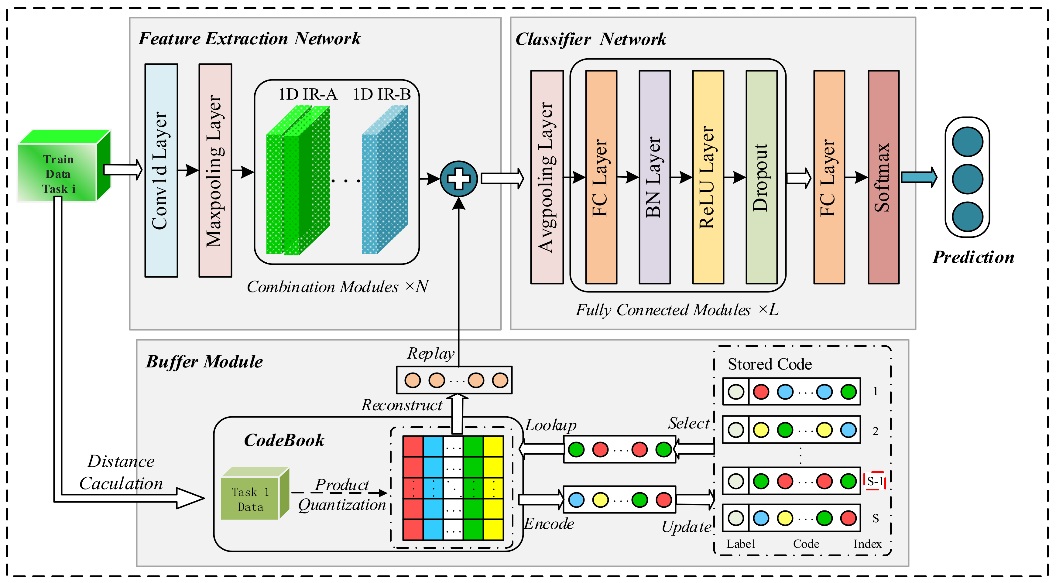
The architecture of our proposed R-REMIND model, which is based on the work of Hayes et al. [27], is shown in Figure 2. It consists of three parts: a feature extraction network, classification network, and buffer module. The feature extraction network is composed mainly of combination modules, each of which is a stack of several 1D inception reduction (IR)-A modules and one 1D IR-B module. The features of 1D bearing vibration signals are extracted. The classification network contains several fully connected modules, each of which consists of a fully connected layer, a batch normalization (BN) layer, a ReLU activation layer, and a dropout layer. The classification network learns the features of current data and the reconstructed features and classifies the real features to aid diagnosis. The buffer module encodes the extracted features and stores them in indices. Stored code representing historical data is decoded and replayed during continuous data learning.

Figure 2. Architecture of the R-REMIND model.

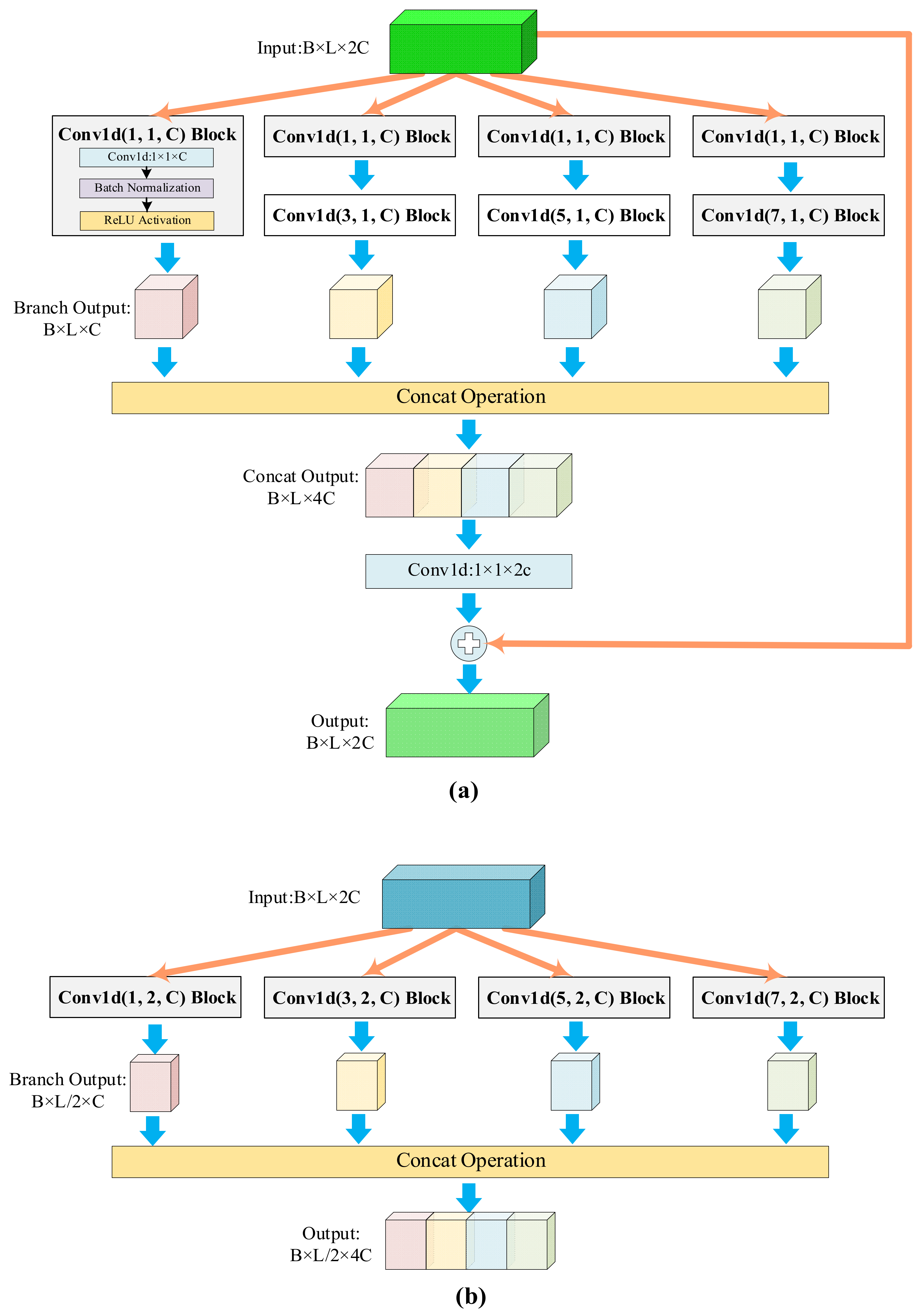
The feature extraction network has a convolutional layer, max-pooling layer, and $N$ combination modules. As the inputs are segments of 1D time series signals, the data point with damage information may have a relationship with the data that appear far away from it. Thus, a convolutional layer and max-pooling layer (with a larger kernel) are used to acquire more defect knowledge. The combination module is composed of a few 1D IR-A modules followed by one 1D IR-B module (Figure 3). Both modules are based on 1D convolutional blocks (“Conv1d Block” in the figure) that contain sequential convolution, BN, and ReLU activation layers. The block parameters are the same as for the convolutional layer. The three parameters represent the kernel size, stride, and number of the convolutional layer. Equation (5) shows the receptive field relationships among a stack of several convolutional layers, where $F^i$ is the field of the $i$th layer and $s$ and $ks$ are the stride and kernel size of the convolutional layer, respectively:

$$F^i=(F^{i+1}-1)\times s+ks$$

(5)

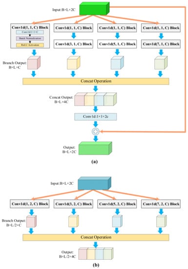
Figure 3. The 1D-Inception-ResNet modules. (a) The 1D IR-A module. (b) The 1D IR-B module.

The definition of a receptive field indicates that a stack of two $3\times 3$ convolutional layers provides an effective receptive field of $5\times 5$. Three such layers have a receptive field of $7\times 7$[31]. When several small 2D convolutional layers are used, the number of model parameters is decreased. However, the opposite is true when using 1D CNN models. Taking the $7\times 1$ convolutional layer as an example, the receptive field is $7\times 1$, which is the same as that of a stack of three 3$\times 1$ convolutional layers. The former model has fewer parameters than the latter. We thus use multiple convolutional layers of different kernel sizes, and do not stack several small convolutional layers in each branch. To facilitate model hyperparameter adjustment, we set the output channel of the 1D convolutional block to half that of the input channel. The 1D IR-A module is mainly used to deepen the network structure and increase complexity; the shortcut connection retains the advantages of the ResNet network architecture. The 1D IR-B module performs feature extraction and compression. The two types of 1D-Inception-ResNet modules capture the information in different dimensions, thus improving feature extraction.

The classification network of R-REMIND is a traditional neural network with an average pooling layer, several fully connected modules, a fully connected layer for final classification, and a Softmax layer. The fully connected module includes BN, ReLU activation, and dropout layers (Figure 3), and jointly learns both current and reconstructed features. Real features from the extraction network are used for diagnosis. The loss function is the negative log-likelihood function:

$$NLLLoss=-{\displaystyle \sum _{i=1}^m\log (P(x^i;\theta ))}$$

(6)

where $m$ is the number of samples and $P\left(x^i;\theta \right)$ is the probability that the predicted feature $x^i$ occurs in the classification network for parameter $\theta$.

The buffer module shown in Figure 3 has two working states. It handles either first-task data or other-task data. When R-REMIND learns first-task data, there is no code in the buffer. Thus, the buffer module splits the features extracted from the current data into subvectors, uses the k-means clustering algorithm to quantize these data individually to obtain the codebook $C$, and stores the learned centroids. Therefore, we achieved product quantization. In other situations, the buffer module randomly selects stored code using an index and reconstructs features by reference to that code and the stored centroids. The buffer module thus provides both reconstructed and real features when the networks update the parameters. Additionally, the buffer module updates the stored code during continuous learning. It encodes real features by calculating the distances between subvectors and the corresponding centroids. The code with labels is stored in the buffer after the model finishes learning a task.

3.2. Diagnostic Framework

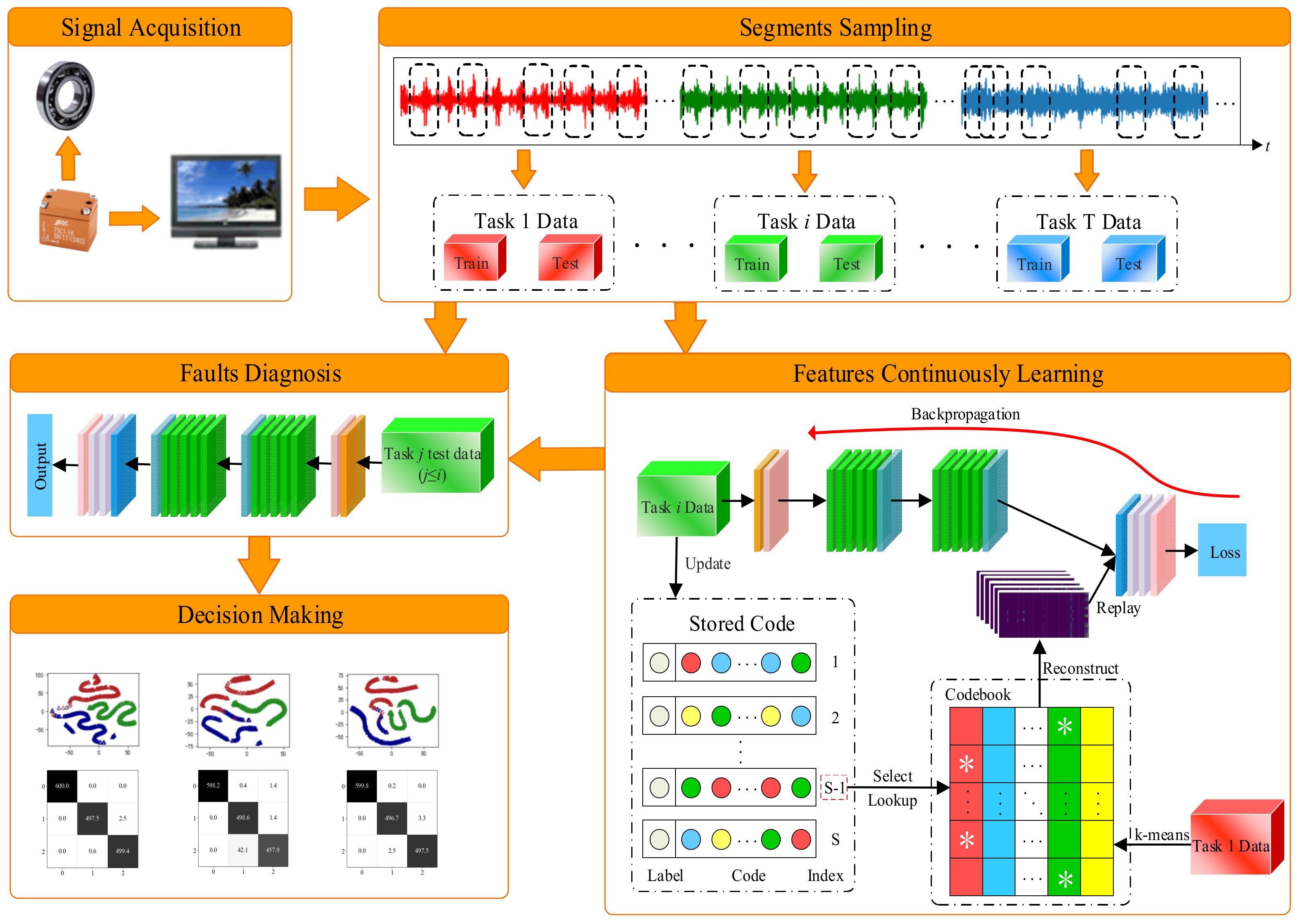
Our novel diagnostic model combines a 1D-Inception-ResNet network with product quantization. The model continuously learns bearing vibration signals under various working conditions and diagnoses faults. The framework of the R-REMIND model is illustrated in Figure 4. The procedure is listed as follows:

• Step 1: Signal acquisition. Under different loads, vibration signals and bearing status data are collected and processed.
• Step 2: Segmental sampling. The collected raw vibration signals are randomly sampled using a fixed-length sliding window. The sampled segments are divided into training and test datasets under various working conditions.
• Step 3: Continuous learning. The training data for different tasks are sequentially learned by R-REMIND. The buffer module is updated using the features of the current task after learning is complete.
• Step 4: Fault diagnosis. The data of previous tasks are diagnosed by the current R-REMIND model to verify the effectiveness of the method.
• Step 5: Decision-making. The model reviews the bearing status and developmental trend, and then makes a decision.

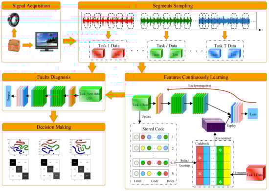
Figure 4. Framework of our proposed diagnostic method.

Figure 4. Framework of our proposed diagnostic method.

4. Experiments and Results

4.1. The Dataset

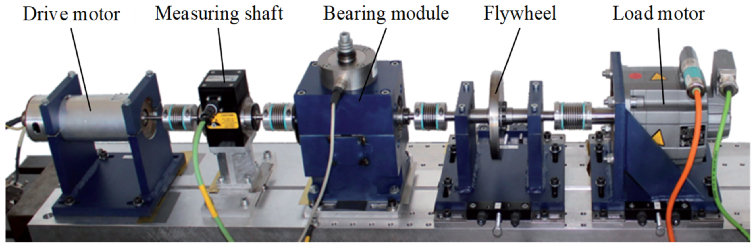
The performance of R-REMIND was assessed using a dataset from Paderborn University [32]. The dataset was derived using ball bearings of type 6203 and includes information on artificial damage caused by electric discharge machining, drilling, and electric engraving, as well as real damage caused by a bearing accelerated lifetime test apparatus driven by an electric asynchronous motor. A constant radial load is applied to the box, and can be adjusted using a spring and a nut. Four bearings can be tested simultaneously. Each bearing operates under constant load until damage occurs. The bearings present typical types of damage. Bearing faults include inner, outer, and mixed race faults, which are divided into three fault levels according to the extent of the damage. The experimental data are vibration signals obtained by running the test rig shown in Figure 5 at 64 kHz for 4 s. The operating conditions can be varied by changing the speed of the drive motor, turning the adjusting nut on the bearing module, or varying the current of the load motor.

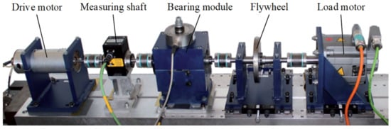
Figure 5. The Paderborn University test rig providing bearing fault data.

To verify the effectiveness of our method, the vibration data under various working conditions were continuously and sequentially learned (Table 1). Each task provides vibration data for three states, i.e., healthy bearings and bearings with inner and outer race faults. The bearing codes for the simulation are listed in Table 2. As the vibration datasets collected during one bearing rotation comprise 2560 data points, the sampling sliding window length was set to 2560. To ensure that all samples were collected when the bearings were stable, we discarded the first and last 10% of samples (the data length thus became 3.2 s). The random sampling method (Figure 6) ensured that the samples were diverse and accurate. Five hundred samples were randomly obtained from each bearing code, and each task contained 8000 samples that were randomly divided into training, validation, and test datasets in a 6:2:2 ratio.

Table 1. Bearing operational parameters.

Task	Rotation Speed (r/min)	Load Torque (N·m)	Radial Force (N)
1	1500	0.1	1000
2	1500	0.7	400
3	1500	0.7	1000

Table 2. Bearing codes (different classes).

Healthy	Inner Race Fault	Outer Race Fault
K001, K002, K003 K004, K005, K006	KI04, KI14, KI17, KI18 KI21	KA04, KA15, KA16, KA22, KA30

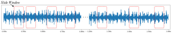
Figure 6. Schematic of the sampling process.

4.2. Experimental Setup

During training, the dropout ratio (drs) of the dropout layer is set to 0.5. The number (m) and size of the codebooks (k) are set to 32 and 256, respectively (Jegou et al. [30]) and the size of the buffer module (BS) is set to 10,000. The batch size (bs) is set to 128; the number of training epochs is 300. The Adam optimizer is applied, and the weight decay ratio (wd) is set to 10⁻⁵. The replay ratio (rr) is set to 1, which means that the number of reconstructed features is equal to the number of real features. The remaining parameters are determined by random searching. The final model hyperparameters are listed in Table 3, where in row 4, 0 is the 1D IR-A module and 1 is the 1D IR-B module.

Table 3. The hyperparameters of R-REMIND.

Parameter	Symbol	Value
Kernel size of the large convolutional layer	ks	9 × 1
Stride of the large convolutional layer	s	8
Number of channels of the large convolutional layer	c	32
Structure of the combination module	blocks	000001000001
Output feature dimensions of the average pooling layer	na	8
Number of neurons in the fully connected layer	fcs	(64, 128)
Dropout ratio of the fully connected layer	drs	(0.5, 0.5)
Number of codebooks	m	32
Size of codebooks	k	256
Buffer size	BS	10,000
Replay ratio	rr	0.5
Batch size	bs	128
Training times	epoch	300
Weight decay ratio	wd	10−5
Learning rate	lr	0.01

The network framework and hyperparameter settings define the structures of the feature and classification networks (Table 4) where “Conv” is the convolutional layer and the four parameters are the convolutional kernel size, stride, padding size, and number of convolutional kernels. Taking (9, 8, 4, 32) as an example, the kernel size of the large convolutional layer is 9 × 1, the stride is 8, the number of zero pads (both sides) is 4, and the number of convolutional kernels is 32. “Maxpool” refers to the maximum pooling layer; the parameters have the same meanings as those of the convolutional layer. The 1D IR-A module consists of four branches constructed using one or two convolutional modules. The convolution module has a convolutional layer, a BN layer (BN), and an ReLU activation layer (ReLU). The 1D IR-B module is similar to the 1D IR-A module in that it includes four channels with a convolutional module. “Avgpool” refers to the average pooling layer; the parameter is the feature length after pooling. The fully connected module has a fully connected layer (FC), BN layer, ReLU activation layer, and dropout layer. The parameter of the FC is the dimension of its output, and the parameter of the dropout layer is the dropout ratio.

Table 4. Parameters of R-REMIND.

Network	Module	Parameter		Output Size	No.
Feature extraction network	Large convolutional layer	Conv (9, 8, 4, 32)		320 × 1 × 32	1
	Pooling layer #1	Maxpool (2, 2, 0, 32)		160 × 1 × 32	1
	1D IR-A #1	Conv (1, 1, 0, 16) + BN + ReLU	Conv (1, 1, 0, 32)	160 × 1 × 32	5
		Conv (1, 1, 0, 16) + BN + ReLU Conv (3, 1, 1, 16) + BN + ReLU
		Conv (1, 1, 0, 16) + BN + ReLU Conv (5, 1, 2, 16) + BN + ReLU
		Conv (1, 1, 0, 16) + BN + ReLU Conv (7, 1, 3, 16) + BN + ReLU
	1D IR-B #1	Conv (1, 2, 0, 16) + BN + ReLU		80 × 1 × 64	1
		Conv (3, 2, 1, 16) + BN + ReLU
		Conv (5, 2, 2, 16) + BN + ReLU
		Conv (7, 2, 3, 16) + BN + ReLU
	1D IR-A #2	Conv (1, 1, 0, 32) + BN + ReLU	Conv (1, 1, 0, 64)	80 × 1 × 64	5
		Conv (1, 1, 0, 32) + BN + ReLU Conv (3, 1, 1, 32) + BN + ReLU
		Conv (1, 1, 0, 32) + BN + ReLU Conv (5, 1, 2, 32) + BN + ReLU
		Conv (1, 1, 0, 32) + BN + ReLU Conv (7, 1, 3, 32) + BN + ReLU
	1D IR-B #2	Conv (1, 2, 0, 32) + BN + ReLU		40 × 1 × 128	1
		Conv (3, 2, 1, 32) + BN + ReLU
		Conv (5, 2, 2, 32) + BN + ReLU
		Conv (7, 2, 3, 32) + BN + ReLU
Classification network	Pooling layer #2	Avgpool (8)		8 × 1 × 128	1
	Fully connected module #1	FC(64) + BN + ReLU + Dropout (0.5)		64	1
	Fully connected module #2	FC(128) + BN + ReLU + Dropout (0.5)		128	1
	Fully connected layer	FC(3)		3	1

4.3. Evaluation Metrics

Accuracy (Acc) and backward transfer (BWT) were used to assess model performance in terms of fault diagnosis and forgetfulness during continuous learning. We averaged the values of 10 experiments. Acc is the average diagnostic accuracy at each stage:

$$Acc=\frac{1}{T}{\displaystyle \sum _{i=1}^T{\displaystyle \sum _{j=1}^i{R}_{i,j}}/i}$$

(7)

where $R_{i,j}$ is the accuracy of the model that completes training task $i$ on the test set of task $j$ and $T$ is the total number of tasks. BWT is a common indicator of incremental learning, and it is usually negative. The smaller the value, the greater the forgetfulness:

$$BWT=\frac{1}{T-1}{\displaystyle \sum _{i=1}^{T-1}{R}_{T,i}-R_{i,i}}$$

(8)

4.4. Results and Analysis

4.4.1. Visualization of Reconstructed Features

The index-based buffer module provides reconstructed historical features when the networks learn later tasks, thus reducing data forgetting. The quality and reliability of replayed reconstructed features are very important. Using the data of Task 1 as an example, the spectra of real features extracted from healthy bearings, from bearings with inner and outer race faults, and from their counterparts reconstructed during continuous learning are shown in Figure 7. Each subgraph contains two feature spectra; the spectrum on the left is that of a real feature and that on the right is for a reconstructed feature from the same sample. During incremental learning, the reconstructed features of all classes become very similar to the real features.

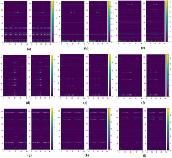
Figure 7. Feature spectra of real and reconstructed features from Task 1 data after the model has learned Task 1 (first column), Task 2 (second column), and Task 3 (third column). (a–c) Healthy; (d–f) inner faults; (g–i) outer faults.

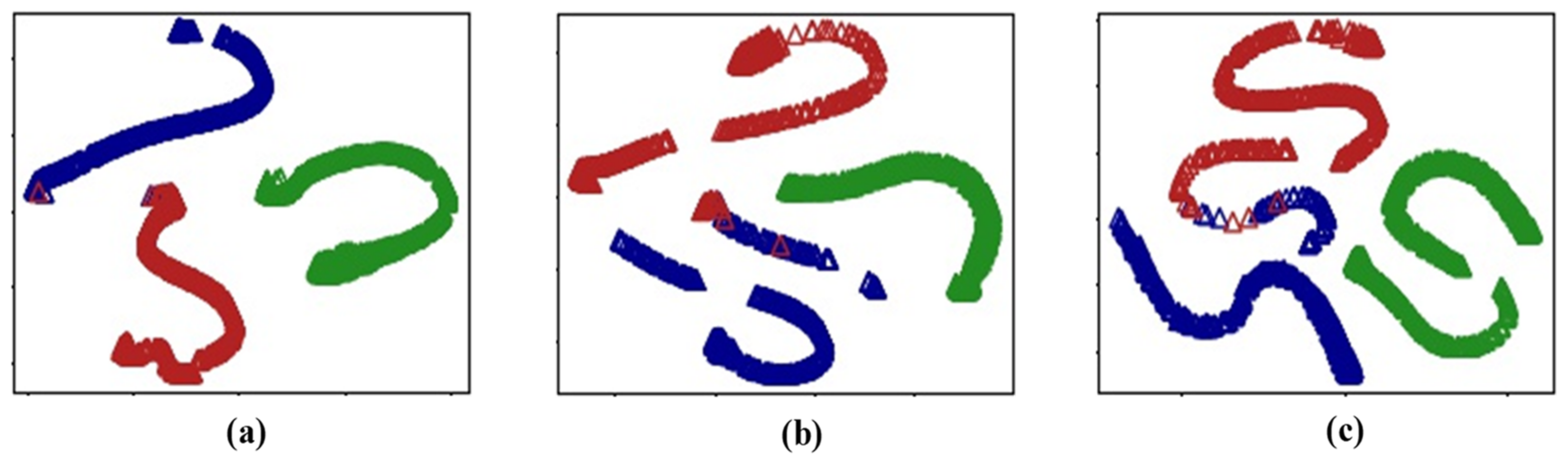
We used t-distributed stochastic neighbor embedding (t-SNE) dimensionality reduction to show the distributions of reconstructed and real features during training. Taking Task 1 as an example, the distributions at each stage are shown in Figure 8, where the subscript $i$ denotes the distribution comparison after the model completely learns Task $i$. In each subplot, the left panel shows the distribution of real features and the right panel shows the distribution of reconstructed features; the distributions are very similar. The same results were obtained for other tasks (Figure 8). The reconstructed features are reliable and representative of the historical data.

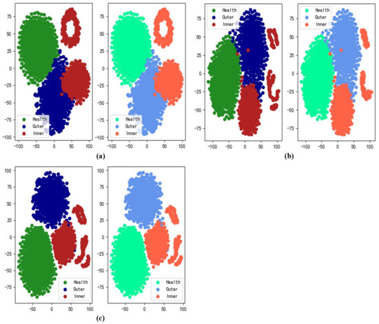
Figure 8. Distributions of reconstructed and real features from Task 1 data: (a) comparison 1; (b) comparison 2; (c) comparison 3.

4.4.2. Visualization of Training

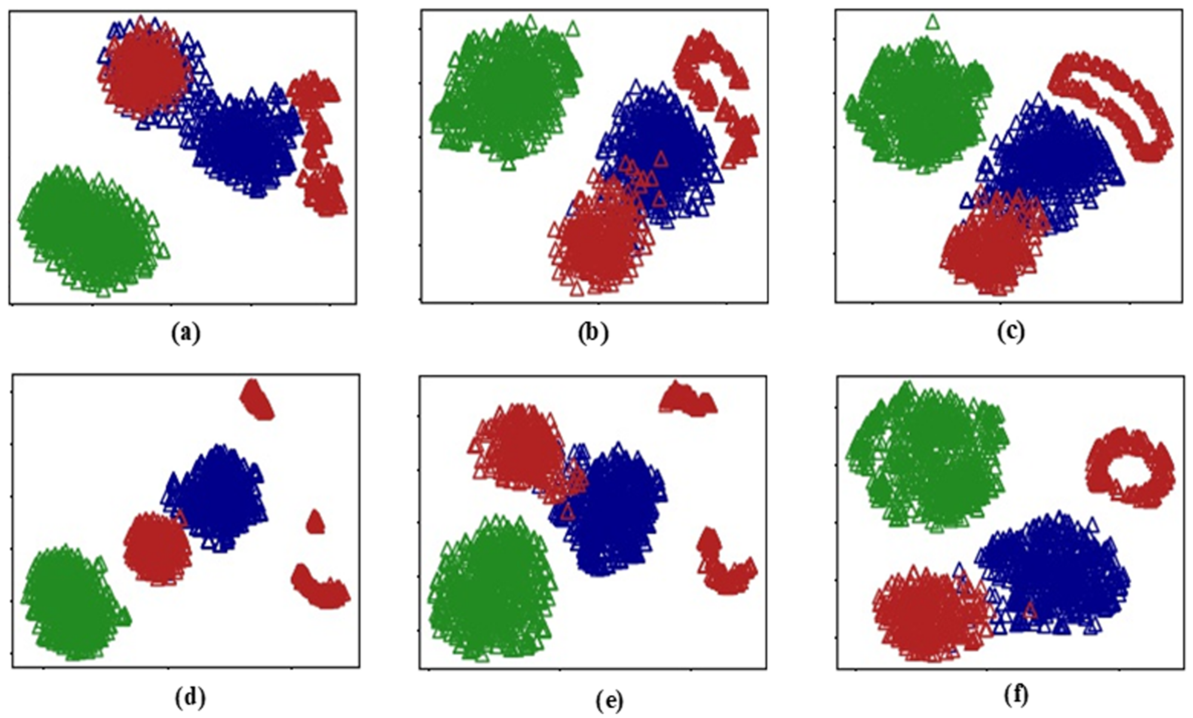
The distributions of task data are shown in Figure 9; the green points are signals from healthy bearings and the blue and red points are signals from inner and outer race faults, respectively. The Task 3 data are more similar to the Task 1 than the Task 2 data, indicating that our method reduces catastrophic forgetting after the Task 3 data have been learned during the continuous process.

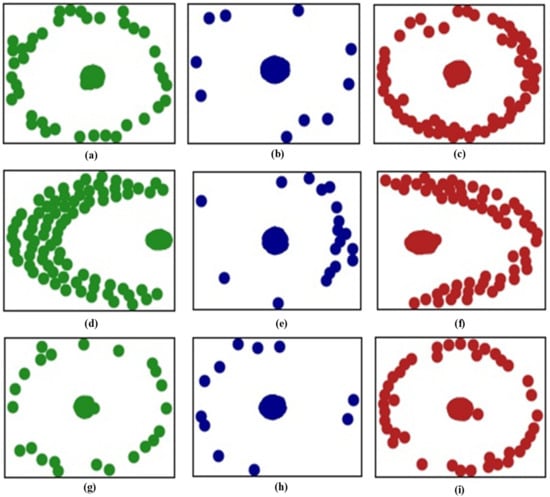
Figure 9. Distributions of task data: (a) healthy data of Task 1, (b) inner fault data of Task 1, (c) outer fault data of Task 1, (d) healthy data of Task 2, (e) inner fault data of Task 2, (f) outer fault data of Task 2, (g) healthy data of Task 3, (h) inner fault data of Task 3, and (i) outer fault data of Task 3.

To emphasize the incremental nature of learning from vibration signal features, the output results of the main modules were visualized. The Task 1 output data of the first five 1D IR-A modules (at different stages) are shown in Figure 10. In the first two columns, the change is negligible. The residuals of several 1D IR-A modules are near zero; the model degenerates into a shallow neural network because the learned data are simple. However, in the third column, comparison of (c) and (f) shows that the residual learned by the second 1D IR-A module is no longer near zero when handling complicated data, and the shortcut enhances generalizability.

Figure 10. Task 1 outputs of the first five 1D IR-A modules after the model has learned Task 1 (first column), Task 2 (second column), and Task 3 (third column) data: (a–c) 1D IR-A module 1; (d–f) 1D IR-A module 2; (g–i) 1D IR-A module 3; (j–l) 1D IR-A module 4; (m–o) 1D IR-A module 5.

As shown in Figure 11, the 1D IR-B module outputs indicate that the model can distinguish all healthy signals (green) from faults (blue and red). After the second 1D IR-B module, most inner and outer race defects are distinguished. Figure 12 shows the classification results where the outputs are visualized. Almost all of the signals from the three classes are distinguished. As the model learns new task data, there is some overlap between inner and outer race faults, which reflects mild forgetting.

Figure 11. Outputs of the first five 1D IR-B modules for Task 1 data after the model learned Task 1 (first column), Task 2 (second column), and Task 3 (third column) data: (a–c) 1D IR-B module 1; (d–f) 1D IR-B module 2.

Figure 12. Outputs of the model for Task 1 data, (a) after learning Task 1, (b) Task 2, and (c) Task 3.

4.4.3. Model Results

The results of 10 runs of R-REMIND, which continuously and sequentially learned the data of tasks, are shown in Table 5. In the Task 1 row, the first number is that obtained for the Task 1 test set after the model had finished learning Task 1 data, and the second and the third numbers are the results for the Task 1 test set after the model had learned the Task 2 and 3 data, respectively. When the model learns the data of Task 1, the Task 2 data are invisible; the Task 2 row thus shows only two numbers (the test results obtained using the data of Tasks 2 and 3, respectively). The Task 3 row is similar. The average Acc is 98.05% and the average BWT is −3.89%. The Test set 1 accuracy is over 99.63% when the model has learned the Task 1 data, but drops slightly when the Task 2 data are learned. However, accuracy tended to improve after the model had learned Task 3 because Tasks 1 and 3 are similar. For Task 2, a small amount of catastrophic forgetfulness is apparent.

Table 5. Classification results of R-REMIND (%).

Object	Experiment Number										Average
	1	2	3	4	5	6	7	8	9	10
Task 1	99.88	99.63	99.75	99.88	99.94	99.81	99.81	99.81	99.63	99.88	99.8
	98	97	97	97.81	96	95.19	94.44	97.69	96.56	98.06	96.78
	96.75	99.25	99.75	99.75	99.31	99.63	99.75	98.88	99.06	99.5	99.16
Task 2	100	99.88	100	99.94	99.88	99.94	99.63	99.81	99.94	99.81	99.88
	91.38	95.56	93.94	95.31	98.5	89.38	88.75	92.13	87.63	94.75	92.73
Task 3	99.94	99.94	99.94	99.88	99.69	100	99.94	100	100	99.94	99.93
ACC	97.66	98.54	98.4	98.76	98.89	97.33	97.05	98.05	97.14	98.66	98.05
BWT	−5.88	−2.35	−3.03	−2.38	−1.01	−5.37	−5.47	−4.31	−6.44	−2.72	−3.89

4.4.4. Results

To optimize bearing diagnosis, we used several models for comparison. We also removed R-REMIND modules in a stepwise manner to verify the effectiveness of each component. The results are shown in Table 6. Models 1 and 2 have different feature extraction networks. Model 1 uses a common CNN structure with three convolutional layers and two maxpooling layers. The parameters are those of a common feature extraction network [33]. Feature extraction of Model 2 is based on the ResNet-18 network using 1D rather than 2D convolutional layers. Model 3 is the same as R-REMIND, except that historical learned features are directly stored and replayed, where indices derived via product quantization are not used. Models 4–7 lack various R-REMIND modules, i.e., the 1D IR-A, 1D IR-B, fully connected, and buffer modules. All experiments were repeated 10 times.

Table 6. Classification results (%).

Model	Methods	Acc	BWT
R-REMIND	R-REMIND (our model)	98.05 ± 0.70	−3.89 ± 1.84
Model 1	CNN-based feature extraction network	97.66 ± 0.77	−4.74 ± 2.01
Model 2	ResNet-based feature extraction network	96.38 ± 0.72	−6.82 ± 2.21
Model 3	Feature-based buffer module	97.28 ± 0.81	−6.11 ± 2.07
Model 4	Without the 1D IR-A module	97.29 ± 0.80	−5.09 ± 2.39
Model 5	Without the 1D IR-B module	97.33 ± 0.68	−5.80 ± 1.95
Model 6	Without the fully connected module	96.69 ± 0.60	−7.46 ± 1.77
Model 7	Without the buffer module	97.25 ± 0.49	−6.20 ± 0.96

Table 6 shows that R-REMIND had the highest average accuracy (98.05%) and best BWT (–3.89%). Compared to Models 1 and 2, the combination of the 1D IR-A and 1D IR-B modules improved feature extraction from 1D bearing vibrational data. R-REMIND and Model 1 are both better than Model 2, indicating that a convolutional layer with a large kernel effectively extracts raw bearing data. As the parameters of the feature network are constantly updated, Model 3 may have cached more outdated features than R-REMIND. Furthermore, if features are stored as floating point numbers, the memory requirement is much larger than that of the indices. The Acc and BWT values of the remaining ablation models (Models 4–7) are also inferior to those of R-REMIND, emphasizing the necessity of the effectiveness of all R-REMIND components.

5. Conclusions

This study introduced R-REMIND, a novel incremental learning model that diagnoses bearing faults. The model includes feature extraction and classification networks, and a buffer module. The network is trained using both new and reconstructed (from the buffer) data, to reduce performance degradation during the recognition of old task data. The performance of our R-REMIND model was verified using a dataset from Paderborn University. Acc and BWT were used to measure performance. R-REMIND provided the best Acc and BWT (98.05 and −3.89%, respectively).

In the future, we will combine our method with other incremental learning schemes to further alleviate catastrophic forgetting. We will aim to improve the feature extraction and classification networks to include class incremental learning, and we will add an anomaly detection algorithm for online bearing monitoring.

References

- Shahriar, M.R.; Borghesani, P.; Tan, A.C.C. Electrical signature analysis-based detection of external bearing faults in electromechanical drivetrains. IEEE Trans. Ind. Electron. 2018, 65, 5941–5950. [Google Scholar] [CrossRef]
- Wang, Y.; Yang, M.; Li, Y.; Xu, Z.; Wang, J.; Fang, X. A multi-input and multi-task convolutional neural network for fault diagnosis based on bearing vibration signal. IEEE Sens. J. 2021, 21, 10946–10956. [Google Scholar] [CrossRef]
- Kudelina, K.; Baraškova, T.; Shirokova, V.; Vaimann, T.; Rassõlkin, A. Fault detecting accuracy of mechanical damages in rolling bearings. Machines 2022, 10, 86. [Google Scholar] [CrossRef]
- Yuan, H.; Wu, N.; Chen, X.; Wang, Y. Fault diagnosis of rolling bearing based on shift invariant sparse feature and optimized support vector machine. Machines 2021, 9, 98. [Google Scholar] [CrossRef]
- Nguyen, V.C.; Hoang, D.T.; Tran, X.T.; Van, M.; Kang, H.J. A bearing fault diagnosis method using multi-branch deep neural network. Machines 2021, 9, 345. [Google Scholar] [CrossRef]
- Ni, Q.; Ji, J.C.; Feng, K.; Halkon, B. A novel correntropy-based band selection method for the fault diagnosis of bearings under fault-irrelevant impulsive and cyclostationary interferences. Mech. Syst. Signal Process. 2021, 153, 107498. [Google Scholar] [CrossRef]
- Ni, Q.; Ji, J.C.; Feng, K.; Halkon, B. A fault information-guided variational mode decomposition (FIVMD) method for rolling element bearings diagnosis. Mech. Syst. Signal Process. 2022, 164, 108216. [Google Scholar] [CrossRef]
- Sabir, R.; Rosato, D.; Hartmann, S.; Guehmann, C. LSTM based bearing fault diagnosis of electrical machines using motor current signal. In Proceedings of the 2019 18th IEEE International Conference on Machine Learning and Applications (ICMLA), Boca Raton, FL, USA, 16–19 December 2019; pp. 613–618. [Google Scholar]
- Hoang, D.T.; Kang, H.J. A motor current signal-based bearing fault diagnosis using deep learning and information fusion. IEEE Trans. Instrum. Meas. 2020, 69, 3325–3333. [Google Scholar] [CrossRef]
- Elforjani, M.; Shanbr, S. Prognosis of bearing acoustic emission signals using supervised machine learning. IEEE Trans. Ind. Electron. 2018, 65, 5864–5871. [Google Scholar] [CrossRef] [Green Version]
- Liu, Z.; Wang, X.; Zhang, L. Fault diagnosis of industrial wind turbine blade bearing using acoustic emission analysis. IEEE Trans. Instrum. Meas. 2020, 69, 6630–6639. [Google Scholar] [CrossRef]
- Shao, H.; Xia, M.; Han, G.; Zhang, Y.; Wan, J. Intelligent fault diagnosis of rotor-bearing system under varying working conditions with modified transfer convolutional neural network and thermal images. IEEE Trans. Ind. Inform. 2021, 17, 3488–3496. [Google Scholar] [CrossRef]
- Wang, J.; Liang, Y.; Zheng, Y.; Gao, R.X.; Zhang, F. An integrated fault diagnosis and prognosis approach for predictive maintenance of wind turbine bearing with limited samples. Renew. Energy 2020, 145, 642–650. [Google Scholar] [CrossRef]
- Liang, T.; Wu, S.; Duan, W.; Zhang, R. Bearing fault diagnosis based on improved ensemble learning and deep belief network. J. Phys. Conf. Ser. 2018, 1074, 012154. [Google Scholar] [CrossRef]
- Jiang, H.; Li, X.; Shao, H.; Zhao, K. Intelligent fault diagnosis of rolling bearings using an improved deep recurrent neural network. Meas. Sci. Technol. 2018, 29, 065107. [Google Scholar] [CrossRef]
- Hoang, D.T.; Kang, H.J. Rolling element bearing fault diagnosis using convolutional neural network and vibration image. Cogn. Syst. Res. 2019, 53, 42–50. [Google Scholar] [CrossRef]
- Pham, M.T.; Kim, J.M.; Kim, C.H. 2D CNN-based multi-output diagnosis for compound bearing faults under variable rotational speeds. Machines 2021, 9, 199. [Google Scholar] [CrossRef]
- He, J.; Li, X.; Chen, Y.; Chen, D.; Guo, J.; Zhou, Y. Deep transfer learning method based on 1d-cnn for bearing fault diagnosis. Shock Vib. 2021, 2021, 1–16. [Google Scholar] [CrossRef]
- Han, T.; Liu, C.; Wu, L.; Sarkar, S.; Jiang, D. An adaptive spatiotemporal feature learning approach for fault diagnosis in complex systems. Mech. Syst. Signal Process. 2019, 117, 170–187. [Google Scholar] [CrossRef]
- Razavi-Far, R.; Farajzadeh-Zanjani, M.; Saif, M.; Palade, V. A hybrid ensemble scheme for diagnosing new class defects under non-stationary and class imbalance conditions. In Proceedings of the 2017 International Conference on Sensing, Diagnostics, Prognostics, and Control (SDPC), Shanghai, China, 16–18 August 2017; pp. 355–360. [Google Scholar]
- Razavi-Far, R.; Saif, M.; Palade, V.; Zio, E. Adaptive incremental ensemble of extreme learning machines for fault diagnosis in induction motors. In Proceedings of the 2017 International Joint Conference on Neural Networks (IJCNN), Anchorage, AK, USA, 14–19 May 2017; pp. 1615–1622. [Google Scholar]
- Kang, J.; Liu, Z.; Sun, W.; Zuo, M.J.; Qin, Y. A class incremental learning approach based on autoencoder without manual feature extraction for rail vehicle fault diagnosis. In Proceedings of the 2018 Prognostics and System Health Management Conference (PHM-Chongqing), Chongqing, China, 26–28 October 2018; pp. 45–49. [Google Scholar]
- Yang, Z.; Long, J.; Zi, Y.; Zhang, S.; Li, C. Incremental novelty identification from initially one-class learning to unknown abnormality classification. IEEE Trans. Ind. Electron. 2022, 69, 7394–7404. [Google Scholar] [CrossRef]
- Wang, Y.; Zeng, L.; Ding, X.; Wang, L.; Shao, Y. Incremental learning of bearing fault diagnosis via style-based generative adversarial network. In Proceedings of the 2020 International Conference on Sensing, Measurement & Data Analytics in the era of Artificial Intelligence (ICSMD), Xi’an, China, 15–17 October 2020; pp. 512–517. [Google Scholar]
- Wang, Y.; Zeng, L.; Wang, L.; Shao, Y.; Zhang, Y.; Ding, X. An efficient incremental learning of bearing fault imbalanced data set via filter styleGAN. IEEE Trans. Instrum. Meas. 2021, 70, 107498. [Google Scholar] [CrossRef]
- Li, F.; Chen, J.; He, S.; Zhou, Z. Layer regeneration network with parameter transfer and knowledge distillation for intelligent fault diagnosis of bearing using class unbalanced sample. IEEE Trans. Instrum. Meas. 2021, 70, 3522210. [Google Scholar] [CrossRef]
- Hayes, T.L.; Kafle, K.; Shrestha, R.; Acharya, M.; Kanan, C. REMIND your neural network to prevent catastrophic forgetting. In Proceedings of the 16th European Conference on Computer Vision (ECCV), Glasgow, UK, 23–28 August 2020; pp. 466–483. [Google Scholar]
- He, K.; Zhang, X.; Ren, S.; Sun, J. Deep residual learning for image recognition. In Proceedings of the 2016 IEEE Conference on Computer Vision and Pattern Recognition (CVPR), Las Vegas, NV, USA, 27–30 June 2016; pp. 770–778. [Google Scholar]
- Szegedy, C.; Ioffe, S.; Vanhoucke, V.; Alemi, A.A. Inception-v4, Inception-ResNet and the impact of residual connections on learning. In Proceedings of the 31st AAAI Conference on Artificial Intelligence(AAAI), San Francisco, CA, USA, 4–9 February 2017; pp. 4278–4284. [Google Scholar]
- Jégou, H.; Douze, M.; Schmid, C. Product quantization for nearest neighbor search. IEEE Trans. Pattern Anal. Mach. Intell. 2011, 33, 117–128. [Google Scholar] [CrossRef] [Green Version]
- Simonyan, K.; Zisserman, A. Very Deep Convolutional Networks for Large-Scale Image Recognition. Available online: https://arxiv.org/abs/1409.1556 (accessed on 3 April 2022).
- Lessmeier, C.; Kimotho, J.K.; Zimmer, D.; Sextro, W. Condition monitoring of bearing damage in electromechanical drive systems by using motor current signals of electric motors: A benchmark data set for data-driven classification. In Proceedings of the European Conference of the Prognostics and Health Management Society(PHME16), Bilbao, Spain, 5–8 July 2016; pp. 5–8. [Google Scholar]
- Song, Y.; Li, Y.; Jia, L.; Qiu, M. Retraining strategy-based domain adaption network for intelligent fault diagnosis. IEEE Trans. Ind. Inform. 2020, 16, 6163–6171. [Google Scholar] [CrossRef]
Publisher’s Note: MDPI stays neutral with regard to jurisdictional claims in published maps and institutional affiliations. |
© 2022 by the authors. Licensee MDPI, Basel, Switzerland. This article is an open access article distributed under the terms and conditions of the Creative Commons Attribution (CC BY) license (https://creativecommons.org/licenses/by/4.0/).