Feature-Based and Process-Based Manufacturing Cost Estimation

Abstract

The demand for mass custom parts is increasing, estimating the cost of parts to a high degree of efficiency is a matter of great concern to most manufacturing companies. Under the premise of machining operations, cost estimation based on features and processes yields high estimation accuracy, but it necessitates accurately identifying a part’s machining features and establishing the relationship between the feature and the cost. Accordingly, a feature recognition method based on syntactic pattern recognition is proposed herein. The proposed method provides a more precise feature definition and easily describes complex features using constraints. To establish the relationships between geometric features, processing modes, and cost, this study proposes a method of describing the features and the processing mode using feature quantities and adopts deep learning technology to establish the relationship between feature quantities and cost. By comparing a back propagation (BP) network and a convolutional neural network (CNN) it can be concluded that a CNN using the “RMSProp” optimizer exhibits higher accuracy.

1. Introduction

With the formation of the global economic market and the rapid development of the internet, various new technologies have continued to emerge, and competition in the field of machinery manufacturing has become increasingly fierce. This is mainly manifested in the acceleration of product research and development, shortening of product life cycles, dynamic changes and diversifications of customer demand, continuous innovation of complex and new technologies, and frequent renewal of products. To adapt to the current competitive market environment, parts manufacturers must save time, starting from cost estimation until the completion of the entire process of parts manufacturing, and strive to produce products that meet the needs of customers in the shortest possible time. However, most of the existing methods for estimating costs of parts consider only the geometric features of the parts or have low accuracy, which leads to errors or even complete mistakes in the cost estimation results. In this study, we aimed to introduce feature quantities into the machining process to describe the features of a part and achieve efficient and accurate cost estimation of parts. The method first identified features based on syntactic patterns and described complex features through the feature constraints of the part, thus allowing for more accurate feature definition and more efficient identification. Thereafter, feature quantities were established to describe features and machining patterns to determine the relationship among geometric features, machining patterns, and the cost of a part.

2. Related work

2.1. Analysis Estimation Methods

Analysis estimation methods aim to obtain cost statistics information according to product structure information and cost information and to estimate cost through a parameter-fitting relationship. The mature algorithms in this space are as follows. ① A learning curve estimation method assumes that owing to continuous repetition of fixed mode work in a certain period of time, the work efficiency will increase at a certain rate, the descent curve shows the relationship between the number of tasks and the completion time [1]. The neural network strategy is based on the premise that a regression relationship between cost and influencing factors can be established. A large number of data training exercises are used to improve the robustness of the network and compute cost estimates [2,3]. ② Activity-based costing [4] is based on the basic principle of ‘products consume activities, activities consume resources’. It confirms and measures all the activities where enterprises consume resources, records the cost of the consumed resources into various activities, and then estimates the product cost. Activity-based costing has high accuracy but must be conducted after the completion of product design. ③ The multi-attribute fuzzy method analyses the cost influence factors in product design stage, determines the upper and lower limits of cost drivers and weight coefficients, and conducts the cost estimation according to a fuzzy multi-attribute effect theory method of product influence factors [5,6]. ④ A similarity estimation method [7,8] estimates the cost of products using similarity relationships between the products; the key of this method is to calculate the similarity of products. Analysis estimation methods do not need to analyze every link of a commodity cost in detail. Owing to the small amount of estimation work, it can obtain a relation for cost estimation. Therefore, it is commonly utilized in the early phases of product development, but its accuracy is not high.

2.2. Feature-Based and Process-Based Estimation Method

An estimation method based on features and processes considers the cost estimation process as a process of adding features regarding cost-influencing factors. The accuracy of the estimation result is higher, and the error is smaller as this method directly addresses the “drivers” causing the cost. Methods of this type require complete knowledge of the product attributes and require a thorough understanding of the factors affecting the cost of parts in the design and manufacturing processes. Based on this information, a mathematical expression is used to estimate the cost of parts.

Federico Campi et al. [9] proposed an analytical model to estimate the cost of axisymmetric components produced with open die-forging. The part’s geometrical features (e.g., dimensions, shape, and material as well as tolerances) are input into the model. According to the case studies, the cost models provide accurate results regarding cost breakdown. Grund et al. [10] devised a statistical technique for calculating unit costs of components (such as a part’s construction height or capacity consumption) and converted these approaches to a generic model in their work. Lin and Shaw [11] established a topology for the relationships between features by linking general dimensional parameters and detailed features of specifications (e.g., designs and cost information) to estimate the main cost items of a ship. The features were extracted and transformed into a quantifiable structure. The errors of the estimated total costs were less than 7%.

Table 1 shows the comparison of different cost estimation methods.

Table 1. Comparison of various estimation methods.

Method Type	Method Name	Estimation Accuracy	Method Difficulty	Product Information Required
Analysis estimation methods [1,2,3,4,5,6,7,8]	Learning curve estimation method [1]	Low	General difficulties	They need more parts manufacturing information
	Neural network estimation method [2]
	Activity based costing estimation method [3,4]
	Multi-attribute fuzzy method [5,6]
	Similarity estimation method [7,8]
Feature-based and process-based estimation method	Machining feature recognition [9,10,11]	High	Difficult	It needs a large amount of information, including part design and manufacturing information

2.3. Manufacturing Feature Recognition

Manufacturing feature recognition has evolved over the past half-century. It has several approaches. Generally, the methods can be divided into two categories: those based on boundary matching and those based on stereo decomposition.

2.3.1. Logic Rules and Expert Systems

This approach defines manufacturing parts’ features as a series of trigger rules (IF A₁, A₂, A₃, …, A_n, THEN C), and identifies them as soon as the conditions $({\mathrm{A}}_1,{\mathrm{A}}_2,{\mathrm{A}}_3,\dots ,{\mathrm{A}}_{\mathrm{n}})$ are met [12,13]. The key to this approach is describing the manufacturing feature by a series of (IF, THEN) statements, and ensuring that all descriptions are unique. For complex and diverse features, as the number of definitions increases, the descriptions become clumsier and more complex, and the systems require more calculations and matching. Thus, this method works well for identifying simple features, but there are recognition errors in cases of complex and intersecting features.

2.3.2. Graph-Based Approach

In 1987, Joshi [14,15,16] proposed this approach to recognize features from 3D model parts based on the attribute adjacency graph. An attributed adjacency graph is formed by transforming model parts topological information into nodes of faces and arcs of edges. While this method can recognize independent features very accurately, on negative polyhedra it fails to do so. The multi-attributed adjacency graphs (MAAG) were proposed by Venuvinod and Wong [17] as a way to make the attributes of the adjacency graph more accurate, especially those of faces. For example, if an angle is formed between two neighboring faces, then a new attribute value is assigned. Dong et al. [18] described MAAG as ‘less expert system and more algorithmic’ for form pattern recognition. However, the disadvantage of MAAG makes it impossible to describe the case of feature-intersection.

2.3.3. Convex Hull Volumetric Decomposition

A feature recognition method based on convex hull volumetric decomposition was first implemented by Woo [19]. By defining the different volumes of the part model and convex hull as a volume interleaved sum, the model is represented as a model decomposition tree with a convex body. In this tree, a convex element is a leaf. In the convex decomposition method, the first leaf determines whether each leaf itself corresponds to a specific feature; if it does not, then the leaf uses the related combination operation to combine it with other leaf nodes to make it correspond to a feature. However, this method cannot guarantee that the decomposition of non-convex objects will always converge. Kim [20] improved this alternating sum of volumes using the partitioning decomposition method and effectively solved the problem of the non-convergence of the volume decomposition in the Woo method.

2.3.4. Cell-Based Decomposition Approach

In the cell-based decomposition approach, the volume of the part removed from the blank is first identified and then the volume is decomposed into unit bodies. The largest unit body that can be cut in a machining path is obtained by combining the units with the same plane or those that are coplanar. This method can effectively identify and provide multiple interpretations of intersection features [21,22]. However, there are two outstanding problems. First, the algorithm efficiency is very low because of the need for numerous intersection calculations and the numerous composite elements generated. Second, there are too many generated feature interpretations, with a slightly complex part having hundreds of them. Thus, it is unrealistic to generate and process too many feature interpretations.

2.3.5. Hint-Based Approach

In this approach, the total processed body of the parts is decomposed into the smallest processed body, and the features are manufactured by reorganizing the parts with the characteristic trace remaining in the smallest processed body [23,24,25]. The feature trace is the retained information in the part models. When features intersect, the complete boundary information is lost, but if it includes features, there will be a trace in the model, including specific design features and processing information. This approach is advantageous in feature-intersection problems, particularly for adding virtual chains to construct complete processing faces. However, for complex features, there are cases where the recognition rate is low, and depending on the feature type, it is difficult to add new features.

2.3.6. Convolutional Neural Network (CNN) Recognition Approach

As deep-learning technology develops rapidly, machine learning is studied to recognize the features of various types of parts [26,27,28,29]. Zhang [30] proposed a three-dimensional (3D) CNN to solve this problem using individual features on a cube block and generating several features of different sizes to obtain a large amount of feature data, trained and classified. Then, the features were decomposed based on the watershed approach. Finally, feature recognition was achieved, and good results were obtained. Yang Shi [31,32] investigated a novel approach to feature description as a way to solve the feature interaction problem. A descriptor called heat kernel signature (HKS) was input into a two-dimensional (2D) CNN, and the the final results showed that this feature representation could better solve the boundary losses problem caused by feature interactions. Thus, the performance of interacting feature recognition was improved.

2.3.7. Ray-Distance Feature-Recognition Approach

Rakesh used the “excited ray” concept to set different features based on the information for different rays excited by the different surfaces of parts [33]. First, the virtual plane is defined to detect and capture the ray excited from the solid surface points to the virtual plane, and then the ray distances from the surface points to the virtual plane are calculated to define and identify different features.

2.3.8. Cavity Volume Method

The principle of this method is to define the volume of the material that needs to be removed in the process of machining [34]. Develop logical rules for features and when a feature meets the corresponding logical requirements, then it will be recognized. In order to identify the feature volumes that can be machined, these logic rules are formalized into “feature rules.” In formal programs, a feature is defined as a production rule when the condition is A_n and the part feature is C. For example, (IF A₁, A₂, A₃, …, A_n, THEN C) would be the production rule. The difference between this method and logic rules is that the feature system only deals with those swept volumes for which the extent of the sweep is known, such as holes, slots, and pockets of arbitrary complexity.

When designing a part, it is not only necessary to consider how it is machined and its use, but also to analyze the mechanical properties of the part, which makes the structural form of parts complex [35]. The 3D model of a part only contains limited information about its geometry and topology, these factors bring great challenges to the traditional method of feature recognition based on geometry and topology—as shown in Table 2—which are mainly manifested in the following two aspects: 1. The recognition is not accurate. Using the traditional method makes it difficult to describe the part model using limited information, and the parts geometry and machining features are difficult to reflect accurately; 2. A large amount of computation is required. Because of the limited known information in the traditional methods, calculations need to be repeated to obtain more information. In this newly emerging field, deep learning allows a large amount of data to be used to automatically understand special mapping relationships and advanced data features. In summary, the application of deep learning-based classification models is effective in reducing the difficulty of part feature recognition and improving its accuracy.

Table 2. Comparison of part feature recognition methods.

Method	Principle	Difficulty	Limitation
Graph-based approach	AAG	Higher	Large amount of calculation and inaccurate identification of intersecting features
Hint-based approach	Trace recombination		Complex features are difficult to recognize, and the recognition rate is low
Logic rules and expert systems approach	Defining features and triggering rules	Average	Complex features are difficult to recognize
Convex hull volumetric decomposition approach	Split parts		Low efficiency and large amount of calculation
Cell-based decomposition
Cavity volume method	Defining features		Complex features are difficult to recognize
CNN recognition approach	Feature classification		Difficult to locate features
Ray-distance feature-recognition approach	Excitation ray	Lower	High error rate

This section has provided an overview of cost estimation and feature recognition of parts. As discussed, cost estimation based on manufacturing features and processes has higher accuracy but requires accurately identifying the manufacturing features of parts and establishing relationships between features and cost. There are some problems in manufacturing feature recognition, such as a slow recognition speed, large amounts of calculation, and inaccurate recognition. Therefore, in Section 3, a method for recognizing features using syntactic patterns is presented. Section 4 elaborates on the innovative concept of this study, i.e., describing manufacturing features through feature quantities. In Section 5, the feature-cost relationship is obtained by applying CNN networks and BP networks.

3. Syntactic Pattern-Recognition Approach

3.1. Syntactic Pattern Recognition

With the increasing popularity of computers and calculators, pattern recognition has undergone significant developments in theory and application. The methods of pattern recognition are classified into four categories: intelligent patterns, fuzzy mode methods, statistical, and syntactic [36]. A syntactic pattern-recognition approach [37,38] involves combining identified patterns (samples or graphics) into a sentence according to their structure. Then, syntactic pattern recognition is employed to determine which category they belong to. When the patterns are complex, there can be numerous features, or the number of schema classes can be large such that simple pattern classification is not capable of identifying a mechanical machining feature. In such cases, a simple sub-pattern is needed to form a hierarchy for describing the complex pattern. Assuming that this sub-pattern is divided into primitives, then complex patterns will be recognized through identification of the primitives within it.

3.2. Feature Constraints and Definitions

Parts having specific functions are expressed by a particular configuration represented by their geometric features, and the modelling of a part contains geometric features constructed by geometric information through topological relationship. For part manufacturing, the geometric information is the core expression characteristic and includes geometric elements such as vertices, edges, and faces. These geometric elements are coordinates of the vertices, normals, and types of the edges and faces.

A 3D model of parts consists of feature entities, which are interrelated and constrained to meet the needs of different life cycles [39]. In addition, a constraint is also used to model the features of parts, thereby forming feature constraints [40]. These constraints are the core parts of the model for describing the behavior of the specific features and attributes. The geometric topological relationship and constraint relationship in part features are represented by the spatial position relationships, including parallel, coaxial, vertical, coplanar, distance, intersect, tangency, projection, symmetrical and deviate.

The syntax feature recognition constraint relationship is defined as follows:

Let the boundary of a solid consist of a set of faces $F=\left\{f_i\right\}, i=1 \dots n$, where n equals the number of faces constituting the solid. We denote a face, f_i, which is under consideration, as the parent face. Let be constrained by loops l_i1, …, l_ij. Let e_ijk denote the k^lh edge of the j^lh loop of the i^lh face and let $E_{ij}=\left\{e_{ijk}\right\}$ denote the set of all edges of loop l_ij of face f_i. In the B-rep structure, an edge can be associated with two and only two faces. Thus for every edge, e_ijk, of a parent face, f_i, one can identify another face, f_m, $m\ne i$ and $0<m\le n$, of the same solid, which is termed as the adjacent face, such that, $e_{ijk}=f_i\cap f_m$. Thus, for a given parent face, one can identify an adjacent face through every edge of every loop of the face. We denote the adjacent face, f_i, through edge, e_ijk, as

$$f_m=adj\left(f_i,e_{ijk}\right)$$

(1)

For a given parent face, $f_i$, let $\widehat{E}=\left\{e_{ijk},e_{ijk+1},\dots ,e_{ijk+l}\right\}$ be an identified sequence of finite, consecutive edges such that the corresponding adjacent faces,

$$\widehat{F}=\left\{adj\left(f_i,e_{ijk},adj\left(f_i,e_{ijk+1}\right),\dots ,adj\left(f_i,e_{ijk+l}\right)\right)\right\}$$

(2)

together constitute a geometric form feature.

(1)

Joint-Edge (f₁, f₂, angle), where f_i and angle are the primitives belonging to faces and the non-solid angles between faces, respectively;

(2)

Parallel (x₁, x₂), where x₁ and x₂ are the primitives;

(3)

Vertical (x₁, x₂), where x₁ and x₂ are the primitives;

(4)

Coplanar (x₁, x₂), where x₁ and x₂ are the primitives;

(5)

Intersect (x₁, x₂), where x₁ and x₂ are the primitives;

(6)

Projection (x₁, x₂, d), where x₁ and d are the primitives and the direction of its projection respectively;

(7)

Symmetrical (x₁, x₂, s), where s is the axis of symmetry of the primitives x₁ and x₂;

(8)

Deviate (x₁, x₂, v, m), where m is the offset from primitive x₁ to x₂ and v is the direction of m;

(9)

Distance (x₁, x₂), where x₁ and x₂ are the primitives;

(10)

Coaxial (x₁, x₂), where x₁ and x₂ are the primitives.

3.3. Clue Hints and Search Directions

In syntactic pattern recognition, a parts manufacturing feature is identified by Joint-Edge; thus, the feature faces are connected in series, and the features are confirmed using the constraint relationships. In this approach, if the first face is determined for a feature in the entities, the features are easy to identify. When searching for the first face, all faces must be traversed. To improve the recognition efficiency, a definition datum is added, and provides a clue regarding the first face.

Considering the variable faces of the parts (such as the top and bottom faces of the features) and the types and numbers of edges and faces, the inner and outer loops are uncertain. Therefore, the side faces are selected as the defining reference faces. As the types of side faces, concave edges of the outer loops, convex edges, and number of trimming edges are regular, they are defined as clues.

In addition, the Joint-Edge is defined by adjacent faces; however, for parts with additional faces, there are more neighboring faces. Thus, all these faces must be traversed. A vector anticlockwise angle of the two sides is provided in the definition to accurately describe the position of the next face.

$$\sin (\overrightarrow{a},\overrightarrow{b})=\frac{\overrightarrow{a}\times \overrightarrow{b}}{\mathrm{norm}(\overrightarrow{a})\mathrm{norm}(\overrightarrow{b})}$$

(3)

$$\cos (\overrightarrow{a},\overrightarrow{b})=\frac{\overrightarrow{a}\cdot \overrightarrow{b}}{\mathrm{norm}(\overrightarrow{a})\mathrm{norm}(\overrightarrow{b})}$$

(4)

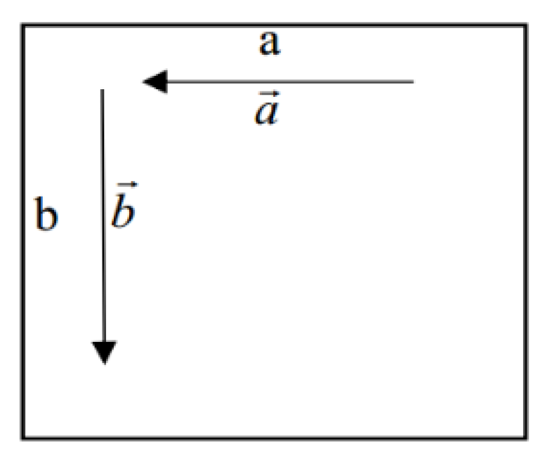
$(\overrightarrow{a},\overrightarrow{b})$ is the angle of vector $\overrightarrow{a}$, rotated anticlockwise to the vector $\overrightarrow{b}$.

$$\tan (\overrightarrow{a},\overrightarrow{b})=\frac{\overrightarrow{a}\times \overrightarrow{b}}{\overrightarrow{a}\cdot \overrightarrow{b}}$$

(5)

The anticlockwise angle of $\overrightarrow{a}$ $\overrightarrow{b}$ is expressed as

$$\mathrm{cont} (\overrightarrow{a}, \overrightarrow{b})=\pi +\mathrm{atan} (\tan (\overrightarrow{a}, \overrightarrow{b}\left)\right)$$

(6)

As shown in Figure 1, assuming that the vector of side a ($\overrightarrow{a}$) is known, $\overrightarrow{b}=\mathrm{cont}(a,\pi /2)$. Some faces are defined by calculating the anticlockwise rotation angle of the vector of the edge.

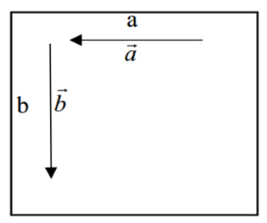
Figure 1. Edge vector.

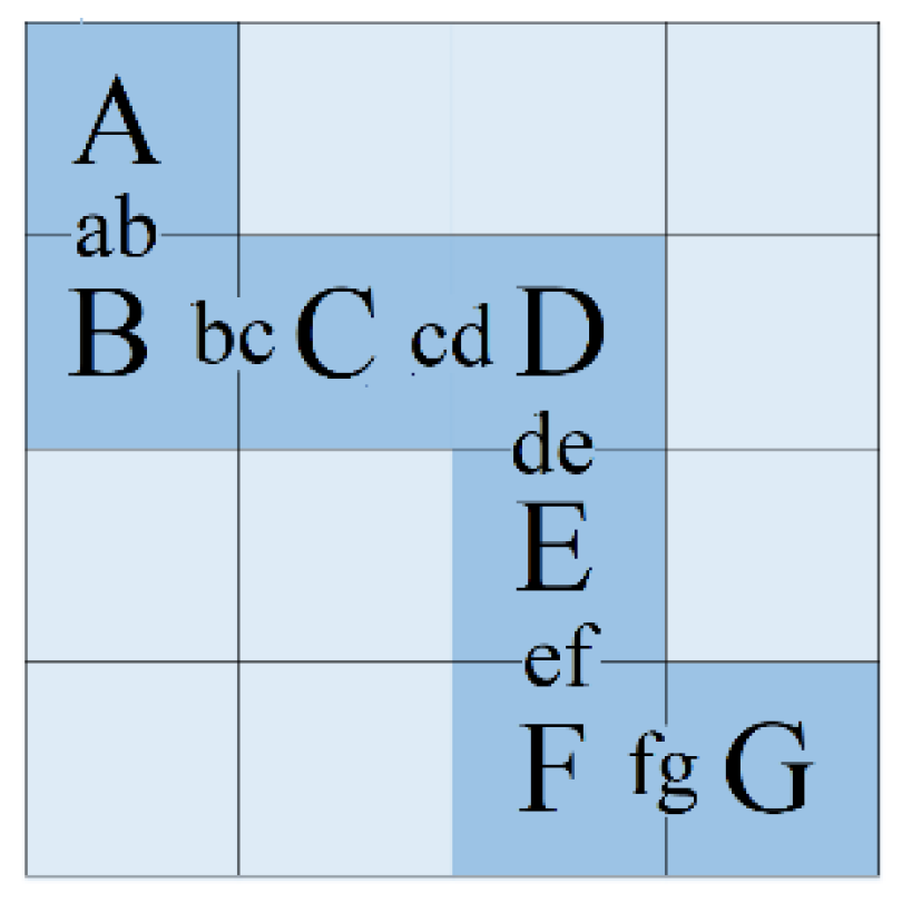
As illustrated in Figure 2, assuming that the normal vectors of the 16 faces point outward, the red face is selected according to the anticlockwise angle between the two sides. If the intersection line ab of the AB faces is known, the CDEFG faces are determined using the anticlockwise angle.

fg = cont(cont(cont(cont(cont(ab, 1.5π), π), 1.5π), π), 1.5π)

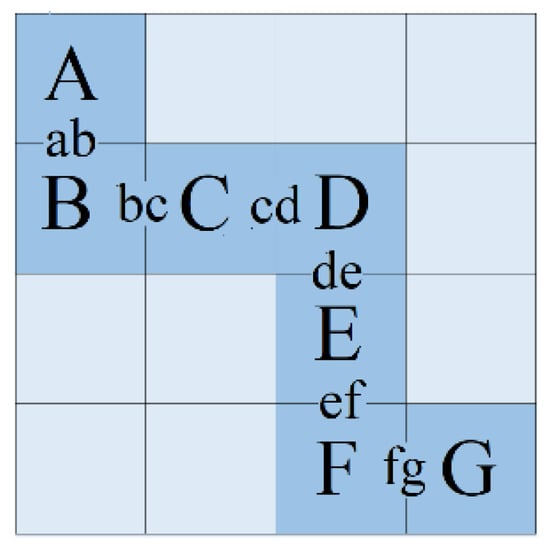
Figure 2. Selecting specific faces.

3.4. Feature Recognition of T-Groove

3.4.1. Selecting Definition Datum

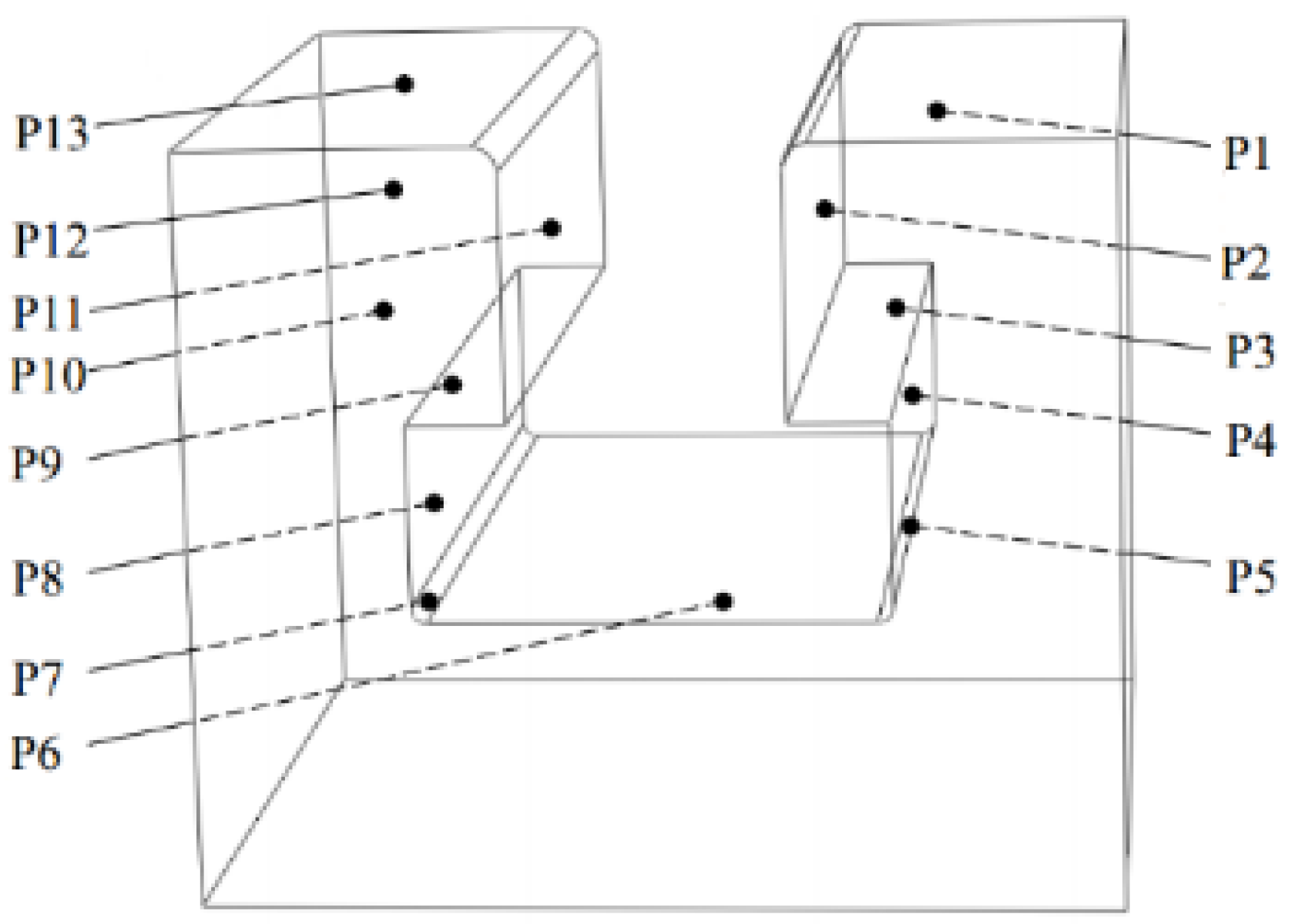
Figure 3 shows a typical part manufacturing feature: a T-Groove. The P11 face is selected as the definition datum, and the clue indicates the following condition: the face has three convex edges, and one trim.

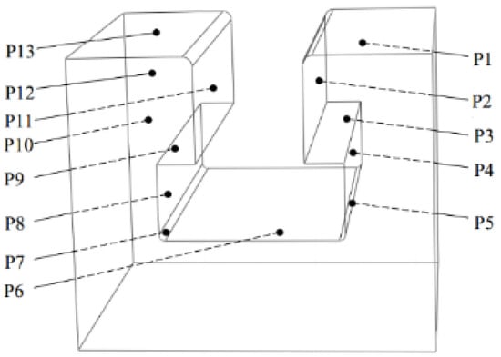
Figure 3. T-Groove( P1-P13 are the correlation surfaces of the features).

3.4.2. Syntactic definition of T-Groove feature

The T-Groove feature faces include P2–P9 and P11. The defining order of the faces is P11→P9→P8→P7→P6→P5→P4→P3→P2. The T-Groove syntax pattern is defined as follows: Joint-Edge (Joint-Edge (Joint-Edge (Joint-Edge (Joint-Edge (Joint-Edge (Joint-Edge (Joint-Edge (Joint-Edge (P11, P9,1.5π)P9(π), P8,0.5π)P8(π),P7, π)P7(π), P6,π)P6(π), P5,π)P5(π), P4,π)P4(π), P3,0.5π)P3(π), P2,1.5π)P2(π) ∩Parallel(P11,P8) ∩Parallel(P11,P4) ∩Parallel(P11,P2) ∩Parallel(P9,P3) ∩Coplanar(P7,P5).

4. Feature Recognition and Feature Quantities Calculation

4.1. Feature Quantity Calculation

Features and machining characteristics affect the cost. Feature quantization is a method used to establish a cost-feature regression relationship in this paper: the manufacturing characteristics and geometric features of parts are converted into quantities. There are different types of geometric features, and therefore the corresponding feature quantities, which are shown in Table 3, are calculated based on the type of feature.

Table 3. Feature quantities of each geometric features.

Geometric Features	Characteristic Quantities	Common Characteristic Quantities
Through hole	Diameter, Face area, Hole depth	Envelope volume Envelope center of gravity Position coefficient
Non-through hole	Diameter, Face area, Hole depth
Through trough	Groove area and depth
Eccentric shaft	Diameter, Length, Eccentricity, Axis, Top and bottom area
Non-through trough	Groove area and depth
Cylindrical shaft	Diameter, Length, Eccentricity, Axis, Top and bottom area

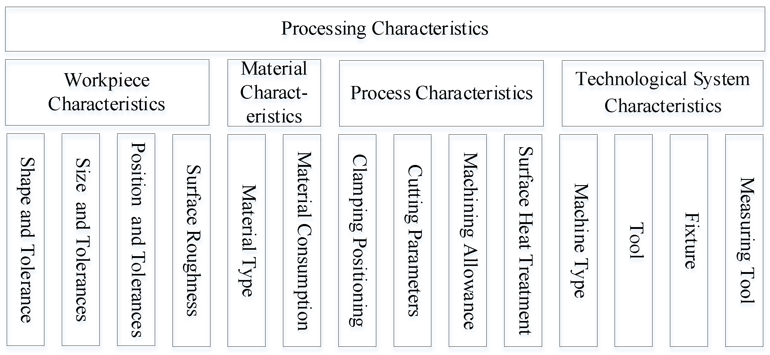
The cost of parts depends on the manufacturing cost, where the most important factor is the processing. The difficulty of machining parts is closely related to their geometric features and material characteristics, as well as the machining process, as shown in Figure 4. The cost of a part depends primarily on the manufacturing characteristics, including the geometric, material, process, and machine tool features.

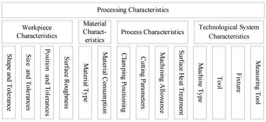
Figure 4. Machining characteristics of parts.

For the manufacturing feature description of the parts, the corresponding feature quantities are described in the form of assignments, as shown in Table 4. For a 2D CNN, these feature quantities are only a scalar representation of the factors influencing the cost.

Table 4. Quantities corresponding to each machining feature.

Processing Characteristic	Feature Quantities	Value
Locating positioning	Two pins and one surface	0
	Two surfaces and one pin	1
	V-block and diamond pin	2
Surface heat treatment	Hard facing	0
	Chemical heat treatment	1
	Contact resistance heating quenching	2
	Electrolytic heating quenching	3
	Electron beam heat treatment	4
	Laser heat treatment	5
Machine type	Conventional machine tool	0
	High-precision machine tool	1
	Computer numerical control machine tool	2
Fixture	Universal fixture	0
	Dedicated fixture	1
	Flexible fixture	2
	Combination fixture	3
Tools	High-speed tool	0
	Cemented carbide cutter	1
	Ceramic tool	2
	Cubic boron nitride cutting tool	3
	Diamond cutting tools	4
Measuring tool	Universal measuring tool	0
	Special measuring tool	1
	Standard gauge	2

4.2. Feature-Recognition Process

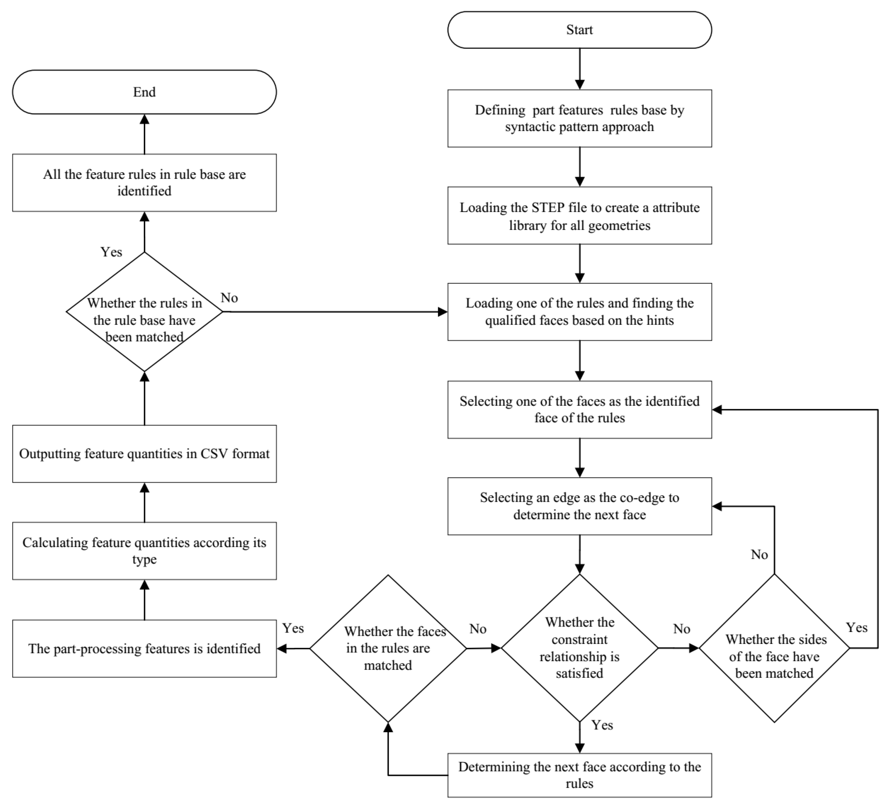
Figure 5 illustrates the machining features recognition process: ① used syntactic patterns for defining geometrical features in order to form the corresponding rule base for describing those features. The mechanical parts contained several common machining features, such as knife-withdrawal-groove, dovetail-groove, T-Groove, and keyway; ② the STEP file was loaded. All geometric information, such as lists of vertices, lines, and polygons was obtained and a library of properties for each face was created according to the constraint rules. Matching was processed as follows: first, all satisfying faces that match were selected by the cue prompt and one face from the satisfying faces was identified as the primary face recognizable by the rule. Then, a common edge was selected from the primary face to identify the neighboring face of the primary face, and that neighboring face was examined against the constraint relationship. If the constraint rule matches, the next neighboring face was obtained from this neighboring face, otherwise the common edge needed to be reselected to obtain a different neighboring face. Finally, if a neighboring face corresponding to the rule was obtained and the constraint rule was examined, this matching process was concluded, and the features were identified. The next rule was then matched until all rules had been matched; ③ according to the geometric features, the corresponding feature quantities were calculated, as shown in Table 2. Among them, the envelope volume of the geometric feature and the envelope weight were provided by the application program interface of SolidWorks. The feature-quantity data were given in a comma-separated values (CSV) format and were used for training by deep learning methods for cost estimation.

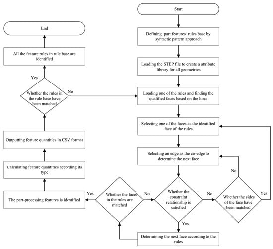
Figure 5. Process of part machining features.

4.3. Feature-Recognition Results

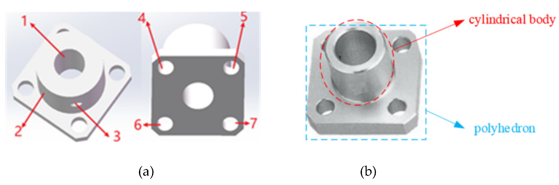
Figure 6 shows a common mechanical part. Its machining features include seven cylindrical faces, one cylindrical body, and one polyhedron. The CSV file results in Table 5 and Table 6, showing the recognition and quantities of features, with machining information extracted from the 2D part drawings. The first and second rows of Table 5 and Table 6 indicate the type of manufacturing feature and its feature quantities, respectively. Additionally, it includes other non-geometric features. The third row indicates the type of geometric features.

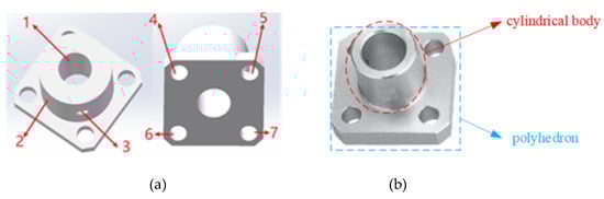
Figure 6. Common mechanical part (a) seven cylindrical faces (b) one cylindrical body and one polyhedron..

Table 5. Shows the results of the first half of the feature recognition and quantities in comma-separated value (CSV) file.

Features Names	Features Number	Two Pins on One Side	Two Sides and One Pin	Hard Facing	Blank Volume	Stiffness Coefficient	Tare Weight	Material Coefficient	Processing Time	Quantity	Ordinary Machine	High Speed Tool	Universal Fixture	Qualification Rate	Total Characteristic	Feature Classes
Characteristic quantity	1000	0	1	2	116,956.5	1.402092	−1	−1	−1	1	1	1	0	1	10	6
Features names	Features number	Is it rotation part	Number of linkage axes	Is it internal or external	Is it concave or convex	Envelope length	Envelope width	Envelope height	Stiffness coefficient	Center of gravity distance	Center of gravity I	Center of gravity J	Center of gravity K	Position coefficient	Characteristic volume	Characteristic Surface Area
BiggestLoop	1	0	2	1	−1	−1	−1	−1	−1	−1	−1	−1	−1	−1	0	0
CylinderHole	7	1	1	−1	0	6.6	6	6.6	1.1	37.21559	−19	32	0	−1	261.36	124.4071
CylinderHole	7	1	1	−1	0	6.6	6	6.6	1.1	37.21559	0	32	19	−1	261.36	124.4071
CylinderHole	7	1	1	−1	0	6.6	6	6.6	1.1	37.21559	19	32	0	−1	261.36	124.4071
CylinderHole	7	1	1	−1	0	6.6	6	6.6	1.1	37.21559	0	32	−19	−1	261.36	124.4071
CylinderHole	7	1	1	−1	0	12.76	35	12.76	2.742947	17.5	0	17.5	0	−1	5698.616	1403.035
GeneralSolid	6	0	3	−1	1	40.07321	6	49.07321	8.178868	32	0	32	0	1	14,449.08	2692.721
Chamfer	34	−1	2	−1	2	−1	−1	−1	−1	−1	−1	−1	−1	−1	0	1026.004
CylinderBoss	22	1	2	−1	1	49.07321	29	49.07321	1.69218	14.5	1.73 × 10−15	14.5	0	1.000001	69,837.23	3220.593

Table 6. Shows the results of the second half of the feature recognition and quantities in comma-separated value (CSV) file.

Hard−to−Process Factor	Volume	Surface Area	Number of Uniaxial Linkage	Uniaxial Momentum	Number of Two−Axis Linkage	Biaxial Momentum	Universal Measuring Tool	2.5 Axis Momentum	Number of 3−Axis Linkage	3-Axis Linkage Momentum	Multiaxial Momentum	Linear Cutting Volume	Electric Spark
1	21,093.36	7632.234	5	6744.056	4	69,837.23	0	0	1	14,449.08	0	0	0
Characteristic of bottom area	Characteristic of depth	Angle of side and bottom face	Angle of side faces	Angle of bottom faces	Characteristic rotation angle	Number of rotations	Curvature	Number	Face Component	Chain Contour Component	Contour length of chain	Processing factor	Precision factor
2,408.18	−1	−1	−1	−1	−1	−1	−1	−1	−1	−1	196.2928	1	1
34.21194	6	−1	−1	−1	3.3	−1	0.3030303	1	1	2	41.46902	1	1
34.21194	6	−1	−1	−1	3.3	−1	0.3030303	1	1	2	41.46902	1	1
34.21194	6	−1	−1	−1	3.3	−1	0.3030303	1	1	2	41.46902	1	1
34.21194	6	−1	−1	−1	3.3	−1	0.3030303	1	1	2	41.46902	1	1
127.8767	35	−1	−1	−1	6.38	−1	0.1567398	1	1	2	80.17345	1	1
669.6201	6	270	−1	−1	−1	0	−1	1	0	2	293.9274	1	1
−1	−1	−1	−1	−1	−1	−1	−1	8	−1	1	48	1	1
2,408.18	29	90	−1	−1	14	−1	0.07142857	1	9	3	315.1703	1	1

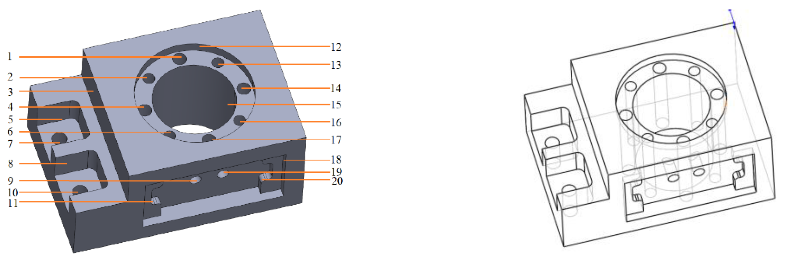
FeatureNet with 3D CNN [30] was used for learning machining features from CAD models of mechanical parts. First, 3D CAD models having machining feature markers were selected, and a large dataset of mechanical parts was composed to train the Fea-tureNet framework of 3D CNN. Subsequently, the 3D CNN could identify manufacturing features from low-level geometric data, as shown in Figure 7. The input CAD component was voxelized using the binvox library. The features subset of features were separated from each other in the voxelized model by using connected component labeling algorithm provided in the scikit-image package for Python. A total of 19 machining features were separated by the watershed segmentation algorithm mentioned in the article. The single segmented features were passed as input into the CNN model for feature recognition. One machining feature was omitted, and 18 machining features were recognized by 3D CNN. Table 7 and Table 8 shows the feature recognition result based on syntactic pattern recognition method. All 20 features of this part are correctly recognized.

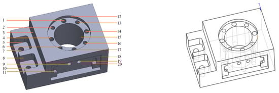
Figure 7. Part features recognized in Zhang’s article (1–20 are features).

Table 7. The first half of the feature recognition results based on syntactic pattern recognition.

Features Names	Features Number	Two Pins on One Side	Two Sides and One Pin	Hard Facing	Blank Volume	Stiffness Coefficient	Tare Weight	Material Coefficient	Processing Time	Quantity	Ordinary Machine	High Speed Tool	Universal Fixture	Qualification Rate	Total Characteristic	Feature Classes
Characteristic quantity	1000	0	1	0	491,220	2.106181	−1	−1	1	1	1	0	0	1	20	7
Features names	Features number	Is it rotation part	Number of linkage axes	Is it internal or external	Is it concave or convex	Envelope length	Envelope width	Envelope height	Stiffness coefficient	Center of gravity distance	Center of gravity I	Center of gravity J	Center of gravity K	Position coefficient	Characteristic volume	Characteristic Surface Area
BiggestLoop	1	0	2	1	−1	−1	−1	−1	−1	−1	−1	−1	−1	−1	0	0
CylinderHole	7	1	1	−1	0	46	6.4	6.4	7.1875	79.4915	28	−36.5151	−64.8194	−1	1884.16	924.8849
CylinderHole	7	1	1	−1	0	46	6.4	6.4	7.1875	51.8543	28	−13.2732	−41.5775	−1	1884.16	924.8849
CylinderHole	7	1	1	−1	0	46	6.4	6.4	7.1875	49.5333	28	−36.5151	−18.3356	−1	1884.16	924.8849
CylinderHole	7	1	1	−1	0	46	6.4	6.4	7.1875	77.9973	28	−59.757	−41.5775	−1	1884.16	924.8849
CylinderHole	7	1	1	−1	0	46	5.6	5.6	8.214286	42.7069	28	−19.7094	−25.5229	−1	1442.56	809.2743
CylinderHole	7	1	1	−1	0	46	5.6	5.6	8.214286	67.4931	28	−20.0806	−59.012	−1	1442.56	809.2743
CylinderHole	7	1	1	−1	0	46	5.6	5.6	8.214286	83.3849	28	−52.9496	−58.012	−1	1442.56	809.2743
CylinderHole	7	1	1	−1	0	46	5.6	5.6	8.214286	64.9602	28	−52.9496	−25.143	−1	1442.56	809.2743
CylinderHole	7	1	1	−1	0	17	7	7	2.428571	119.776	42.5	−52.6911	−98.8116	−1	833	373.8495
CylinderHole	7	1	1	−1	0	17	7	7	2.428571	110.432	42.5	−22.1447	−99.4916	−1	833	373.8495
CylinderHole	7	1	1	−1	0	5.5	11.67673	5.5	2.123042	73.917	26.27772	−59.1918	−35.6305	−1	353.211	180.6205
CylinderHole	7	1	1	−1	0	46	38.24554	38.24554	1.202755	62.0164	28	−36.5151	−41.5775	−1	67,285.17	5476.465
CylinderCavity	27	1	1	−1	0	5	54.72205	54.72205	10.94441	55.3921	2.5	−36.5151	−41.5775	−1	14,972.51	1835.43
CylinderCavity	27	1	1	−1	0	5.5	12.20839	5.5	2.219707	80.7929	26.27772	−58.926	−48.6282	−1	369.3038	187.7931
Notch	27	1	2	−1	1	14	21.89922	18.69065	1.56423	114.288	27	−52.1061	−98.0699	−1	5730.348	1200.753
Notch	46	1	2	−1	1	14	21.89922	18.6516	1.56423	104.4	27	−23.4287	−98.0894	−1	5718.378	1198.805
Notch	46	1	2	−1	1	12.76	5	4	3.1542	45.36	13	−64.32	−64.35	−1	235.65	998.64
Notch	46	1	2	−1	1	12.76	5	4	3.1542	78.36	13	−68.32	−64.35	−1	235.65	954.32

Table 8. The first half of the feature recognition results based on syntactic pattern recognition.

Hard−to−Process Factor	Volume	Surface Area	Number of Uniaxial Linkage	Uniaxial Momentum	Number of Two−Axis Linkage	Biaxial Momentum	Universal Measuring Tool	2.5 Axis Momentum	Number of 3−Axis Linkage	3-Axis Linkage Momentum	Multiaxial Momentum	Linear Cutting Volume	Electric Spark
9	261,298.6	47,074.7	14	97,953.09	5	11,448.73	0	0	1	400,072	0	0	0
Characteristic of bottom area	Characteristic of depth	Angle of side and bottom face	Angle of side faces	Angle of bottom faces	Characteristic rotation angle	Number of rotations	Curvature	Number	Face Component	Chain Contour Component	Contour length of chain	Processing factor	Precision factor
7844.55	−1	90	−1	90	90	1	−1	−1	−1	−1	360.8907	1	1
34.16991	46	90	−1	90	90	1	0.3125	1	1	−1	−1	1	1
34.16991	46	90	−1	90	90	1	0.3125	1	1	−1	−1	1	1
34.16991	46	90	−1	90	90	1	0.3125	1	1	−1	−1	1	1
34.16991	45.99724	90	−1	90	90	1	0.3125	1	1	−1	−1	1	1
24.63009	46	90	−1	90	90	1	0.3571	1	1	−1	−1	1	1
24.63009	46	90	−1	90	90	1	0.3571	1	1	−1	−1	1	1
24.63009	46	90	−1	90	90	1	0.3571	1	1	−1	−1	1	1
24.63009	46	90	−1	90	90	1	0.3571	1	1	−1	−1	1	1
38.48451	17	90	−1	90	90	1	0.2857	1	1	−1	−1	1	1
38.48451	17	90	−1	90	90	1	0.2857	1	1	−1	−1	1	1
23.7583	10.45332	90	−1	90	90	1	0.3637	1	1	−1	−1	1	1
1148.818	45.57951	90	−1	90	90	1	0.0522	1	1	−1	−1	1	1
2351.877	5	90	−1	90	90	1	.0.365	1	9	−1	−1	1	1
23.7583	10.85689	90	−1	90	90	1	0.3636	1	9	−1	−1	1	1
−1	−1	90	180	90	180	2	−1	1	0	−1	−1	1	1
−1	−1	90	180	90	180	2	−1	1	0	−1	−1	1	1
−1	−1	90	180	90	180	2	−1	1	0	−1	−1	1	1
−1	−1	90	180	90	180	2	−1	1	0	−1	−1	1	1

4.4. Data Dimensionality Reduction

The uncertain relationship between feature type and quantities of parts produces two-dimensional data. Principal component analysis method [41] is adopted to compress feature data and reduce data dimension. The principle of this method is to make a linear transformation on the data, and the transformation result is a set of linear independent data representation of each dimension.

For instance, if we assume dataset C consists of s data points with a quantity of features in them, and then denote the vector transpose by T, then we can represent the dataset by normalizing the original matrix C and solving the equation that follows:

$$\mathrm{C}={(C_1,C_2,\dots C_S)}^T,C_i={(C_{\mathrm{i}1},C_{i2},\dots C_{in})}^T,(i=1,2,\dots ,s)$$

(7)

Normalizing the original matrix C:

$$C_m\times \mathrm{n}=\frac{C-mean(C)}{\sqrt{(std(C))}}$$

(8)

Equation solved:

$$(\lambda I-Y)\alpha =0$$

(9)

The above equation yields the eigenvalues ${\lambda }_i$ and eigenvectors ${\alpha }_i(i=1,2,\dots ,n)$ from the covariance matrix $Y_{n\times n}$.

In principal component analysis, determining the principal component requires calculating the contribution rate and cumulative contribution rate, while choosing the appropriate parameter m to obtain the principal component ($P_1,P_2,\dots ,P_m(m\le n)$). Moreover, the principal component can be reduced from N-dimension to m-dimension. In this paper, let m = 1, the contribution rate of the principal component $P_i={\alpha }_i\times C_{s\times n}(i=1,2,\dots ,n)$ be ${\lambda }_i/{\displaystyle \sum _{i=1}^p{\lambda }_i}$, $(i=1,2,\dots ,n)$ and ${\displaystyle \sum _{i=1}^k{\lambda }_i}/{\displaystyle \sum _{i=1}^p{\lambda }_i}$, $(i=1,2,\dots ,n)$ be the cumulative contribution rate.

5. Deep Learning

5.1. CNN Network

CNN is a type of feedforward neural network. Its artificial neurons can respond to the surrounding units within the coverage and have excellent performance in large-scale image processing [42]. With the developments in numerical computing equipment and deep-learning theory, CNNs have been successfully applied in various fields, including image recognition and natural language processing.

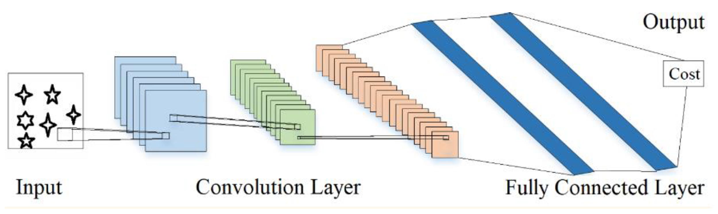
Figure 8 shows a typical convolutional network structure [43]. A convolution layer is used to translate operator to slide the input data up, down, left, and right. In the process of sliding scanning, input data will be aligned by the scanning center of the translation operator, and the scanning results will be weighted.

Figure 8. Structure of the CNN.

In the convolution layer, each layer extracts features of the input data, high-level convolution layer extracts more abstract and complex features, which include the local and overall features of the data. The convolution unit weights the parameters and continuously optimizes the weight through the back-propagation algorithm, to adjust the output and continuously reduce the difference between input and output.

$${\mathrm{P}}^{l+1}(i,j)=[P^l\otimes w^l](i,j)+b={\displaystyle \sum _{m=1}^{M_l}{\displaystyle \sum _{x=1}^f{\displaystyle \sum _{y=1}^f[P_m^l(s_{0}i+x,s_{0}j+y)w_m^{l+1}(x,y)]+b}}}$$

(10)

$$(i+j)\in \{0,1,\dots L_{l+1}\}$$

(11)

$$L_{l+1}=\frac{L_l+2n-f}{s_0}+1$$

(12)

In the above equation, P (i, j) and M are the pixel value and number of channels of the graph, respectively; P^l is the convolution input of the next layer, and P^l+1 is the output of P^l; L_l+1 is the size of the output of layer l + 1; b is the bias term; s₀, n, and f are the number of convolution layers respectively.

The function of full connection layer is to connect each node with all nodes of the previous layer, which is used to synthesize the features extracted by convolution layer.

$${\mathrm{P}}^{l+1}={\displaystyle \sum _{m=1}^{M_l}{\displaystyle \sum _{x=1}^f{\displaystyle \sum _{y=1}^f(Z_{i,j,m}^l{w}_m^{l+1})+b=w_{l+1}^T{P}_{l+1}+b}}}$$

(13)

$$L_l=L_{l+1}$$

(14)

Pooling layer is used to compress features and reduce the memory consumption by down sampling to reduce the dimension and remove the redundant information.

$$A_k^l(i,j)={[{\displaystyle \sum _{x=1}^f{\displaystyle \sum _{y=1}^f{A}_k^l{(s_{0}i+x,s_{0}j+y)}^n}}]}^{\frac{1}{n}}$$

(15)

Here, s₀ is step size, and n represents the pre-specified parameters.

In this study, the quotation problem was a regression problem, the inputs of the network were the feature-quantity data and real cost, and the output was the predicted cost. The activation function used in this network was the rectified linear unit (ReLU). The ReLU sparse model can mine relevant features and fit the training data.

5.2. Training Data

Ubuntu18.04 operating system is conducted in this experiment, and the GPU is GeForce 1080 Ti memory with 11 GB. The input data for the CNN was built from TensorFlow and written in Python, with the convolution kernel initialized by a random fractional number. The configuration information is listed in Table 9, which includes the network structure. The experimental data included 47,861 STEP files.

Table 9. Configuration information and training hyperparameters.

Convolutional Neural Network (CNN)				Back Propagation (BP) Network
Structure	Layer (Type)	Output Shape	Param	Output Shape	Param
Convolution	Con2d_1	30, 30, 64	37,568	\	\
	Con2d_2	15, 15, 128	221,440	\	\
	Con2d_3	8, 8, 256	885,248	\	\
	Con2d_4	4, 4, 512	3,539,968	\	\
	Con2d_5	2, 2, 512	4,719,616	\	\
Fully connected	dense_1	4096	2,101,248	4096	217,088
	dense_2	4096	16,781,312	4096	16,781,312
	dense_3	1	4097	4096	4,097,000
	dense_4	\	\	1	1001

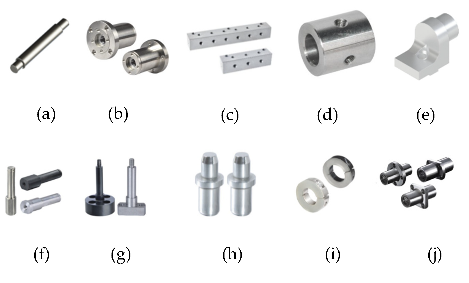
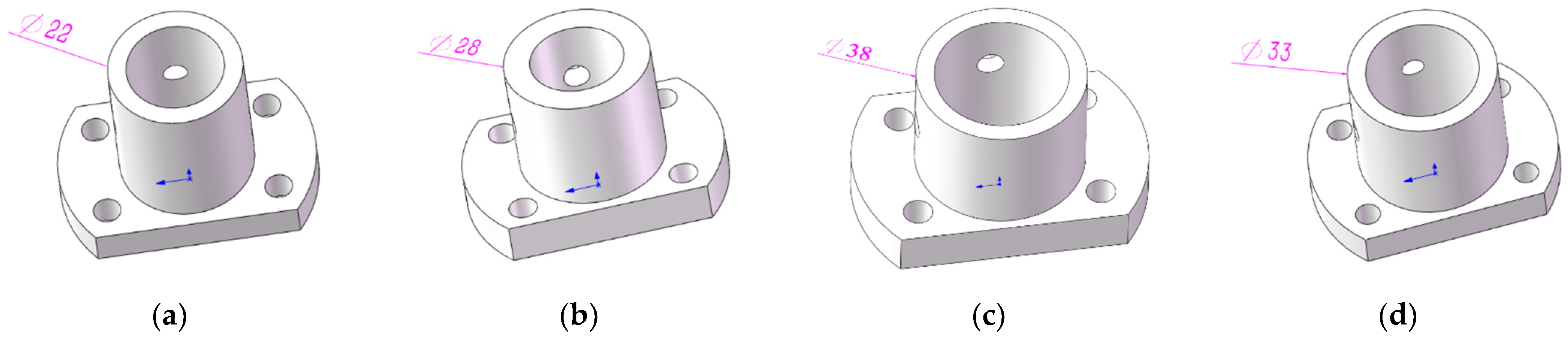
Some actual parts are shown in Figure 9. To improve the accuracy of the quotation, it was necessary to expand the data. In the STEP file, the size of the part was changed according to the feature quantity; thus, different cost and feature quantities were obtained to make the loss converge more easily during the training phase. For example, as shown in Figure 10, the diameter length of the guide shaft bearing was extended to 22 mm, 28 mm, 33 mm, and 38 mm, respectively. The costs of these four sizes of guide shaft bearing are $10.61, $10.77, $10.89, and $11.04, respectively.

Figure 9. Some actual 3D parts(a–j represent different parts).

Figure 10. Variation of axis diameter and length of bearings with different guiding shafts.

Through recognition of the syntactic pattern features and extraction of the processing information of the corresponding 2D processing drawings, a dataset of 117,708 CSV files with feature quantities was obtained, along with the corresponding part costs. The part costs were the average costs given by quoters. As the input data size of the CNN was fixed, the features and feature quantities of the parts were changed. There were generally less than thirty part features and feature quantities for the research object. Therefore, the size of the CNN was set to 30 × 30. Insufficient to fill in −1.

The data set is divided into training dataset (60%), test dataset (20%), and validation dataset (20%) respectively. This CNN was trained on a training dataset, validated on a validation dataset, and tested on a test dataset.

5.3. Analysis of Results

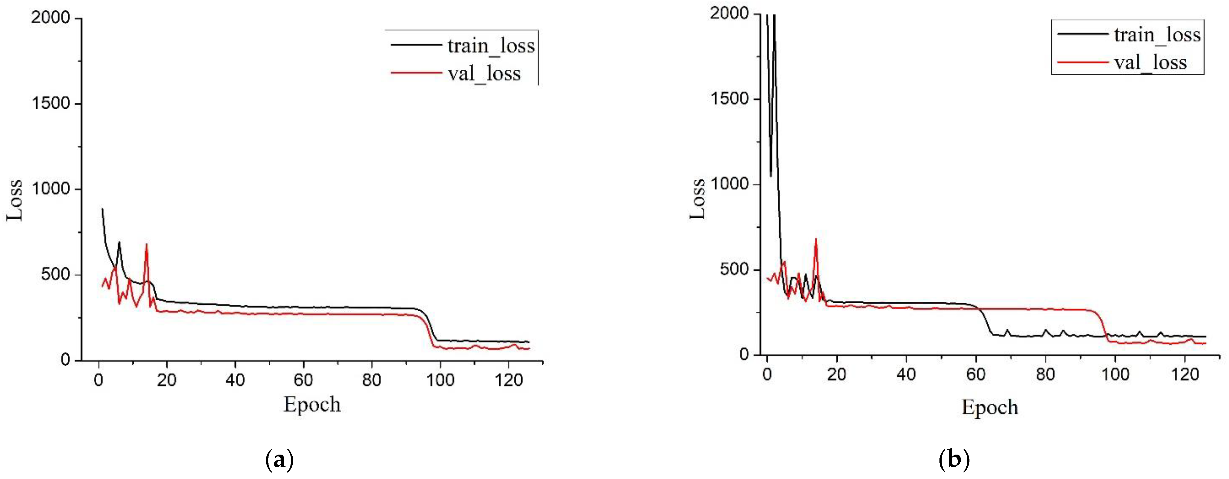
Figure 11 shows a comparison of two optimizers—stochastic gradient descent (SGD) and RMSProp—with regard to the training and validation losses by the CNN network. The SGD optimizer only calculated the gradient for one random sample at each iteration until convergence. The RMSProp algorithm takes an exponentially weighted moving average of the gradients by the square of the elements. This approach is advantageous for eliminating directions with large oscillations and for correcting the oscillations so that they become smaller in each dimension. Additionally, the network function converged faster. The initial learning rates of the SGD and RMSProp optimizers were set to 0.00001 and 0.001, respectively. The results for SGD and RMSProp are presented in Figure 11a,b, respectively, with regard to the validation loss and validation accuracy. For the RMSProp optimizer, after 127 epochs, the loss function tended to be stable, and the train-loss was 106.91. However, for the SGD optimizer, after 127 epochs, the train-loss was 130.76, and there was no longer convergence. In the training process, the learning rate of the model was adjusted to 0.1 times the previous one if the model did not converge in five consecutive attempts.

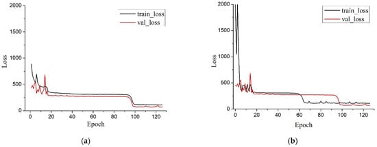
Figure 11. CNN network convergence of the loss functions. (a) RMSProp optimizer; (b) SGD optimizer.

Figure 12 shows that the BP network convergence of the RMSProp optimizer’s loss functions was observed. After 35 epochs, the loss function tended to be stable, and the train-loss was 112.85. By comparing the BP network and CNN network, it can be concluded that CNN network converges better, although it takes a little longer to train.

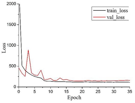
Figure 12. BP network convergence of the loss functions of RMSProp optimizer.

To measure accuracy, the “man absolute percentage error” was adopted. It is an optimization of the mean absolute error into a percentage value, with a more accurate and understandable prediction accuracy.

$$MAPE=\frac{100\%}{n}{\displaystyle \sum _{i=1}^n\left|\frac{{\widehat{y}}_i-y_i}{y_i}\right|}$$

(16)

In the above, $y_i$ represents the real cost of the parts, and ${\widehat{y}}_i$ represents the predicted cost from the trained model.

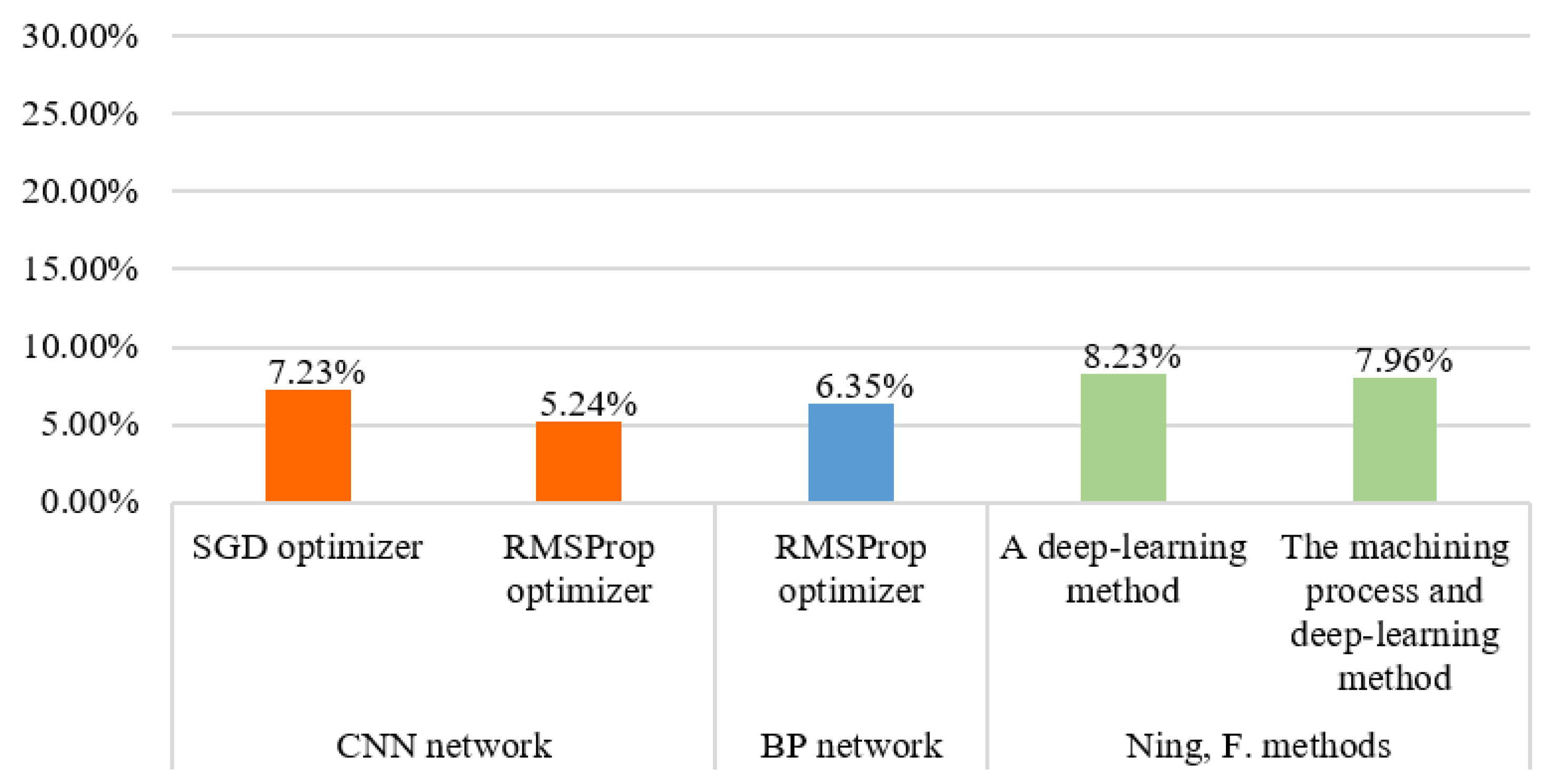
From the value of the mean absolute percentage error (MAPE) shown in Figure 13, one can conclude that the model trained by than RMSProp optimizer is better than the model trained by the SGD optimizer for the CNN network. RMSProp exhibited a better convergence process than SGD. Thus, the RMSProp optimizer was more suitable for obtaining an applicable training model. By comparing the CNN and BP networks, it can be concluded that the respective estimation effects of the two networks are good; however, the CNN network has a more accurate estimation effect.

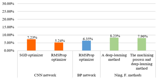
Figure 13. MAPEs for different methods.

The cost estimation methods in article [44,45] are compared with the method proposed in this paper. Using the same dataset, the MAPEs results are shown in Figure 13. In article [44], a regression analysis of cost and part voxel data was performed using a 3D CNN. In article [45], a regression analysis of cost and feature quantities were performed using a feature recognition method combining graph theory and deep learning. Both methods studied the correlation between cost and geometric features but did not fully consider the characteristic quantity of the machining process. Therefore, the research method in this paper has better accuracy.

6. Conclusions

A cost estimation method using feature-based and process-based budgeting has high estimation accuracy but requires accurate identification of the machining features and establishes a correlation between the cost and features quantities. This paper proposes a feature recognition method based on syntactic pattern recognition in view of the problem of inaccurate recognition of existing feature recognition methods for part processing. The proposed method made the feature definition more precise and easily described complex features by using feature constraints of parts. With particular regard to recognition efficiency, this study provided clue hints and direction search methods, making the feature matching more efficient and flexible.

In addition, to establish the relationships between the geometric features, processing modes, and the costs of parts, this study proposed a method of describing the features and the processing mode using feature quantities. Using the method of identifying machining features to calculate the quantity and save it as CSV data, the formalization of features is completed to assign a value to the part machining features, resulting in an overall description of the part machining features.

Finally, deep learning technology was adopted to establish the relationships between feature quantities and cost. By comparing two different networks, i.e., BP and CNN networks, it was concluded that they both had improved training effects, but the CNN network had the best performance. The RMSProp optimizer exhibited a high accuracy and was more suitable than the SGD optimizer for obtaining an applicable training model.

The recognition of intersecting features is a constant problem that cannot always be solved by all types of feature recognition methods. The method proposed herein has great potential for solving the problem of intersecting features, as it can perfectly describe the features using a syntactic pattern. There are many factors that affect the costs of parts in the overall design and manufacturing process. This study does not examine all influencing factors of each process, rather provides a method to estimate the cost of parts. Future research will focus on all the factors in a manufacturing process.

References

- Hsieh, I.-Y.L.; Pan, M.S.; Chiang, Y.-M.; Green, W.H. Learning only buys you so much: Practical limits on battery price reduction. Appl. Energy 2019, 239, 218–224. [Google Scholar] [CrossRef]
- Hanchate, D.B.; Hassankashi, M. ANN with Fuzzification in Software Cost Estimation. Emerg. Issues Sci. Technol. 2020, 3, 139–150. [Google Scholar]
- Hashemi, S.T.; Ebadati E., O.M.; Kaur, H. A hybrid conceptual cost estimating model using ANN and GA for power plant projects. Neural Comput. Appl. 2019, 31, 2143–2154. [Google Scholar] [CrossRef]
- Wouters, M.; Stecher, J. Development of real-time product cost measurement: A case study in a medium-sized manufacturing company. Int. J. Prod. Econ. 2017, 183, 235–244. [Google Scholar] [CrossRef]
- Jin, X.; Ji, Y.; Qu, S. Minimum cost strategic weight assignment for multiple attribute decision-making problem using robust optimization approach. Comput. Appl. Math. 2021, 40, 193. [Google Scholar] [CrossRef]
- Liu, Y.; Dong, Y.; Liang, H.; Chiclana, F.; Herrera-Viedma, E. Multiple attribute strategic weight manipulation with minimum cost in a group decision making context with interval attribute weights information. IEEE Trans. Syst. Man Cybern. Syst. 2018, 49, 1981–1992. [Google Scholar] [CrossRef]
- Ganorkar, A.B.; Lakhe, R.R.; Agrawal, K.N. Cost estimation techniques in manufacturing industry: Concept, evolution and prospects. Int. J. Econ. Account. 2018, 8, 303–336. [Google Scholar] [CrossRef]
- Relich, M.; Pawlewski, P. A case-based reasoning approach to cost estimation of new product development. Neurocomputing 2018, 272, 40–45. [Google Scholar] [CrossRef]
- Campi, F.; Favi, C.; Mandolini, M.; Germani, M. Using design geometrical features to develop an analytical cost estimation method for axisymmetric components in open-die forging. Procedia CIRP 2019, 84, 656–661. [Google Scholar] [CrossRef]
- Schmidt, T. Potentialbewertung Generativer Fertigungsverfahren für Leichtbauteile; Springer Science and Business Media: Berlin/Heidelberg, Germany, 2016. [Google Scholar]
- Lin, C.-K.; Shaw, H.-J. Feature-based estimation of preliminary costs in shipbuilding. Ocean Eng. 2017, 144, 305–319. [Google Scholar] [CrossRef]
- Henderson, M.R.; Anderson, D.C. Computer Recognition and Extraction of Form Features. Comput. Ind. 1984, 5, 329–339. [Google Scholar] [CrossRef]
- Grabowik, C. Metodyka Integracji Funkcji Technicznego Przygotowania Produkcji; Wydawnictwo Politechniki Śląskiej: Gliwice, Poland, 2013. [Google Scholar]
- Joshi, S.; Chang, T. Graph-based heuristics for recognition of machined features from a 3D solid model. Comput. Des. 1988, 20, 58–66. [Google Scholar] [CrossRef]
- Weise, J.; Benkhardt, S.; Mostaghim, S. A Survey on Graph-based Systems in Manufacturing Processes. In Proceedings of the 2018 IEEE Symposium Series on Computational Intelligence (SSCI), Bangalore, India, 8–21 November 2018; pp. 112–119. [Google Scholar] [CrossRef]
- Malyshev, A.; Slyadnev, S.; Turlapov, V. Graph-based feature recognition and suppression on the solid models. GraphiCon 2017, 17, 319–322. [Google Scholar]
- Venuvinod, P.; Wong, S. A graph-based expert system approach to geometric feature recognition. J. Intell. Manuf. 1995, 6, 401–413. [Google Scholar] [CrossRef]
- Yuen, C.F.; Venuvinod, P. Geometric feature recognition: Coping with the complexity and infinite variety of features. Int. J. Comput. Integr. Manuf. 2010, 12, 439–452. [Google Scholar] [CrossRef]
- Dong, X.; Wozny, M.J. A method for generating volumetric features from surface features. Int. J. Comput. Geom. Appl. 1991, 1, 281–297. [Google Scholar] [CrossRef]
- Wang, E.; Kim, Y.S. Form feature recognition using convex decomposition: Results presented at the 1997 asme cie feature panel session. Comput. Des. 1998, 30, 983–989. [Google Scholar] [CrossRef]
- Gupta, M.K.; Swain, A.K.; Jain, P.K. A novel approach to recognize interacting features for manufacturability evaluation of prismatic parts with orthogonal features. Int. J. Adv. Manuf. Technol. 2019, 105, 343–373. [Google Scholar] [CrossRef]
- Deng, B.; Genova, K.; Yazdani, S.; Bouaziz, S.; Hinton, G.; Tagliasacchi, A. Cvxnet: Learnable convex decomposition. In Proceedings of the 2020 IEEE/CVF Conference on Computer Vision and Pattern Recognition (CVPR), Salt Lake City, Utah, 18–22 June 2020; pp. 31–41. [Google Scholar]
- Vandenbrande, J.; Requicha, A.A. Spatial reasoning for the automatic recognition of machinable features in solid models. IEEE Trans. Pattern Anal. Mach. Intell. 1993, 15, 1269–1285. [Google Scholar] [CrossRef]
- Li, Z.; Lin, J.; Zhou, D.; Zhang, B.; Li, H. Local Symmetry Based Hint Extraction of B-Rep Model for Machining Feature Recognition. In Proceedings of the ASME 2018 International Design Engineering Technical Conferences and Computers and Information in Engineering Conference, Quebec City, QC, Canada, 26–29 August 2018; p. V004T05A009. [Google Scholar]
- Li, Z.; Lin, Z.; He, D.; Tian, F.; Qin, T.; Wang, L.; Liu, T.-Y. Hint-based Training for Non-Autoregressive Machine Translation; Association for Computational Linguistics: Hong Kong, China, 2019; pp. 5712–5717. [Google Scholar]
- Ghadai, S.; Balu, A.; Sarkar, S.; Krishnamurthy, A. Learning localized features in 3D CAD models for manufacturability analysis of drilled holes. Comput. Aided Geom. Des. 2018, 62, 263–275. [Google Scholar] [CrossRef]
- Su, H.; Maji, S.; Kalogerakis, E.; Learned-Miller, E. Multi-view convolutional neural networks for 3d shape recognition. In Proceedings of the IEEE International Conference on Computer Vision, Santiago, Chile, 7–13 December 2015; pp. 945–953. [Google Scholar]
- Ghadai, S.; Lee, X.; Balu, A.; Sarkar, S.; Krishnamurthy, A. Multi-Resolution 3D Convolutional Neural Networks for Object Recognition. Comput. Vis. Pattern Recognit. 2018, arXiv:1805.122544. [Google Scholar]
- Maturana, D.; Scherer, S. Voxnet: A 3d convolutional neural network for real-time object recognition. In Proceedings of the 2015 IEEE/RSJ International Conference on Intelligent Robots and Systems (IROS), Hamburg, Germany, 28 September–2 October 2015; pp. 922–928. [Google Scholar]
- Zhang, Z.; Jaiswal, P.; Rai, R. Featurenet: Machining feature recognition based on 3d convolution neural network. Comput.-Aided Des. 2018, 101, 12–22. [Google Scholar] [CrossRef]
- Shi, Y. Manufacturing Feature Recognition With 2D Convolutional Neural Networks. Master’s Thesis, University of South Carolina, Columbia, SC, USA, 2018. Available online: https://scholarcommons.sc.edu/etd/5100/ (accessed on 5 March 2019).
- Shi, Y.; Zhang, Y.; Baek, S.; De Backer, W.; Harik, R. Manufacturability analysis for additive manufacturing using a novel feature recognition technique. Comput. Des. Appl. 2018, 15, 941–952. [Google Scholar] [CrossRef]
- Ranjan, R.; Kumar, N.; Pandey, R.K.; Tiwari, M. Automatic recognition of machining features from a solid model using the 2d feature pattern. Int. J. Adv. Manuf. Technol. 2005, 26, 861–869. [Google Scholar] [CrossRef]
- Subrahmanyam, S.; Wozny, M. An overview of automatic feature recognition techniques for computer-aided process planning. Comput. Ind. 1995, 26, 1–21. [Google Scholar] [CrossRef]
- Malhan, R.K.; Kabir, A.M.; Shah, B.; Gupta, S.K. Identifying feasible workpiece placement with respect to redundant manipulator for complex manufacturing tasks. In Proceedings of the 2019 International Conference on Robotics and Automation (ICRA), Montreal, Canada, 20–24 May 2019; pp. 5585–5591. [Google Scholar]
- Chen, C.H. Handbook of Pattern Recognition and Computer Vision; World Scientific: Singapore, 2015. [Google Scholar]
- Flasiński, M. Syntactic pattern recognition: Paradigm issues and open problems. In Handbook of Pattern Recognition and Computer Vision; World Scientific Pub Co Pte Ltd.: Singapore, 2016; pp. 3–25. [Google Scholar]
- Flasiński, M.; Jurek, J. Fundamental methodological issues of syntactic pattern recognition. Pattern Anal. Appl. 2013, 17, 465–480. [Google Scholar] [CrossRef] [Green Version]
- Capoyleas, V.; Chen, X.; Hoffmann, C.M. Generic naming in generative constraint-based design. Comput. Des. 1996, 28, 17–26. [Google Scholar] [CrossRef] [Green Version]
- Feng, C.X.; Kusiak, A. Constraint-based design of parts. Comput. Des. 1995, 27, 343–352. [Google Scholar] [CrossRef]
- Aït-Sahalia, Y.; Xiu, D. Principal component analysis of high-frequency data. J. Am. Stat. Assoc. 2019, 114, 287–303. [Google Scholar] [CrossRef] [Green Version]
- Goodfellow, I.; Bengio, Y.; Courville, A. Deep Learning Cambridge; MIT Press: Cambridge, MA, USA, 2016; pp. 326–366. [Google Scholar]
- Gu, J.; Wang, Z.; Kuen, J.; Ma, L.; Shahroudy, A.; Shuai, B.; Liu, T.; Wang, X.; Wang, G.; Cai, J.; et al. Recent advances in convolutional neural networks. Pattern Recognit. 2018, 77, 354–377. [Google Scholar] [CrossRef] [Green Version]
- Ning, F.; Shi, Y.; Cai, M.; Xu, W.; Zhang, X. Manufacturing cost estimation based on a deep-learning method. J. Manuf. Syst. 2020, 54, 186–195. [Google Scholar] [CrossRef]
- Ning, F.; Shi, Y.; Cai, M.; Xu, W.; Zhang, X. Manufacturing cost estimation based on the machining process and deep-learning method. J. Manuf. Syst. 2020, 56, 11–22. [Google Scholar] [CrossRef]
Publisher’s Note: MDPI stays neutral with regard to jurisdictional claims in published maps and institutional affiliations. |
© 2022 by the authors. Licensee MDPI, Basel, Switzerland. This article is an open access article distributed under the terms and conditions of the Creative Commons Attribution (CC BY) license (https://creativecommons.org/licenses/by/4.0/).