Orientation Asymmetric Surface Model for Membranes: Finsler Geometry Modeling

Abstract

We study triangulated surface models with nontrivial surface metrices for membranes. The surface model is defined by a mapping $\mathbf{r}$ from a two-dimensional parameter space M to the three-dimensional Euclidean space ${\mathbf{R}}^3$. The metric variable $g_{ab}$, which is always fixed to the Euclidean metric ${\delta }_{ab}$, can be extended to a more general non-Euclidean metric on M in the continuous model. The problem we focus on in this paper is whether such an extension is well defined or not in the discrete model. We find that a discrete surface model with a nontrivial metric becomes well defined if it is treated in the context of Finsler geometry (FG) modeling, where triangle edge length in M depends on the direction. It is also shown that the discrete FG model is orientation asymmetric on invertible surfaces in general, and for this reason, the FG model has a potential advantage for describing real physical membranes, which are expected to have some asymmetries for orientation-changing transformations.

1. Introduction

Biological membranes including artificial ones, such as giant vesicles, are simply understood as two-dimensional surfaces [1]. The well-known surface model for membranes is statistical mechanically defined by using a mapping $\mathbf{r}$ from a two-dimensional parameter space M to ${\mathbf{R}}^3$ [2]. This mapping $\mathbf{r}$ and the metric $g_{ab}(a,b=1,2)$, a set of functions on M, are the dynamical variables of the model. To discretize these dynamical variables, we use triangulated surfaces in both M and ${\mathbf{R}}^3$. On the discrete surfaces, the metric $g_{ab}$ is always fixed to the Euclidean metric ${\delta }_{ab}$ [3,4,5], while the induced metric ${\partial }_a\mathbf{r}·{\partial }_b\mathbf{r}$ is also used in theoretical studies on continuous surfaces [2]. These two-dimensional surface models are considered as a natural extension of the one-dimensional polymer model [6], and many studies for membranes have been conducted [7,8,9,10,11]. Landau–Ginzburg theory for membranes has also been developed [12]. In [13], the anisotropic morphologies of membranes are studied, and the notion of the multi-component is essential also for scalar functions, which are used to define the metric function on the triangles [14].

However, it is still unclear whether the non-Euclidean metric can be assumed or not for discrete models. In this paper, we study the metric $g_{ab}$ in [13] in more detail. We will show that models with the metric in [13] and their extension to a more general one are ill-defined in the ordinary surface modeling prescription; however, these ill-defined models turn out to be well-defined in the context of Finsler geometry (FG) modeling [15,16,17,18,19,20]. Moreover, it is also shown that the FG model becomes orientation asymmetric, where “orientation asymmetric” means that the Hamiltonian is not invariant under the surface inversion [13]. In real physical membranes, the orientation asymmetry is observed because of their bilayer structure [21]. Indeed, asymmetry such as area difference between the outer and inner layers is expected to play an important role for the anisotropic shape of membranes. Therefore, it is worthwhile to study the discrete surface model with non-trivial metric $g_{ab}$ more extensively.

We should note that there are two types of discrete surface models; the first is the fixed connectivity (FC), model and the second is the dynamically triangulated (DT) surface model. The FC surface model corresponds to polymerized membranes, while the DT surface model corresponds to fluid membranes, such as bilayer vesicles. The polymerized and fluid membranes are characterized by nonzero and zero shear moduli, respectively. Numerically, the dynamical triangulation for the DT models is simulated by the bond-flip technique as one of the Monte Carlo processes on triangulated lattices [22,23,24], while the FC surface models are defined on triangulated lattices without the bond flips. According to this classification, the discrete models in this paper belong to the DT surface models and correspond to fluid membranes, because the dynamical triangulation is assumed in the partition function, which will be defined in Section 3, just like in the model of [13].

In Section 2, a continuous surface model and its basic properties are reviewed, and a non-Euclidean metric, which we study in this paper, is introduced. In Section 3, we discuss why orientation asymmetry needs to be studied, and then, we introduce a discrete model on a triangulated spherical lattice and show that this discrete model is ill-defined in the ordinary context of surface modeling. In Section 4, we show that this ill-defined model can be understood as a well-defined FG model in a modeling that is slightly extended from the one in [15]. In Section 5, we summarize the results.

2. Continuous Surface Model

In this paper, we study a surface model that is an extension of the Helfrich and Polyakov (HP) model [25,26]. The HP model is physically defined by Hamiltonian S, which is a linear combination of the Gaussian bond potential $S_1$ and the bending energy $S_2$ such that:

$$\begin{array}{c}\hfill \begin{array}{c}S=S_1+\kappa S_2,\hfill \\ S_1=\int \sqrt{g}{d}^{2}x{g}^{ab}\frac{\partial \mathbf{r}}{\partial x_a}·\frac{\partial \mathbf{r}}{\partial x_b},\hfill \\ S_2=\frac{1}{2}\int \sqrt{g}{d}^{2}x{g}^{ab}\frac{\partial \mathbf{n}}{\partial x_a}·\frac{\partial \mathbf{n}}{\partial x_b},\hfill \end{array}\end{array}$$

(1)

where $\kappa \left[k_{B}T\right]$ is the bending rigidity ($k_B$ and T are the Boltzmann constant and the temperature, respectively). The surface position is described by $\mathbf{r}(\in {\mathbf{R}}^3)$, and $g_{ab}$ is a Riemannian metric on the two-dimensional surface M; $g^{ab}\left(={\left(g_{ab}\right)}^{-1}\right)$ is its inverse; and $g=det{g}_{ab}$. Note that the surface position $\mathbf{r}$ is understood as a mapping $\mathbf{r}:M\ni x=(x_1,x_2)\mapsto \left(X\left(x\right),Y\left(x\right),Z\left(x\right)\right)\in {\mathbf{R}}^3$, where the surface orientation is assumed to be preserved. The symbol $\mathbf{n}$ in $S_2$ denotes a unit normal vector of the image surface, where one of two orientations is used to define $\mathbf{n}$.

It is well known that the Hamiltonian is invariant under (i) general coordinate transformation $x\to x^{\prime }$ in M and (ii) conformal transformation for $g_{ab}$ such that $g_{ab}\to g_{ab}^{\prime }=f\left(x\right)g_{ab}$ with a positive function f on M [2]. The first property under the transformation (i), called re-parametrization invariance, is expressed by $S(\mathbf{r}\left(x\right),g_{ab}\left(x\right))=S(\mathbf{r}\left(x^{\prime }\right),g_{ab}\left(x^{\prime }\right))$, where $\mathbf{r}\left(x^{\prime }\right)$ and $g_{ab}\left(x^{\prime }\right)$ are composite functions. The second property under (ii) is expressed by $S(\mathbf{r}\left(x\right),g_{ab}\left(x\right))=S(\mathbf{r}\left(x\right),g_{ab}^{\prime }\left(x\right))$. The metrices $g_{ab}$ and $g_{ab}^{\prime }$ are called conformally equivalent, which is written as $g_{ab}\simeq g_{ab}^{\prime }$, if there exists a positive function f such that $g_{ab}^{\prime }=f{g}_{ab}$. Therefore, the second property with respect to the transformation (ii) implies that S depends only on conformally non-equivalent metrices.

The metric $g_{ab}$ of the surface M is generally given by $g_{ab}=\left(\begin{array}{cc}\hfill E& \hfill F\\ \hfill F& \hfill G\end{array}\right)$ with the functions of $E>0,G>0,EG-F^2>0$. By letting $F=0$, we have $g_{ab}=\left(\begin{array}{cc}\hfill E& \hfill 0\\ \hfill 0& \hfill G\end{array}\right)=E\left(\begin{array}{cc}\hfill 1& \hfill 0\\ \hfill 0& \hfill G/E\end{array}\right)\simeq \left(\begin{array}{cc}\hfill 1& \hfill 0\\ \hfill 0& \hfill {\rho }^2\end{array}\right)\simeq \left(\begin{array}{cc}\hfill 1/\rho & \hfill 0\\ \hfill 0& \hfill \rho \end{array}\right)$, where ${\rho }^2=G/E$ [13]. This metric is in general not conformally equivalent to the Euclidean metric ${\delta }_{ab}$. We call a metric $g_{ab}$ trivial (non-trivial) if $g_{ab}$ is conformally equivalent (inequivalent) to ${\delta }_{ab}$, although surface models with $g_{ab}={\delta }_{ab}$ and $g_{ab}={\partial }_a\mathbf{r}·{\partial }_b\mathbf{r}$ are physically non-trivial [22,23,24,27,28,29,30,31,32].

3. Discrete Surface Model

3.1. Membrane Orientation

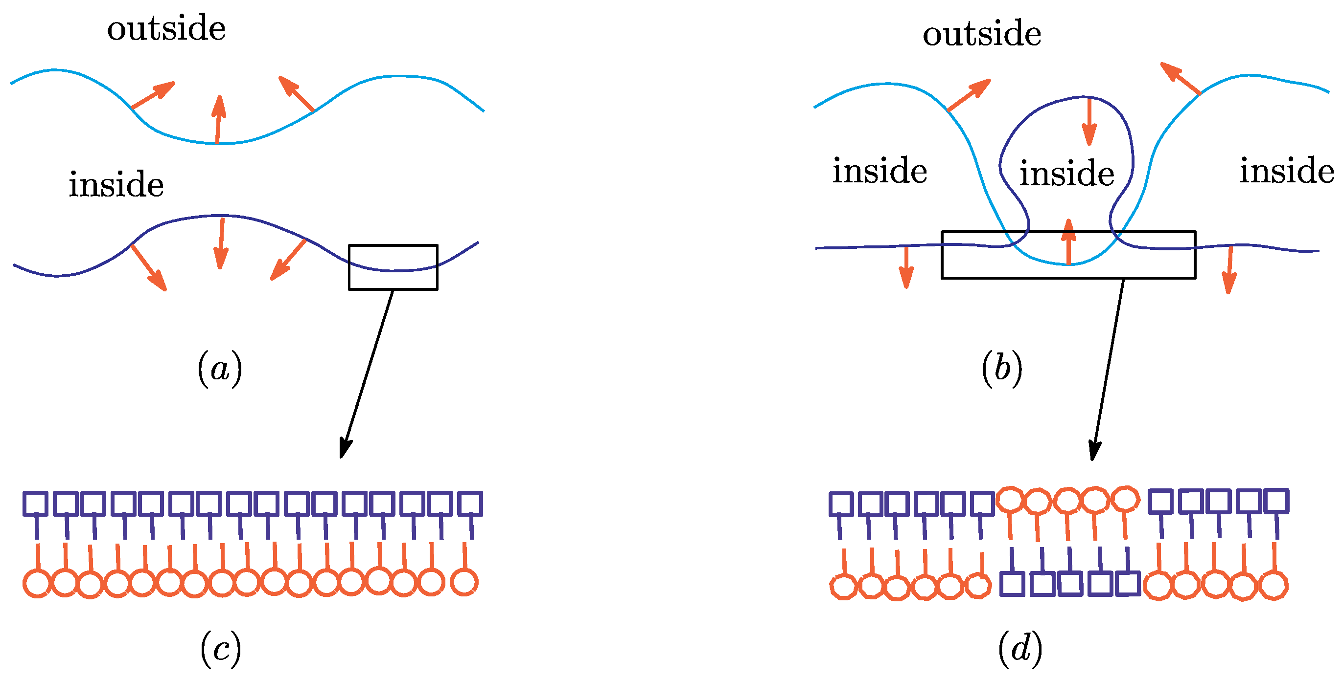
First, we should comment on the surface orientation. The unit normal vector $\mathbf{n}$ is directed from inside to outside of the material separated from bulk material by the membrane (see Figure 1a). However, if the membrane self-intersects, then the direction of $\mathbf{n}$ changes from outside to inside (Figure 1b). Otherwise (⇔$\mathbf{n}$ is directed from inside to outside), $\mathbf{n}$ discontinuously changes at the intersection point. For this reason, we change the surface orientation by changing the local coordinate system from left-handed to right-handed while $\mathbf{n}$ remains unchanged (Figure 1b). We should emphasize that our basic assumption is that the surface orientation is locally changeable. This means that the surface in ${\mathbf{R}}^3$ is self-intersecting, or in other words, the surface is not self-avoiding.

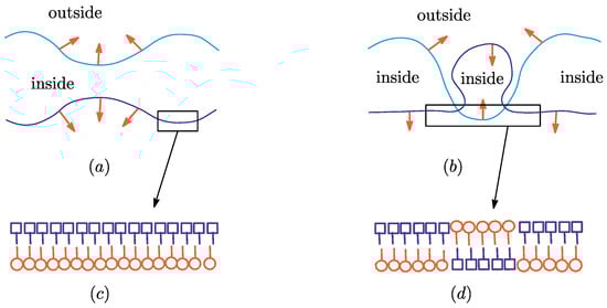
Figure 1. A membrane in aqueous solution separates the solution into two regions; inside and outside. (a) Self-avoiding surface with unit normal vectors $\mathbf{n}$; (b) self-intersecting surface with $\mathbf{n}$; (c) lipid bilayer structure of membranes, where the symbols of lipids for inner and outer layers are drawn differently; and (d) a partly inverted bilayer.

However, such an intersection process is not so easy to implement in the numerical simulations (no numerical simulation is performed in this paper). Apart from this, it is unclear whether or not the implementation of such an intersection process is effective for simulating the membrane inversion. Therefore, we assume that the surface is locally invertible without intersections; an inversion is expected to occur independent of whether the surface is self-intersecting or not. Indeed, real physical membranes are composed of lipid molecules, which have hydrophobic and hydrophilic parts. These lipids form a bilayer structure (Figure 1c). In those real membranes, the bilayer structure is partly inverted just as in Figure 1d via the so-called flip-flop process. Such an inversion process without intersection is not always unphysical because it can be seen in the process of pore formation. The pore formation process is reversible and forms cup-like membranes, where the membranes are not always self-intersecting [33]. The cup-like membranes are stable [34] and expected to play an important role as an intermediate configuration for cell inversion. It should be remarked that the surface orientation is also changeable in the process of cell fission and fusion, where the surface self-intersects, in real physical membranes.

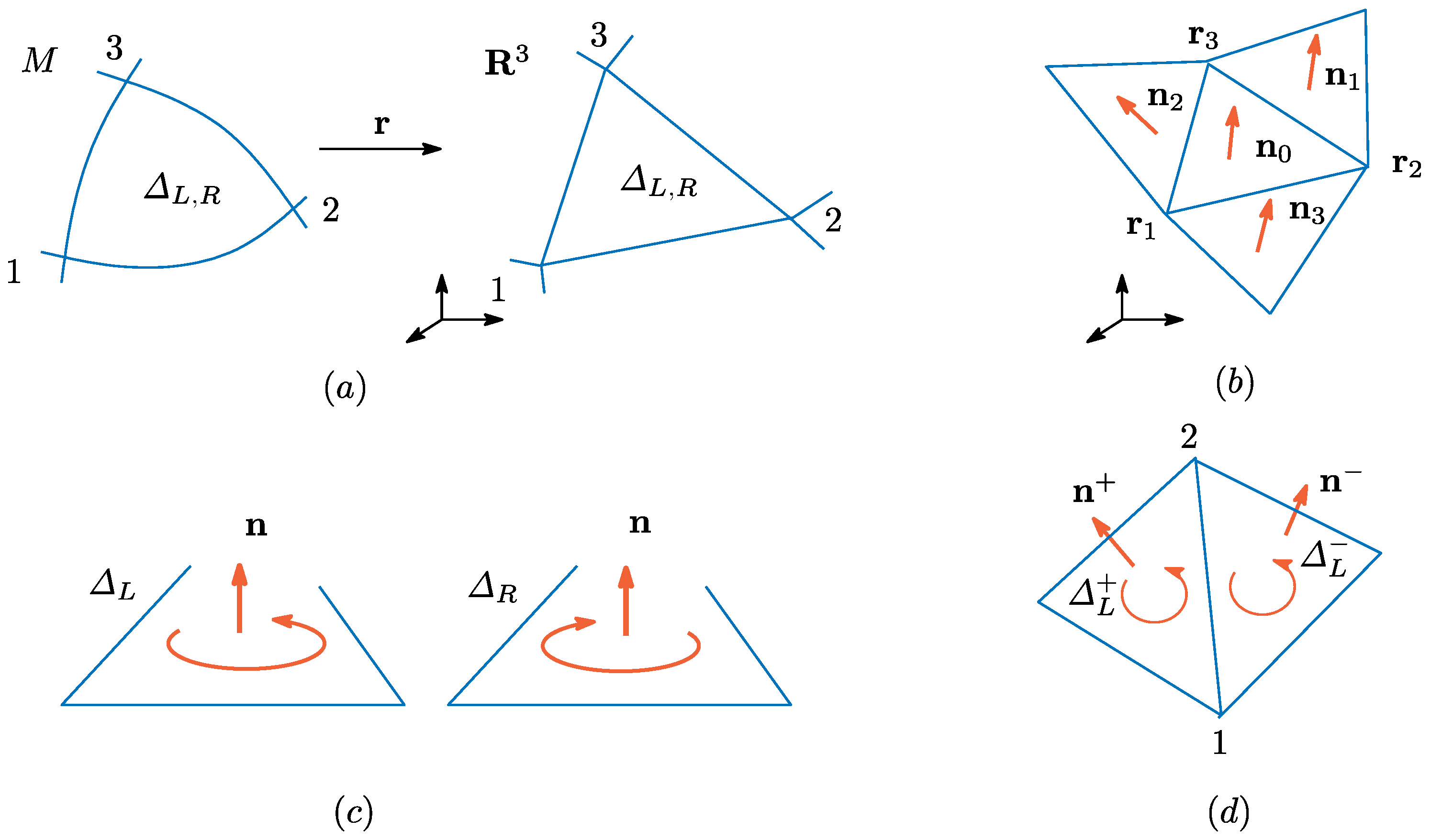
To define a discrete model, we use a piecewise-linearly triangulated surface in ${\mathbf{R}}^3$ [3,4,5]. In this paper, a spherical surface is assumed. Therefore, it is natural to assume that M is also triangulated and of sphere topology. Triangles in M can be smooth in general, and these smooth triangles are mapped to piecewise-linear triangles in ${\mathbf{R}}^3$ by $\mathbf{r}$ (see Figure 2a,b). We should note that triangle $\Delta$ in M has two different orientations. Let $\Delta$${}_{L,R}$ denote the triangle that has the left-hand (right-hand) orientation, where $L\left(R\right)$ corresponds to the left-handed (right-handed) local coordinate system. The symbol $\Delta$${}_L$ is used for non-inverted parts of the surface, while $\Delta$${}_R$ is used for inverted parts shown in Figure 1d. The direction of $\mathbf{n}$ is defined to be dependent on the orientation of $\Delta$${}_{L,R}$, as mentioned in the previous subsection (see Figure 2c).

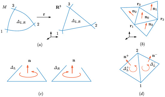
Figure 2. (a) A mapping $\mathbf{r}$ from a smooth triangle in M to a piecewise linear triangle in ${\mathbf{R}}^3$; (b) a triangle and the three neighboring triangles in ${\mathbf{R}}^3$; (c) the definition of $\mathbf{n}$ on the triangles $\Delta$${}_{L,R}$; and (d) two neighboring triangles $\Delta$${}_L^{\pm }$ with unit normal vectors ${\mathbf{n}}^{\pm }$ and their common bond 12. The suffices of $\Delta$${}_{L,R}$ denote the orientation of the triangle. The open circles with an arrow at one terminal point indicate the surface orientation.

The surface inversion is given by:

$${\mathbf{r}}_i\to -{\mathbf{r}}_i\left(\mathrm{for}\mathrm{all}i\right),$$

(2)

for example. The problem is whether the inverted surface is stable or not. As we will see below, the energy of the inverted surface is different from that of the original surface in a non-Euclidean metric model. This non-Euclidean metric model becomes well-defined if it is treated as an FG model. In the FG modeling (not in the standard HP modeling), we assume that the surface is locally invertible as in Figure 1d, which can be defined by the change of local coordinate orientation. Thus, studies on the stability of inverted surfaces become feasible within the scope of FG modeling, although the transformation of variables ${\mathbf{r}}_i$ for this local inversion is not always given by Equation (2); the vertex position remains unchanged under the change of triangle orientation.

3.2. Discretization of the Model

In this subsection, the discretization of the Hamiltonian in Equation (1) is performed on the triangles $\Delta$${}_L$ and their image triangles $\mathbf{r}\left({\Delta }_L\right)$. The function $\rho$ in $g_{ab}$ is defined on each triangle $\Delta$ in M in the discrete model, and we denote the function $\rho$ on $\Delta$ by ${\rho }_{\Delta }$. Thus, the discrete metric defined on triangle $\Delta$ is given by:

$$g_{ab}=\left(\begin{array}{cc}1/{\rho }_{\Delta }& 0\\ 0& {\rho }_{\Delta }\end{array}\right),{\rho }_{\Delta }>0,\left(\mathrm{on}{\Delta }_L\right).$$

(3)

By replacing the integral and partial derivatives in $S_1$ and $S_2$ with the sum over triangles $\Delta$ and differences, respectively, such that:

$$\begin{array}{c}\hfill \begin{array}{c}\int \sqrt{g}{d}^{2}x\to \sum _{\Delta },\hfill \\ \frac{\partial \mathbf{r}}{\partial x_1}\to {\mathbf{r}}_2-{\mathbf{r}}_1,\frac{\partial \mathbf{r}}{\partial x_2}\to {\mathbf{r}}_3-{\mathbf{r}}_1,\hfill \\ \frac{\partial \mathbf{n}}{\partial x_1}\to {\mathbf{n}}_0-{\mathbf{n}}_2,\frac{\partial \mathbf{n}}{\partial x_2}\to {\mathbf{n}}_0-{\mathbf{n}}_3,\hfill \end{array}\end{array}$$

(4)

we have the discrete expressions $g^{11}{({\mathbf{r}}_2-{\mathbf{r}}_1)}^2+g^{22}{({\mathbf{r}}_3-{\mathbf{r}}_1)}^2$ and $g^{11}{({\mathbf{n}}_0-{\mathbf{n}}_2)}^2+g^{22}{({\mathbf{n}}_0-{\mathbf{n}}_3)}^2$ corresponding to the discrete energies $g^{ij}(\partial \mathbf{r}/\partial x_i)·(\partial \mathbf{r}/\partial x_j)$ and $g^{ij}(\partial \mathbf{n}/\partial x_i)·(\partial \mathbf{n}/\partial x_j)$ of $S_1$ and $S_2$ on triangle $\Delta$, where the local coordinate origin is assumed at Vertex 1 (see Figure 2b). Thus, the corresponding discrete expressions of $S_1$ and $S_2$ are given by:

$$\begin{array}{c}\hfill \begin{array}{c}{S}_1=\sum _{\Delta }{S}_1\left(\Delta \right)=\sum _{\Delta }\left(\rho {\ell }_{12}^2+\frac{1}{\rho }{\ell }_{13}^2\right),\hfill \\ S_2=\sum _{\Delta }{S}_2\left(\Delta \right)=\sum _{\Delta }\left[\rho \left(1-{\mathbf{n}}_0·{\mathbf{n}}_2\right)+\frac{1}{\rho }\left(1-{\mathbf{n}}_0·{\mathbf{n}}_3\right)\right],\hfill \end{array}\end{array}$$

(5)

where ${\ell }_{ij}=|{\overrightarrow{\ell }}_{ij}|=|{\mathbf{r}}_j-{\mathbf{r}}_i|$. The index i of ${\mathbf{n}}_i$ in this $S_2$ represents a triangle (see Figure 2b). Since the coordinate origin can also be assumed at Vertices 2 and 3 on triangle $\Delta$, we have three possible discrete expressions, including those in Equation (5) for $g^{ij}(\partial \mathbf{r}/\partial x_i)·(\partial \mathbf{r}/\partial x_j)$ and $g^{ij}(\partial \mathbf{n}/\partial x_i)·(\partial \mathbf{n}/\partial x_j)$. Thus, we have:

$$\begin{array}{c}\hfill \begin{array}{c}{S}_1=\frac{1}{3}\sum _{\Delta }\left[\left({\rho }_1+\frac{1}{{\rho }_2}\right){\ell }_{12}^2+\left({\rho }_2+\frac{1}{{\rho }_3}\right){\ell }_{23}^2+\left({\rho }_3+\frac{1}{{\rho }_1}\right){\ell }_{31}^2\right],\hfill \\ S_2=\frac{1}{3}\sum _{\Delta }\left[\left({\rho }_2+\frac{1}{{\rho }_1}\right)\left(1-{\mathbf{n}}_0·{\mathbf{n}}_3\right)+\left({\rho }_3+\frac{1}{{\rho }_2}\right)\left(1-{\mathbf{n}}_0·{\mathbf{n}}_1\right)\right.\hfill \\ +\left.\left({\rho }_1+\frac{1}{{\rho }_3}\right)\left(1-{\mathbf{n}}_0·{\mathbf{n}}_2\right)\right],\hfill \end{array}\end{array}$$

(6)

where the factor $1/3$ is assumed. In the expressions, the suffix i of ${\rho }_i$ denotes the coordinate origin. The reason why the function $\rho$ depends on the coordinate origin is that $\rho$ is an element of $2\times 2$ matrix $g_{ab}$, which depends on local coordinates in general.

The expressions for $S_1$ and $S_2$ in Equations (5) and (6) correspond to those for $\Delta$${}_L$. In Equation (6), the sum over triangles ${\sum }_{\Delta }$ in $S_1$ and $S_2$ can be replaced by sum over bonds ${\sum }_{ij}$. In this replacement, we should remind ourselves of the fact that the first terms of $S_1$ and $S_2$ in (6) are respectively replaced by $\left({\rho }_1^{+}+1/{\rho }_2^{+}+{\rho }_2^{-}+1/{\rho }_1^{-}\right){\ell }_{12}^2$ and $\left({\rho }_2^{+}+1/{\rho }_1^{+}+{\rho }_1^{-}+1/{\rho }_2^{-}\right)\left(1-{\mathbf{n}}^{+}·{\mathbf{n}}^{-}\right)$. In these expressions, ${\rho }_i^{\pm }$ denotes the function $\rho$ on the triangles $\Delta$${}_L^{\pm }$, where the coordinate origin is at vertex i (see Figure 2d), and ${\mathbf{n}}^{\pm }$ denote $\mathbf{n}$ for triangles $\Delta$${}_L^{\pm }$. The coefficient of ${\ell }_{12}^2$ is different from that of $\left(1-{\mathbf{n}}^{+}·{\mathbf{n}}^{-}\right)$, and these coefficients come from the following expressions:

$$\begin{array}{c}\hfill \begin{array}{c}{S}_1\left({\Delta }_L^{+}\right)=\left({\rho }_1^{+}+1/{\rho }_2^{+}\right){\ell }_{12}^2+\cdots ,\hfill \\ S_1\left({\Delta }_L^{-}\right)=\left({\rho }_2^{-}+1/{\rho }_1^{-}\right){\ell }_{12}^2+\cdots ,\hfill \\ S_2\left({\Delta }_L^{+}\right)=\left({\rho }_2^{+}+1/{\rho }_1^{+}\right)\left(1-{\mathbf{n}}^{+}·{\mathbf{n}}^{-}\right)+\cdots ,\hfill \\ S_2\left({\Delta }_L^{-}\right)=\left({\rho }_1^{-}+1/{\rho }_2^{-}\right)\left(1-{\mathbf{n}}^{+}·{\mathbf{n}}^{-}\right)+\cdots .\hfill \end{array}\end{array}$$

(7)

Thus, we have:

$$\begin{array}{c}\hfill \begin{array}{c}{S}_1=\sum _{ij}{\gamma }_{ij}{\ell }_{ij}^2,S_2=\sum _{ij}{\kappa }_{ij}\left(1-{\mathbf{n}}^{+}·{\mathbf{n}}^{-}\right),\hfill \\ {\gamma }_{ij}=\left({\gamma }_{ij}^{+}+{\gamma }_{ij}^{-}\right)/4,{\kappa }_{ij}=\left({\kappa }_{ij}^{+}+{\kappa }_{ij}^{-}\right)/4,\hfill \\ {\gamma }_{ij}^{+}={\rho }_i^{+}+1/{\rho }_j^{+},{\kappa }_{ij}^{+}={\rho }_j^{+}+1/{\rho }_i^{+},\left(\mathrm{on}{\Delta }_L^{+}\right),\hfill \\ {\gamma }_{ij}^{-}={\rho }_j^{-}+1/{\rho }_i^{-},{\kappa }_{ij}^{-}={\rho }_i^{-}+1/{\rho }_j^{-},\left(\mathrm{on}{\Delta }_L^{-}\right),\hfill \end{array}\end{array}$$

(8)

where the factor $1/3$ is replaced by $1/4$ in the final expressions of $S_1$ and $S_2$. The indices $ij$ of ${\gamma }_{ij}$ and ${\kappa }_{ij}$ simply denote vertices i and j. We should note that ${\gamma }_{ij}={\kappa }_{ji}$ and ${\gamma }_{ij}\ne {\kappa }_{ij}$ in general in Equation (8), as mentioned above.

The partition function Z and Hamiltonian S of the model we start with in this paper are defined by:

$$\begin{array}{c}\hfill \begin{array}{c}Z(\lambda ,\kappa )=\sum _{\sigma }\sum _{\mathcal{T}}{\int }^{\prime }\prod _{i=1}^{N}d{\mathbf{r}}_{i}exp\left[-S(\mathbf{r},\sigma )\right],\hfill \\ S=\lambda S_0+S_1+\kappa S_2,S_0=\sum _{\pm }\left(1-{\sigma }^{+}·{\sigma }^{-}\right),\left({\sigma }^{\pm }\in \{1,-1\}\right),\hfill \end{array}\end{array}$$

(9)

where Ising model energy $S_0$ with the coefficient $\lambda$ is included in S. This is a surface model for multi-component membranes [13]. The sum ${\sum }_{\pm }$ in $S_0$ denotes the sum over all nearest neighbor triangles + and −, and ${\sigma }^{\pm }$ denotes that $\sigma$ is defined on the triangles $\Delta$${}_L^{\pm }$. The variable $\sigma$ is an element of ${\mathbf{Z}}_2=\{1,-1\}$; however, $S_0$ (and $\sigma$) is not always limited to the Ising-type Hamiltonian. The variable ${\sigma }^{\pm }$ is introduced to represent the components A and B, such as liquid-ordered and liquid-disordered phases [13]. If ${\sigma }^{+}=1(-1)$ on triangle $\Delta$${}^{+}$, this triangle $\Delta$${}^{+}$ is understood such that it belongs to or is occupied by the component A (B) for example. The value of $\sigma$ on each triangle $\Delta$ remains unchanged; however, the energy $S_0$ does not remain constant because the combination of nearest neighbor pairs of triangles $\Delta$${}^{\pm }$ changes due to the triangle diffusion, which is actually expected on dynamically-triangulated surfaces [13]. In the model of [13], the function ${\rho }_i^{+}$ is independent of vertex i and depends only on triangle $\Delta$${}^{+}$, and therefore, the value of ${\rho }^{+}$ is uniquely determined only by ${\sigma }^{+}$ if the dependence of ${\rho }^{+}$ on ${\sigma }^{+}$ is fixed. As a consequence, the metric $g_{ab}$ is determined by the internal variable $\sigma$. In the model of Equation (9), the dependence of ${\rho }_i^{+}$ on ${\sigma }^{+}$ is not explicitly specified, because this dependence of $\rho$ on $\sigma$ is in general independent of the well definedness of discrete surface models with non-Euclidean metric, and this well definedness is the main target in this paper.

In Z, ${\sum }_{\sigma }$ and ${\sum }_{\mathcal{T}}$ denote the sum over all possible configurations of $\sigma$ and triangulations $\mathcal{T}$, respectively. The sum over triangulation ${\sum }_{\mathcal{T}}$ can be simulated by the bond flips in MC simulations, and therefore, the model is grouped into the fluid surface models as mentioned in the Introduction. The symbol $\mathcal{T}$ in ${\sum }_{\mathcal{T}}$ denotes the triangulation, which is assumed as one of the dynamical variables of the discrete fluid model. This means that a variable $\mathcal{T}$ corresponds to a triangulated lattice configuration. Therefore, the lattice configurations in the parameter space M are determined by $\mathcal{T}$. On the other hand, a lattice configuration corresponding to a given $\mathcal{T}$ is originally considered as an ingredient of a set of local coordinate systems; two different $\mathcal{T}$’s correspond to two inequivalent coordinates, which are not transformed to each other by any coordinate transformation. Recalling that the continuous Hamiltonian is invariant under general coordinated transformations, we can chose an arbitrary coordinate, such as the orthogonal coordinate for each triangle of a given $\mathcal{T}$. However, from Polyakov’s string theoretical point of view, the partition function is defined by the sum over all possible metrices $\int \mathcal{D}g$ in addition to the sum over all possible mappings $\int \mathcal{D}\mathbf{r}$. Since the metric g depends on coordinates, $\int \mathcal{D}g$ is considered to be corresponding to the sum over local coordinates, which is simulated by ${\sum }_{\mathcal{T}}$ in the discrete models. Therefore, from these intuitive discussions, the Euclidean metric, for example, is forbidden in a fluid model on triangulated lattices without DT; this Euclidean metric model without DT is simply an FC model for polymerized membranes, where the surface inversion is not expected.

The symbol ${\int }^{\prime }{\prod }_{i=1}^{N}d{\mathbf{r}}_i$ denotes $3(N-1)$-dimensional integrations in ${\mathbf{R}}^3$ under the condition that the center of mass of the surface is fixed to the origin of ${\mathbf{R}}^3$. The Hamiltonian S has the unit of energy $\left[k_{B}T\right]$. The coefficient $\kappa \left[k_{B}T\right]$ of $S_2$ is the bending rigidity.

Here, we comment on the property called scale invariance of the model [35]. This comes from the fact that the integration of $\mathbf{r}$ in Z is independent of the scale transformation, such that $\mathbf{r}\to \alpha \mathbf{r}$ for arbitrary positive $\alpha \in \mathbf{R}$. This property is expressed by $Z\left(\right\{\mathbf{r}\left\}\right)=Z\left(\right\{\alpha \mathbf{r}\left\}\right)$, and therefore, for Hamiltonian $S^{\prime }=\lambda S_0+c{S}_1+\kappa S_2$, we have:

$$\begin{array}{c}\hfill \begin{array}{cc}& \sum _{\sigma }\sum _{\mathcal{T}}{\int }^{\prime }\prod _{i=1}^{N}d{\mathbf{r}}_{i}exp\left[-S^{\prime }\left(\mathbf{r}\right)\right]\hfill \\ \hfill =& {\alpha }^{3N-1}\sum _{\sigma }\sum _{\mathcal{T}}{\int }^{\prime }\prod _{i=1}^{N}d{\mathbf{r}}_{i}exp\left[-\left(\lambda S_0+c{\alpha }^2{S}_1+\kappa S_2\right)\right]\hfill \\ \hfill =& c^{-(3N-1)/2}\sum _{\sigma }\sum _{\mathcal{T}}{\int }^{\prime }\prod _{i=1}^{N}d{\mathbf{r}}_{i}exp\left[-\left(\lambda S_0+S_1+\kappa S_2\right)\right]\hfill \\ \hfill =& c^{-(3N-1)/2}\sum _{\sigma }\sum _{\mathcal{T}}{\int }^{\prime }\prod _{i=1}^{N}d{\mathbf{r}}_{i}exp\left[-S\left(\mathbf{r}\right)\right].\hfill \end{array}\end{array}$$

(10)

In the second line of Equation (10), we assume $\alpha =1/\sqrt{c}$, and then in the third line, we have $S^{\prime }\left(\alpha \mathbf{r}\right)=\lambda S_0+S_1+\kappa S_2$ because $S_0$ and $S_2$ are scale independent and $S_1\left(\alpha \mathbf{r}\right)={\alpha }^2{S}_1\left(\mathbf{r}\right)$. Thus, from the fact that the partition function is independent of the multiplicative constant, we find that the model with $S^{\prime }=\lambda S_0+c{S}_1+\kappa S_2$ is equivalent to the model with $S=\lambda S_0+S_1+\kappa S_2$. “Equivalent” means that the shape of the surface is independent of the value of $c(>0)$, although the surface size depends on c in general. The dependence of surface size on c is also understood from the scale-invariant property of Z. Indeed, it follows from $Z\left(\right\{\mathbf{r}\left\}\right)=Z\left(\right\{\alpha \mathbf{r}\left\}\right)$ that ${\partial Z\left(\left\{\alpha \mathbf{r}\right\}\right)/\partial \alpha |}_{\alpha =1}=0$, and therefore, we have [35]:

$$\begin{array}{c}\hfill \begin{array}{cc}& {\left.\frac{\partial logZ\left[S^{\prime }\left(\alpha \mathbf{r}\right)\right]}{\partial \alpha }\right|}_{\alpha =1}\hfill \\ \hfill =& \frac{1}{Z}{\left[(3N-1){\alpha }^{3N-2}Z-2c{\alpha }^{3N}\sum _{\sigma }\sum _{\mathcal{T}}{\int }^{\prime }\prod _{i=1}^{N}d{\mathbf{r}}_i{S}_{1}exp\left[-\left(\lambda S_0+c{\alpha }^2{S}_1+\kappa S_2\right)\right]\right]}_{\alpha =1}\hfill \\ \hfill =& (3N-1)-2c⟨S_1⟩=0\iff ⟨S_1⟩/N=3/\left(2c\right).\hfill \end{array}\end{array}$$

(11)

This final equation implies that the mean bond length squares $⟨{\ell }_{ij}^2⟩$ depends on c, because $S_1$ is given by $S_1={\sum }_{ij}{\gamma }_{ij}{\ell }_{ij}^2$ where ${\gamma }_{ij}$ is independent of c. For a specialized case that ${\gamma }_{ij}$ = constant, $⟨S_1⟩$ becomes proportional to $⟨{\ell }_{ij}^2⟩$. On the other hand, the mean bond length squares in general represent the surface size for smooth surfaces, which are expected for sufficiently large $\kappa$.

We should note that the model studied in [13] for a two-component membrane is obtained from the model of Equations (8) and (9) by the assumption that ${\rho }_i^{\pm }$ is independent of the local coordinate origin i and depends only on triangles $\Delta$${}^{\pm }$. In this case, the model is orientation symmetric, and therefore, the lower suffices $L,R$ for the orientation of triangles $\Delta$${}_{L,R}$ are not necessary. Then, we have ${\gamma }_{ij}={\kappa }_{ij}=(1/4)\left({\rho }^{+}+1/{\rho }^{+}+{\rho }^{-}+1/{\rho }^{-}\right)$, where + and − are the two neighboring triangles of bond $ij$, which links vertices i and j. Thus, ${\gamma }_{ij}$ (and ${\kappa }_{ij}$) defined on bond $ij$ depends only on ${\rho }^{\pm }$ of the two neighboring triangles in the model of [13]. For this reason, the configuration (or distribution) of $\rho$ on the surface remains unchanged if the triangulation is fixed. However, the model is defined on dynamically-triangulated lattices, which allow not only vertices, but also triangles to diffuse freely over the surface [22,23,24]. This free diffusion of triangles changes the distribution of $\rho$ and, hence, ${\gamma }_{ij}$ and ${\kappa }_{ij}$. Moreover, $\sigma (\in {\mathbf{Z}}_2)$ is assigned on triangles (not on vertices) such that the value of ${\rho }^{\pm }$ on each triangle is determined by ${\sigma }^{\pm }(\in {\mathbf{Z}}_2)$. As a consequence, the corresponding energy $S_0={\sum }_{\pm }\left(1-{\sigma }^{+}·{\sigma }^{-}\right)$ becomes dependent on the distribution of $\rho$ or, in other words, the distribution of ${\gamma }_{ij}$ and ${\kappa }_{ij}$ is determined by the energy $S_0$. This is an outline of the model in [13].

In this paper, ${\rho }_i^{\pm }$ depends on not only triangles $\Delta$${}^{\pm }$, but also the local coordinate origin i in contrast to that of the model in [13]. We should note that the relation between ${\rho }^{\pm }$ and ${\sigma }^{\pm }$ is not explicitly specified. Although the model is not determined without the explicit relation, the following discussions in this paper are independent of this relation.

3.3. Well-Defined Model

We start with the definition of the trivial (non-trivial) model for a discrete surface model.

Definition 1.

Let us assume that Hamiltonian S of a discrete surface model is given by Equation (8). Then, this discrete model is called trivial (non-trivial) if the following conditions are (not) satisfied:

$$\begin{array}{c}\hfill {\gamma }_{ij}=\mathrm{constant},{\kappa }_{ij}=\mathrm{constant},\end{array}$$

(12)

where the constants are independent of bond $ij$, and these constants are not necessarily the same.

We assume $\lambda =0$ in S of Equation (8) for simplicity. We should note that a model with $S^{\prime }=c_1{S}_1+\kappa c_2{S}_2$, for arbitrary coefficients $c_1$ and $c_2$, is identical to the model defined by $S=S_1+{\kappa }^{\prime }{S}_2$ with ${\kappa }^{\prime }=\kappa c_2$. Indeed, because of the scale invariance of Z discussed in the previous subsection using Equation (10), the coefficient $c_1$ of $S_1$ in $S^{\prime }$ can be replaced by one. Thus, we have $S^{\prime }=S_1+{\kappa }^{\prime }{S}_2$.

If the metric is conformally equivalent to the Euclidean metric, then the model is trivial. In this sense, this definition for the trivial (non-trivial) model is an extension of the definition by the terminology conformally equivalent for $g_{ab}$ discussed in Section 3.1. However, there exists a metric that is conformally non-equivalent to ${\delta }_{ab}$ while it makes the model trivial. An example of such a metric is $g_{ab}=\left(\begin{array}{cc}2/(3+\sqrt{5})& 0\\ 0& (3+\sqrt{5})/2\end{array}\right)$, and more detailed information will be given below (in Remark 2).

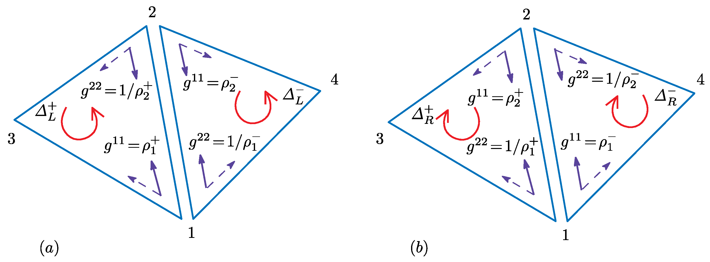
Next, we introduce the notion of direction-dependent length $L_{ij}$ (and $L_{ji}$) of bond $ij$, which is shared by two triangles, in the discrete model. Let $\Delta$${}_L^{\pm }$ be the two nearest neighbor triangles of Bond 12 on M (Figure 3a). The length $L_{12}\left({\Delta }_L^{+}\right)$ of Bond 12 is defined by $L_{12}\left({\Delta }_L^{+}\right)=\int d{x}_{1}1/{\rho }_1^{+}=1/{\rho }_1^{+}$, where $1/{\rho }_1^{+}$ is the element $g_{11}$ of the metric $g_{ab}$ on $\Delta$${}_L^{+}$ where the local coordinate origin is at Vertex 1; the symbol $\Delta$${}_L^{+}$ in $L_{12}\left({\Delta }_L^{+}\right)$ denotes that $L_{12}$ is defined by $g_{ab}$ on triangle $\Delta$${}_L^{+}$. It is also possible to define $L_{12}\left({\Delta }_L^{+}\right)$ by $L_{12}\left({\Delta }_L^{+}\right)=\int d{x}_2\left({\rho }_2^{+}\right)={\rho }_2^{+}$, where ${\rho }_2^{+}$ is the element $g_{22}$ on $\Delta$${}_L^{+}$ where the local coordinate origin is at Vertex 2. Thus, $L_{12}\left({\Delta }_L^{+}\right)$ is defined by the mean value of these two lengths, and the length $L_{21}\left({\Delta }_L^{-}\right)$ of Bond 12 is also defined in exactly same manner. Then, we have:

$$\begin{array}{c}\hfill L_{12}\left({\Delta }_L^{+}\right)=(1/2)\left(1/{\rho }_1^{+}+{\rho }_2^{+}\right),L_{21}\left({\Delta }_L^{-}\right)=(1/2)\left(1/{\rho }_2^{-}+{\rho }_1^{-}\right).\end{array}$$

(13)

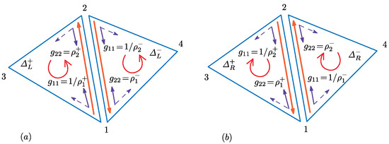
Figure 3. (a) Two neighboring triangles $\Delta$${}^{\pm }$ and elements of $g_{ab}$ for the direction dependent length of bond 12 at the vertices 1 and 2; and (b) the inverted triangles $\Delta$${}_R^{\pm }$ (inside view) of $\Delta$${}_L^{\pm }$ in (a). The direction dependent lengths of bond 12 are indicated by long arrows in both $\Delta$${}_L^{\pm }$ and $\Delta$${}_R^{\pm }$.

These two lengths are different from each other in their expressions, and therefore, it appears that the bond length is dependent on its direction. For the inverted surface (shown in Figure 3b), we also have the two different lengths:

$$\begin{array}{c}\hfill {\overline{L}}_{12}\left({\Delta }_R^{-}\right)=(1/2)\left(1/{\rho }_1^{-}+{\rho }_2^{-}\right),{\overline{L}}_{21}\left({\Delta }_R^{+}\right)=(1/2)\left(1/{\rho }_2^{+}+{\rho }_1^{+}\right).\end{array}$$

(14)

It is also possible to define the lengths of Bond 12 as follows:

$$\begin{array}{c}\hfill \begin{array}{c}{L}_{12}^{\prime }\left({\Delta }_L\right)=(1/2)\left(1/{\rho }_1^{+}+{\rho }_1^{-}\right),L_{21}^{\prime }\left({\Delta }_L\right)=(1/2)\left({\rho }_2^{+}+1/{\rho }_2^{-}\right),\hfill \\ {\overline{L}}_{12}^{\prime }\left({\Delta }_R\right)=(1/2)\left({\rho }_1^{+}+1/{\rho }_1^{-}\right),{\overline{L}}_{21}^{\prime }\left({\Delta }_R\right)=(1/2)\left(1/{\rho }_2^{+}+{\rho }_2^{-}\right),\hfill \end{array}\end{array}$$

(15)

where $L_{12}^{\prime }$ and $L_{21}^{\prime }$ (${\overline{L}}_{12}^{\prime }$ and ${\overline{L}}_{21}^{\prime }$) correspond to those in Equation (13) (Equation (14)). The following discussions remain unchanged if $L_{12}^{\prime }$, $L_{21}^{\prime }$ and ${\overline{L}}_{12}^{\prime }$, ${\overline{L}}_{21}^{\prime }$ are assumed as the definition of bond lengths. For this reason, we use only the expressions in Equation (13) and Equation (14) for bond lengths in the discussions below.

Now, let us introduce the notion of a well-defined model.

Definition 2.

A discrete surface model is called well defined if the following conditions are satisfied:

(A1)

Any bond length is independent of its direction

(A2)

Any bond length is independent of surface orientation

(A3)

Any triangle area is independent of surface orientation

We should note that these constraints (A1)–(A3) are not imposed on Finsler geometry models, which will be introduced in the following section. Using Equations (13) and (14), we rewrite the first and second conditions (A1) and (A2) such that:

$$\begin{array}{cc}\hfill & 1/{\rho }_1^{+}+{\rho }_2^{+}=1/{\rho }_2^{-}+{\rho }_1^{-},(\iff \left(\mathrm{A}1\right)),\hfill \end{array}$$

(16)

$$\begin{array}{cc}\hfill & 1/{\rho }_2^{-}+{\rho }_1^{-}=1/{\rho }_1^{-}+{\rho }_2^{-},1/{\rho }_1^{+}+{\rho }_2^{+}=1/{\rho }_2^{+}+{\rho }_1^{+}(\iff \left(\mathrm{A}2\right)).\hfill \end{array}$$

(17)

The condition (A3) is always satisfied because of the fact that $det{g}_{ab}=1$ for the metric function in Equation (3). Note that the constraint (A1) is imposed only on triangles ${\Delta }_L$, and the equation corresponding to (A1) on triangles ${\Delta }_R$ is not independent of the three equations in Equations (16) and (17).

If we use the following definition for the bond length consistency for every vertex:

$$\begin{array}{cc}\hfill & {\rho }_1^{-}=1/{\rho }_1^{+},(\iff \left(\mathrm{A}1\right)),\hfill \end{array}$$

(18)

$$\begin{array}{cc}\hfill & 1/{\rho }_1^{+}={\rho }_1^{+},{\rho }_1^{-}=1/{\rho }_1^{-}(\iff \left(\mathrm{A}2\right)),\hfill \end{array}$$

(19)

then we have ${\rho }_1^{+}={\rho }_1^{-}=1$ (Vertex 1 for simplicity). In this case, we have a trivial model because $g_{ab}={\delta }_{ab}$.

The discrete expression of the induced metric $g_{ab}={\partial }_a\mathbf{r}·{\partial }_b\mathbf{r}$ is given by $g_{ab}=\left(\begin{array}{cc}{\ell }_{12}^2& {\overrightarrow{\ell }}_{12}·{\overrightarrow{\ell }}_{13}\\ {\overrightarrow{\ell }}_{12}·{\overrightarrow{\ell }}_{13}& {\ell }_{13}^2\end{array}\right)$, which is defined on Triangle 123 in ${\mathbf{R}}^3$ with the local coordinate origin at ${\mathbf{r}}_1$ (see Figure 2b). This $g_{ab}$ is not of the form $\left(\begin{array}{cc}\hfill E& \hfill 0\\ \hfill 0& \hfill G\end{array}\right)$, and for this reason, the induced metric model is out of the scope of Definition 1. However, it is easy to see that the induced metric model satisfies (A1)–(A3) in Definition 2. Indeed, the bond length of this model is just the Euclidean length of Bond 12 in ${\mathbf{R}}^3$. Other conditions are also easy to confirm.

3.4. Orientation Symmetric Model

The discrete model is defined by the Hamiltonian in Equation (8), where $g_{ab}$ is a coordinate-dependent metric. Therefore, the Hamiltonian depends on the local coordinates on M, and it also depends on the orientation of M. For this reason, we define the notion of the orientation symmetric/asymmetric model defined on surfaces with $\Delta$${}_L$. This simply means that the Hamiltonian of Equation (8) can be used for a model in which the partition function allows the surface inversion process. Indeed, a property of the model corresponding to symmetries in Hamiltonian can be discussed without referencing the partition function in general. Thus, the Hamiltonian is called orientation symmetric if it is invariant under the surface inversion in Equation (2), for example for any configuration of $\mathbf{r}$, and we also have:

Definition 3.

A discrete surface model is called orientation symmetric if the Hamiltonian is orientation symmetric.

In the Hamiltonian of Equation (8), the quantities ${\gamma }_{ij}$ and ${\kappa }_{ij}$ in $S_1$ and $S_2$ depend on the surface orientation. Thus, the condition for that the Hamiltonian is orientation symmetric is as follows:

$$\begin{array}{cc}\hfill & 1/{\rho }_1^{-}+{\rho }_2^{-}+1/{\rho }_2^{+}+{\rho }_1^{+}=1/{\rho }_2^{-}+{\rho }_1^{-}+1/{\rho }_1^{+}+{\rho }_2^{+}\hfill \end{array}$$

(20)

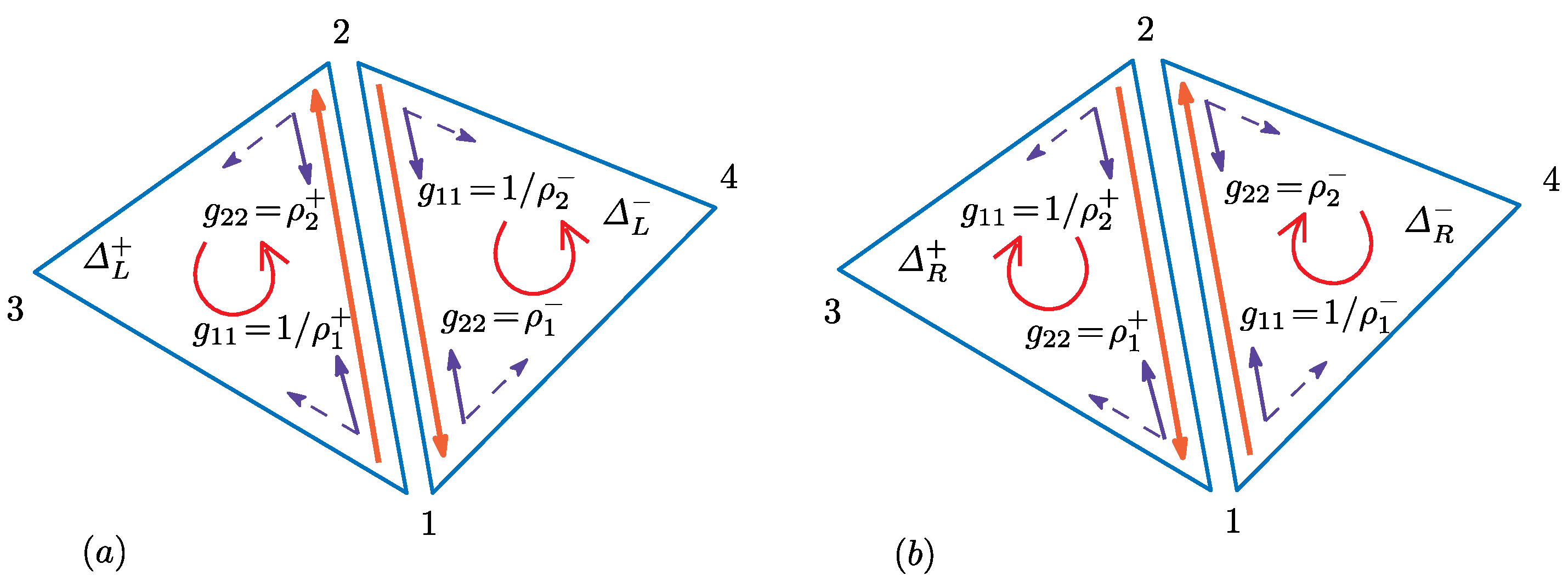
for all bonds 12 and $\Delta$${}^{\pm }$. Indeed, the Gaussian bond potential $S_1\left({\ell }_{12}\right)$ of Bond 12 is given by $S_1\left({\ell }_{12}\right)=(1/4)\left(1/{\rho }_1^{-}+{\rho }_2^{-}+1/{\rho }_2^{+}+{\rho }_1^{+}\right){\ell }_{12}^2$ (Figure 4a), while on the inverted triangles, the corresponding quantity ${\overline{S}}_1\left({\ell }_{12}\right)$ is given by ${\overline{S}}_1\left({\ell }_{12}\right)=(1/4)\left(1/{\rho }_2^{-}+{\rho }_1^{-}+1/{\rho }_1^{+}+{\rho }_2^{+}\right){\ell }_{12}^2$. These $S_1\left({\ell }_{12}\right)$ and ${\overline{S}}_1\left({\ell }_{12}\right)$ are obtained by using the following expression for the inverse metric:

$$g^{ab}=g_{ab}^{-1}=\left(\begin{array}{cc}\rho & 0\\ 0& 1/\rho \end{array}\right).$$

(21)

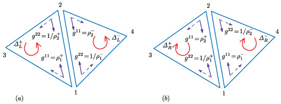
Figure 4. (a) Two neighboring triangles $\Delta$${}_L^{\pm }$ and elements of the inverse metric $g^{ab}$ for $S_1$ and $S_2$; and (b) the inverted triangles $\Delta$${}_R^{\pm }$ (inside view).

Thus, from the equation $S_1\left({\ell }_{12}\right)={\overline{S}}_1\left({\ell }_{12}\right)$ for any Bond 12, which is the condition for $S_1$ to be orientation symmetric, we have Equation (20). We should note that from the condition $S_2({\mathbf{n}}^{+}·{\mathbf{n}}^{-})={\overline{S}}_2({\mathbf{n}}^{+}·{\mathbf{n}}^{-})$ for the bending energy $S_2$, the same equation as Equation (20) is obtained.

Remark 1.

We have the following remarks:

(a)

All non-trivial models are orientation asymmetric

(b)

All orientation asymmetric models are ill-defined

Proof of Remark 1.

(a) The inverse metric $g^{ab}$ of a non-trivial model is given by Equation (21), and therefore, it is easy to see that there exists a bond 12, such that $S_1\left({\ell }_{12}\right)\ne {\overline{S}}_1\left({\ell }_{12}\right)$. Indeed, we can choose $\rho$’s such that Equation (20) is not satisfied. This inequality $S_1\left({\ell }_{12}\right)\ne {\overline{S}}_1\left({\ell }_{12}\right)$ implies that the condition in Equation (20) is not satisfied and that the model is orientation asymmetric. (b) ⇔ All well-defined models are orientation symmetric, which can be proven as follows: if the model is well-defined, then Equations (16) and (17) are satisfied. Then, it is easy to see that Equation (20) is satisfied. This implies that the model is orientation symmetric. ☐

From Remark 1, it is straightforward to prove the following theorem:

Theorem 1.

All non-trivial models are ill-defined.

Here, we should clarify how well-defined models are different from the model with Euclidean metric ${\delta }_{ab}$. This problem is rephrased such that what type of $\rho$ is allowed for a well-defined model. The answer is as follows:

Remark 2.

We have the following remarks:

(a)

The function ${\rho }_i$ of any well-defined model satisfies:

$$\begin{array}{c}\hfill 1/{\rho }_i+{\rho }_i=a(=\mathrm{const}),\end{array}$$

(22)

where the constant a depends on neither vertex i, nor triangle Δ.

(b)

There are two possible ρs, which are solutions of Equation(22):

$$\begin{array}{c}\hfill {\rho }_{\pm }=\frac{1}{2}\left(a\pm \sqrt{a^2-4}\right)\end{array}$$

(23)

(c)

If Equation (22) is satisfied, then the model is trivial.

Proof of Remark 2.

(a) A well-defined model satisfies Equations (16) and (17). Multiplying both sides of the first equation in Equation (17) by ${\rho }_1^{-}{\rho }_2^{-}(>0)$, we have ${\rho }_1^{-}\left({\rho }_1^{-}{\rho }_2^{-}+1\right)={\rho }_2^{-}\left({\rho }_1^{-}{\rho }_2^{-}+1\right)$, and therefore, ${\rho }_1^{-}={\rho }_2^{-}(={\rho }^{-})$. It is also easy to see that ${\rho }_1^{+}={\rho }_2^{+}(={\rho }^{+})$ from the second equation in Equation (17). Therefore, using these two equations and Equation (16), we have ${\rho }_1^{-}+1/{\rho }_1^{-}={\rho }_1^{+}+1/{\rho }_1^{+}$. This implies that the combination ${\rho }^{-}+1/{\rho }^{-}$ is independent of the vertex and triangle, and thus, Equation (22) is proven. (b) It is easy to see that ${\rho }_{\pm }=\left(a\pm \sqrt{a^2-4}\right)/2$, ($a\ge 2$) from Equation (22). (c) Indeed, using Equation (22), we have ${\gamma }_{ij}={\kappa }_{ji}=(1/4)\left({\rho }^{+}+1/{\rho }^{+}+{\rho }^{-}+1/{\rho }^{-}\right)=a/2$, and therefore, $S_1\left(a\right)={\sum }_{ij}{\gamma }_{ij}{\ell }_{ij}^2=(a/2){\sum }_{ij}{\ell }_{ij}^2$ and $S_2\left(a\right)={\sum }_{ij}{\kappa }_{ij}\left(1-{\mathbf{n}}_i·{\mathbf{n}}_j\right)=(a/2){\sum }_{ij}\left(1-{\mathbf{n}}_i·{\mathbf{n}}_j\right)$. ☐

It follows from Remark 2(a) that the model in [13] is ill-defined (in the context of HP model). In fact, the metric function assumed in the model of [13] does not satisfy Equation (22). The metric corresponding to Remark 2(b) shows examples of metric for the trivial model, which is defined by Definition 1. More explicitly, $\left(\begin{array}{cc}1/{\rho }_{+}& 0\\ 0& {\rho }_{+}\end{array}\right)$ and $\left(\begin{array}{cc}1/{\rho }_{-}& 0\\ 0& {\rho }_{-}\end{array}\right)$ make the model trivial. The metrices $\left(\begin{array}{cc}1/{\rho }_{+}& 0\\ 0& {\rho }_{-}\end{array}\right)$ and $\left(\begin{array}{cc}1/{\rho }_{-}& 0\\ 0& {\rho }_{+}\end{array}\right)$ are conformally equivalent to ${\delta }_{ab}$, because ${\rho }_{+}{\rho }_{-}=1$, and therefore, these also make the model trivial. We should remark that Remarks 2(a) and 2(c) also prove Theorem 1.

Note also that if a model is well-defined and orientation symmetric in the sense of Definitions 2 and 3, then inverted triangles $\Delta$${}_R$ need not be included in the lattice configuration. However, from Theorem 1, the model introduced in Equation (8) is orientation asymmetric, and this model turns out to be well-defined if it is treated as an FG model. Therefore the inverted triangles $\Delta$${}_R$ should be included as a representation configuration of the model of Equation (8) if it is understood as a well-defined model. For this reason, we have to extend the FG model introduced in [15] such that the Hamiltonian has values on both $\Delta$${}_L$ and $\Delta$${}_R$.

4. Finsler Geometry Modeling

4.1. Finsler Geometry Model

As we have demonstrated in the previous subsection, all non-trivial surface models (⇔ either ${\gamma }_{ij}$ or ${\kappa }_{ij}$ depends on $ij$) are ill-defined. The reason why this unsatisfactory result is obtained is because the bond length should not be direction dependent for any well-defined models (see Definition 2). To make these ill-defined models meaningful, we introduce the notion of Finsler geometry, where length unit is allowed to be dependent on the direction. In the context of Finsler geometry modeling, Theorem 1 does not hold. The problem is whether or not the above mentioned ill-defined model (in Section 3) is fitted in Finsler geometry modeling.

Let $\Delta$${}_{L,R}$ be triangles in M and $x=(x_1,x_2)$ be a local coordinate on $\Delta$${}_{L,R}$, where the coordinate origin is at Vertex 1. Let $y=(y_1,y_2)$ be defined by $y_i=d{x}_i/dt,(i=1,2)$, where t is a parameter that increases toward the positive direction of the axes. It is also assumed that a positive parameter $v_{ij}$ is defined on the axis from vertex i to vertex j, where $v_{ij}\ne v_{ji}$ in general.

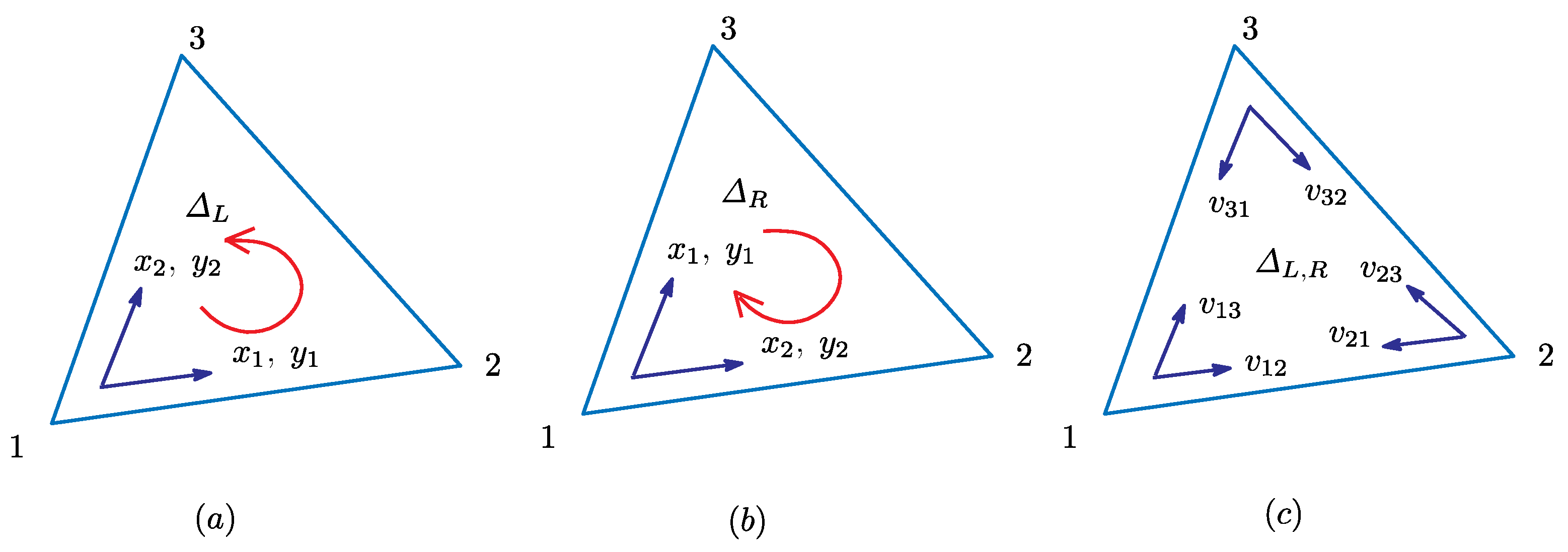
Discrete Finsler functions on triangles $\Delta$${}_{L,R}$ in M are defined by (Figure 5a,b):

$$\begin{array}{c}\hfill L_{{\Delta }_L}(x,y)=\left\{\begin{array}{cc}\hfill y_1/v_{12}& \hfill \left(\mathrm{on}{x}_1\mathrm{axis}\right)\\ \hfill y_2/v_{13}& \hfill \left(\mathrm{on}{x}_2\mathrm{axis}\right)\end{array}\right.,L_{{\Delta }_R}(x,y)=\left\{\begin{array}{cc}\hfill y_1/v_{13}& \hfill \left(\mathrm{on}{x}_1\mathrm{axis}\right)\\ \hfill y_2/v_{12}& \hfill \left(\mathrm{on}{x}_2\mathrm{axis}\right)\end{array}\right.,\end{array}$$

(24)

which can also be written as the bilinear forms:

$$\begin{array}{c}\hfill L_{{\Delta }_L}^2(x,y)=v_{12}^{-2}{y}_1^2+v_{13}^{-2}{y}_2^2,L_{{\Delta }_R}^2(x,y)=v_{13}^{-2}{y}_1^2+v_{12}^{-2}{y}_2^2.\end{array}$$

(25)

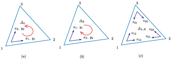
Figure 5. A triangle 123 with the local coordinate axis $x_i$ and the tangent vector component $y_i(={\dot{x}}_i)$ at Vertex 1 on the (a) left-handed triangle $\Delta$${}_L$ and (b) right-handed triangle $\Delta$${}_R$; and (c) three possible local coordinates on triangle $\Delta$${}_{L,R}$ and positive number $v_{ij}$ assigned along the bond $ij$.

From these expressions, we have the metric functions $g_{ab,L}$ on $\Delta$${}_L$ and $g_{ab,R}\left(x\right)$ on $\Delta$${}_R$, such that:

$$g_{ab,L}\left(x\right)=\frac{1}{2}\frac{\partial L_{{\Delta }_L}^2(x,y)}{\partial y_a\partial y_b}=\left(\begin{array}{cc}{v}_{12}^{-2}& 0\\ 0& v_{13}^{-2}\end{array}\right),g_{ab,R}\left(x\right)=\frac{1}{2}\frac{\partial L_{{\Delta }_R}^2(x,y)}{\partial y_a\partial y_b}=\left(\begin{array}{cc}{v}_{13}^{-2}& 0\\ 0& v_{12}^{-2}\end{array}\right).$$

(26)

In general, $g_{ab}$ is a function with respect to x and y; however, $g_{ab,LR}$ in Equation (26) only depends on the local coordinate x, and it is independent of y.

Using the metric $g_{ab,LR}$ in Equation (26) and summing over all possible coordinate origins on triangle $\Delta$${}_{L,R}$, just the same as in Equation (6), we have the discrete Hamiltonian such that (see Figure 2b):

$$\begin{array}{c}\hfill \begin{array}{c}{S}_1=\sum _{\Delta }\left({\gamma }_{12}{\ell }_{12}^2+{\gamma }_{23}{\ell }_{23}^2+{\gamma }_{31}{\ell }_{31}^2\right),\hfill \\ S_2=\sum _{\Delta }\left[{\kappa }_{12}\left(1-{\mathbf{n}}_0·{\mathbf{n}}_3\right)+{\kappa }_{23}\left(1-{\mathbf{n}}_0·{\mathbf{n}}_1\right)+{\kappa }_{31}\left(1-{\mathbf{n}}_0·{\mathbf{n}}_2\right)\right],\hfill \\ {\gamma }_{12}=\frac{v_{12}}{v_{13}}+\frac{v_{21}}{v_{23}},{\gamma }_{23}=\frac{v_{23}}{v_{21}}+\frac{v_{32}}{v_{31}},{\gamma }_{31}=\frac{v_{31}}{v_{32}}+\frac{v_{13}}{v_{12}},\hfill \\ {\kappa }_{12}=\frac{v_{13}}{v_{12}}+\frac{v_{23}}{v_{21}},{\kappa }_{23}=\frac{v_{21}}{v_{23}}+\frac{v_{31}}{v_{32}},{\kappa }_{31}=\frac{v_{32}}{v_{31}}+\frac{v_{12}}{v_{13}}.\hfill \end{array}\end{array}$$

(27)

The sum over triangles ${\sum }_{\Delta }$ in $S_1$ and $S_2$ can also be expressed by the sum over bonds with a numerical factor $1/4$. Thus, we have:

$$\begin{array}{c}\hfill \begin{array}{c}S=S_1+\kappa S_2,\hfill \\ S_1=\frac{1}{4}\sum _{ij}\left({\gamma }_{ij}^{+}+{\gamma }_{ij}^{-}\right){\ell }_{ij}^2,S_2=\frac{1}{4}\sum _{ij}\left({\kappa }_{ij}^{+}+{\kappa }_{ij}^{-}\right)\left(1-{\mathbf{n}}^{+}·{\mathbf{n}}^{-}\right),\hfill \\ {\gamma }_{12}^{+}=\frac{v_{12}}{v_{13}}+\frac{v_{21}}{v_{23}},{\gamma }_{12}^{-}=\frac{v_{12}}{v_{14}}+\frac{v_{21}}{v_{24}},{\kappa }_{12}^{+}=\frac{v_{13}}{v_{12}}+\frac{v_{23}}{v_{21}},{\kappa }_{12}^{-}=\frac{v_{14}}{v_{12}}+\frac{v_{24}}{v_{21}},\hfill \end{array}\end{array}$$

(28)

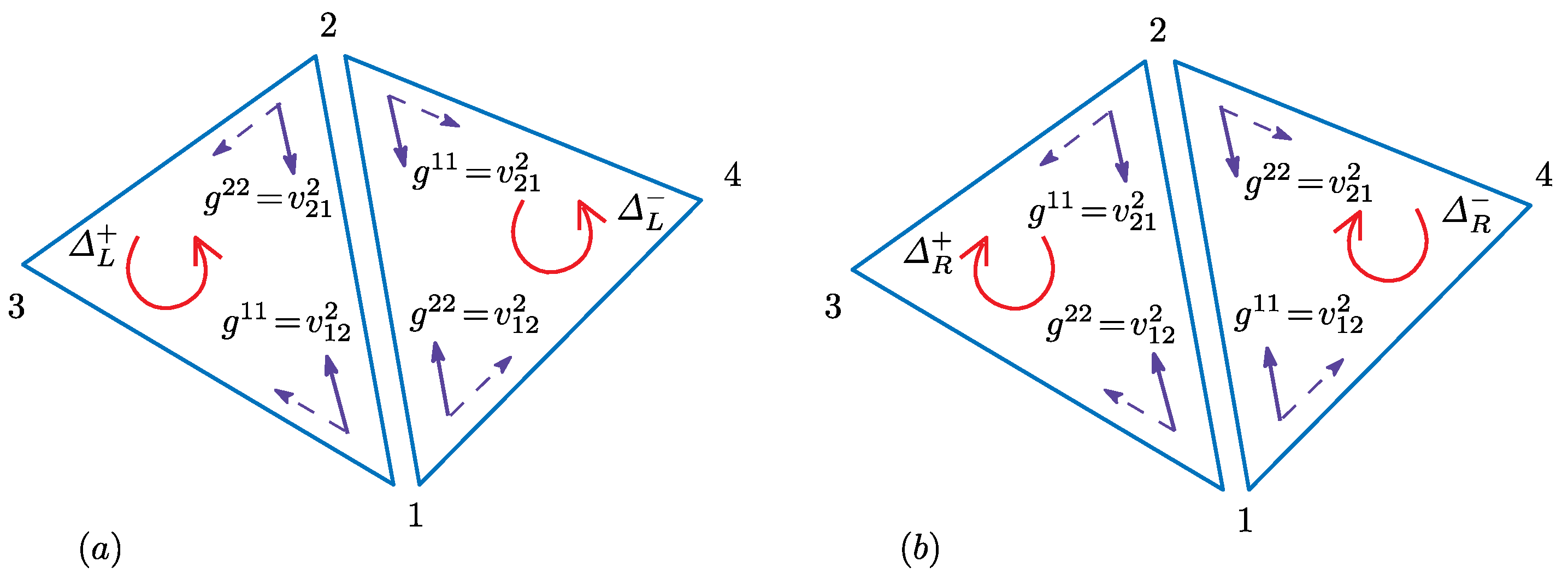
where ${\gamma }_{12}^{\pm }$ and ${\kappa }_{12}^{\pm }$ are concrete examples of ${\gamma }_{ij}^{\pm }$ and ${\kappa }_{ij}^{\pm }$ for Bond 12 (see Figure 5c). The symbol ± denotes that ${\gamma }_{ij}$ and ${\kappa }_{ij}$ are defined on the triangles $\Delta$${}_{L,R}^{\pm }$, which share the bond $ij$ (Figure 6a,b).

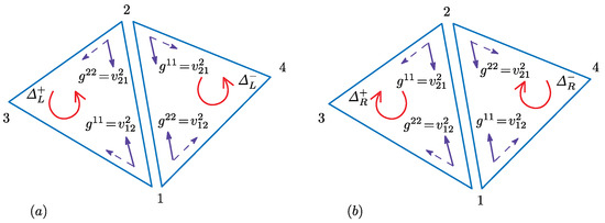
Figure 6. Two of four possible combinations of triangles $\Delta$${}_{L,R}^{+}$ and $\Delta$${}_{L,R}^{-}$, which share Bond 12: (a) $\Delta$${}_L^{+}$ and $\Delta$${}_L^{-}$ and (b) the inverted triangles $\Delta$${}_R^{+}$ and $\Delta$${}_R^{-}$ (inside view) of those in (a). Elements of the inverse metric $g^{ab}$ are given by $v_{12}^2$ and $v_{21}^2$, which are defined on Bond 12.

If the coefficients ${\gamma }_{ij}^{\pm }$ and ${\kappa }_{ij}^{\pm }$ are defined by the quantities, which are defined on vertices i and j or on bond $ij$, just like those in Equation (28), then these coefficients become independent of the orientation of the triangles. Therefore, we have ${\gamma }_{ij,L}^{\pm }={\gamma }_{ij,R}^{\pm }\left(={\gamma }_{ij}^{\pm }\right)$ and ${\kappa }_{ij,L}^{\pm }={\kappa }_{ij,R}^{\pm }\left(={\kappa }_{ij}^{\pm }\right)$, and therefore, the model is orientation symmetric. In this case, we have ${\gamma }_{ij}^{+}+{\gamma }_{ij}^{-}={\gamma }_{ji}^{+}+{\gamma }_{ji}^{-}\left(=4{\gamma }_{ij}\right)$, and ${\kappa }_{ij}^{+}+{\kappa }_{ij}^{-}={\kappa }_{ji}^{+}+{\kappa }_{ji}^{-}\left(=4{\kappa }_{ij}\right)$. On the contrary, if ${\gamma }_{ij}^{\pm }$ and ${\kappa }_{ij}^{\pm }$ depend on $\Delta$${}_{L,R}$, then the model is orientation asymmetric. In this case, we have ${\gamma }_{ij,LR}^{+}+{\gamma }_{ij,LR}^{-}\ne {\gamma }_{ji,LR}^{+}+{\gamma }_{ji,LR}^{-}(\iff {\gamma }_{ij,L}^{+}+{\gamma }_{ij,L}^{-}\ne {\gamma }_{ji,L}^{+}+{\gamma }_{ji,L}^{-},\cdots )$ and ${\kappa }_{ij,LR}^{+}+{\kappa }_{ij,LR}^{-}\ne {\kappa }_{ji,LR}^{+}+{\kappa }_{ji,LR}^{-}$ in general. It is also easy to see that ${\gamma }_{ij,LR}^{+}+{\gamma }_{ij,RL}^{-}\ne {\gamma }_{ji,LR}^{+}+{\gamma }_{ji,RL}^{-}(\iff {\gamma }_{ij,L}^{+}+{\gamma }_{ij,R}^{-}\ne {\gamma }_{ji,L}^{+}+{\gamma }_{ji,R}^{-},\cdots )$ and ${\kappa }_{ij,LR}^{+}+{\kappa }_{ij,RL}^{-}\ne {\kappa }_{ji,LR}^{+}+{\kappa }_{ji,RL}^{-}$. Such an orientation asymmetric FG model will be studied in the following subsection.

Finally, in this subsection, we emphasize a difference between the models defined by Equations (28) and (8). In fact, the expressions of $S_1$ and $S_2$ in Equation (28) are different from those in Equation (8). This difference comes from the fact that $S_1$ and $S_2$ in Equation (8) are simply obtained by discretization of an ordinary HP surface model with a non-Euclidean metric. More explicitly, we have the following facts: (i) not only ${\Delta }_L^{\pm }$, but also $\Delta$${}_R^{\pm }$ is assumed to define $S_1$ and $S_2$ in Equation (28), while only $\Delta$${}_L^{\pm }$ is assumed to define those in Equation (8); (ii) the Finsler function is assumed to define $S_1$ and $S_2$ in Equation (28), while it is not assumed to define those in Equation (8). Therefore, mainly from the latter fact (ii), it is still unclear whether the model defined by Equation (8) can be called an FG model or not. For this reason, the model defined by Equation (8) still remains ill-defined, although the Hamiltonian in Equation (8) is very close to the one in Equation (28).

4.2. Orientation Asymmetric Finsler Geometry Model

As we have discussed in the previous subsection, the FG model in [15] is extended such that inverted triangles are included in the lattices. The triangulated lattices are composed of both $\Delta$${}_L$ and $\Delta$${}_R$, where $\Delta$${}_R$ corresponds to an inverted part of surface (Figure 1d). On these triangles $\Delta$${}_L$ and $\Delta$${}_R$, the coefficients ${\gamma }_{ij}^{\pm }$ and ${\kappa }_{ij}^{\pm }$ of $S_1$ and $S_2$ are defined. Therefore, the orientation asymmetric states are in general allowed in the configurations of the FG model. In this subsection, we show that the ill-defined model constructed in the previous section by Equation (8) turns out to be a well-defined model in the context of FG modeling.

By comparing $g_{ab}$ in Equation (26) and $g_{ab}$ in Equation (3), we have the following correspondence between the parameters $v_{12},v_{13},\cdots ,v_{42}$ and the functions ${\rho }_1^{\pm },{\rho }_2^{\pm },{\rho }_3^{\pm }$ on $\Delta$${}_L^{\pm }$ (see Figure 4a, Figure 5c and Figure 6a):

$$\begin{array}{c}\hfill \begin{array}{c}{v}_{12}^{-2}=1/{\rho }_1^{+},v_{13}^{-2}={\rho }_1^{+},v_{23}^{-2}=1/{\rho }_2^{+},v_{21}^{-2}={\rho }_2^{+},v_{31}^{-2}=1/{\rho }_3^{+},v_{32}^{-2}={\rho }_3^{+},\left(\mathrm{on}{\Delta }_L^{+}\right),\hfill \\ v_{12}^{-2}=1/{\rho }_1^{-},v_{14}^{-2}={\rho }_1^{-},v_{24}^{-2}=1/{\rho }_2^{-},v_{21}^{-2}={\rho }_2^{-},v_{41}^{-2}=1/{\rho }_3^{-},v_{42}^{-2}={\rho }_3^{-},\left(\mathrm{on}{\Delta }_L^{-}\right).\hfill \end{array}\end{array}$$

(29)

The symbol ${\rho }_i^{+}$ is a function on triangle $\Delta$${}_L^{+}$ for the metric in Equation (3) when the local coordinate is at vertex i(=1, 2, 3). We also have a contribution from $\Delta$${}_R^{\pm }$:

$$\begin{array}{c}\hfill \begin{array}{c}{v}_{12}^{-2}={\rho }_1^{+},v_{13}^{-2}=1/{\rho }_1^{+},v_{23}^{-2}={\rho }_2^{+},v_{21}^{-2}=1/{\rho }_2^{+},v_{31}^{-2}={\rho }_3^{+},v_{32}^{-2}=1/{\rho }_3^{+},\left(\mathrm{on}{\Delta }_R^{+}\right),\hfill \\ v_{12}^{-2}={\rho }_1^{-},v_{14}^{-2}=1/{\rho }_1^{-},v_{24}^{-2}={\rho }_2^{-},v_{21}^{-2}=1/{\rho }_2^{-},v_{41}^{-2}={\rho }_3^{-},v_{42}^{-2}=1/{\rho }_3^{-},\left(\mathrm{on}{\Delta }_R^{-}\right).\hfill \end{array}\end{array}$$

(30)

By inserting these expressions into ${\gamma }_{ij}$ and ${\kappa }_{ij}$ in Equation (28), we have:

$$\begin{array}{c}\hfill \begin{array}{c}{\gamma }_{12}^{+}={\rho }_1^{+}+1/{\rho }_2^{+},{\gamma }_{23}^{+}={\rho }_2^{+}+1/{\rho }_3^{+},{\gamma }_{31}^{+}={\rho }_3^{+}+1/{\rho }_1^{+},\left(\mathrm{on}{\Delta }_L^{+}\right),\hfill \\ {\gamma }_{12}^{-}={\rho }_2^{-}+1/{\rho }_1^{-},{\gamma }_{23}^{-}={\rho }_3^{-}+1/{\rho }_2^{-},{\gamma }_{31}^{-}={\rho }_1^{-}+1/{\rho }_3^{-},\left(\mathrm{on}{\Delta }_L^{-}\right),\hfill \\ {\kappa }_{12}^{+}={\rho }_2^{+}+1/{\rho }_1^{+},{\kappa }_{23}^{+}={\rho }_3^{+}+1/{\rho }_2^{+},{\kappa }_{31}^{+}={\rho }_1^{+}+1/{\rho }_3^{+},\left(\mathrm{on}{\Delta }_L^{+}\right),\hfill \\ {\kappa }_{12}^{-}={\rho }_1^{-}+1/{\rho }_2^{-},{\kappa }_{23}^{+}={\rho }_2^{-}+1/{\rho }_3^{-},{\kappa }_{31}^{-}={\rho }_3^{-}+1/{\rho }_1^{-},\left(\mathrm{on}{\Delta }_L^{-}\right).\hfill \end{array}\end{array}$$

(31)

The expressions of ${\gamma }_{ij}^{\pm }$ and ${\kappa }_{ij}^{\pm }$ on $\Delta$${}_R^{\pm }$ are obtained by replacing $\rho$ with $1/\rho$ in the expressions in Equation (31). We find from Equation (31) that the coefficients ${\gamma }_{ij}^{\pm }$ and ${\kappa }_{ij}^{\pm }$ can also be written more simply by using the suffices $ij$, which will be presented below.

To incorporate two types of triangles $\Delta$${}_{L,R}$ into the lattice configurations, which are dynamically updated in the partition function, we need a new variable corresponding to these $\Delta$${}_{L,R}$. Thus, we introduce a new dynamical variable $\chi$, which is defined on triangles $\Delta$ and has values in ${\mathbf{Z}}_2$ just like $\sigma$ in Equation (9) to represent the surface orientation:

$$\begin{array}{c}\hfill \chi \left(\Delta \right)=\left\{\begin{array}{cc}\hfill 1& \hfill (\Delta ={\Delta }_L)\\ \hfill -1& \hfill (\Delta ={\Delta }_R)\end{array}\right..\end{array}$$

(32)

If ${\chi }_i\left(=\chi \left({\Delta }_i\right)\right)=-1$ is satisfied for all triangles $\Delta$${}_i$, then the surface is understood as being completely inverted. In contrast, mixed states, where the value of ${\chi }_i$ is not uniform, are understood as a partly-inverted membrane (see Figure 1d). This implies that actual intersections like the one in Figure 1b are not necessarily implemented in the model. If such intersections must be taken into consideration in the numerical simulation, it will be very time consuming, because every step for the vertex move should be checked to monitor how the lattice intersects. More than that the simulation is time consuming, as mentioned in the previous section, real physical membranes are expected to undergo inversion by pore formation without self-intersection.

By this new variable ${\chi }_i$ in Equation (32), the FG model introduced in [15] is extended such that the inverted surface states are included in the surface configurations. Indeed, for any given configuration, its inverted configuration by Equation (2) is included in the configurations, because the inverted configuration is obtained by the transformation ${\chi }_i\to -{\chi }_i$ for all i and with suitable translation and deformation of $\mathbf{r}$. In this new model, the triangulated surfaces are composed of both $\Delta$${}_L$ and $\Delta$${}_R$, where the triangles $\Delta$${}_R$ correspond to an inverted part of surface like the one in Figure 1d. The coefficients ${\gamma }_{ij}$ and ${\kappa }_{ij}$ of $S_1$ and $S_2$ are defined on not only $\Delta$${}_L$, but also $\Delta$${}_R$. Therefore, the orientation asymmetric states are naturally expected in the configurations of the new model.

The variable $\chi$ has values in ${\mathbf{Z}}_2$ just like $\sigma$ in the energy $S_0$ of Equation (9); however, the role of $\chi$ is different from that of $\sigma$. The variable $\sigma$ plays a role in defining the functions ${\rho }_i$ of the metric $g_{ab}$. In the context of the modeling in this paper, $\rho$ is determined independently of the surface orientation $\chi$. As mentioned at the end of Section 4, $S_0$ is not included in the Hamiltonian introduced below, although the role of $S_0$ is completely different from that of $S_3$.

By including the partition function, we finally have:

$$\begin{array}{c}\hfill \begin{array}{c}Z(\zeta ,\kappa )=\sum _{\chi }\sum _{\mathcal{T}}{\int }^{\prime }\prod _{i=1}^{N}d{\mathbf{r}}_{i}exp\left[-S(\mathbf{r},\chi )\right],S=S_1+\kappa S_2+\zeta S_3,\hfill \\ S_1=\frac{1}{4}\sum _{ij}\left({\gamma }_{ij}^{+}+{\gamma }_{ij}^{-}\right){\ell }_{ij}^2,S_2=\frac{1}{4}\sum _{ij}\left({\kappa }_{ij}^{+}+{\kappa }_{ij}^{-}\right)\left(1-{\mathbf{n}}^{+}·{\mathbf{n}}^{-}\right),\hfill \\ S_3=\sum _{\pm }\left(1-{\chi }^{+}·{\chi }^{-}\right),\left({\chi }^{\pm }\in \{1,-1\}\right),\hfill \\ {\gamma }_{ij}^{+}=\left\{\begin{array}{cc}{\rho }_i^{+}+1/{\rho }_j^{+}\hfill & \left(\chi \left({\Delta }^{+}\right)=1\right)\hfill \\ 1/{\rho }_i^{+}+{\rho }_j^{+}\hfill & \left(\chi \left({\Delta }^{+}\right)=-1\right)\hfill \end{array}\right.,{\gamma }_{ij}^{-}=\left\{\begin{array}{cc}{\rho }_j^{-}+1/{\rho }_i^{-}\hfill & \left(\chi \left({\Delta }^{-}\right)=1\right)\hfill \\ 1/{\rho }_j^{-}+{\rho }_i^{-}\hfill & \left(\chi \left({\Delta }^{-}\right)=-1\right)\hfill \end{array}\right.,\hfill \\ {\kappa }_{ij}^{+}=\left\{\begin{array}{cc}{\rho }_j^{+}+1/{\rho }_i^{+}\hfill & \left(\chi \left({\Delta }^{+}\right)=1\right)\hfill \\ 1/{\rho }_j^{+}+{\rho }_i^{+}\hfill & \left(\chi \left({\Delta }^{+}\right)=-1\right)\hfill \end{array}\right.,{\kappa }_{ij}^{-}=\left\{\begin{array}{cc}{\rho }_i^{-}+1/{\rho }_j^{-}\hfill & \left(\chi \left({\Delta }^{-}\right)=1\right)\hfill \\ 1/{\rho }_i^{-}+{\rho }_j^{-}\hfill & \left(\chi \left({\Delta }^{-}\right)=-1\right)\hfill \end{array}\right.,\hfill \end{array}\end{array}$$

(33)

where the Ising model Hamiltonian $S_3$ is assumed for the variable $\chi$ with the coefficient $\zeta$. The value of ${\chi }^{\pm }\left(\in \{1,-1\}\right)$ corresponds to $\Delta$${}_{L,R}^{\pm }$ as in Equation (32). For sufficiently large $\zeta$, one of the lowest energy states of $S_3$ is realized because both $S_1$ and $S_2$ are asymmetric even though $S_3$ is symmetric under the surface inversion. Thus, we have proven that the model introduced in Equation (8) is identified as the FG model defined by Equation (28), in which the Finsler functions in Equation (24) are assumed. We should note that the Ising model Hamiltonian is not always necessary for $S_3$. Note also that this FG model in Equation (33) has no constraint for the well-definedness introduced in Definition 2. In this sense, this model is well defined even though the bond length in M is direction dependent. Moreover, since the surface configuration includes inverted triangles, this model is orientation asymmetric from Remark 1 (a). Thus, we have:

Theorem 2.

All non-trivial models such as the one defined by Equation (8) or Equation (33) are orientation asymmetric and well defined in the context of Finsler geometry modeling.

5. Summary

In this paper, we confine ourselves to discrete surface models of Helfrich and Polyakov with the metric of the type $g_{ab}=\left(\begin{array}{cc}E& 0\\ 0& G\end{array}\right)$. The discrete model is defined on dynamically-triangulated surfaces in ${\mathbf{R}}^3$, and therefore, the model is aimed at describing properties of fluid membranes, such as lipid bilayers. The result in this paper indicates that the surface models with this type of non-Euclidean metric are well defined in the context of Finsler geometry (FG) modeling, and moreover, the models are orientation asymmetric in general. Indeed, in the FG scheme for discrete surface models, the length of the bond of the triangles in the parameter space M can be direction dependent, and no constraint is imposed on the bond length of inverted surfaces in the FG modeling. These allow us to introduce a new dynamical variable corresponding to the triangle orientation to incorporate the surface inversion process in the model. Thus, the Hamiltonian of the models with non-trivial $g_{ab}$ has values on the locally-inverted surface, and for this reason, the Hamiltonian becomes dependent on the surface orientation. This property is expected to be useful to study real physical membranes, which undergo surface inversion. FG modeling for membranes and the numerical studies should be performed more extensively.

References

- Nelson, D. The Statistical Mechanics of Membranes and Interfaces. In Statistical Mechanics of Membranes and Surfaces, 2nd ed.; Nelson, D., Piran, T., Weinberg, S., Eds.; World Scientific: Singapore, 2004; pp. 1–17. [Google Scholar]
- David, F. Geometry and Field Theory of Random Surfaces and Membranes. In Statistical Mechanics of Membranes and Surfaces, 2nd ed.; Nelson, D., Piran, T., Weinberg, S., Eds.; World Scientific: Singapore, 2004; pp. 149–209. [Google Scholar]
- Kantor, Y.; Nelson, D.R. Phase transitions in flexible polymeric surfaces. Phys. Rev. A 1987, 36, 4020–4032. [Google Scholar] [CrossRef]
- Bowick, M.; Travesset, A. The statistical mechanics of membranes. Phys. Rep. 2001, 344, 255–308. [Google Scholar] [CrossRef]
- Gompper, G.; Kroll, D.M. Triangulated-surface models of fluctuating membranes. In Statistical Mechanics of Membranes and Surfaces, 2nd ed.; Nelson, D., Piran, T., Weinberg, S., Eds.; World Scientific: Singapore, 2004; pp. 359–426. [Google Scholar]
- Doi, M.; Edwards, S.F. The Theory of Polymer Dynamics; Oxford University Press: New York, NY, USA, 1986. [Google Scholar]
- Xing, X.; Mukhopadhyay, R.; Lubensky, T.C.; Radzihovsky, L. Fluctuating nematic elastomer membranes. Phys. Rev. E 2003, 68, 021108. [Google Scholar] [CrossRef] [PubMed]
- Stoop, N.; Wittel, F.K.; Amar, M.B.; Müller, M.M.; Herrmann, H.J. Self-contact and instabilities in the anisotropic growth of elastic membranes. Phys. Rev. Lett. 2010, 105, 068101. [Google Scholar] [CrossRef] [PubMed]
- Gutlederer, E.; Gruhn, T.; Lipowsky, R. Polymorphism of vesicles with multi-domain patterns. Soft Matter 2009, 5, 3303–3311. [Google Scholar] [CrossRef]
- Noguchi, H. Membrane simulation models from nanometer to micrometer scale. J. Phys. Soc. Jpn. 2009, 78, 041007. [Google Scholar] [CrossRef]
- Wiese, K.J. Polymerized Membranes, a Review. In Phase Transitions and Critical Phenomena 19; Domb, C., Lebowitz, J.L., Eds.; Academic Press: London, UK, 2000; pp. 253–498. [Google Scholar]
- Paczuski, M.; Kardar, M.; Nelson, D.R. Landau Theory of the Crumpling Transition. Phys. Rev. Lett. 1988, 60, 2638–2640. [Google Scholar] [CrossRef] [PubMed]
- Usui, S.; Koibuchi, H. Finsler Geometry Modeling of Phase Separation in Multi-Component Membranes. Polymers 2016, 8, 284. [Google Scholar] [CrossRef]
- Jug, G. Theory of the thermal magnetocapacitance of multicomponent silicate glasses at low temperature. Philos. Mag. 2004, 84, 3599–3615. [Google Scholar] [CrossRef]
- Koibuchi, H.; Sekino, H. Monte Carlo studies of a Finsler geometric surface model. Phys. A 2014, 393, 37–50. [Google Scholar] [CrossRef]
- Bogoslovsky, G. Dynamic rearrangement of vacuum and the phase transitions in the geometric structure of space-time. Int. J. Geom. Methods Mod. Phys. 2012, 9, 1250007. [Google Scholar] [CrossRef]
- Bogoslovsky, G. On the possibility of phase transitions in the geometric structure of space-time. Phys. Lett. A 1998, 244, 222–228. [Google Scholar] [CrossRef]
- Ootsuka, T.; Tanaka, E. Finsler geometrical path integral. Phys. Lett. A 2010, 374, 1917–1921. [Google Scholar] [CrossRef]
- Matsumoto, M. Keiryou Bibun Kikagaku; Shokabo: Tokyo, Japan, 1975. (In Japanese) [Google Scholar]
- Bao, D.; Chern, S.-S.; Shen, Z. An Introduction to Riemann-Finsler Geometry, GTM 200; Springer: New York, NY, USA, 2000. [Google Scholar]
- Miao, L.; Seifert, U.; Wortis, M.; Döbereiner, H.-G. Budding transitions of fluid-bilayer vesicles: The effect of area-difference elasticity. Phys. Rev. E 1994, 49, 5389–5407. [Google Scholar] [CrossRef]
- Ho, J.-S.; Baumgärtner, A. Simulations of Fluid Self-Avoiding Membranes. Europhys. Lett. 1990, 12, 295–300. [Google Scholar] [CrossRef]
- Catterall, S.M. Extrinsic curvature in dynamically triangulated random surfaces. Phys. Lett. B 1989, 220, 207–214. [Google Scholar] [CrossRef]
- Ambjörn, J.; Irbäck, A.; Jurkiewicz, J.; Petersson, B. The theory of dynamical random surfaces with extrinsic curvature. Nucl. Phys. B 1993, 393, 571–600. [Google Scholar] [CrossRef]
- Helfrich, W. Elastic Properties of Lipid Bilayers: Theory and Possible Experiments. Z. Naturforsch 1973, 28c, 693–703. [Google Scholar] [CrossRef]
- Polyakov, A.M. Fine structure of strings. Nucl. Phys. B 1986, 268, 406–412. [Google Scholar] [CrossRef]
- David, F.; Guitter, E. Crumpling Transition in Elastic Membranes: Renormalization Group Treatment. Europhys. Lett. 1988, 5, 709–714. [Google Scholar] [CrossRef]
- Nishiyama, Y. Folding of the triangular lattice in a discrete three-dimensional space: Density-matrix renormalization-group study. Phys. Rev. E 2004, 70, 016101. [Google Scholar] [CrossRef] [PubMed]
- Kownacki, J.-P.; Diep, H.T. First-order transition of tethered membranes in three-dimensional space. Phys. Rev. E 2002, 66, 066105. [Google Scholar] [CrossRef] [PubMed]
- Kownacki, J.-P.; Mouhanna, D. Crumpling transition and flat phase of polymerized phantom membranes. Phys. Rev. E 2009, 79, 040101(R). [Google Scholar] [CrossRef] [PubMed]
- Essafi, K.; Kownacki, J.-P.; Mouhanna, D. First-order phase transitions in polymerized phantom membranes. Phys. Rev. E 2014, 89, 042101. [Google Scholar] [CrossRef] [PubMed]
- Cuerno, R.; Gallardo Caballero, R.; Gordillo-Guerrero, A.; Monroy, P.; Ruiz-Lorenzo, J.J. Universal behavior of crystalline membranes: Crumpling transition and Poisson ratio of the flat phase. Phys. Rev. E 2016, 93, 022111. [Google Scholar] [CrossRef] [PubMed]
- Saitoh, A.; Takiguchi, K.; Tanaka, Y.; Hotani, H. Opening-up of liposomal membranes by talin. PNAS 1998, 95, 1026–1031. [Google Scholar] [CrossRef] [PubMed]
- Suezaki, Y. Theoretical Possibility of Cuplike Vesicles for Aggregates of Lipid and Bile Salt Mixture. J. Phys. Chem. B 2002, 106, 13033–13039. [Google Scholar] [CrossRef]
- Wheater, J.F. Random surfaces: From polymer membranes to strings. J. Phys. A Math. Gen. 1994, 27, 3323–3353. [Google Scholar] [CrossRef]
© 2017 by the authors. Licensee MDPI, Basel, Switzerland. This article is an open access article distributed under the terms and conditions of the Creative Commons Attribution (CC BY) license (http://creativecommons.org/licenses/by/4.0/).