Bounds for the Second Hankel Determinant and Its Inverse in Specific Function Classes ^†

Abstract

This paper presents a newly defined subclass of analytic functions and explores several significant properties within the class, which use for their definitions the q-analogues of the derivative and the subordinations. Thus, we tried to connect different notions of the q-calculus with those of the Geometric Function Theory of one variable function. We identify the bounds of the initial coefficients and found upper bounds of the Fekete–Szegő functional for these classes. We investigate the relationship between the coefficients of an univalent function and those of its inverse by examining the difference between their second Hankel determinants. Furthermore, we analyze the behavior of the quantity module of the difference between the second Hankel determinant of a function and the same determinant for its inverse. To improve the obtained results by finding sharp estimations remains an interesting open question.

1. Introduction and Motivation

Let $\mathcal{A}$ denote the family of all holomorphic functions h that are normalized by the conditions $h\left(0\right)=0$ and $h^{\prime }\left(0\right)-1=0$. These functions are defined in the domain of the open unit disk $\mathbb{D}:=\{z\in \mathbb{C}:|z|<1\}$. Given this normalization, the function h has a Taylor–Maclaurin series expansion of the form

$$h\left(z\right)=z+\sum _{n=2}^{\infty }{a}_n{z}^n,z\in \mathbb{D}.$$

(1)

Let $\mathcal{S}$ be the subclass of $\mathcal{A}$ consisting of univalent functions in $\mathbb{D}$. For an analytic function $\beta$ defined in the open unit disk $\mathbb{D}$ satisfying the conditions of Schwarz Lemma (i.e., $\beta \left(0\right)=0$ and $\left|\beta \right(z\left)\right|<1$, $z\in \mathbb{D}$), if we have $H\left(z\right)=G\left(\beta \right(z\left)\right)$, $z\in \mathbb{D}$, then H is called to be subordinate to G denoted by $H\left(z\right)\prec G\left(z\right)$ (see [1]). Therefore, according to Schwarz lemma the subordination $H\left(z\right)\prec G\left(z\right)$ implies $H\left(0\right)=G\left(0\right)$ and $H\left(\mathbb{D}\right)\subset G\left(\mathbb{D}\right)$, while if G is univalent in $\mathbb{D}$, the reverse implication holds; hence, if G is univalent in $\mathbb{D}$ with $H\left(0\right)=G\left(0\right)$, then

$$H\left(\mathbb{D}\right)\subset G\left(\mathbb{D}\right)\iff H\left(z\right)\prec G\left(z\right).$$

(2)

In 1985, De Branges [2] successfully resolved the notable Bieberbach conjecture by demonstrating that for any function $h\in \mathcal{S}$, the inequality $|a_n|\le n$ holds for all $n\ge 2$. Moreover, equality is achieved for all $n\ge 2$ in cases where h is the Koebe function or one of its rotations. This finding opens a new direction to understand the coefficients of univalent functions in geometric function theory. Prior to the conjecture’s resolution, numerous researchers endeavored to establish a proof or counterexample, resulting in the definition and exploration of several intriguing subclasses within the class $\mathcal{S}$, each associated with distinct image domains.

A key result in geometric function theory is the Koebe one-quarter theorem [3] which ensures that the image of the open unit disk $\mathbb{D}$ under any univalent function $h\in \mathcal{A}$ always covers the disk with center in the origin and radius at least ${\displaystyle \frac{1}{4}}$. Furthermore, for each function $h\in \mathcal{S}$, the existence of an inverse $h^{-1}$(where $h^{-1}\left(h\left(z\right)\right)=z$) is guaranteed. This inverse acts as $h^{-1}\left(h\left(z\right)\right)=z$ within the disk $\left|z\right|<r_0\left(f\right)$, and the radius of this disk is known to be no smaller than ${\displaystyle \frac{1}{4}}$($r_0\left(f\right)\ge {\displaystyle \frac{1}{4}}$), where

$$\begin{array}{cc}& g\left(w\right)=h^{-1}\left(w\right)=w-a_2{w}^2+\left(2a_2^2-a_3\right)w^3-\left(5a_2^3-5a_2{a}_3+a_4\right)w^4+\dots \hfill \\ \hfill & =w+A_2{w}^2+A_3{w}^3+\dots .\hfill \end{array}$$

(3)

From equalities (1) and (3), one may have

$$A_2=-a_2,A_3=-a_3+2a_2^2,A_4=-a_4+5a_2{a}_3-5a_2^3.$$

(4)

Finding the upper bounds for the modules of Hankel determinants for various subclasses of analytic univalent functions is an active area of research in the Geometric Function Theory. In 1976, Noonan and Thomas [4] stated the p-th Hankel determinant for $p\ge 1$ and $n\ge 1$ of functions $h\in \mathcal{A}$ of the form (1), as follows:

$$\begin{array}{c}\hfill H_{q,n}\left(h\right)=\left|\begin{array}{cccc}{a}_n& a_{n+1}& \dots & a_{n+p-1}\\ a_{n+1}& a_{n+2}& \dots & a_{n+p}\\ ⋮& ⋮& \ddots & ⋮\\ a_{n+q-1}& a_{n+p}& \dots & a_{n+2p-2}\end{array}\right|a_1=1.\end{array}$$

By specializing the different values of q and n, we can obtain Hankel determinants of different orders, as follows:

1. For $p=2$ and $n=1$, we have

$$H_{2,1}\left(h\right)=\left|\begin{array}{cc}{a}_1& a_2\\ a_2& a_3\end{array}\right|=a_3-a_2^2,$$

which is a special case of the well-known Fekete–Szegő functional [5]. For various subclasses of $\mathcal{A}$, the maximum value of $\left|H_{2,1}\left(h\right)\right|$ has been obtained by different authors (see, for example, [6,7]).

2. For $p=n=2$, we obtain

$$H_{2,2}\left(h\right)=\left|\begin{array}{cc}{a}_2& a_3\\ a_3& a_4\end{array}\right|=a_2{a}_4-a_3^2,$$

(5)

and it is the second Hankel determinant. The upper bound for $\left|H_{2,2}\left(h\right)\right|$ has been investigated by several authors (see [8,9,10,11]). Using the definition of the second Hankel determinant combined with (3)–(5), we have

$$\begin{array}{cc}\hfill H_{2,2}\left(h^{-1}\right)& =A_2{A}_4-A_3^2=a_2{a}_4-a_3^2-a_2^2\left(a_3-a_2^2\right)\hfill \\ \hfill & =H_{2,2}\left(h\right)-a_2^2\left(a_3-a_2^2\right).\hfill \end{array}$$

(6)

Definition 1.

(i) Let $\gamma \ge 0$ be a given nonnegative real number, and let h be analytic in $\mathbb{D}$ having the form (1). We say that $h\in B_1\left(\gamma \right)$ if the following condition holds:

$$Re{\displaystyle \frac{z^{1-\gamma }{h}^{\prime }\left(z\right)}{{\left(h\left(z\right)\right)}^{1-\gamma }}}>0,z\in \mathbb{D}.$$

(7)

It is clear that for $\gamma >0$, $B_1\left(\gamma \right)$ are subclasses of B, where B is the class of all Bazilevič functions. The class $B_1\left(\gamma \right)$ includes the starlike and bounded turning functions as the cases $\gamma =0$ and $\gamma =1$, respectively.

(ii) For the purpose of this paper, we say $h\in \mathcal{A}$ is a Bazilevič function of type $\gamma$ and order $\beta$ if and only if

$$Re{\displaystyle \frac{z^{1-\gamma }{h}^{\prime }\left(z\right)}{{\left(h\left(z\right)\right)}^{1-\gamma }}}>\beta ,z\in \mathbb{D},0\le \beta <1,$$

and we denote the class of such functions by $B_1(\gamma ,\beta )$ (see [12]).

Babalola [13] defined the family ${\mathcal{L}}_{\gamma }\left(\beta \right)$ of $\gamma$-pseudo-starlike functions of order $\beta$ as follows:

Definition 2.

A function $h\in \mathcal{A}$ given by (1) belongs to the family ${\mathcal{L}}_{\gamma }\left(\beta \right)$ of$\gamma$-pseudo-starlike functions of order $\beta$ in $\mathbb{D}$ if and only if

$$Re{\displaystyle \frac{z{\left(h^{\prime }\left(z\right)\right)}^{\gamma }}{h\left(z\right)}}>\beta ,z\in \mathbb{D},0\le \beta <1,\gamma \ge 1,$$

(8)

where the power is considered to the principal branch, that is, $log1=0$.

Remark 1.

It may be noted that by taking $\gamma =1$ in Definition 2, we obtain the class of starlike functions of order β, which in this context are 1-pseudo-starlike functions of order β. We denote the class ${\mathcal{L}}_{\gamma }$ instead of ${\mathcal{L}}_{\gamma }\left(0\right)$ when $\gamma =0$. This subclass of functions has been the subject of recent scrutiny and analysis by several researchers [14,15,16].

The study of q-calculus has recently gained significant attention among researchers due to its various applications in mathematics and related fields. Jackson (see [17,18]) defined the q-analogues of the derivative and integral operators and explored some of their applications. Subsequently, Aral and Gupta ([19,20]) introduced the q-Baskakov–Durrmeyer operator using the q-beta function. In addition, the authors of references ([19,21]) investigated the q-generalizations of complex operators known as the q-Picard and q-Gauss–Weierstrass singular integral operators. More recently, Kanas and Răducanu [22] developed the q-analogue of the Ruscheweyh differential operator using convolution concepts and examined some of its properties.

Many q-differential and q-integral operators can be expressed in terms of convolution. We will outline the basic principles of q-calculus, as initiated by Jackson [18], which will assist us in our further study. Moreover, this approach can be extended to higher-dimensional domains.

For $0<q<1$, the q-derivative of a function h is defined by

$$\begin{array}{c}\hfill D_{q}h\left(z\right)=\left\{\begin{array}{cc}{\displaystyle \frac{h\left(z\right)-h\left(qz\right)}{(1-q)z}},\hfill & \mathrm{if}z\ne 0,\hfill \\ h^{\prime }\left(0\right),\hfill & \mathrm{if}z=0,\hfill \end{array}\right.\end{array}$$

provided that $h^{\prime }\left(0\right)$ exists. Thus, for a function h given by (1), we have

$$D_{q}h\left(z\right)=1+\sum _{n=2}^{\infty }{\left[n\right]}_q{a}_n{z}^{n-1},z\in \mathbb{D},$$

where

$${\left[n\right]}_q:={\displaystyle \frac{1-q^n}{1-q}}=1+\sum _{l=1}^{n-1}{q}^l,{\left[0\right]}_q=0.$$

As $q\to 1^{-}$, ${\left[n\right]}_q\to n$ and $\underset{q\to 1^{-}}{lim}{D}_{q}h\left(z\right)=h^{\prime }\left(z\right)$.

2. New Subclasses of Analytic Functions and Their Properties

Motivated by aforementioned works of the researchers, we define the following subclasses of $\mathcal{A}$ as given below:

Definition 3.

For $0\le a\le 1$, $b\ge 0$ and $l\ge 1$, the class ${\mathcal{U}}_{a,b}^{l,q}$ is defined by

$${\mathcal{U}}_{a,b}^{l,q}:=\left\{h\in \mathcal{A}:(1-a){\displaystyle \frac{z^{1-b}{D}_{q}h\left(z\right)}{{\left(h\left(z\right)\right)}^{1-b}}}+a{\displaystyle \frac{z{\left(D_{q}h\left(z\right)\right)}^l}{h\left(z\right)}}\prec V\left(z\right)\right\},$$

(9)

where $V\left(z\right)=1+{\displaystyle \sum _{j=1}^{\infty }}{R}_j{z}^j$, $R_1>0$.

Definition 4.

For $0\le a\le 1$, $b\ge 0$ and $l\ge 1$, the class ${\mathcal{V}}_{a,b}^{l,q}$ is defined by

$${\mathcal{V}}_{a,b}^{l,q}:=\left\{h\in \mathcal{A}:(1-a)\left(1+{\displaystyle \frac{z^{2-b}{D}_q\left(D_{q}h\left(z\right)\right)}{{\left(z{D}_{q}h\left(z\right)\right)}^{1-b}}}\right)+a{\displaystyle \frac{{\left({\left(z{D}_{q}h\left(z\right)\right)}^{\prime }\right)}^l}{D_{q}h\left(z\right)}}\prec V\left(z\right)\right\},$$

(10)

where $V\left(z\right)=1+{\displaystyle \sum _{j=1}^{\infty }}{R}_j{z}^j$, $R_1>0$.

Note that both of the left hand sides functions from the subordinations (9) and (10) are analytic in $\mathbb{D}$. For these, we use the well-known result, as follows: if the function $\phi$ is analytic in the open set $G\setminus \left\{z_0\right\}$, $G\subseteq \mathbb{C}$, and $z_0$ is a removable isolate singular point for $\phi$, which is equivalent to the existence of the finite limit $\underset{z\to z_0}{lim}\phi \left(z\right)$, then this function can be extended by continuity at the point $z_0$ to the function $\tilde{\phi }$ analytic in G, that is

$$\tilde{\phi }\left(z\right):=\left\{\begin{array}{cc}\phi \left(z\right),\hfill & \mathrm{if}z\in G\setminus \left\{z_0\right\},\hfill \\ \underset{z\to z_0}{lim}\phi \left(z\right),\hfill & \mathrm{if}z=z_0.\hfill \end{array}\right.$$

This analytic extension will be denoted also by $\phi$, and using this property and notation, the functions that appeared in the left hand sides subordinations (9) and (4) represent their analytic extensions by continuity at the point $z_0=0$.

If the function $h\in \mathcal{A}$ belongs to the class defined by (9), for the analyticity of the left hand side of the subordination, we assume that $h\left(z\right)\ne 0$ for $z\in \dot{\mathbb{D}}:=\mathbb{D}\setminus \left\{0\right\}$ and $D_{q}h\left(z\right)\ne 0$ for all $z\in \mathbb{D}$. Similarly, in view of (10), we assume that $D_{q}h\left(z\right)\ne 0$ and ${\left(z{D}_{q}h\left(z\right)\right)}^{\prime }\ne 0$, $z\in \mathbb{D}$.

For particular values of $R_j$, we obtain different function $V\left(z\right)$ shown in the Table 1 while the images of $V\left(\mathbb{D}\right)$ are presented in the Figure 1a–d.

Table 1. Special cases of the V function.

${\mathit{R}}_{\mathit{j}}$ Values	Name of the $\mathit{V}\left(\mathbb{D}\right)$ Domain	Form of the V Function
$R_1={\displaystyle \frac{4}{5}}$, $R_4={\displaystyle \frac{1}{5}}$,	Three leaf shape	$V_{3l}\left(z\right)=1+{\displaystyle \frac{4}{5}}z+{\displaystyle \frac{1}{5}}{z}^4$
$R_2=R_3=R_5=\cdots =0$	domain
$R_1={\displaystyle \frac{5}{6}}$, $R_5={\displaystyle \frac{1}{6}}$	Four leaf shape	$V_{4l}\left(z\right)=1+{\displaystyle \frac{5}{6}}z+{\displaystyle \frac{1}{6}}{z}^5$
$R_2=R_3=R_4=\cdots =0$	domain
$R_1=1$, $R_3=-{\displaystyle \frac{1}{3}}$	Nephroid domain	$V_{Ne}\left(z\right)=1+z-{\displaystyle \frac{z^3}{3}}$
$R_2=R_4=\cdots =0$
$R_1={\displaystyle \frac{4}{3}}$, $R_2={\displaystyle \frac{2}{3}}$	Cardioid domain	$V_{car}\left(z\right)=1+{\displaystyle \frac{4}{3}}z+{\displaystyle \frac{2}{3}}{z}^2$
$R_3=\cdots =0$

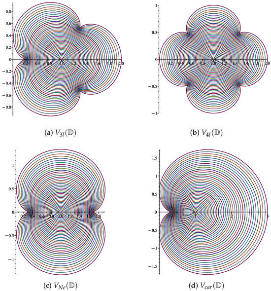
Figure 1. The domains $V_{3l}\left(\mathbb{D}\right)$, $V_{4l}\left(\mathbb{D}\right)$, $V_{Ne}\left(\mathbb{D}\right)$ and $V_{car}\left(\mathbb{D}\right)$.

Remark 2. (i) First, we will show that for appropriate choice of the parameters, the classes ${\mathcal{U}}_{a,b}^{l,q}$ and ${\mathcal{V}}_{a,b}^{l,q}$ are not empty, for a convenient function V. Thus, let us consider the function V to be given by $V\left(z\right):=V_{4l}\left(z\right)=1+{\displaystyle \frac{5}{6}}z+{\displaystyle \frac{1}{6}}{z}^5$. Like we proved in [23] ([Remark 1]), the function $V_{4l}$ is starlike (univalent) in $\mathbb{D}$ with respect to the point $w_0=1$; therefore, according to the equivalence (2), we should find values of the parameters such that

$${\Phi }_{a,b}^{l,q}\left[f\right]\left(\mathbb{D}\right)\subset V_{4l}\left(\mathbb{D}\right)\mathit{and}{\Psi }_{a,b}^{l,q}\left[f\right]\left(\mathbb{D}\right)\subset V_{4l}\left(\mathbb{D}\right),$$

where

$$\begin{array}{cc}\hfill {\Phi }_{a,b}^{l,q}\left[f\right]\left(z\right):=& (1-a){\displaystyle \frac{z^{1-b}{D}_{q}h\left(z\right)}{{\left(h\left(z\right)\right)}^{1-b}}}+a{\displaystyle \frac{z{\left(D_{q}h\left(z\right)\right)}^l}{h\left(z\right)}},\hfill \\ \hfill {\Psi }_{a,b}^{l,q}\left[f\right]\left(z\right):=& (1-a)\left(1+{\displaystyle \frac{z^{2-b}{D}_q\left(D_{q}h\left(z\right)\right)}{{\left(z{D}_{q}h\left(z\right)\right)}^{1-b}}}\right)+a{\displaystyle \frac{{\left({\left(z{D}_{q}h\left(z\right)\right)}^{\prime }\right)}^l}{D_{q}h\left(z\right)}}.\hfill \end{array}$$

Considering the function $\tilde{f}\left(z\right)=z+\alpha z^2+\beta z^3$, for the values $\alpha =0.6$, $\beta =0.1$, $a=0.9$, $b=0.7$, $q=0.2$ and $l=2$, using the 2D plot of the MAPLE™ 2025 computer software, we obtain the images of the boundary $\partial \mathbb{D}$ by the functions ${\Phi }_{a,b}^{l,q}\left[\tilde{f}\right]$ and $V_{4l}$ shown in Figure 2a. Since $V_{4l}$ is univalent in $\mathbb{D}$, the equivalence (2) yields that the subordination ${\Phi }_{a,b}^{l,q}\left[\tilde{f}\right]\left(z\right)\prec V_{4l}\left(z\right)$ holds whenever ${\Phi }_{a,b}^{l,q}\left[\tilde{f}\right]\left(0\right)=V_{4l}\left(0\right)=1$ and ${\Phi }_{a,b}^{l,q}\left[\tilde{f}\right]\left(\mathbb{D}\right)\subset V_{4l}\left(\mathbb{D}\right)$ (see Figure 2a). In conclusion, $\tilde{f}\in {\mathcal{U}}_{a,b}^{l,q}$ for the above values of the parameters; hence, the class ${\mathcal{U}}_{a,b}^{l,q}$ is not empty for non-trivial values of the parameters.

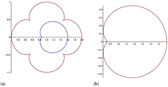
Figure 2. Figures for Remark 2 (i): (a) The images of ${\Phi }_{a,b}^{l,q}\left[\tilde{f}\right]\left({\mathrm{e}}^{\mathrm{i}\theta }\right)$ (blue color) and $V_{4l}\left({\mathrm{e}}^{\mathrm{i}\theta }\right)$ (red color), $\theta \in [0,2\pi )$. (b) The image of $\tilde{f}\left(\partial \mathbb{D}\right)$.

Let us recall the well known univalence theorem on the boundary (see, for example, [24] Lemma 1.1, p. 13): If f is analytic in $\overline{\mathbb{D}}$ and injective on the boundary $\partial \mathbb{D}$, then f is univalent in $\mathbb{D}$ and maps $\mathbb{D}$ onto the inner domain of the (closed) Jordan curve $J=f(\partial \mathbb{D})$.

For the above defined function $\tilde{f}$, we have $\tilde{f}\in {\mathcal{U}}_{a,b}^{l,q}$. Using the 2D plot of the MAPLE™ 2025 computer software, the image of the boundary $\partial \mathbb{D}$ by the functions $\tilde{f}$ (see Figure 2b), we see that $\tilde{f}\left(\partial \mathbb{D}\right)$ is a simple curve; hence, $\tilde{f}$ is univalent on $\partial \mathbb{D}$. Thus, from the above mentioned result, we conclude that $\tilde{f}\in \mathcal{S}$, consequently, ${\mathcal{U}}_{a,b}^{l,q}\cap \mathcal{S}\ne \varnothing$ for some values of the parameters $a\in [0,1]$, $b\ge 0$, $l\ge 1$ and $q\in (0,1)$.

(ii) Using similar reasons to the above, if we consider the function $\widehat{f}\left(z\right)=z+\alpha z^2+\beta z^3$, for the values $\alpha =0.7$, $\beta =0.1$, $a=0.9$, $b=0.7$, $q=0.1$ and $l=2$, using the 2D plot of the MAPLE™ 2025 computer software, we obtain the images of the boundary $\partial \mathbb{D}$ by the functions ${\Psi }_{a,b}^{l,q}\left[\tilde{f}\right]$ and $V_{4l}$, shown in Figure 3b. Thus, $\widehat{f}\in {\mathcal{V}}_{a,b}^{l,q}$ for the above values of the parameters and the class ${\mathcal{V}}_{a,b}^{l,q}$ is not empty for non-trivial values of the parameters.

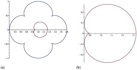
Figure 3. Figures for Remark 2 (ii): (a) The images of ${\Psi }_{a,b}^{l,q}\left[\widehat{f}\right]\left({\mathrm{e}}^{\mathrm{i}\theta }\right)$ (red color) and $V_{4l}\left({\mathrm{e}}^{\mathrm{i}\theta }\right)$ (blue color), $\theta \in [0,2\pi )$. (b) The image of $\widehat{f}\left(\partial \mathbb{D}\right)$.

Using the 2D plot of the MAPLE™ 2025 computer software, the image of the boundary $\partial \mathbb{D}$ by the functions $\widehat{f}$ (see Figure 3b), we obtain that $\widehat{f}\left(\partial \mathbb{D}\right)$ is a simple curve; hence, $\widehat{f}$ is univalent on $\partial \mathbb{D}$. We deduce that $\widehat{f}\in \mathcal{S}$, thus ${\mathcal{V}}_{a,b}^{l,q}\cap \mathcal{S}\ne \varnothing$ for some values of the parameters $a\in [0,1]$, $b\ge 0$, $l\ge 1$ and $q\in (0,1)$.

(iii) As shown in Figure 4a–d and using similar reasons as in the items (i) and (ii), we find that

$$f_{\ast }\left(z\right):=z+\alpha z^2+\beta z^3\in {\mathcal{U}}_{a,b}^{l,q}\setminus \mathcal{S}$$

for $\alpha =0.6$, $\beta =0.1$, $a=0.9$, $b=0.7$, $q=0.3$ and $l=2$, while

$$f_{\circ }\left(z\right):=z+\alpha z^2+\beta z^3\in {\mathcal{V}}_{a,b}^{l,q}\setminus \mathcal{S}$$

for $\alpha =0.8$, $\beta =0.2$, $a=0.8$, $b=0.7$, $q=0.1$ and $l=2$. Consequently, ${\mathcal{U}}_{a,b}^{l,q}\neg \subset \mathcal{S}$ and ${\mathcal{V}}_{a,b}^{l,q}\neg \subset \mathcal{S}$ for some values of the parameters.

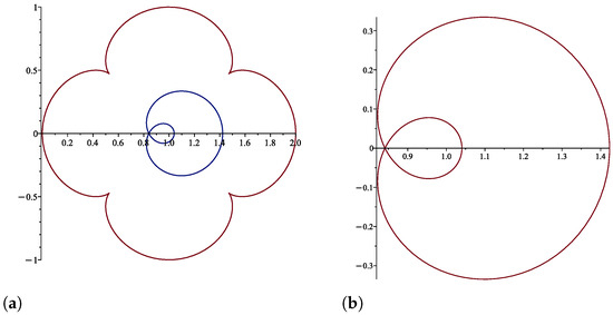
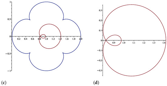
Figure 4. Figures for Remark 2 (iii): (a) The images of ${\Phi }_{a,b}^{l,q}\left[f_{\ast }\right]\left({\mathrm{e}}^{\mathrm{i}\theta }\right)$ (blue color) and $V_{4l}\left({\mathrm{e}}^{\mathrm{i}\theta }\right)$ (red color), $\theta \in [0,2\pi )$. (b) The image of $f_{\ast }\left(\partial \mathbb{D}\right)$. (c) The images of ${\Psi }_{a,b}^{l,q}\left[f_{\circ }\right]\left({\mathrm{e}}^{\mathrm{i}\theta }\right)$ (red color) and $V_{4l}\left({\mathrm{e}}^{\mathrm{i}\theta }\right)$ (blue color), $\theta \in [0,2\pi )$. (d) The image of $f_{\circ }\left(\partial \mathbb{D}\right)$.

Remark 3.

Within the realm of univalent function theory, which examines one-to-one (injective) analytic mappings, these particular epicycloidal and nephroid shapes are invaluable. They serve as precise target regions for the images of the unit disk under certain subclasses of univalent functions.

(i)

In [25], Gandhi introduced the class of starlike functions connected with three leaf functions by

$${\mathcal{S}}_{3l}^{\ast }:=\left\{h\in \mathcal{A}:{\displaystyle \frac{z{h}^{\prime }\left(z\right)}{h\left(z\right)}}\prec 1+{\displaystyle \frac{4}{5}}z+{\displaystyle \frac{1}{5}}{z}^4\right\}.$$

We mention that in 2022, the authors of the articles [26,27] introduced and studied various subclasses of analytic functions. These functions were defined through subordination to a four-leaf function, and their important properties were characterized.

(ii)

In 2020, Wani and Swaminathan [28] introduced the Ma–Minda subclass of starlike functions ${\mathcal{S}}_{Ne}^{\ast }$ by choosing $\varphi \left(z\right)=1+z-z^3/3$, associated with a nephroid-shaped domain, defined by

$${\mathcal{S}}_{Ne}^{\ast }=\left\{h\in \mathcal{A}:{\displaystyle \frac{z{h}^{\prime }\left(z\right)}{h\left(z\right)}}\prec 1+z-{\displaystyle \frac{z^3}{3}}\right\}.$$

Furthermore, in [29], Sharma et al. discussed the class ${\mathcal{S}}_{car}^{\ast }$, defined by

$${\mathcal{S}}_{car}^{\ast }:=\left\{h\in \mathcal{A}:{\displaystyle \frac{z{h}^{\prime }\left(z\right)}{h\left(z\right)}}\prec 1+{\displaystyle \frac{4}{3}}z+{\displaystyle \frac{2}{3}}{z}^2\right\}.$$

Remark 4.

We emphasize that for different choices of the parameters a, b and q, our classes defined by (9) and (10) reduce to the following ones:

(a)

Taking $a=0$ and $q\to 1^{-}$ in Definition 3, the class ${\mathcal{U}}_{a,b}^{l,q}$ reduces to ${\mathcal{U}}_{0,b}^{l,1^{-}}$, which is a subclass of the family of Bazilevič functions.

i.

Considering in addition $b=0$, these classes reduce to ${\mathcal{U}}_{0,0}^{l,1^{-}}$, which is known as the starlike functions class.

ii.

Moreover, for $b=1$, these classes reduce to ${\mathcal{U}}_{0,1}^{l,1^{-}}$, which is known as the bounded turning functions class.

(b)

Putting $a=1$ and $q\to 1^{-}$ in Definition 3, the class ${\mathcal{U}}_{a,b}^{l,q}$ reduces to ${\mathcal{U}}_{1,b}^{l,1^{-}}$, known as the family of 1-pseudo-starlike functions in the unit disk $\mathbb{D}$.

(c)

If we take $a=0$, $b=0$ and $q\to 1^{-}$ in Definition 2, the class ${\mathcal{V}}_{a,b}^{l,q}$ reduces to ${\mathcal{V}}_{0,0}^{l,1^{-}}$, which is the convex functions class.

(d)

Choosing $a=1$ and $q\to 1^{-}$ in Definition 2, the class ${\mathcal{V}}_{a,b}^{l,q}$ reduces to ${\mathcal{V}}_{1,b}^{l,1^{-}}$, known as the family of 1-pseudo-convex functions.

3. Preliminaries and Main Results

Let us define by $\mathcal{P}$ the well-known Carathéodory class, i.e., the family of holomorphic functions l in $\mathbb{D}$ that satisfies the condition $Rel\left(z\right)>0$$(z\in \mathbb{D})$ and having the form

$$l\left(z\right)=1+\sum _{n=1}^{\infty }{l}_n{z}^n,z\in \mathbb{D}.$$

(11)

We need the following lemmas in order to prove our results.

Lemma 1.

Let $l\in \mathcal{P}$ be of the form (11).

(i)

Then, for $n\ge 1$,

$$\left|l_n\right|\le 2.$$

(12)

The inequality holds for all $n\ge 1$ if and only if $l\left(z\right)={\displaystyle \frac{1+\lambda z}{1-\lambda z}}$, $\left|\lambda \right|=1$.

(ii)

Furthermore, if $\mu \ge 0$, then

$$\left|l_{n+k}-\mu l_n{l}_k\right|\le 2max\left\{1;|2\mu -1|\right\}=\left\{\begin{array}{cc}2,\hfill & \mathrm{if}0\le \mu \le 1,\hfill \\ 2|2\mu -1|,\hfill & \mathrm{otherwise}.\hfill \end{array}\right.$$

(13)

If $0<\mu <1$, the inequality is sharp for the function $l\left(z\right)={\displaystyle \frac{1+z^{n+k}}{1-z^{n+k}}}$. In the other cases, the inequality is sharp for the function $l\left(z\right)={\displaystyle \frac{1+z}{1-z}}$.

Note that the inequality (12) is the well-known result of the Carathéodory Lemma [30] (see also [24] ([ Corollary 2.3, p. 41]) and [3] ([Carathéodory Lemma, p. 41])). Inequality (13) represents Lemma 2.3 of [31], which for $\mu =1$ was proven in a more general form in [32] ([Lemma 1, p. 546]). We emphasize that the inequality (13) remains valid for all $\mu \in \mathbb{C}$ as it was proven in [33] ([Theorem 1]).

3.1. Initial Coefficients and Hankel Determinants for the Class ${\mathcal{U}}_{a,b}^{l,q}$

In this subsection, our main goal is to establish precise upper bounds for the initial coefficients, specifically $|a_2|$ and $|a_3|$. Additionally, we aim to investigate the Fekete–Szegő functional, given by $\left|a_3-\mu a_2^2\right|$, for functions within the specified class. We will also determine the modulus of the difference between the second Hankel determinant of a function and that of its inverse, i.e., $\left|H_{2,2}\left(h\right)-H_{2,2}\left(h^{-1}\right)\right|$.

Theorem 1.

Let the function $h\in \mathcal{A}$, given by (1), be a member of the class ${\mathcal{U}}_{a,b}^{l,q}$. Then,

$$\begin{array}{c}\hfill |a_2|\le {\displaystyle \frac{R_1}{\left|L\right|}},\hfill \end{array}$$

(14)

$$\begin{array}{cccccccccccc}& & & & & & & & & & & \hfill |a_3|\le {\displaystyle \frac{R_1}{\left|M\right|}}max\left\{1;\left|{\displaystyle \frac{R_2}{R_1}}-{\displaystyle \frac{U}{L^2}}{R}_1\right|\right\},\hfill \end{array}$$

(15)

where

$$\begin{array}{cc}\hfill L=& al{\left[2\right]}_q-ab-a{\left[2\right]}_q+b+{\left[2\right]}_q-1,\hfill \\ \hfill M=& al{\left[3\right]}_q-ab-{\left[3\right]}_{q}a+b+{\left[3\right]}_q-1,\hfill \\ \hfill U=& {\displaystyle \frac{3}{2}}ab-{\displaystyle \frac{1}{2}}a{b}^2-{\left[2\right]}_q+{\displaystyle \frac{1}{2}}{b}^2-{\displaystyle \frac{3}{2}}b+{\displaystyle \frac{1}{2}}a{l}^2{\left[2\right]}_q^2-ab{\left[2\right]}_q+a{\left[2\right]}_q+b{\left[2\right]}_q\hfill \\ \hfill & -{\displaystyle \frac{1}{2}}al{\left[2\right]}_q^2-al{\left[2\right]}_q+1.\hfill \end{array}$$

(16)

Proof. 

If $h\in {\mathcal{U}}_{a,b}^{l,q}$, from Definition 3 there exists an analytic function v with $v\left(0\right)=0$ and $\left|v\right(z\left)\right|<1$, $z\in \mathbb{D}$ such that

$$(1-a){\displaystyle \frac{z^{1-b}{D}_{q}h\left(z\right)}{{\left(h\left(z\right)\right)}^{1-b}}}+a{\displaystyle \frac{z{\left(D_{q}h\left(z\right)\right)}^l}{h\left(z\right)}}=V\left(v\left(z\right)\right),z\in \mathbb{D}.$$

(17)

Writing the Schwarz function v in terms of $p\in \mathcal{P}$, that is

$$p\left(z\right):={\displaystyle \frac{1+v\left(z\right)}{1-v\left(z\right)}}=1+p_{1}z+p_2{z}^2+p_3{z}^3+\dots ,z\in \mathbb{D},$$

which is equivalent to

$$\begin{array}{cc}\hfill v\left(z\right)={\displaystyle \frac{p\left(z\right)-1}{p\left(z\right)+1}}=& {\displaystyle \frac{1}{2}}{p}_{1}z+\left({\displaystyle \frac{1}{2}}{p}_2-{\displaystyle \frac{1}{4}}{p}_1^2\right)z^2+\left({\displaystyle \frac{1}{8}}{p}_1^3-{\displaystyle \frac{1}{2}}{p}_1{p}_2+{\displaystyle \frac{1}{2}}{p}_3\right)z^3\hfill \\ \hfill & +\left({\displaystyle \frac{1}{2}}{p}_4-{\displaystyle \frac{1}{2}}{p}_1{p}_3-{\displaystyle \frac{1}{4}}{p}_2^2-{\displaystyle \frac{1}{16}}{p}_1^4+{\displaystyle \frac{3}{8}}{p}_1^2{p}_2\right)z^4+\dots ,z\in \mathbb{D},\hfill \end{array}$$

(18)

we obtain

$$\begin{array}{cc}\hfill V\left(v\left(z\right)\right)& =1+R_{1}v\left(z\right)+R_2{\left(v\left(z\right)\right)}^2+R_3{\left(v\left(z\right)\right)}^3+\dots \hfill \\ \hfill & =1+{\displaystyle \frac{R_1{p}_{1}z}{2}}+\left({\displaystyle \frac{1}{2}}{R}_1{p}_2-{\displaystyle \frac{1}{4}}{R}_1{p}_1^2+{\displaystyle \frac{1}{4}}{R}_2{p}_1^2\right)z^2\hfill \\ \hfill & +\left({\displaystyle \frac{1}{2}}{R}_1{p}_3-{\displaystyle \frac{1}{2}}{R}_1{p}_1{p}_2+{\displaystyle \frac{1}{8}}{R}_1{p}_1^3-{\displaystyle \frac{1}{4}}{R}_2{p}_1^3+{\displaystyle \frac{1}{2}}{R}_2{p}_1{p}_2+{\displaystyle \frac{1}{8}}{R}_3{p}_1^3\right)z^3+\dots ,z\in \mathbb{D}.\hfill \end{array}$$

(19)

Since the function h has the form (1), it follows that

$$\begin{array}{cc}\hfill & (1-a){\displaystyle \frac{z^{1-b}{D}_{q}h\left(z\right)}{{\left(h\left(z\right)\right)}^{1-b}}}+a{\displaystyle \frac{z{\left(D_{q}h\left(z\right)\right)}^l}{h\left(z\right)}}=1+\left(al{\left[2\right]}_q-ab-a{\left[2\right]}_q+b+{\left[2\right]}_q-1\right)a_{2}z\hfill \\ \hfill & +[-{\displaystyle \frac{1}{2}}(-a{l}^2{\left[2\right]}_q^2+al{\left[2\right]}_q^2+a{b}^2+2ab{\left[2\right]}_q+2al{\left[2\right]}_q-3ab-2a{\left[2\right]}_q-b^2-2b{\left[2\right]}_q+3b\hfill \\ \hfill & +2{\left[2\right]}_q-2)a_2^2-a_3\left(-al{\left[3\right]}_q+ab+{\left[3\right]}_{q}a-b-{\left[3\right]}_q+1\right)]z^2\hfill \\ \hfill & +[\left(al{\left[4\right]}_q-ab-{\left[4\right]}_{q}a+b+{\left[4\right]}_q-1\right)a_4+(a{l}^2{\left[2\right]}_q{\left[3\right]}_q-al{\left[2\right]}_q{\left[3\right]}_q-a{b}^2-ab{\left[2\right]}_q-ab{\left[3\right]}_q\hfill \\ \hfill & -al{\left[2\right]}_q-al{\left[3\right]}_q+3ab+a{\left[2\right]}_q+{\left[3\right]}_{q}a+b^2+b{\left[2\right]}_q+b{\left[3\right]}_q-3b-{\left[2\right]}_q-{\left[3\right]}_q+2)a_2{a}_3\hfill \\ \hfill & +({\displaystyle \frac{11}{6}}b+{\displaystyle \frac{1}{6}}{b}^3+{\displaystyle \frac{1}{3}}al{\left[2\right]}_q^3-{\displaystyle \frac{1}{2}}a{l}^2{\left[2\right]}_q^3+{\displaystyle \frac{1}{6}}a{l}^3{\left[2\right]}_q^3-{\displaystyle \frac{1}{2}}a{l}^2{\left[2\right]}_q^2+{\displaystyle \frac{1}{2}}al{\left[2\right]}_q^2+al{\left[2\right]}_q-{\displaystyle \frac{1}{2}}a{b}^2{\left[2\right]}_q\hfill \\ \hfill & +{\displaystyle \frac{3}{2}}ab{\left[2\right]}_q-a{\left[2\right]}_q-{\displaystyle \frac{11}{6}}ab-{\displaystyle \frac{1}{6}}{b}^{3}a+a{b}^2+{\displaystyle \frac{1}{2}}{b}^2{\left[2\right]}_q-{\displaystyle \frac{3}{2}}b{\left[2\right]}_q-1-b^2+{\left[2\right]}_q\left)a_2^3\right]z^3+\dots ,\hfill \end{array}$$

(20)

and equating the coefficients of “z” and “$z^2$” from the relations (19) and (20), we obtain

$$\begin{array}{cccccc}& & & & \hfill a_2=& {\displaystyle \frac{R_1{p}_1}{2\left(al{\left[2\right]}_q-ab-a{\left[2\right]}_q+b+{\left[2\right]}_q-1\right)}}={\displaystyle \frac{R_1{p}_1}{2L}},\hfill \end{array}$$

(21)

$$\begin{array}{cc}\hfill a_3=& {\displaystyle \frac{R_1}{2M}}\left[p_2-p_1^2\left({\displaystyle \frac{1}{2}}+{\displaystyle \frac{R_2}{2R_1}}-{\displaystyle \frac{U}{2L^2}}{R}_1\right)\right],\hfill \end{array}$$

(22)

where L, M and U are given by (16).

Taking the modules on the both sides of (21) and using the inequality (12) of Lemma 1, we obtain our desired result (14). Similarly, from the modules on both sides of (22), applying the inequality (13) of Lemma 1, we obtain the estimation (15). □

Remark 5. (i) The values of $|a_2|$ and the upper bounds for $|a_2|$ for the particular functions V considered in the Table 1 will be those shown in Table 2.

Table 2. Upper bounds for $|a_2|$ in the cases $V_{3l}$, $V_{4l}$, $V_{Ne}$ and $V_{car}$.

Function	The Upper Bound of $|{\mathit{a}}_2|$	The Limit of the Upper Bound if $\mathit{q}\to {\mathbf{1}}^{-}$
$V_{3l}\left(z\right)=1+{\displaystyle \frac{4}{5}}z+{\displaystyle \frac{1}{5}}{z}^4$	${\displaystyle \frac{4}{5\left|al{\left[2\right]}_q-ab-a{\left[2\right]}_q+b+{\left[2\right]}_q-1\right|}}$	${\displaystyle \frac{4}{5\left|2al-ab-2a+b+1\right|}}$
$V_{4l}\left(z\right)=1+{\displaystyle \frac{5}{6}}z+{\displaystyle \frac{1}{6}}{z}^5$	${\displaystyle \frac{5}{6\left|al{\left[2\right]}_q-ab-a{\left[2\right]}_q+b+{\left[2\right]}_q-1\right|}}$	${\displaystyle \frac{5}{6\left|2al-ab-2a+b+1\right|}}$
$V_{Ne}\left(z\right)=1+z-{\displaystyle \frac{z^3}{3}}$	${\displaystyle \frac{1}{\left|al{\left[2\right]}_q-ab-a{\left[2\right]}_q+b+{\left[2\right]}_q-1\right|}}$	${\displaystyle \frac{1}{\left|2al-ab-2a+b+1\right|}}$
$V_{car}\left(z\right)=1+{\displaystyle \frac{4}{3}}z+{\displaystyle \frac{2}{3}}{z}^2$	${\displaystyle \frac{4}{3\left|al{\left[2\right]}_q-ab-a{\left[2\right]}_q+b+{\left[2\right]}_q-1\right|}}$	${\displaystyle \frac{4}{3\left|2al-ab-2a+b+1\right|}}$

(ii) For the same functions V, if $q\to 1^{-}$, the upper bounds for $|a_3|$ are the next ones:

a.

For $V_{3l}\left(z\right)=1+{\displaystyle \frac{4}{5}}z+{\displaystyle \frac{1}{5}}{z}^4$ we obtain

$$\begin{array}{c}|a_3|\le {\displaystyle \frac{4}{5\left|3al-ab-3a+b+2\right|}}·\hfill \\ \hfill max\left\{1;{\displaystyle \frac{4}{5}}\left|{\displaystyle \frac{\frac{3}{2}ab-\frac{1}{2}a{b}^2+\frac{1}{2}{b}^2-\frac{3}{2}b+2\left(a{l}^2-ab+a+b-2al\right)-1}{{\left(2al-ab-2a+b+1\right)}^2}}\right|\right\}.\end{array}$$

b.

If $V_{4l}\left(z\right)=1+{\displaystyle \frac{5}{6}}z+{\displaystyle \frac{1}{6}}{z}^5$, then

$$\begin{array}{c}|a_3|\le {\displaystyle \frac{5}{6|3al-ab-3a+b+2|}}·\hfill \\ \hfill max\left\{1;{\displaystyle \frac{5}{6}}\left|{\displaystyle \frac{\frac{3}{2}ab-\frac{1}{2}a{b}^2+\frac{1}{2}{b}^2-\frac{3}{2}b+2\left(a{l}^2-ab+a+b-2al\right)-1}{{\left(2al-ab-2a+b+1\right)}^2}}\right|\right\}.\end{array}$$

c.

In the case $V_{Ne}\left(z\right)=1+z-{\displaystyle \frac{z^3}{3}}$, we have

$$\begin{array}{c}|a_3|\le {\displaystyle \frac{1}{|3al-ab-3a+b+2|}}·\hfill \\ \hfill max\left\{1;\left|{\displaystyle \frac{\frac{3}{2}ab-\frac{1}{2}a{b}^2+\frac{1}{2}{b}^2-\frac{3}{2}b+2\left(a{l}^2-ab+a+b-2al\right)-1}{{\left(2al-ab-2a+b+1\right)}^2}}\right|\right\}.\end{array}$$

d.

For $V_{car}\left(z\right)=1+{\displaystyle \frac{4}{3}}z+{\displaystyle \frac{2}{3}}{z}^2$, we obtain

$$\begin{array}{c}|a_3|\le {\displaystyle \frac{4}{3|3al-ab-3a+b+2|}}·\hfill \\ \hfill max\left\{1;{\displaystyle \frac{4}{3}}\left|{\displaystyle \frac{\frac{3}{2}ab-\frac{1}{2}a{b}^2+\frac{1}{2}{b}^2-\frac{3}{2}b+2\left(a{l}^2-ab+a+b-2al\right)-1}{{\left(2al-ab-2a+b+1\right)}^2}}\right|\right\}.\end{array}$$

The next theorem gives the bound of Fekete–Szegő functional for the class ${\mathcal{U}}_{a,b}^{l,q}$.

Theorem 2.

If $h\in {\mathcal{U}}_{a,b}^{l,q}$ has the form (1), then for any complex number μ, we have

$$\left|a_3-\mu a_2^2\right|\le {\displaystyle \frac{R_1}{\left|M\right|}}max\left\{1;\left|{\displaystyle \frac{R_2}{R_1}}-{\displaystyle \frac{U}{L^2}}{R}_1+\mu {\displaystyle \frac{M{R}_1}{L^2}}\right|\right\},$$

(23)

with L, M and U given by (16).

Proof. 

If $h\in {\mathcal{U}}_{a,b}^{l,q}$, using the relations (21) and (22), we obtain

$$\begin{array}{cc}\hfill a_3-\mu a_2^2& ={\displaystyle \frac{R_1}{2M}}\left[p_2-p_1^2\left\{{\displaystyle \frac{1}{2}}+{\displaystyle \frac{R_2}{2R_1}}-{\displaystyle \frac{U}{2L^2}}{R}_1+\mu {\displaystyle \frac{M{R}_1}{2L^2}}\right\}\right].\hfill \end{array}$$

(24)

Taking the modules on both sides of (24) and then applying the inequality (13) of Lemma 1, which remains valid—as we already mentioned—for all $\mu \in \mathbb{C}$, it follows

$$\left|a_3-\mu a_2^2\right|={\displaystyle \frac{R_1}{2\left|M\right|}}|p_2-p_1^2\left\{{\displaystyle \frac{1}{2}}+{\displaystyle \frac{R_2}{2R_1}}-{\displaystyle \frac{U}{2L^2}}{R}_1+\mu {\displaystyle \frac{M{R}_1}{2L^2}}\right\}|\le {\displaystyle \frac{R_1}{\left|M\right|}}max\left\{1;|2\mu -1|\right\},$$

where

$$\mu ={\displaystyle \frac{1}{2}}+{\displaystyle \frac{R_2}{2R_1}}-{\displaystyle \frac{U}{2L^2}}{R}_1+\mu {\displaystyle \frac{M{R}_1}{2L^2}},$$

which represents conclusion (23) of our result. □

For the Hankel determinants $H_{2,2}$ of the functions h and $h^{-1}$ given by (3), the following result holds:

Theorem 3.

If $h\in {\mathcal{U}}_{a,b}^{l,q}$ has the form (1), then we have

$$\left|H_{2,2}\left(h\right)-H_{2,2}\left(h^{-1}\right)\right|\le {\displaystyle \frac{R_1^3}{{\left|M\right|\left|L\right|}^2}}max\left\{1;\left|{\displaystyle \frac{M{R}_1}{L^2}}+{\displaystyle \frac{R_2}{R_1}}-{\displaystyle \frac{U{R}_1}{L^2}}\right|\right\},$$

(25)

where L, M and U are defined by (16).

Proof. 

Combining the relations (21) and (22) in the equality (6), we obtain

$$\begin{array}{cc}\hfill H_{2,2}\left(h\right)-H_{2,2}\left(h^{-1}\right)& =a_2^2\left(-a_2^2+a_3\right)\hfill \\ \hfill & =-{\displaystyle \frac{R_1^4{p}_1^4}{16L^4}}+{\displaystyle \frac{R_1^3{p}_1^2{p}_2}{8M{L}^2}}-{\displaystyle \frac{p_1^4{R}_1^3}{16L^{2}M}}-{\displaystyle \frac{p_1^4{R}_1^2{R}_2}{16L^{2}M}}+{\displaystyle \frac{p_1^4{R}_1^{4}U}{16L^{4}M}}\hfill \\ \hfill & ={\displaystyle \frac{R_1^3{p}_1^2}{8M{L}^2}}\left[p_2-p_1^2\left({\displaystyle \frac{M{R}_1}{2L^2}}+{\displaystyle \frac{1}{2}}+{\displaystyle \frac{R_2}{2R_1}}-{\displaystyle \frac{U{R}_1}{2L^2}}\right)\right].\hfill \end{array}$$

(26)

Taking the modules on both sides of (26), from the inequality (13) of Lemma 1, we obtain our conclusion (25). □

Remark 6.

Taking $q\to 1^{-}$, $a=b=0$ or $a=0$, $b=1$ in (25) we could obtain simple forms of the majorant for $\left|H_{2,2}\left(h\right)-H_{2,2}\left(h^{-1}\right)\right|$ if $h\in {\mathcal{U}}_{a,b}^{l,q}$ and V is replaced by $V_{3l}$, $V_{4l}$, $V_{Ne}$ and $V_{car}$.

3.2. Initial Coefficients and Hankel Determinants for the Class ${\mathcal{V}}_{a,b}^{l,q}$

In this subsection, our aim is to establish upper bounds for the coefficients $|a_2|$ and $|a_3|$ and for the Fekete–Szegő functional $\left|a_3-\mu a_2^2\right|$ if $h\in {\mathcal{V}}_{a,b}^{l,q}$. Moreover, we will analyze the existence of a majorant for difference between the second Hankel determinants of a function and its inverse, that is, $\left|H_{2,2}\left(h\right)-H_{2,2}\left(h^{-1}\right)\right|$.

Theorem 4.

Let the function $h\in \mathcal{A}$ given by (1) be a member of the class ${\mathcal{V}}_{a,b}^{l,q}$. Then,

$$\begin{array}{cc}\hfill |a_2|& \le {\displaystyle \frac{R_1}{\left|A\right|}},\hfill \end{array}$$

(27)

$$\begin{array}{ccccccccccccccc}& & & & & & & & & & & & & \hfill |a_3|& \le {\displaystyle \frac{R_1}{\left|B\right|}}max\left\{1;|-{\displaystyle \frac{R_2}{R_1}}+{\displaystyle \frac{G{R}_1}{A^2}}|\right\},\hfill \end{array}$$

(28)

where

$$\begin{array}{cc}\hfill \hfill & A=2al{\left[2\right]}_q-2a{\left[2\right]}_q+{\left[2\right]}_q,\hfill \\ \hfill \hfill & B=al{\left[2\right]}_q{\left[3\right]}_q+al{\left[3\right]}_q-a{\left[2\right]}_q{\left[3\right]}_q-a{\left[3\right]}_q+{\left[2\right]}_q{\left[3\right]}_q,\hfill \\ \hfill \hfill & G=2a{l}^2{\left[2\right]}_q^2-ab{\left[2\right]}_q^2-4al{\left[2\right]}_q^2+2a{\left[2\right]}_q^2+b{\left[2\right]}_q^2-{\left[2\right]}_q^2.\hfill \end{array}$$

(29)

Proof. 

If $h\in {\mathcal{V}}_{a,b}^{l,q}$, by Definition 4 there exists an analytic function v with $v\left(0\right)=0$ and $\left|v\right(z\left)\right|<1$, $z\in \mathbb{D}$ such that

$$(1-a)\left(1+{\displaystyle \frac{z^{2-b}{D}_q\left(D_{q}h\left(z\right)\right)}{{\left(z{D}_{q}h\left(z\right)\right)}^{1-b}}}\right)+a{\displaystyle \frac{{\left({\left(z{D}_{q}h\left(z\right)\right)}^{\prime }\right)}^l}{D_{q}h\left(z\right)}}=V\left(v\left(z\right)\right).$$

(30)

Since the function h has the form (1), it follows that

$$\begin{array}{cc}\hfill (1-a)\left(1+{\displaystyle \frac{z^{2-b}{D}_q\left(D_{q}h\left(z\right)\right)}{{\left(z{D}_{q}h\left(z\right)\right)}^{1-b}}}\right)& +a{\displaystyle \frac{{\left({\left(z{D}_{q}h\left(z\right)\right)}^{\prime }\right)}^l}{D_{q}h\left(z\right)}}=1+\left[\left(2al-2a+1\right){\left[2\right]}_q\right]a_{2}z\hfill \\ \hfill & +[{\left[3\right]}_q\left(al{\left[2\right]}_q+al-a{\left[2\right]}_q-a+{\left[2\right]}_q\right)a_3\hfill \\ \hfill & +\left(2a{l}^2-ab-4al+2a+b-1\right){\left[2\right]}_q^2{a}_2^2]z^2+\dots ,z\in \mathbb{D},\hfill \end{array}$$

(31)

and equating the coefficients of “z” and “$z^2$” from the relations (19) and (31), using the notations (29), we obtain

$$\begin{array}{ccc}& \hfill a_2& ={\displaystyle \frac{R_1{p}_1}{2\left(2al{\left[2\right]}_q-2a{\left[2\right]}_q+{\left[2\right]}_q\right)}}={\displaystyle \frac{R_1{p}_1}{2A}},\hfill \end{array}$$

(32)

$$\begin{array}{cc}\hfill a_3& ={\displaystyle \frac{R_1}{2B}}\left[p_2-p_1^2\left({\displaystyle \frac{1}{2}}-{\displaystyle \frac{R_2}{2R_1}}+{\displaystyle \frac{G{R}_1}{2A^2}}\right)\right].\hfill \end{array}$$

(33)

Taking modulus on both sides of (32) and applying the inequality (12) of Lemma 1, we obtain the first result (27). Finally, from the module of (33) combined with the inequality (13) of Lemma 1, we find the desired estimation (29). □

Remark 7.

Similarly to Remark 6, taking $q\to 1^{-}$, $a=b=0$ or $a=0$, $b=1$ in (27), (28) and replacing V by $V_{3l}$, $V_{4l}$, $V_{Ne}$ and $V_{car}$, we could find simple forms of the majorant for $\left|a_2\right|$ and $\left|a_3\right|$ if $h\in {\mathcal{V}}_{a,b}^{l,q}$.

The next theorem gives the bound of the Fekete–Szegő functional for the class ${\mathcal{V}}_{a,b}^{l,q}$.

Theorem 5.

If $h\in {\mathcal{V}}_{a,b}^{l,q}$ has the form (1), then for any complex number μ, we have

$$\left|a_3-\mu a_2^2\right|\le {\displaystyle \frac{R_1}{\left|B\right|}}max\left\{1;\left|-{\displaystyle \frac{R_2}{R_1}}+{\displaystyle \frac{G{R}_1}{A^2}}+\mu {\displaystyle \frac{R_{1}B}{A^2}}\right|\right\},$$

where A, B and G are defined by (29).

Proof. 

If $h\in {\mathcal{V}}_{a,b}^{l,q}$, using the equalities of (32) and (33), we obtain

$$\begin{array}{cc}\hfill a_3-\mu a_2^2& ={\displaystyle \frac{R_1}{2B}}\left[p_2-p_1^2\left({\displaystyle \frac{1}{2}}-{\displaystyle \frac{R_2}{2R_1}}+{\displaystyle \frac{G{R}_1}{2A^2}}+\mu {\displaystyle \frac{R_{1}B}{2A^2}}\right)\right].\hfill \end{array}$$

(34)

Taking now the modules on both sides of (34) and then applying the inequality (13) of Lemma 1, our result follows immediately. □

For the difference $\left|H_{2,2}\left(h\right)-H_{2,2}\left(h^{-1}\right)\right|$ of the $H_{2,2}$ Hankel determinants of $h\in {\mathcal{V}}_{a,b}^{l,q}$ and $h^{-1}$, we obtain the next estimation:

Theorem 6.

If $h\in {\mathcal{V}}_{a,b}^{l,q}$ has the form (1), then we have

$$\left|H_{2,2}\left(h\right)-H_{2,2}\left(h^{-1}\right)\right|\le {\displaystyle \frac{R_1^3}{A^2\left|B\right|}}max\left\{1;\left|-{\displaystyle \frac{R_2}{R_1}}+{\displaystyle \frac{G{R}_1}{A^2}}+{\displaystyle \frac{R_{1}B}{A^2}}\right|\right\},$$

where A, B and G are defined by (29).

Proof. 

Replacing the relations (32) and (33) in (6), one may obtain

$$\begin{array}{cc}\hfill H_{2,2}\left(h\right)-H_{2,2}\left(h^{-1}\right)& =a_2^2\left(-a_2^2+a_3\right)\hfill \\ \hfill & ={\displaystyle \frac{R_1^2{p}_1^2}{4A^2}}\left[{\displaystyle \frac{R_1{p}_2}{2B}}+\left(-{\displaystyle \frac{R_1}{4B}}+{\displaystyle \frac{R_2}{4B}}-{\displaystyle \frac{G{R}_1^2}{4A^{2}B}}-{\displaystyle \frac{R_1^2}{4A^2}}\right)p_1^2\right]\hfill \\ \hfill & ={\displaystyle \frac{R_1^3{p}_1^2}{8A^{2}B}}\left[p_2-\left({\displaystyle \frac{1}{2}}-{\displaystyle \frac{R_2}{2R_1}}+{\displaystyle \frac{G{R}_1}{2A^2}}+{\displaystyle \frac{R_{1}B}{2A^2}}\right)p_1^2\right],\hfill \end{array}$$

(35)

and taking the modules on both sides of (35) and applying (13) of Lemma 1 in the resulting relation, we obtain the required inequality. □

4. Concluding Remarks

In this paper, we introduced and characterized a new class of analytic functions in the open unit disk that consists of univalent and non-univalent functions, like we mentioned in the paper. We explored fundamental bounding properties of this class like the initial coefficients bounds, which provide insights into the local behavior of the functions.

A key achievement was establishing majorants for the Fekete–Szegő functional, offering bounds for the second coefficient and highlighting the geometric features of these functions. We also computed the modules of the difference from the second Hankel determinant and the second Hankel determinant for the inverse coefficients.

We believe that the importance of the actual results reside in the following:

–

the new definitions that extend some previous subclasses obtained for the special choices of the function V from the right-hand sides of the subordinations (9) and (10);

–

the connections between the q-calculus given by the q-analogues of the derivatives and the Geometric Function Theory of one variable function;

–

the possibility to determine upper bounds of the first coefficients for these classes;

–

the fact that it was possible to obtain results related to the Fekete–Szegő functionals;

–

the estimations for the differences of particular Hankel determinants of the functions and their inverses for these classes.

That are specific problems in this field of interest. These findings enrich the literature on analytic functions and provide a framework for future research. The established bounds and geometric properties pave the way for exploring subclasses, convolution properties and applications in related fields. Future work could focus on higher-order Hankel determinants and connections with other function classes.

References

- Lindelöf, E. Mémoire sur certaines inégalités dans la théorie des fonctions monogènes et quelques propriétés nouvelles de ces fonctions dans le voisinage d’un point singulier essentiel. Acta Soc. Sci. Fenn. 1909, 35, 1–35. [Google Scholar]
- De Branges, L. A proof of the Bieberbach conjecture. Acta Math. 1985, 154, 137–152. [Google Scholar] [CrossRef]
- Duren, P.L. Univalent Functions. Grundlehren der Mathematischen Wissenschaften, Band 259; Springer: New York, NY, USA; Berlin/Heidelberg, Germany; Tokyo, Japan, 2001. [Google Scholar]
- Noonan, W.; Thomas, D.K. On the second Hankel determinant of areally mean p-valent functions. Trans. Am. Math. Soc. 1976, 223, 337–346. [Google Scholar] [CrossRef]
- Fekete, M.; Szegő, G. Eine Bemerkung Über Ungerade Schlichte Funktionen. J. Lond. Math. Soc. 1933, 1–8, 81–160. [Google Scholar] [CrossRef]
- Srivastava, H.M.; Khan, N.; Darus, M.; Khan, S.; Ahamad, Q.Z.; Hussain, S. Fekete-Szegő type problems and their applications for a subclass of q-starlike functions with respect to symmetrical points. Mathematics 2020, 8, 842. [Google Scholar] [CrossRef]
- Srivastava, H.M.; Shaba, T.G.; Murugusundaramoorthy, G.; Wanas, A.K.; Oros, G.I. The Fekete-Szegő functional and the Hankel determinant for a certain class of analytic functions involving the Hohlov operator. AIMS Math. 2022, 8, 340–360. [Google Scholar] [CrossRef]
- Alsoboh, A.; Çağlar, M.; Buyankara, M. Fekete-Szegő inequality for a subclass of bi-univalent functions linked to q-ultraspherical polynomials. Contemp. Math. 2024, 5, 2531–2545. [Google Scholar] [CrossRef]
- Marimuthu, K.; Uma, J.; Bulboacă, T. Coefficient estimates for starlike and convex functions associated with cosine function. Hacet. J. Math. Stat. 2023, 52, 596–618. [Google Scholar]
- Murugusundaramoorthy, G.; Magesh, N. Coefficient inequalities for certain classes of analytic functions associated with Hankel determinant. Bull. Math. Anal. Appl. 2009, 1, 85–89. [Google Scholar]
- Panigrahi, T.; Murugusundarmoorthy, G. Second Hankel determinant for a subclass of analytic function defined by Sălăgean-difference operator. Mat. Stud. 2022, 57, 147–156. [Google Scholar] [CrossRef]
- Singh, R. On Bazilevič functions. Proc. Am. Math. Soc. 1973, 38, 261–271. [Google Scholar] [CrossRef]
- Babalola, K.O. On λ-pseudo-starlike functions. J. Class. Anal. 2013, 3, 137–147. [Google Scholar] [CrossRef]
- Janani, T.; Murugusundaramoorthy, G. Zalcman functional for class of λ-pseudo starlike functions associated with sigmoid function. Bull. Transilv. Univ. Braşov. Ser. III Math. Comput. Sci. 2018, 11, 77–84. [Google Scholar]
- Murugusundaramoorthy, G.; Janani, T. Sigmoid function in the space of univalent λ-pseudo starlike functions. Inter. J. Pure Appl. Math. 2015, 101, 33–41. [Google Scholar] [CrossRef]
- Sokół, J.; Murugusundaramoorthy, G.; Vijaya, K. On λ-pseudo starlike functions associated with vertical strip domain. Asian-Eur. J. Math. 2023, 16, 2350135. [Google Scholar] [CrossRef]
- Jackson, F.H. On q-functions and a certain difference operator. Earth Environ. Sci. Tran. R. Soc. Edinb. 1909, 46, 253–281. [Google Scholar] [CrossRef]
- Jackson, F.H. On q-definite integrals. Quart. J. Pure Appl. Math. 1910, 41, 193–203. [Google Scholar]
- Aral, A.; Gupta, V. On q-Baskakov type operators. Demonstr. Math. 2009, 42, 109–122. [Google Scholar] [PubMed]
- Aral, A.; Gupta, V. Generalized q-Baskakov operators. Math. Slovaca 2011, 61, 619–634. [Google Scholar] [CrossRef]
- Anastassiou, G.A.; Gal, S.G. Geometric and approximation properties of generalized singular integrals in the unit disk. J. Korean Math. Soc. 2006, 23, 425–443. [Google Scholar] [CrossRef]
- Kanas, S.; Răducanu, D. Some class of analytic functions related to conic domains. Math. Slovaca 2014, 64, 1183–1196. [Google Scholar] [CrossRef]
- Gunasekar, S.; Sudharsanan, B.; Ibrahim, M.; Bulboacă, T. Subclasses of analytic functions subordinated to the four-leaf function. Axioms 2024, 13, 155. [Google Scholar] [CrossRef]
- Pommerenke, C. Univalent Functions; Vandenhoeck and Ruprecht: Göttingen, Germany, 1975. [Google Scholar]
- Gandhi, S. Radius estimates for three leaf function and convex combination of starlike functions. In Proceedings of the International Conference on Recent Advances in Pure and Applied Mathematics, New Delhi, India, 23–25 December 2018; Springer: Singapore, 2018; pp. 173–184. [Google Scholar]
- Alshehry, A.S.; Shah, R.; Bariq, A. The second Hankel determinant of logarithmic coefficients for starlike and convex functions involving four-leaf-shaped domain. J. Funct. Spaces 2022, 2022, 2621811. [Google Scholar] [CrossRef]
- Sunthrayuth, P.; Jawarneh, Y.; Naeem, M.; Iqbal, N.; Kafle, J. Some sharp results on coefficient estimate problems for four-leaf-type bounded turning functions. J. Funct. Spaces 2022, 2022, 8356125. [Google Scholar] [CrossRef]
- Wani, L.A.; Swaminathan, A. Radius problems for functions associated with a nephroid domain. Rev. Real Acad. Cienc. Exactas Fís. Nat. Ser. A Matemáticas RACSAM 2020, 114, 178. [Google Scholar] [CrossRef]
- Sharma, K.; Jain, N.K.; Ravichandran, V. Starlike functions associated with a cardioid. Afr. Mat. 2016, 27, 923–939. [Google Scholar] [CrossRef]
- Carathéodory, C. Über den Variabilitätsbereich der Koeffizienten von Potenzreihen, die gegebene Werte nicht annehmen. Math. Ann. 1907, 64, 95–115. [Google Scholar] [CrossRef]
- Ravichandran, V.; Verma, S. Bound for the fifth coefficient of certain starlike functions. C. R. Acad. Sci. Paris Ser. 1 2015, 353, 505–510. [Google Scholar] [CrossRef]
- Livingston, A.E. The coefficients of multivalent close-to-convex functions. Proc. Am. Math. Soc. 1969, 21, 545–552. [Google Scholar] [CrossRef]
- Efraimidis, I. A generalization of Livingston’s coefficient inequalities for functions with positive real part. J. Math. Anal. Appl. 2016, 435, 369–379. [Google Scholar] [CrossRef]
Disclaimer/Publisher’s Note: The statements, opinions and data contained in all publications are solely those of the individual author(s) and contributor(s) and not of MDPI and/or the editor(s). MDPI and/or the editor(s) disclaim responsibility for any injury to people or property resulting from any ideas, methods, instructions or products referred to in the content. |
© 2026 by the authors. Licensee MDPI, Basel, Switzerland. This article is an open access article distributed under the terms and conditions of the Creative Commons Attribution (CC BY) license.