Nonlocal Extensions of First Order Initial Value Problems

Abstract

We study certain Volterra integral equations that extend and recover first order ordinary differential equations (ODEs). We formulate the former equations from the latter by replacing classical derivatives with nonlocal integral operators with anti-symmetric kernels. Replacements of spatial derivatives have seen success in fracture mechanics, diffusion, and image processing. In this paper, we consider nonlocal replacements of time derivatives which contain future data. To account for the nonlocal nature of the operators, we formulate initial “volume” problems (IVPs) for these integral equations; the initial data is prescribed on a time interval rather than at a single point. As a nonlocality parameter vanishes, we show that the solutions to these equations recover those of classical ODEs. We demonstrate this convergence with exact solutions of some simple IVPs. However, we find that the solutions of these nonlocal models exhibit several properties distinct from their classical counterparts. For example, the solutions exhibit discontinuities at periodic intervals. In addition, for some IVPs, a continuous initial profile develops a measure-valued singularity in finite time. At subsequent periodic intervals, these solutions develop increasingly higher order distributional singularities.

1. Introduction

Many physical problems are formulated in terms of differential equations. A common example is the following ordinary differential equation (ODE) for function $u:\mathbb{R}\to \mathbb{R}$:

$$\begin{array}{c}\hfill u^{\prime }\left(t\right)=F(t,u\left(t\right)),t\in \mathbb{R}.\end{array}$$

(1)

Although solutions of (1) describe a wide range of physical behaviors, they cannot do so when the physical phenomenon at hand is singular. For example, the derivative $u^{\prime }$ is undefined where u has a discontinuity, and Equation (1) no longer makes sense. Even if only the “forcing term” F has a discontinuity, the analysis [1] and numerical solving [2] of (1) are not straightforward, since u is still not differentiable.

A solution to this difficulty implemented for partial differential equations (PDEs) is to replace the classical derivative $d/dt$ in (1) with an integral operator, which we call a “nonlocal derivative”. Following [3], we define the nonlocal derivative as follows:

$$\begin{array}{c}\hfill D_{\alpha ,ϵ}u\left(t\right):=-{\alpha }_{ϵ}\ast u\left(t\right)={\int }_{-\infty }^{\infty }{\alpha }_{ϵ}(s-t)u\left(s\right)\mathrm{d}s,t\in \mathbb{R},\end{array}$$

(2)

where $ϵ>0$ is a “nonlocality parameter”, and ${\alpha }_{ϵ}$ is an anti-symmetric integral kernel. As $ϵ\to 0$, we require $D_{\alpha ,ϵ}\to d/dt$ in some sense. This makes $D_{\alpha ,ϵ}$ a “nonlocal extension” of the classical derivative. We call the following integral equation for $u_{ϵ}:\mathbb{R}\to \mathbb{R}$

$$\begin{array}{c}\hfill D_{\alpha ,ϵ}{u}_{ϵ}\left(t\right)=F(t,u_{ϵ}\left(t\right)),t\in \mathbb{R},\end{array}$$

(3)

a nonlocal extension of the ODE (1). As $ϵ\to 0$, we expect to recover the classical solution via $u_{ϵ}\to u$.

Nonlocal extensions of classical models have garnered broad success in describing nonclassical physical phenomena. Nonlocal operators, such as fractional derivatives, have been known since the 1800s, but such nonlocal extensions have recently found successful application in Silling’s [4] theory of peridynamic fractures. There are more applications of these nonlocal operators to anomalous diffusion [5,6] and image processing [7].

The success of nonlocal operators stems from the ease with which they handle singularities. Although classical models using differential equations such as (1) cannot well describe discontinuous phenomena, such as those occurring in fracture dynamics, the integral operators applied by Silling suffer no such difficulties. As opposed to the differentiability required by $d/dt$, the integral operator $D_{\alpha ,ϵ}$ only requires some form of integrability. Using nonlocal operators in these classical models extends the types of physical processes that we can model and the types of qualitative behavior that we can describe.

The extensivity property is also an important feature of these nonlocal models. In [3], it is shown that such first order nonlocal operators converge strongly in $L^2$ to classical partial derivatives as $ϵ\to 0$. Classical models are often physically correct descriptions. We want to retain these successful classical results when considering more general models. In addition to describing more phenomena, nonlocal extensions can correctly describe classical behavior by passing to to the classical limit of $ϵ\to 0$.

The majority of the nonlocal literature has focused on so-called second order models. These nonlocal models extend second order partial differential equations and boundary value problems, such as the wave equation [8], Laplace’s equation [9], and the heat equation [6] (see also the nonlocal counterpart to the fourth order biharmonic equation [10]).

Given the success of these nonlocal operators in extending second order models, we are interested in their application to first order ODEs. These equations are very important in practical arenas, but nonlocal extensions do not appear to have been explored. Du et al. [11] studied a nonlocal extension of the nonlinear advection equation, a first order PDE. One interesting result of theirs stipulates that nonlocal advection solutions do not blow up in finite time, a stark contrast to classical solutions. There is also some literature available for first order models using fractional derivatives (see [12] for a large set of examples).

As a first step, we propose a nonlocal extension for the classical initial value problem. We call this extension an initial volume problem (IVP). Using exact solutions of some simple IVPs, we demonstrate both the convergence of the solutions to their classical counterparts as well as some interesting features that nonlocality brings to the table. We also show how our equations are connected with other types of models including Volterra integral equations and functional differential equations.

The contributions of this paper are as follows:

• Nonlocal extensions of ODEs: We propose the initial volume problem as a nonlocal extension of the classical initial value problem of an ODE. In the classical limit of $ϵ\to 0$, an IVP recovers an initial value problem. Unlike fractional time derivatives, the nonlocal operators considered here contain future data.
• Exact solutions: We present exact solutions obtained using Laplace transforms to several simple IVPs. The solutions visibly recover their classical counterparts as $ϵ\to 0$.
• New qualitative features: The exact solutions demonstrate some unique features not seen in classical solutions of linear, ordinary differential equations with smooth coefficients. Solutions exhibit periodic discontinuities. Some solutions that are initially smooth develop measure-valued singularities. The order of the singularity increases at further periodic intervals in time. Thus, not only does finite time blowup occur for linear equations, but the singularity can be interpreted as a distribution, and the solution can be extended beyond the singular times.

In Section 2, we give an overview of the nonlocal derivative $D_{\alpha ,ϵ}$ and show how it is connected to the classical derivative $d/dt$. Section 3 details IVPs. We present the formulation in Section 3.1 and exact solutions of some simple problems in Section 3.2. We discuss connections between our problem formulation and Volterra integral equations and functional differential equations in Section 3.3 and Section 3.4, respectively.

2. Nonlocal Derivative

We present the nonlocal gradient operator $D_{\alpha ,ϵ}$ developed in [3]:

$$\begin{array}{c}\hfill D_{\alpha ,ϵ}u\left(t\right):=-{\alpha }_{ϵ}\ast u\left(t\right)={\int }_{\mathbb{R}}{\alpha }_{ϵ}(s-t)u\left(s\right)\mathrm{d}s,t\in \mathbb{R}.\end{array}$$

(4)

We consider kernels ${\alpha }_{ϵ}:\mathbb{R}\to \mathbb{R}$ with nonlocality parameter $ϵ>0$ that satisfy the following conditions:

$$\begin{array}{cc}\hfill & {\alpha }_{ϵ}\left(s\right)={\sigma }_{ϵ}\alpha (y/ϵ),{\sigma }_{ϵ}={\left[{ϵ}^2{\int }_{\mathbb{R}}s\alpha \left(s\right)\mathrm{d}s\right]}^{-1},\hfill \end{array}$$

(5)

$$\begin{array}{cc}\hfill & {\int }_{\mathbb{R}}\left|s\alpha \left(s\right)\right|\mathrm{d}s<\infty ,\hfill \end{array}$$

(6)

$$\begin{array}{cc}\hfill & \alpha \left(s\right)=\mathrm{sgn}\left(s\right)\phi \left(\right|s\left|\right){\mathbb{1}}_{(-1,1)}\left(s\right).\hfill \end{array}$$

(7)

The last condition stipulates that $\alpha$ be anti-symmetric and have compact support.

These conditions characterize $D_{\alpha ,ϵ}$ as a nonlocal extension of $d/dt$. For differentiable functions u, pointwise convergence as $ϵ\to 0$ is quick to show:

$$\begin{array}{c}\hfill \begin{array}{cc}\hfill & D_{\alpha ,ϵ}u\left(t\right)={\int }_{-ϵ}^{ϵ}{\alpha }_{ϵ}\left(s\right)u(t+s)\mathrm{d}s={\int }_{-ϵ}^{ϵ}{\alpha }_{ϵ}\left(s\right)[u\left(t\right)+s{u}^{\prime }\left(t\right)+o\left(ϵ\right)]\mathrm{d}s\hfill \\ \hfill & =u^{\prime }\left(t\right)+o\left(1\right)\to u^{\prime }\left(t\right),ϵ\to 0,\hfill \end{array}\end{array}$$

(8)

where we used that $u\left(t\right){\int }_{-ϵ}^{ϵ}{\alpha }_{ϵ}\left(s\right)\mathrm{d}s=0$ by the anti-symmetry condition (7) and that ${\int }_{-ϵ}^{ϵ}s{\alpha }_{ϵ}\left(s\right)\mathrm{d}s={\sigma }_{ϵ}{ϵ}^2{\int }_{-1}^{1}s\alpha \left(s\right)\mathrm{d}s=1$.

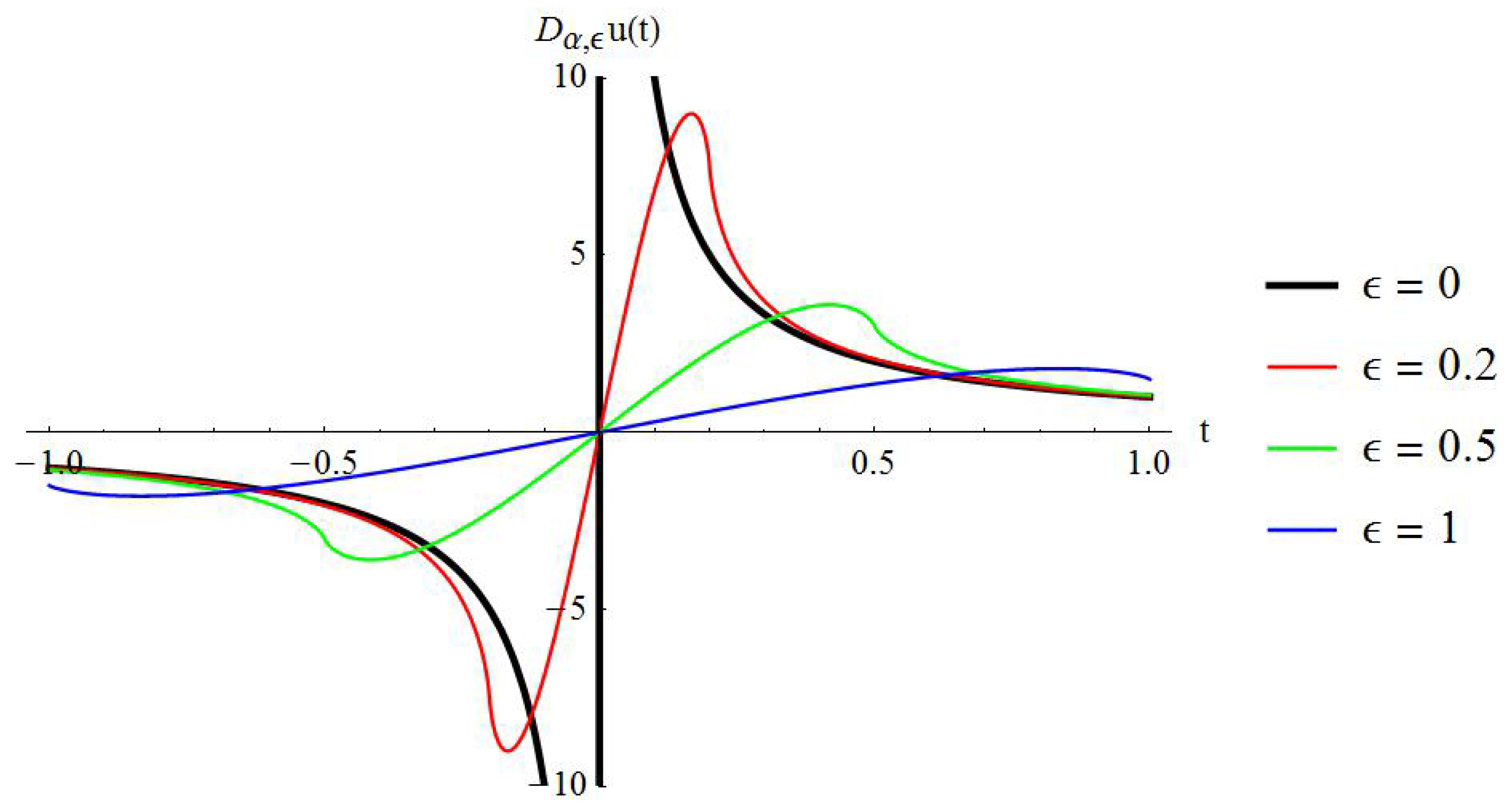
Figure 1 demonstrates that this convergence also occurs for functions that are not continuous everywhere. In this computation, we used the kernel $\alpha \left(s\right)=s{\mathbb{1}}_{(-1,1)}\left(s\right)$ and applied it to the function $u\left(t\right)=ln\left|t\right|$.

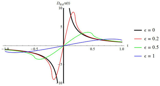
Figure 1. $D_{\alpha ,ϵ}u\left(t\right)$ for $u\left(t\right)=ln\left|t\right|$ and $\alpha \left(s\right)=s{\mathbb{1}}_{(-1,1)}$(s).

We note that the anti-symmetry condition (7) is critical for interpreting $D_{\alpha ,ϵ}$ as an extension of the classical derivative $d/dt$, or as a “first order” operator, as evident from its role in (8). Symmetric kernels ${\alpha }_{ϵ}$ would instead give something similar to a “second order” operator like $d^2/d{t}^2$; indeed, convergence to such for a similar integral operator was proven in [13].

For simplicity, we consider integrable kernels (for non-integrable kernels used in related contexts, see [14]):

$$\begin{array}{c}\hfill {\parallel \alpha \parallel }_{L^1}={\int }_{\mathbb{R}}\left|\alpha \left(s\right)\right|\mathrm{d}s<\infty .\end{array}$$

(9)

3. Initial Volume Problems

We now formulate non-local initial value problems. Because the operator G in (4) acts nonlocally, we must formulate initial data for such a problem on an interval rather than on a point. We are thus led to the notion of an initial volume problem, for which we specify u on a time interval of nonzero measure (volume). This type of problem can be thought of as a one-sided volume-constrained problem [3] analogously to the relationship between initial value problems and boundary-value problems.

We consider a formulation for an initial value problem that, in general, fails to have function-valued solutions. In general, the solutions are distributions with support at isolated (and $ϵ$-periodic) points. On the other hand, the non-singular parts of the solutions can be $C^{\infty }$. We demonstrate using some exact solutions that, in fact, these smooth parts of the solutions converge to the classical solution as $ϵ\to 0$.

3.1. Formulation

Suppose that ${\alpha }_{ϵ}$ satisfies conditions (5)–(7) and (9), such that it is supported in $(-ϵ,ϵ)$. Given a fixed horizon parameter $ϵ$, we consider compact intervals ${\Gamma }_{-}=[t_0-2ϵ,t_0]$, $\Omega =[t_0,t_N]$, and ${\Gamma }_{+}=[t_N,t_N+ϵ]$ with $t_N=t_0+Nϵ$ for some integer $N\ge 0$. (The integer is taken for convenience without loss of generality, since, if we did not have an integral domain, then we could solve our equation on a larger integral domain and restrict our solution to the original domain.) We call $\Gamma ={\Gamma }_{-}\cup {\Gamma }_{+}$ the “collar” and $\Omega$ the “body”. In peridynamics, for example, the latter is where the physical process takes place, while the former provides necessary information needed by the nonlocal interactions in the body. In this setting, we regard ${\Gamma }_{-}$ as an interval of time that initial data is defined on and ${\Gamma }_{+}$ as an auxiliary “cut-off” set of time on which no data or equation is prescribed. Observe that the width of the collar vanishes as $ϵ\to 0$, since $\Gamma \to \{t_0,\}$.

We say that u is a solution to the initial volume problem if:

$$\begin{array}{cc}\hfill & D_{\alpha ,ϵ}{u}_{ϵ}\left(t\right):={\int }_{t-ϵ}^{t+ϵ}\alpha (s-t)u_{ϵ}\left(s\right)\mathrm{d}s=F(t,u_{ϵ}\left(t\right)),t\in [t_{-1},t_N],\hfill \end{array}$$

(10)

$$\begin{array}{cc}\hfill & u_{ϵ}\left(t\right)=f_{ϵ}\left(t\right),t\in [t_{-2},t_0],f_{ϵ}\in C^{\infty }\left({\Gamma }_{-}\right),\hfill \end{array}$$

(11)

where F is a $C^{\infty }$ function of its arguments, ${\alpha }_{ϵ}$ is a $C^{\infty }$ kernel, and, in general, we allow $f_{ϵ}$ to depend (continuously) on $ϵ$.

Remark 1.

We essentially require that $D_{\alpha ,ϵ}{u}_{ϵ}=F$ in both the body Ω and the upper portion of the lower collar ${\Gamma }_{-}$.

Remark 2.

Letting $ϵ\to 0$ in (10)–(11) recovers the initial value problem $u^{\prime }\left(t\right)=F(t,u\left(t\right))$ subject to $u\left(t_0\right)={lim}_{ϵ\to 0}{f}_{ϵ}\left(t_0\right)$.

We assume that $f_{ϵ}$ satisfies the following compatibility condition:

$$\begin{array}{c}\hfill D_{\alpha ,ϵ}{f}_{ϵ}\left(t_{-1}\right)=F(t_{-1},f_{ϵ}\left(t_{-1}\right)).\end{array}$$

(12)

This condition is just (10) evaluated at $t=t_{-1}$. If this condition is not satisfied, then (10)–(11) has no classical solution (i.e., measurable function) $u_{ϵ}$.

We observe that there is some redundancy in Equation (10), since, for $t\in [t_{-1},t_0]$, we have $u_{ϵ}\left(t\right)=f_{ϵ}\left(t\right)$ and $F(t,u_{ϵ})=F(t,f_{ϵ})$ by (11). This redundancy represents the nonlocal connectedness of each domain, and leads us to employ the “method of steps” (see [15] for its use in delay differential equations and [16] for its application to delay Volterra integral equations).

To employ the method of steps, we partition the collar-body domain $[t_{-2},t_{N+1}]=[t_0-2ϵ,t_0+(N+1)ϵ]$ into $N+3$ intervals (steps) $I_n=[t_{n-1},t_n]$, where $t_n=t_0+nϵ,-2\le n\le N+1$. We define $u_{ϵ}\left(t\right)=u_n\left(t\right)$ if $t\in I_n$ as well as $u_{\left(n\right)}\left(t\right)=u_m\left(t\right)$ if $t\in I_m$ for $-1\le m\le n$, so that the problem (10)–(11) splits into:

$$\begin{array}{c}\hfill \begin{array}{cc}\hfill & {\int }_{t_n}^{t+ϵ}\alpha (s-t)u_{n+1}\left(s\right)\mathrm{d}s=\hfill \\ \hfill & F(t,u_{\left(n\right)}\left(t\right))-{\int }_{t-ϵ}^{t_n}\alpha (s-t)u_{\left(n\right)}\left(s\right)\mathrm{d}s,t\in I_n,0\le n\le N,\hfill \end{array}\end{array}$$

(13)

where $u_{\left(0\right)}=f_{ϵ}$ by (11).

We qualitatively describe how to understand solutions of this system. Because $u_{\left(0\right)}\left(x\right)=f_{ϵ}\left(x\right)$ is a known quantity, we interpret (13) for $n=0$ as a stand-alone equation to be solved for $u_1\left(x\right)$. In the solving of this equation, we claim that this equation is “decoupled” from the others in (13) and may be solved independently. So, once we find $u_1$ from this equation, we can set $n=1$ in (13) and solve for $u_2$, given that $u_{\left(1\right)}$ is now a known function. Proceeding in this way until $n=N$, we can find $u_{N+1}$ in terms of the known function $u_{\left(N\right)}$. Observe how this “iterative” procedure is similar to the finite difference numerical solution of an initial value problem.

The solutions of this system can be found using Laplace transforms. This can be verified symbolically on computer algebra systems, such as Mathematica or Maple, provided the kernel $\alpha \left(t\right)$ and source term $F(t,u)$ are specified.

3.2. Exact Solutions

We illustrate some general features of the initial volume problem (10)–(11) by solving some simple problems exactly, emphasizing similarities and differences between these solutions and their classical counterparts. We highlight that each nonlocal solution is singular at $ϵ$-periodic intervals and that these solutions converge to the classical solutions as $ϵ\to 0$.

3.2.1. The Equation $u^{\prime }\left(t\right)=1$ with $u\left(0\right)=0$

Let us consider the classical initial value problem $u^{\prime }\left(t\right)=1$ subject to $u\left(0\right)=0$. Obviously, the solution to this problem is $u\left(t\right)=t$. We investigate a nonlocal extension of this problem:

$$\begin{array}{c}\hfill \begin{array}{cc}\hfill & D_{\alpha ,ϵ}{u}_{ϵ}\left(t\right)=1,-ϵ\le t,\hfill \\ \hfill & u_{ϵ}\left(t\right)=(1+2ϵ)t+t^2,-2ϵ\le t\le 0.\hfill \end{array}\end{array}$$

(14)

We choose ${\alpha }_{ϵ}\left(s\right)=3s/\left(2{ϵ}^3\right){\mathbb{1}}_{(-ϵ,ϵ)}\left(s\right)$ as our kernel, since it is both simple for computations as well as $C^{\infty }$ on its support. We solve for $u_{ϵ}$ on $[t_{-2},t_{N+1}]=[-2ϵ,1+ϵ]$.

We chose the initial condition $f_{ϵ}\left(t\right)=(1+2ϵ)t+t^2$ so that Equation (13) holds at $t=t_{-1}=-ϵ$ for $n=0$. If our function $f_{ϵ}$ did not satisfy this condition, then our problem (10)–(11) would be ill-posed in the space of measurable functions, and we would instead need to consider distribution solutions. Observe that $u_{ϵ}\left(0\right)=0$, so that this initial condition agrees with its classical counterpart $u\left(0\right)=0$. In general, we could choose it to agree only at $\mathcal{O}\left(ϵ\right)$.

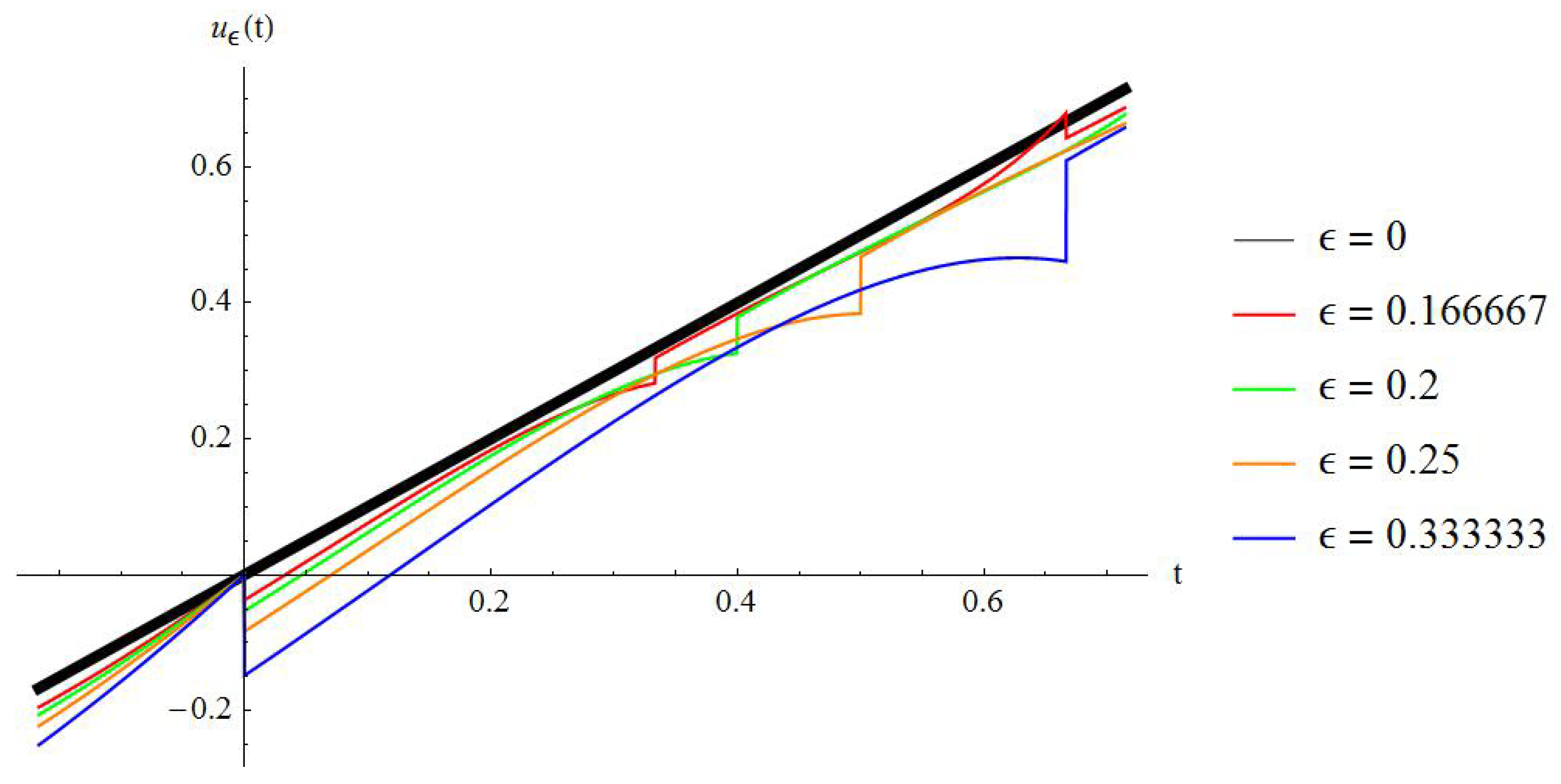
Using Laplace transforms to solve the system (13), we find that the exact solution to (14) is given by the following piecewise sequence:

$$\begin{array}{c}\hfill \begin{array}{cc}\hfill & u_0\left(t\right)=(1+2ϵ)t+t^2,-2ϵ\le t<0,\hfill \\ \hfill & u_1\left(t\right)=u_0\left(t\right)-{\displaystyle \frac{4{ϵ}^2}{3}}{e}^{t/ϵ},0<t<ϵ,\hfill \\ \hfill & u_2\left(t\right)=u_1\left(t\right),ϵ<t<2ϵ,\hfill \\ \hfill & u_3\left(t\right)=u_1\left(t\right)+{\displaystyle \frac{4ϵ}{3}}{e}^{t/ϵ-2}(2t-3ϵ),2ϵ<t<3ϵ,\hfill \\ \hfill & u_4\left(t\right)=u_3\left(t\right),3ϵ<t<4ϵ,\hfill \\ \hfill & ⋮\hfill \end{array}\end{array}$$

(15)

In Figure 2, we plot $u_{ϵ}\left(t\right)$ in (15) on $[0,1]$ next to $u\left(t\right)=t$ for different values of $ϵ$. There are several things to observe. First, each function $u_{ϵ}$ has a noticeable discontinuity at each $t_{2n}=2nϵ$ for $n\ge 0$. Because our nonlocal initial value problem (10)–(11) does not involve classical derivatives, this lack of differentiability is unsurprising. In addition, as we take $ϵ\to 0$, we see that the functions $u_{ϵ}$ visibly converge to the classical solution u. Their convergence is only in the maximum norm or $L^{\infty }$ sense, since the periodic discontinuities persist for even the smallest $ϵ$ values.

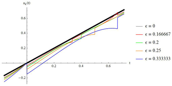
Figure 2. Solution (15) for various choices of $ϵ$. $ϵ=0$ corresponds to $u\left(t\right)=t$.

3.2.2. The Equation $u^{\prime }\left(t\right)=u\left(t\right)$ with $u\left(0\right)=1$

Let us now consider the classical initial value problem $u^{\prime }\left(t\right)=u\left(t\right)$ subject to $u\left(0\right)=1$. The classical solution to this problem is $u\left(t\right)=exp\left(t\right)$. We investigate a nonlocal extension of this problem:

$$\begin{array}{c}\hfill \begin{array}{cc}\hfill & D_{\alpha ,ϵ}{u}_{ϵ}\left(t\right)=u_{ϵ}\left(t\right),-ϵ\le t,\hfill \\ \hfill & u_{ϵ}\left(t\right)=t+ϵ+1,-2ϵ\le t\le 0,\hfill \end{array}\end{array}$$

(16)

We again choose ${\alpha }_{ϵ}\left(s\right)=3s/\left(2{ϵ}^3\right){\mathbb{1}}_{(-ϵ,ϵ)}\left(s\right)$ as our kernel and $f_{ϵ}$ so that (13) is satisfied at $t=-ϵ$ for $n=0$.

Using Laplace transforms, we find that the exact solution $u_{ϵ}$ to (16) is given by the following piecewise sequence of distributions:

$$\begin{array}{c}\hfill \begin{array}{cc}\hfill u_0\left(t\right)& =1+t+ϵ,t\in [-2ϵ,0],\hfill \\ \hfill u_1\left(t\right)& =u_0\left(t\right)+{\displaystyle \frac{2{ϵ}^2}{3}}{e}^{t/ϵ},t\in [0,ϵ)\hfill \\ \hfill u_2\left(t\right)& =u_1\left(t\right)+{\displaystyle \frac{4{ϵ}^2}{9}}{e}^{t/ϵ-1}(t+ϵ)+{\displaystyle \frac{4{ϵ}^3}{9}}{\delta }_{ϵ}(t/ϵ),t\in (ϵ,2ϵ)\hfill \\ \hfill u_3\left(t\right)& =u_2\left(t\right)+\dots +{\displaystyle \frac{8}{9}}{ϵ}^4{\delta }_{2ϵ}(t/ϵ)+{\displaystyle \frac{8}{27}}{ϵ}^4{\delta }_{2ϵ}^{\prime }(t/ϵ),t\in (2ϵ,3ϵ),\hfill \\ \hfill & ⋮\hfill \end{array}\end{array}$$

(17)

where the ellipses denote non-singular functions.

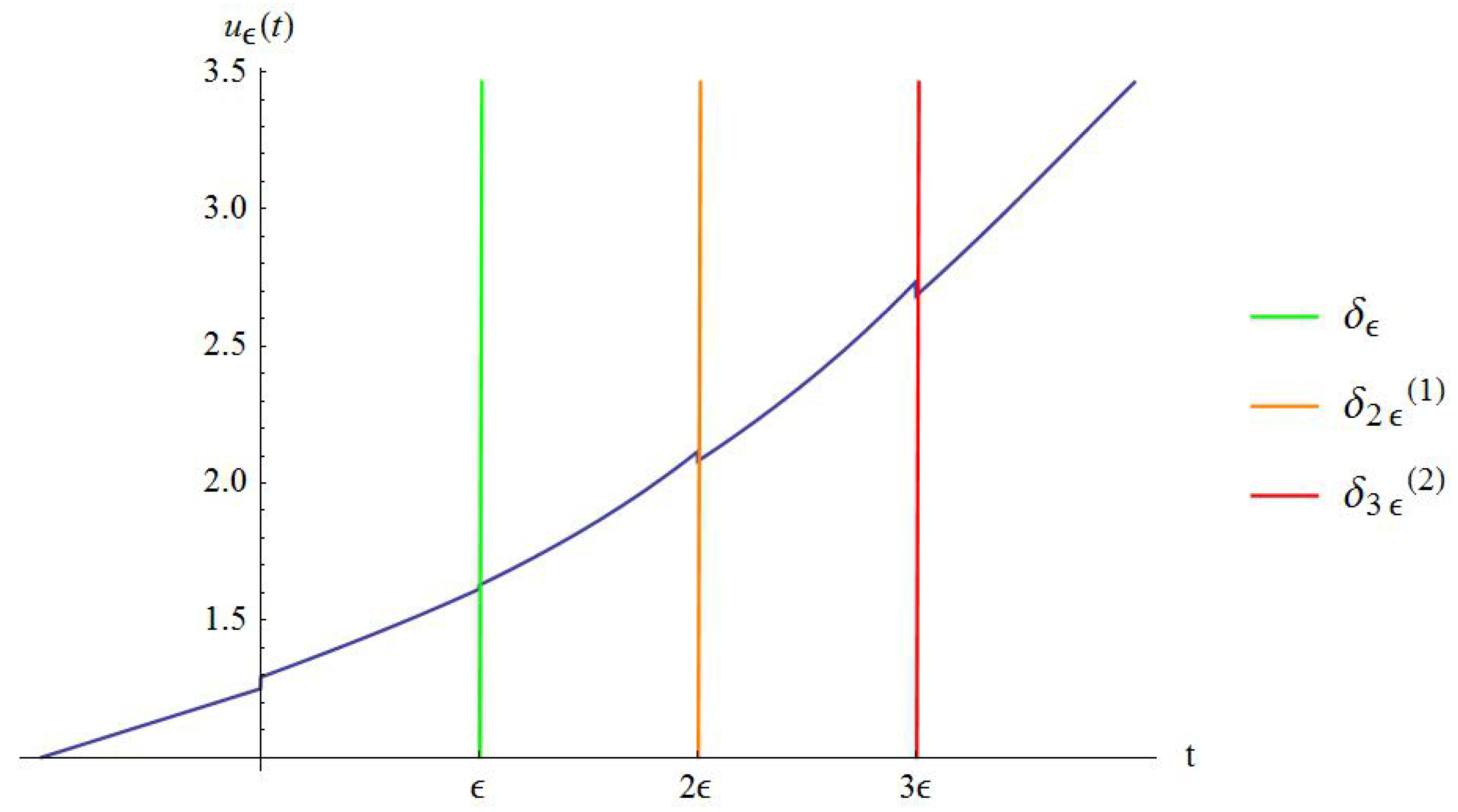
We plot $u_{ϵ}$ in Figure 3 for $ϵ=1/4$. In contrast to the solution (15), we see that (17) develops a distribution-valued singularity at $t=ϵ$. This shows that the initially well-posed problem (16) no longer has a function-valued solution once we reach this time. In other words, $u_{ϵ}$ “blows up” at $t=ϵ$. In fact, the order of the distribution’s singularity increases with time (e.g., $u_4$ contains a ${\delta }_{3ϵ}^{″}(t/ϵ)$ term). Finite-time blowup is a typically nonlinear phenomenon, but we see that the linear problem (16) exhibits this as well.

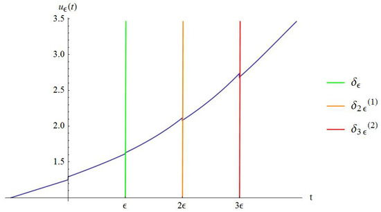
Figure 3. Solution (17) for $ϵ=1/4$. Vertical lines indicate locations of singularities.

Another interesting feature is that the functions $u_n$ are each $C^{\infty }$ on the open intervals $(t_{n-1},t_n)$. The high degree of regularity is due to that of $f_{ϵ}$ and $F(t,u)$, but the fact remains that the distributional singularities are confined to the points $t_m=ϵm$ for $m\ge 1$.

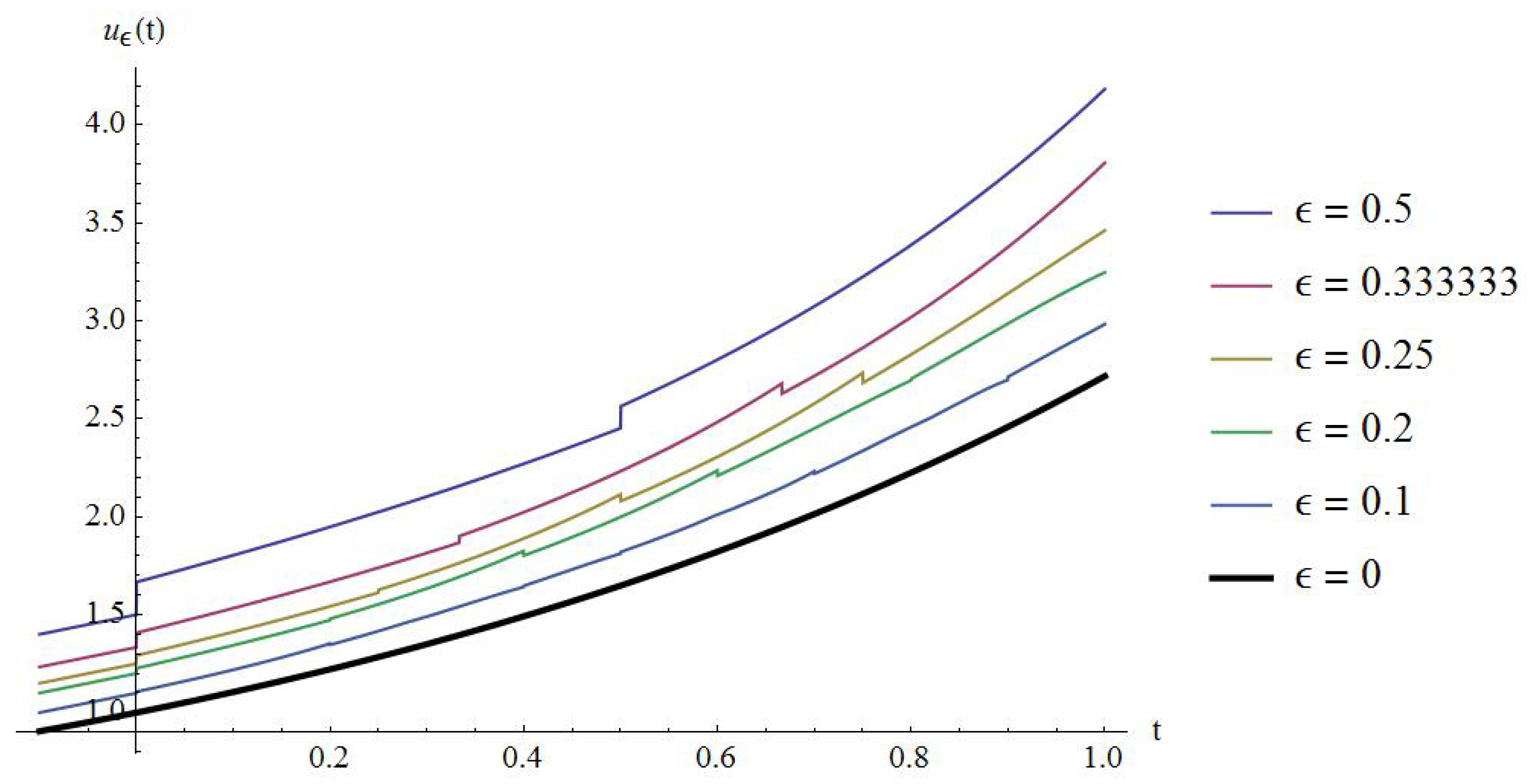
Finally, we observe that each ${\delta }_0$ term in (17) has a coefficient of high degree in $ϵ$. This shows that each distributional singularity in $u_{ϵ}$ vanishes as $ϵ\to 0$ (in the weak sense). Moreover, from Figure 4, we see that the $C^{\infty }$ parts of the solution $u_{ϵ}$ converge to the classical solution $u\left(t\right)=e^t$. Thus, although the nonlocal solution $u_{ϵ}$, being distribution-valued, differs greatly from its classical counterpart, it still recovers the latter in the classical limit.

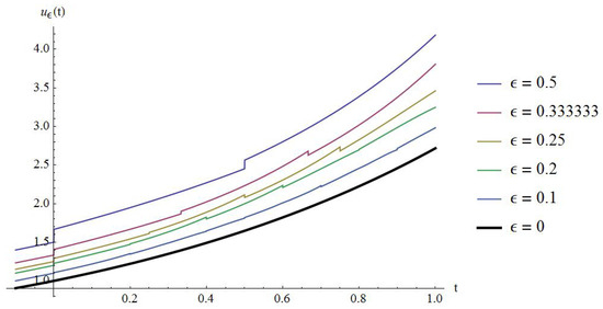
Figure 4. Solution (17) for various choices of $ϵ$; $ϵ=0$ corresponds to $u\left(t\right)=e^t$.

3.3. Connections with Volterra Integral Equations

Many of the mathematical features seen for the exact solutions (15) and (17) of the initial volume problems (14) and (16) can be explained by recasting the system (13) as a set of linear Volterra integral equations of the first kind. Such an integral equation has the following form:

$$\begin{array}{c}\hfill {\int }_a^{x}K(x-y)v\left(y\right)\mathrm{d}y=g\left(x\right),a<x<b,\end{array}$$

(18)

where v is the function to be solved for on $[a,b]$, and $K:[0,b-a]\to \mathbb{R}$ is the kernel.

We can put each equation of the system (13) into the form of (18) as follows. For $0\le n\le N$, set $a=x_{n-1}$, $b=x_n$, $K\left(z\right)=-\alpha (z-ϵ),0\le z\le ϵ$, $v\left(x\right)=u_{n+1}(x+ϵ)$, and $g\left(x\right)$ equal to the right hand side of (13).

Ultimately, the singularities we have seen for the solutions of (13) stem from the wellposedness properties of (18). The problem (18) does not always admit a function-valued solution. If g in (18) is continuous on $[a,b]$, then letting $x\to a$ in (18) shows that either $g\left(a\right)$ is zero, or there is no integrable function v that solves (18). However, as shown in [17], even if $g\left(a\right)\ne 0$, we can still find generalized solutions (i.e., distributions) to (18). Essentially, including these distributional singularities in v “compensates” for $g\left(a\right)\ne 0$ by adding an extra contribution to the integral in (18).

We can now show why the initial volume problem (16) admits only generalized solutions and why the problem (14) admits classical ones. Let us find the conditions analogous to $g\left(a\right)=0$ in (18) necessary for (13) to admit classical solutions. For some $n\ge 0$, we set $t=t_{n-1}$ in (13):

$$\begin{array}{c}\hfill 0=F(t_{n-1},u_{\left(n\right)}\left(t_{n-1}\right))-{\int }_{t_{n-2}}^{t_n}\alpha (s-t_{n-1})u_{\left(n\right)}\left(s\right)\mathrm{d}s.\end{array}$$

We can refine this expression by considering (13) for $n-1$ and setting $t=t_{n-1}$:

$$\begin{array}{c}\hfill {\int }_{t_{n-1}}^{t_n}\alpha (s-t_{n-1})u_n\left(s\right)\mathrm{d}s=F(t_{n-1},u_{(n-1)}\left(t_{n-1}\right))-{\int }_{t_{n-2}}^{t_{n-1}}\alpha (s-t_{n-1})u_{(n-1)}\left(s\right)\mathrm{d}s.\end{array}$$

Subtracting these two expressions gives the compatibility conditions necessary for classical solutions of (13) (assuming that (12) is satisfied):

$$\begin{array}{c}\hfill F(t_{n-1},u_{n-1}\left(t_{n-1}\right))=F(t_{n-1},u_n\left(t_{n-1}\right)),0\le n\le N.\end{array}$$

(19)

For problem (14), we have $F\equiv 1$, so it is clear that condition (19) is satisfied. This shows why the solution (15) is classical. On the other hand, for problem (16), we have $F(t,u)=u$, so condition (19) becomes $u_{n-1}\left(t_{n-1}\right)=u_n\left(t_{n-1}\right),0\le n\le N$. In essence, this condition requires the continuity of u over the entire domain $[t_{-2},t_{N+1}]$, rather than simply on each interval $(t_{n-1},t_n)$. From Figure 4, we see that this is not the case. Even at $t=0$, where the solution is classical, the solution jumps up from its initial condition $u_0\left(0\right)=1+ϵ$ to $u_1\left(0\right)=1+ϵ+2{ϵ}^2/3$. The failure of condition (19) at $t=0$ gives rise to the singularity at $t=ϵ$.

We now connect the failure of (19) to the classical situation (i.e., $ϵ=0$). Differentiating (13) and setting $n=0$:

$$\begin{array}{c}\hfill {\alpha }_{ϵ}\left(ϵ\right)u_1(t+ϵ)-{\int }_{ϵ}^{t+ϵ}{\alpha }^{\prime }(s-t)u_1\left(s\right)\mathrm{d}s=F_t+f_{ϵ}^{\prime }\left(t\right)F_u-{\alpha }_{ϵ}\left(ϵ\right)f_{ϵ}(t-ϵ)\\ \hfill +{\int }_{t-ϵ}^0{\alpha }_{ϵ}^{\prime }(s-t)f_{ϵ}\left(s\right)\mathrm{d}s.\end{array}$$

[We have converted the first kind Volterra Equation (18) into a second kind Volterra equation, see, e.g., [18]]. Setting $t=-ϵ$ in this expression:

$$\begin{array}{c}\hfill {\alpha }_{ϵ}\left(ϵ\right)u_1\left(0\right)=F_t(-ϵ,f_{ϵ}(-ϵ))+f_{ϵ}^{\prime }(-ϵ)F_u(-ϵ,f_{ϵ}(-ϵ))-{\alpha }_{ϵ}\left(ϵ\right)f_{ϵ}(-2ϵ)+{\int }_{-2ϵ}^0{\alpha }_{ϵ}^{\prime }(s+ϵ)f_{ϵ}\left(s\right)\mathrm{d}s.\end{array}$$

Integrating the last term by parts and rearranging, we obtain a condition on the first “jump” of $u_{ϵ}$:

$$\begin{array}{c}\hfill u_1\left(0\right)-f_{ϵ}\left(0\right)={\displaystyle \frac{1}{{\alpha }_{ϵ}\left(ϵ\right)}}\left[F_t(-ϵ,f_{ϵ}(-ϵ))+f_{ϵ}^{\prime }(-ϵ)F_u(-ϵ,f_{ϵ}(-ϵ))-{\int }_{-2ϵ}^0{\alpha }_{ϵ}(s+ϵ)f_{ϵ}^{\prime }\left(s\right)\mathrm{d}s\right],\end{array}$$

(20)

where we assumed that ${\alpha }_{ϵ}\left(ϵ\right)\ne 0$ without loss of generality (since we could differentiate again and instead consider ${\alpha }_{ϵ}^{\prime }\left(ϵ\right)$).

Since we have $1/{\alpha }_{ϵ}\left(ϵ\right)={ϵ}^2{\int }_{-1}^{1}s\alpha \left(s\right)\mathrm{d}s/\alpha \left(1\right)$ by (5), we conclude that the jump discontinuity of $u_{ϵ}$ is of $\mathcal{O}\left({ϵ}^2\right)$. Therefore, in the classical limit, the jump discontinuities in $u_{ϵ}$ vanish, which means that the compatibility condition (19) is satisfied in this limit. This shows that the distribution singularities that “compensate” for the failure of (19) actually disappear in the classical limit. Of course, we expected this, since the classical solutions to $u^{\prime }\left(t\right)=u\left(t\right)$ are all smooth.

3.4. Connections with Functional Differential Equations

We show that (10) is closely related to so-called “advance/delay ODEs”. Consider ${\alpha }_{ϵ}\left(s\right)=Cs$, where $C=3/\left(2{ϵ}^3\right)$, and, for simplicity, let $F(t,u)=u$. Differentiating (10) gives:

$$\begin{array}{c}\hfill Cϵ(u_{ϵ}(t+ϵ)-u_{ϵ}(t-ϵ))-C{\int }_{t-ϵ}^{t+ϵ}{u}_{ϵ}\left(s\right)\mathrm{d}s=u_{ϵ}^{\prime }\left(t\right).\end{array}$$

Differentiating this again:

$$\begin{array}{c}\hfill Cϵ(u_{ϵ}^{\prime }(t+ϵ)-C{u}_{ϵ}^{\prime }(t-ϵ))-(u_{ϵ}(t+ϵ)-u_{ϵ}(t-ϵ))=u_{ϵ}^{″}\left(t\right).\end{array}$$

(21)

This is an example of a second-order advance/delay ODE, since the highest order derivative $u_{ϵ}^{″}\left(t\right)$ appears in the same equation as the delayed terms $u_{ϵ}(t-ϵ)$ and $u_{ϵ}^{\prime }(t-ϵ)$ and the advanced terms $u_{ϵ}(t+ϵ)$ and $u_{ϵ}^{\prime }(t+ϵ)$. Another name commonly used in the literature is “functional differential equation of mixed type” [19]. In general, for polynomial kernels ${\alpha }_{ϵ}$ of degree n, the integral equation (10) is equivalent to an advanced/delay ODE of order $n+1$. We may call (10) an “advance/delay integral equation”.

Delay ODEs show up very frequently in practical applications, but advanced ODEs and advanced integral equations (IEs) have been studied much less. Some applications for advanced ODEs are in electromagnetic theory [20], modeling tsunami rogue waves [21], nerve conduction [22], and traveling waves in lattice domains [23]. Advanced or mixed type IEs have appeared in endogenous growth models with vintage capital [24] and storage size optimization [25]. Driver [26] studied wellposedness for some mixed-type ODEs in the context of an initial value problem, and Oztepe and Bereketoglu [27] studied that for an advanced-impulsive ODE, but most authors have studied advanced ODEs from boundary value problem perspectives [28] or based on asymptotic behavior at infinity [29,30,31,32].

One reason for this lack of investigation for initial value problems is that such problems for advanced ODEs can be ill-posed in the usual function spaces [23,33,34]. One heuristic reason for this ill-posedness is as follows. In general, we do not know the future in a very precise way. We may have some vague impressions, but most of what we know is educated guesswork. Therefore, if we try to make decisions in the present based on very precise information needed from future events, we will often run into problems.

This is precisely the type of situation occurring in the advance/delay integral equation (10) and the advance/delay ODE (21): the present value of the function $u_{ϵ}$ is being influenced by both its past and future values via the nonlocal derivative $D_{\alpha ,ϵ}$. Based on these heuristic ideas, it is not too surprising that these problems are, in general, ill-posed. However, what we have shown is that these futuristic equations still admit generalized solutions, so there may still be some way to interpret both these solutions as well as the idea of the future influencing the present.

4. Final Remarks

In Section 3.2.2, we observed that solutions of the nonlocal initial volume problem developed distributional singularities with increasing time. The reason was the future information required to advance the solution further in time, rendering the problem ill posed. A surprising fact about this phenomenon is that the equation is linear. It is usually nonlinear PDEs which develop singularities in time.

It is therefore natural to ask what happens if we solve the nonlinear equation $D_{\alpha ,ϵ}{u}_{ϵ}=u_{ϵ}^2$. The classical $ϵ=0$ analogue $u^{\prime }\left(t\right)=u{\left(t\right)}^2$ has solutions which blow up in finite time, if the initial data is positive. For the nonlocal equation, the solutions again develop distributional singularities, but these later develop into products of distributions, such as ${\delta }_a^2$. Such products are not well defined as distributions. We omit the details here, but this singularity development can be shown again using the method of steps and Laplace transforms.

This suggests that nonlinearity adds an additional layer of ill-posedness to nonlocal evolution equations. It would be interesting future work to consider such effects of nonlocality on nonlinear particle interactions [35,36], which are known to have applications in physics.

Another natural direction is to study the wellposedness and numerical analysis for time evolution equations using this paper’s nonlocal operator. For nonlinear equations, such analysis of distributional singularities may require the use of Colombeau algebras. The wellposedness and numerical analysis for nonlinear convection with a spatial nonlocality was studied in [37,38].

Given the finite time singularity results for the model problems considered in the present paper, it is possible that partial differential equation models, obtained by using the nonlocal time derivative of this paper, will exhibit finite time blowup. The strength of the blowup may even be stronger than distributional, and its study would be interesting future work.

The new singularity features observed here may be of interest to develop new mathematical models. One may wish to preserve some structural aspect of a partial differential equation model, such as a conservation law, while adding in new features that partial differential equations lack because of the absence of future data. As a basic exploratory hypothesis, one area of application might be in mathematical finance, where stock market bubbles routinely form around every 10 years. In part, these bubbles are speculative, which is to say that investors collectively made an assumption about the future market behavior. When this assumption failed, the bubble collapsed, and a market singularity developed. From the perspective of the present paper, market speculation could be associated with our nonlocal time derivative operator, since it evolves the dynamics with the future in mind. The market bubbles are analogous to the periodic singularities that develop in this paper’s model systems. Of particular note is the ability to continue the dynamical system after the singularity, unlike with many nonlinear PDEs with singularities, since markets are able to recover after the bubble bursts.

References

- Marigo, A.; Piccoli, B. Regular syntheses and solutions to discontinuous ODEs. ESAIM Control Optim. Calc. Var. 2002, 7, 291–307. [Google Scholar]
- Dieci, L.; Lopez, L. A survey of numerical methods for IVPs of ODEs with discontinuous right-hand side. J. Comput. Appl. Math. 2012, 236, 3967–3991. [Google Scholar] [CrossRef]
- Du, Q.; Gunzburger, M.; Lehoucq, R.B.; Zhou, K. A Nonlocal Vector Calculus, nonlocal volume-constrained problems, and nonlocal balance laws. Math. Model. Methods Appl. Sci. 2013, 23, 493–540. [Google Scholar] [CrossRef]
- Silling, S. Reformulation of elasticity theory for discontinuities and long-range forces. J. Mech. Phys. Solids 2000, 48, 175–209. [Google Scholar] [CrossRef]
- Bobaru, F.; Duangpanya, M. The peridynamic formulation for transient heat conduction. Int. J. Heat Mass Transf. 2010, 53, 4047–4059. [Google Scholar] [CrossRef]
- Andreu-Vaillo, F.; Mazón, J.M.; Rossi, J.D.; Toledo-Melero, J.J. Nonlocal Diffusion Problems; Mathematical Surveys and Monographs; American Mathematical Society: Providence, RI, USA; Real Sociedad Matemática Española: Madrid, Spain, 2010; Volume 165, pp. xvi+256. [Google Scholar] [CrossRef]
- Gilboa, G.; Osher, S. Nonlocal Operators with Applications to Image Processing. Multiscale Model. Simul. 2009, 7, 1005–1028. [Google Scholar] [CrossRef]
- Weckner, O.; Brunk, G.; Epton, M.A.; Silling, S.A. Green’s functions in non-local three-dimensional linear elasticity. Proc. Roy. Soc. Edinb. Sect. A 2009, 465, 3463–3487. [Google Scholar] [CrossRef]
- Mengesha, T.; Du, Q. The bond-based peridynamic system with Dirichlet-type volume constraint. Proc. Roy. Soc. Edinb. Sect. A 2014, 144, 161–186. [Google Scholar] [CrossRef]
- Radu, P.; Toundykov, D.; Trageser, J. A nonlocal biharmonic operator and its connection with the classical bi-Laplacian. arXiv 2014, arXiv:1410.3488. [Google Scholar]
- Du, Q.; Kamm, J.R.; Lehoucq, R.B.; Parks, M.L. A new approach for a nonlocal, nonlinear conservation law. SIAM J. Appl. Math. 2012, 72, 464–487. [Google Scholar] [CrossRef]
- Heymans, N.; Podlubny, I. Physical interpretation of initial conditions for fractional differential equations with Riemann-Liouville fractional derivatives. Rheol. Acta 2006, 45, 765–771. [Google Scholar] [CrossRef]
- Du, Q.; Zhou, K. Mathematical analysis for the peridynamic nonlocal continuum theory. ESAIM Math. Model. Numer. Anal. 2011, 45, 217–234. [Google Scholar]
- Du, Q.; Gunzburger, M.; Lehoucq, R.B.; Zhou, K. Analysis and approximation of nonlocal diffusion problems with volume constraints. SIAM Rev. 2012, 54, 667–696. [Google Scholar] [CrossRef]
- Baker, C.T.; Paul, C.A.; Willé, D.R. Issues in the numerical solution of evolutionary delay differential equations. Adv. Comput. Math. 1995, 3, 171–196. [Google Scholar]
- Brunner, H. The numerical analysis of functional integral and integro-differential equations of Volterra type. Acta Numer. 2004, 13, 55–145. [Google Scholar]
- Sidorov, N.A.; Sidorov, D.N. Existence and construction of generalized solutions of nonlinear Volterra integral equations of the first kind. Differ. Equ. 2006, 42, 1312–1316. [Google Scholar]
- Polyanin, A.D.; Manzhirov, A.V. Handbook of Integral Equations; CRC Press: Boca Raton, FL, USA, 2008; p. 796. [Google Scholar]
- Rustichini, A. Functional differential equations of mixed type: The linear autonomous case. J. Dyn. Differ. Equ. 1989, 1, 121–143. [Google Scholar]
- Schulman, L.S. Some differential difference equations containing both advance and retardation. J. Math. Phys. 1974, 15, 295–298. [Google Scholar]
- Pravica, D.W.; Randriampiry, N.; Spurr, M.J. q-Advanced Models for Tsunami and Rogue Waves. Abstr. Appl. Anal. 2012, 2012, 414060. [Google Scholar]
- Chi, H.; Bell, J.; Hassard, B. Numerical solution of a nonlinear advance-delay-differential equation from nerve conduction theory. J. Math. Biol. 1986, 24, 583–601. [Google Scholar]
- Härterich, J.; Sandstede, B.; Scheel, A. Exponential dichotomies for linear nonautonomous functional differential equations of mixed type. Indiana Univ. Math. J. 2002, 51, 1081–1109. [Google Scholar]
- Boucekkine, R.; Licandro, O.; Puch, L.A.; Rio, F.D. Vintage capital and the dynamics of the AK model. J. Econom. Theory 2005, 120, 39–72. [Google Scholar]
- Orbán-Mihálykó, É.; Lakatos, B.G. On the advanced integral and differential equations of the sizing procedure of storage devices. Funct. Differ. Equ. 2004, 11, 121–132. [Google Scholar]
- Driver, R.D. A mixed neutral system. Nonlinear Anal. 1984, 8, 155–158. [Google Scholar]
- Oztepe, G.S.; Berkeketoglu, H. Convergence in an impulsive advanced differential equations with piecewise constant argument. Bull. Math. Anal. Appl. 2012, 4, 57–70. [Google Scholar]
- Jankowski, T. Advanced differential equations with nonlinear boundary conditions. J. Math. Anal. Appl. 2005, 304, 490–503. [Google Scholar]
- Diblik, J. A note on explicit criteria for the existence of positive solutions to the linear advanced equation. Appl. Math. Lett. 2014, 35, 72–76. [Google Scholar]
- Hupkes, H.J.; Augeraud-Véron, E. Well-posedness of initial value problems for functional differential and algebraic equations of mixed type. Discret. Contin. Dyn. Syst. 2011, 30, 737–765. [Google Scholar]
- Yi-zhong, L. The bounded solution of a class of differential-difference equation of advanced type and its asymptotic behavior. Appl. Math. Mech. (Engl. Ed.) 1988, 9, 579–586. [Google Scholar]
- Trench, W.F. Existence and nonoscillation theorems for an Emden-Fowler equation with deviating argument. Trans. Am. Math. Soc. 1986, 294, 217–231. [Google Scholar]
- Kato, T. The functional differential equation y’(x) = ay (Ax)+ by (x). Delay Funct. Differ. Equ. Appl. 2014, 197. [Google Scholar]
- Wiener, J. Generalized Solutions of Functional Differential Equations; World Scientific: Singapore, 1993; p. 410. [Google Scholar]
- Liang, Z.X.; Zhang, Z.D.; Liu, W.M. Dynamics of a Bright Soliton in Bose-Einstein Condensates with Time-Dependent Atomic Scattering Length in an Expulsive Parabolic Potential. Phys. Rev. Lett. 2005, 94, 050402. [Google Scholar] [PubMed]
- Ji, A.C.; Liu, W.M.; Song, J.L.; Zhou, F. Dynamical Creation of Fractionalized Vortices and Vortex Lattices. Phys. Rev. Lett. 2008, 101, 010402. [Google Scholar] [PubMed]
- Du, Q.; Huang, Z.; LeFloch, P.G. Nonlocal conservation laws. A new class of monotonicity-preserving models. SIAM J. Numer. Anal. 2017, 55, 2465–2489. [Google Scholar]
- Huang, K.; Du, Q. Asymptotic Compatibility of a Class of Numerical Schemes for a Nonlocal Traffic Flow Model. SIAM J. Numer. Anal. 2024, 62, 1119–1144. [Google Scholar]
Disclaimer/Publisher’s Note: The statements, opinions and data contained in all publications are solely those of the individual author(s) and contributor(s) and not of MDPI and/or the editor(s). MDPI and/or the editor(s) disclaim responsibility for any injury to people or property resulting from any ideas, methods, instructions or products referred to in the content. |
© 2024 by the author. Licensee MDPI, Basel, Switzerland. This article is an open access article distributed under the terms and conditions of the Creative Commons Attribution (CC BY) license (https://creativecommons.org/licenses/by/4.0/).