Stationary Distribution and Density Function for a High-Dimensional Stochastic SIS Epidemic Model with Mean-Reverting Stochastic Process

Abstract

This paper explores a high-dimensional stochastic SIS epidemic model characterized by a mean-reverting, stochastic process. Firstly, we establish the existence and uniqueness of a global solution to the stochastic system. Additionally, by constructing a series of appropriate Lyapunov functions, we confirm the presence of a stationary distribution of the solution under $R_0^s>1$. Taking 3D as an example, we analyze the local stability of the endemic equilibrium in the stochastic SIS epidemic model. We introduce a quasi-endemic equilibrium associated with the endemic equilibrium of the deterministic system. The exact probability density function around the quasi-stable equilibrium is determined by solving the corresponding Fokker–Planck equation. Finally, we conduct several numerical simulations and parameter analyses to demonstrate the theoretical findings and elucidate the impact of stochastic perturbations on disease transmission.

1. Introduction

According to data from the United Nations AIDS Programme, approximately 38 million individuals worldwide are infected with the AIDS virus, with around 6.9 million of them not receiving HIV treatment post-infection, and about 1.5 million succumbing to AIDS or AIDS-related illnesses annually. Particularly in Africa, AIDS has emerged as a critical public health concern. In numerous countries, the prevalence of AIDS infections is alarmingly high, significantly impacting local socioeconomic progress and public health [1]. The epidemiological examination of AIDS and the comprehensive elucidation by Hyman et al. delineate that AIDS infection progresses through three phases. Despite this, effective vaccines or treatments for AIDS patients are yet to be developed. Mathematical modeling aids in comprehending the transmission of HIV/AIDS [2,3,4,5,6,7,8,9]. Notably, a standard ODE model has been devised to depict the disease’s dissemination based on its characteristics [9,10].

$$\left\{\begin{array}{c}{\displaystyle \frac{dS\left(t\right)}{dt}}=\mu (S\left(0\right)-S\left(t\right))-{\displaystyle \frac{\lambda S\left(t\right)I\left(t\right)}{N\left(t\right)}}\hfill \\ {\displaystyle \frac{dI\left(t\right)}{dt}}={\displaystyle \frac{\lambda S\left(t\right)I\left(t\right)}{N\left(t\right)}}-(\mu +\gamma )I\left(t\right)\hfill \\ {\displaystyle \frac{dA\left(t\right)}{dt}}=\gamma I\left(t\right)-\delta A\left(t\right)\hfill \end{array}\right..$$

The model assumes that all constant rates (as in Table 1) are positive. Meanwhile, Hyman and Li [9] divided the susceptible people into n subgroups according to the susceptibility of each group of individuals and established the high-dimensional stochastic SIS epidemic model (differential susceptibility epidemic model) as follows:

$$\left\{\begin{array}{c}{\displaystyle \frac{d{S}_i\left(t\right)}{dt}}=\mu (S_i\left(0\right)-S_i\left(t\right))-{\displaystyle \frac{{\lambda }_i{S}_i\left(t\right)I\left(t\right)}{N\left(t\right)}},1\le i\le n\hfill \\ {\displaystyle \frac{dI\left(t\right)}{dt}}={\displaystyle \sum _{i=1}^n}{\displaystyle \frac{{\lambda }_i{S}_i\left(t\right)I\left(t\right)}{N\left(t\right)}}-(\mu +\gamma )I\left(t\right)\hfill \\ {\displaystyle \frac{dA\left(t\right)}{dt}}=\gamma I\left(t\right)-\delta A\left(t\right)\hfill \end{array}\right.,$$

(1)

where $N\left(t\right)={\displaystyle \sum _{i=1}^n}{S}_i\left(t\right)+I\left(t\right)$. The ODE models assume that all susceptible people are in the same situation and have the same degree of susceptibility, which ignores the random interaction between people. Since the group $A\left(t\right)$ of AIDS patients has no effect on the overall dynamic properties of the model, the model does not take group $A\left(t\right)$ into account [11,12], and the high-dimensional SIS model is obtained as follows:

$$\left\{\begin{array}{c}{\displaystyle \frac{d{S}_i\left(t\right)}{dt}}=\mu (S_i\left(0\right)-S_i\left(t\right))-{\displaystyle \frac{{\lambda }_i{S}_i\left(t\right)I\left(t\right)}{N\left(t\right)}},1\le i\le n\hfill \\ {\displaystyle \frac{dI\left(t\right)}{dt}}={\displaystyle {\displaystyle \sum _{i=1}^n}}{\displaystyle \frac{{\lambda }_i{S}_i\left(t\right)I\left(t\right)}{N\left(t\right)}}-(\mu +\gamma )I\left(t\right)\hfill \end{array}\right.,$$

Table 1. The definitions of the parameters.

Parameter	Definition
$S\left(t\right)$	mature people who have not been exposed to the virus
$I\left(t\right)$	mature individuals who have been infected with the virus but have not yet developed
$A\left(t\right)$	mature people developed into fully symptomatic AIDS
$N\left(t\right)$	the total of the adult population and the sexual interaction population
$\lambda$	the effective contact rate of infected persons to susceptible persons
$\mu$	natural mortality rate
$\gamma$	develop into AIDS rate
$\delta$	the mortality rate of AIDS

Notably, the mean-reverting stochastic process (Ornstein–Uhlenbeck process), with appropriate adjustments, finds application in stochastically modeling interest rates, currency exchange rates, and commodity prices [13,14,15,16,17,18,19,20]. Researchers have demonstrated that this process can account for the impact of environmental fluctuations on model parameters [17]. The financial–economic implications of the mean-reverting stochastic process were explored by Dixit and Pindyck in [18], while a study by another group investigated a three-species stochastic food chain model driven by the mean-reverting stochastic process [19]. Liu proposed a stochastic streak virus epidemic model with a logarithmic mean-reverting stochastic process [13]. However, to date, there appears to be have been no investigations into the differential susceptibility epidemic model incorporating the mean-reverting stochastic process.

In this paper, we consider that the n parameters of the n species in the stochastic SIS epidemic model are governed by a mean-reverting stochastic process. Hence, we obtain ${\lambda }_i\to {\lambda }_i+X_i\left(t\right),(i=1,2,\cdots ,n),$ where $X_i\left(t\right),(i=1,2,\cdots ,n)$ is the mean-reverting stochastic process satisfying [19]

$$d{X}_i\left(t\right)=-{\theta }_i{X}_{i}dt+{\sigma }_{i}d{B}_i\left(t\right)(i=1,2,\cdots ,n).$$

(2)

Note that ${\theta }_i$ and ${\sigma }_i$ are all positive constants, ${\theta }_i$ represents the speed of reversion, ${\sigma }_i$ represents the intensity of volatility of process $X_i$, and $B_i\left(t\right)$ are mutually independent Brownian motions. We obtain

$$X_i\left(t\right)=X_i\left(0\right)e^{-{\theta }_{i}t}+{\sigma }_i{\int }_0^T{e}^{-{\theta }_i(s-t)}d{B}_i\left(s\right)(i=1,2,\cdots ,n),$$

where $X_i\left(0\right)e^{-{\theta }_{i}t}$ is the initial value of the mean-reverting stochastic process $X_i\left(t\right)$. We have

$$E\left(X_i\left(t\right)\right)=-X_i\left(0\right)e^{-{\theta }_{i}t},$$

and $X_i\left(t\right)$ is

$$Var\left(X_i\left(t\right)\right)={\displaystyle \frac{{\sigma }_i^2}{2{\theta }_{i}t}}(1-e^{-2{\theta }_{i}t}).$$

According to Brownian motion, ${\sigma }_i{\int }_0^T{e}^{-{\theta }_i(s-t)}d{B}_i\left(s\right)$ follows the distribution $N(0,{\displaystyle \frac{{\sigma }_i^2}{2{\theta }_{i}t}}(1-e^{-2{\theta }_{i}t}))$ and $X_i$ follows the normal distribution $N(-X_i\left(0\right)e^{-{\theta }_{i}t},{\displaystyle \frac{{\sigma }_i^2}{2{\theta }_{i}t}}(1-e^{-2{\theta }_{i}t}))$. If we denote their density functions ${\pi }_i(·)$, according to the ergodic theorem [2],

$$\underset{t\to \infty }{lim}{\displaystyle \frac{1}{t}}{\int }_0^T{X}_i\left(s\right)ds={\int }_{-\infty }^{+\infty }x{\pi }_i\left(x\right)dx=0.(i=1,2,\cdots ,n)$$

In order to be closer to the actual nature, in this paper, we combine the two models (1) and (2) as follows:

$$\left\{\begin{array}{c}{\dot{S}}_i\left(t\right)=\mu (S_i^0-S_i\left(t\right))-{\displaystyle \frac{{\lambda }_i{S}_i\left(t\right)I\left(t\right)}{N\left(t\right)}}-{\displaystyle \frac{X_i{S}_{i}I}{N\left(t\right)}},1\le i\le n\hfill \\ \dot{I}\left(t\right)={\displaystyle \sum _{i=1}^n}{\displaystyle \frac{{\lambda }_i{S}_i\left(t\right)I\left(t\right)}{N\left(t\right)}}+{\displaystyle \sum _{i=1}^n}{\displaystyle \frac{X_i{S}_i\left(t\right)I\left(t\right)}{N\left(t\right)}}-(\mu +\gamma )I\left(t\right)\hfill \\ {\dot{X}}_i\left(t\right)=-{\theta }_i{X}_i+{\sigma }_i{\dot{B}}_i\left(t\right)1\le i\le n\hfill \end{array}\right..$$

(3)

For the deterministic SIS epidemic model (2), there are two equilibria. One is that the disease-free equilibrium points $E_0=(S_1^0,S_2^0,\cdots ,S_n^0,0)$ always exist. According to [3], $R_0$ is the basic reproduction number

$$R_0={\displaystyle \frac{{\displaystyle \sum _{i=1}^n}{\lambda }_i{S}_i^0}{(\mu +\gamma )N_0}},$$

where $N_0={\displaystyle \sum _{i=1}^n}{S}_i^0$. When $R_0<1$, $E_0$ is local asymptotic stable, $R_0>1$, $E_0$ is unstable, and the disease will be persistent [9].

The structure of this paper is outlined as follows: the Section 2 introduces the fundamental lemma and key concepts. In the Section 3, we present the existence and uniqueness of a global positive solution for the system (3). Subsequently, the Section 4 delves into determining the system (3). Moving on, the Section 5 addresses the local stability of the equilibrium states within the system (3). Further, the Section 6 presents a probability density function analysis of the system (3) to discern the virus trends within it. Lastly, the Section 8 presents a specific example and numerical simulations to elucidate the primary findings of this study.

2. Preliminaries

Suppose $(\Omega ,\mathcal{F},{\left\{{\mathcal{F}}_t\right\}}_{t\ge 0},\mathbb{P})$ is a complete probability space with a filtration ${\left\{{\mathcal{F}}_t\right\}}_{t\ge 0}$. We define ${\mathbb{R}}_{+}^n=\{x\in {\mathbb{R}}^n:x_i>0\mathrm{for}\mathrm{all}1\le i\le n\}$, ${\overline{\mathbb{R}}}_{+}^n=\{x\in {\mathbb{R}}^n:x_i\ge 0\mathrm{for}\mathrm{all}1\le i\le n\}$. In addition, If $f\left(t\right)$ is an integrable function on $t\in [0,\infty )$, define $f^{\mu }=sup\{f\left(t\right)\mid t\ge 0\},$$f^l=inf\{f\left(t\right)\mid t\ge 0\}$.

Lemma 1. 

Let $X\left(t\right)$ be a homogeneous Markov process in d-dimensional Euclidean space ${\Omega }_d$, satisfying the following stochastic differential equation:

$$dX\left(t\right)=f\left(X\left(t\right)\right)dt+{\displaystyle \sum _{k=1}^m}{g}_k\left(X\right)d{B}_k\left(t\right),$$

where the diffusion matrix $A\left(x\right)=\left(a_{ij}\left(x\right)\right)$, $a_{ij}\left(x\right)={\sum }_{k=1}^m{g}_k^{\left(i\right)}\left(x\right)g_k^{\left(j\right)}\left(x\right)$.

Definition 1. 

The Markov process $X\left(t\right)$ has an ergodic stationary distribution $\pi (·)$ if there exists a bounded domain $D\subset {\Omega }_d$ with a regular boundary Γ and $\left(A_1\right)$. There exists a non-negative $C^2$-function V such that $\mathcal{L}V$ is negative for any ${\Omega }_d\setminus D$. Then, the Markov process $X\left(t\right)$ has an ergodic stationary distribution $\pi (·)$,

$$P\left\{\underset{T\to \infty }{lim}{\displaystyle \frac{1}{T}}{\int }_0^{T}f\left(X\left(t\right)\right)dt={\int }_{{\Omega }_d}f\left(x\right)\pi \left(dx\right)\right\},$$

which holds for all $x\in {\Omega }_d$, where $f(·)$ is an integrable function with respect to the measure π.

3. Existence and Uniqueness of Positive Solution

Theorem 1. 

There is a unique solution $Y\left(t\right)=(S_1\left(t\right),\dots ,S_n\left(t\right),I\left(t\right),X_1\left(t\right),\dots ,X_n\left(t\right))$ of system (3) on t ≥ 0 for any initial value $(S_1\left(0\right),\dots ,S_n\left(0\right),I\left(0\right),X_1\left(0\right),\dots ,X_n\left(0\right))\in {\mathbb{R}}_{+}^{n+1}\times {\mathbb{R}}^n$, and the solution will remain in ${\mathbb{R}}_{+}^{n+1}\times {\mathbb{R}}^n$ with probability 1, namely, $(S_1\left(t\right),\dots ,S_n\left(t\right),I\left(t\right),X_1\left(t\right),\dots ,X_n\left(t\right))\in {\mathbb{R}}_{+}^{n+1}\times {\mathbb{R}}^n$ for all $t\ge 0$. Moreover, if ${\displaystyle \sum _{i=1}^n}{S}_i\left(0\right)+I\left(0\right)<N_0$, the global solution has an invariant set $\Gamma =\{(S_1,S_2,\dots ,S_n,I,X_1,X_2,\dots ,X_n)\in {\mathbb{R}}_{+}^{n+1}\times {\mathbb{R}}^n|{\displaystyle \sum _{i=1}^n}{S}_i+I<N_0\}$.

Proof. 

Based on [15], the coefficients of system (3) are locally Lipschitz continuous; thus, there is a unique local solution $(S_1\left(t\right),\dots ,S_n\left(t\right),I\left(t\right),X_1\left(t\right),X_2\left(t\right),\dots ,X_n\left(t\right))$ on $t\in$(0, ${\tau }_0$) for any initial value, where ${\tau }_0$ is an explosion time.

To prove that the local solution is global, we only need to prove ${\tau }_0=\infty$ a.s. Let ${\tau }_0$ be sufficiently large for every component of $(S_1\left(0\right),\dots ,S_n\left(0\right),I\left(0\right),X_1\left(0\right),\dots ,X_n\left(0\right))$ lying within the interval $\left[{\displaystyle \frac{1}{{\tau }_0}},{\tau }_0\right]$. For each integer $n\ge n_0$, we define the stopping time

$$\begin{array}{cc}\hfill {\tau }_n=& inf\{0<t<{\tau }_0|\min \{S_1\left(t\right),S_2\left(t\right),\dots ,S_n\left(t\right),I\left(t\right)\}\le {\displaystyle \frac{1}{n}}\hfill \\ \hfill \mathrm{or}& \max \{S_1\left(t\right),S_2\left(t\right),\dots ,S_n\left(t\right),I\left(t\right)\}\ge n\mathrm{or}\max \left\{\right|X_1\left(t\right)|,|X_2\left(t\right)|,\dots ,|X_n\left(t\right)\left|\right\}\ge n\},\hfill \end{array}$$

we set $inf\left\{\varnothing \right\}$ = ∞. Obviously, ${\tau }_n$ increases as $n\to \infty$. Set ${\tau }_{\infty }=li{m}_{n\to \infty }{\tau }_n$; thus, ${\tau }_{\infty }\le {\tau }_0$ a.s.; if we show that ${\tau }_{\infty }=\infty$ a.s., then ${\tau }_0=\infty$ a.s.

If ${\tau }_{\infty }<\infty$ a.s., then there are two constants $T>0$ and $\epsilon \in \left(0,1\right)$, such that $P\left\{{\tau }_{\infty }\le T\right\}>\epsilon .$ Thus,

$$P\{{\tau }_n\le T\}\ge \epsilon ,foralln\ge n_1.$$

(4)

We define a fundamental function $\widehat{V}:{\mathbb{R}}_{+}^{n+1}\times {\mathbb{R}}^n\to \mathbb{R}$, that is,

$$\widehat{V}\left(S_1,S_2,\dots ,S_n,I,X_1,X_2,\dots ,X_n\right)={\displaystyle \sum _{i=1}^n}\left(S_i\left(t\right)-1-\mathrm{l}n{S}_i\left(t\right)\right)+\left(I\left(t\right)-1-\mathrm{l}nI\left(t\right)\right)+{\displaystyle \sum _{i=1}^n}{\displaystyle \frac{X_i^2\left(t\right)}{2}}.$$

Since $\left(u-1-\mathrm{l}nu\right)\ge 0$ if $u>0$, we see that $\widehat{V}(S_1,\dots ,S_n,I,X_1,\dots ,X_n)$ is a non-negative $C^2$-function.

Applying I$t\widehat{o}$’s lemma [21], we have

$$d\widehat{V}\left(S_1,S_2,\dots ,S_n,I,X_1,X_2,\dots ,X_n\right)=\mathcal{L}\widehat{V}\left(S_1,S_2,\dots ,S_n,I,X_1,X_2,\dots ,X_n\right)dt+{\displaystyle \sum _{i=1}^n}\sigma X_{i}d{B}_i\left(t\right),$$

where

$$\begin{array}{cc}\hfill \mathcal{L}\widehat{V}=& {\displaystyle \sum _{i=1}^n}\left(1-{\displaystyle \frac{1}{S_i\left(t\right)}}\right)\left(\mu (S_i^0-S_i\left(t\right))-{\displaystyle \frac{{\lambda }_i{S}_i\left(t\right)I\left(t\right)}{N}}-{\displaystyle \frac{X_i{S}_i\left(t\right)I\left(t\right)}{N}}\right)\hfill \\ \hfill & +\left(1-{\displaystyle \frac{1}{I}}\right)\left({\displaystyle \sum _{i=1}^n}{\displaystyle \frac{{\lambda }_i{S}_{i}I}{N}}+{\displaystyle \sum _{i=1}^n}{\displaystyle \frac{X_i{S}_{i}I}{N}}-(\mu +\gamma )I\right)+{\displaystyle \sum _{i=1}^n}(-{\theta }_i{X}_i^2+{\displaystyle \frac{{\sigma }_i^2}{2}})\hfill \\ \hfill \le & \mu {\displaystyle \sum _{i=1}^n}{S}_i^0+(n+1)\mu +\gamma +{\displaystyle \sum _{i=1}^n}{\lambda }_i+2{\displaystyle \sum _{i=1}^n}\mid X_i\mid -{\displaystyle \sum _{i=1}^n}{\theta }_i{X}_i^2+{\displaystyle \sum _{i=1}^n}{\displaystyle \frac{{\sigma }_i^2}{2}}\hfill \\ \hfill \le & \mu {\displaystyle \sum _{i=1}^n}{S}_i^0+(n+1)\mu +\gamma +{\displaystyle \sum _{i=1}^n}{\lambda }_i+{\displaystyle \sum _{i=1}^n}{\displaystyle \frac{{\sigma }_i^2}{2}}+\sum {\displaystyle \frac{1}{{\theta }_i}}:=K.\hfill \end{array}$$

Thus, we obtain

$$d\widehat{V}\left(S_1,S_2,\dots ,S_n,I,X_1,X_2,\dots ,X_n\right)\le Kdt+{\displaystyle \sum _{i=1}^n}{\sigma }_i{X}_{i}d{B}_i\left(t\right).$$

Integrating from 0 to ${\tau }_n\wedge T$ and then taking the expectation, we have

$$\begin{array}{cc}\hfill & E\left[\widehat{V}\left(S_1({\tau }_n\wedge T),\dots ,S_n({\tau }_n\wedge T),I({\tau }_n\wedge T),X_1({\tau }_n\wedge T),\dots ,X_n({\tau }_n\wedge T)\right)\right]\hfill \\ \hfill & \le KE\left({\tau }_n\wedge T\right)+\widehat{V}\left(S_1\left(0\right),\dots ,S_n\left(0\right),I\left(0\right),X_1\left(0\right),\dots ,X_n\left(0\right)\right)\hfill \\ \hfill & \le KT+\widehat{V}(S_1\left(0\right),\dots ,S_n\left(0\right),I\left(0\right),X_1\left(0\right),\dots ,X_n\left(0\right)).\hfill \end{array}$$

Defining ${\Omega }_n$= $\left\{{\tau }_n\le T\right\}$ for $n\ge n_1$, it follows from (4) that $P\left({\Omega }_n\right)\ge \epsilon$. Note that for every $\omega \in {\Omega }_n$, at least one of $S_1({\tau }_n,\omega ),\dots ,S_n({\tau }_n,\omega ),I({\tau }_n,\omega ),X_1({\tau }_n,\omega ),\dots ,X_n({\tau }_n,\omega )$ equals either ${\displaystyle \frac{1}{n}}$ or n; thus, $\widehat{V}(S_1({\tau }_n,\omega ),\dots ,S_n({\tau }_n,\omega ),I({\tau }_n,\omega ),X_1({\tau }_n,\omega ),\dots ,X_n({\tau }_n,\omega ))$ is no less than either $n-1-lnn$ or ${\displaystyle \frac{1}{n}}-1+lnn$. Then,

$$\begin{array}{cc}\hfill KT+& \widehat{V}(S_1\left(0\right),S_2\left(0\right),\dots ,S_n\left(0\right),I\left(0\right),X_1\left(0\right),X_2\left(0\right),\dots ,X_n\left(0\right))\hfill \\ \hfill \ge & \left[I_{{\Omega }_n}\widehat{V}(S_1({\tau }_n,\omega ),\dots ,S_n({\tau }_n,\omega ),I({\tau }_n,\omega ),X_1({\tau }_n,\omega ),\dots ,X_n({\tau }_n,\omega ))\right]\hfill \\ \hfill \ge & \epsilon \left\{\left[n-1-ln\left(n\right)\right]\wedge \left[{\displaystyle \frac{1}{n}}-1+lnn\right]\right\},\hfill \end{array}$$

where $I_{{\Omega }_n}$ is the indicator function of n. Taking $n\to \infty$ leads to the condition

$$\infty =KT+\widehat{V}\left(S_1\left(0\right),S_2\left(0\right),\dots ,S_n\left(0\right),I\left(0\right),X_1\left(0\right),X_2\left(0\right),\dots ,X_n\left(0\right)\right)<\infty .$$

□

Remark 1. 

From Theorem 1, if $(S_1\left(0\right),\dots ,S_n\left(0\right),I\left(0\right),X_1\left(0\right),\dots ,X_n\left(0\right))\in {\mathbb{R}}_{+}^{n+1}\times {\mathbb{R}}^n$, there is a unique global solution $(S_1\left(t\right),\dots ,S_n\left(t\right),I\left(t\right),X_1\left(t\right),\dots ,X_n\left(t\right))\in {\mathbb{R}}_{+}^{n+1}\times {\mathbb{R}}^n$ almost surely of system (3). Hence,

$$\begin{array}{cc}\hfill d({\displaystyle \sum _{i=1}^n}{S}_i+I)& =[\mu {\displaystyle \sum _{i=1}^n}(S_i^0-S_i)-(\mu +\gamma )I]dt\hfill \\ \hfill & =[\mu {\displaystyle \sum _{i=1}^n}{S}_i^0-\mu ({\displaystyle \sum _{i=1}^n}{S}_i+I)-\gamma I]dt\hfill \\ \hfill & \le [\mu {\displaystyle \sum _{i=1}^n}{S}_i^0-\mu ({\displaystyle \sum _{i=1}^n}{S}_i+I)]dt.\hfill \end{array}$$

And

$${\displaystyle \sum _{i=1}^n}{S}_i\left(t\right)+I\left(t\right)\le {\displaystyle \sum _{i=1}^n}{S}_i^0+e^{-\mu t}[{\displaystyle \sum _{i=1}^n}{S}_i\left(0\right)+I\left(0\right)-{\displaystyle \sum _{i=1}^n}{S}_i^0].$$

If ${\displaystyle \sum _{i=1}^n}{S}_i\left(0\right)+I\left(0\right)\le {\displaystyle \sum _{i=1}^n}{S}_i^0$, then ${\displaystyle \sum _{i=1}^n}{S}_i\left(t\right)+I\left(t\right)\le {\displaystyle \sum _{i=1}^n}{S}_i^0$ a.s.. The region

$${\Gamma }^{\ast }=\{(S_1,S_2,\dots ,S_n,I,X_1,X_2,\dots ,X_n)\in {\mathbb{R}}_{+}^{n+1}\times {\mathbb{R}}^n,{\displaystyle \sum _{i=1}^n}{S}_i+I<{\displaystyle \sum _{i=1}^n}{S}_i^0\}$$

is a positively invariant set of system (3) on ${\Gamma }^{\ast }$.

4. Stationary Distribution

Based on the Khas’miniskii theory [22], we will that there is a stationary distribution.

Define

$$\begin{array}{c}\hfill R_0^s={\displaystyle \frac{{\displaystyle \sum _{i=1}^n}{\lambda }_i{S}_i}{(\mu +\gamma ){\displaystyle \sum _{i=1}^n}{S}_i^0}}-{\displaystyle \sum _{i=1}^n}{\displaystyle \frac{(1+c_i{N}_0){\sigma }_i}{(\mu +\gamma )\sqrt{2{\theta }_i}}}.\end{array}$$

(5)

Theorem 2. 

If $R_0^s>1$, then the system (3) has a stationary distribution for any initial value

$$(S_1\left(0\right),\dots ,S_n\left(0\right),I\left(0\right),X_1\left(0\right),\dots ,X_n\left(0\right))\in {\mathbb{R}}_{+}^{n+1}\times {\mathbb{R}}^n.$$

Proof. 

Let

$$\overline{V}=M(-lnI-{\displaystyle \sum _{i=1}^n}{c}_i{S}_i-{\displaystyle \sum _{i=1}^n}{\displaystyle \frac{b_i}{2}}{X}_i^2\left(t\right))-{\displaystyle \sum _{i=1}^n}ln{S}_i-ln(N_0-{\displaystyle \sum _{i=1}^n}{S}_i-I)+{\displaystyle \sum _{i=1}^n}{\displaystyle \frac{X_i^2\left(t\right)}{2}},$$

where $b_i,c_i$ are fixed constants satisfying ${\displaystyle \frac{{\lambda }_i}{N_0}}=c_i\mu$, and M is as follows:

$$-M(R_0^s-1)(\mu +\gamma )+m_s=-2,m_s=(n+1)\mu +{\displaystyle \sum _{i=1}^n}{\lambda }_i+{\displaystyle \sum _{i=1}^n}{\displaystyle \frac{1}{2{\theta }_i}}+{\displaystyle \sum _{i=1}^n}{\displaystyle \frac{{\sigma }_i^2}{2}}>0.$$

Denote

$$V_1=-lnI-{\displaystyle \sum _{i=1}^n}{c}_i{S}_i\left(t\right)-{\displaystyle \sum _{i=1}^n}{\displaystyle \frac{b_i}{2}}{X}_i^2\left(t\right),$$

$$V_2=-{\displaystyle \sum _{i=1}^n}ln{S}_i\left(t\right),$$

$$V_3=-ln(N_0-{\displaystyle \sum _{i=1}^n}{S}_i\left(t\right)-I\left(t\right)),$$

$$V_4={\displaystyle \frac{1}{2}}{\displaystyle \sum _{i=1}^n}{X}_i\left(t\right),$$

where $N_0={\displaystyle \sum _{i=1}^n}{S}_i\left(0\right)$.

Applying I$t\widehat{o}$’s formula, we obtain

$$\begin{array}{cc}\hfill \mathcal{L}{V}_1& =-{\displaystyle \frac{1}{N}}{\displaystyle \sum _{i=1}^n}\left({\lambda }_i{S}_i\left(t\right)\right)+(\mu +\gamma )-{\displaystyle \frac{1}{N}}{\displaystyle \sum _{i=1}^n}\left(X_i\left(t\right)S_i\left(t\right)\right)-{\displaystyle \sum _{i=1}^n}{c}_i\mu S_i^0\left(t\right)+{\displaystyle \sum _{i=1}^n}{c}_i\mu S_i+{\displaystyle \frac{1}{N}}{\displaystyle \sum _{i=1}^n}\left(c_i{\lambda }_i{S}_i\left(t\right)I\left(t\right)\right)\hfill \\ \hfill & +{\displaystyle \frac{1}{N}}{\displaystyle \sum _{i=1}^n}\left(c_i{X}_i\left(t\right)S_i\left(t\right)I\left(t\right)\right)-{\displaystyle \sum _{i=1}^n}{b}_i{\theta }_i{X}_i^2+{\displaystyle \frac{1}{2}}{\displaystyle \sum _{i=1}^n}{b}_i{\sigma }_i^2\hfill \\ & \le -{\displaystyle \frac{1}{N_0}}{\displaystyle \sum _{i=1}^n}\left({\lambda }_i{S}_i\left(t\right)\right)+(\mu +\gamma )+{\displaystyle \sum _{i=1}^n}\mid X_i\left(t\right)\mid -{\displaystyle \sum _{i=1}^n}{c}_i\mu S_i\left(0\right)+{\displaystyle \sum _{i=1}^n}{c}_i\mu S_i\left(t\right)+{\displaystyle \sum _{i=1}^n}{c}_i{\lambda }_{i}I\left(t\right)+{\displaystyle \sum _{i=1}^n}{c}_i{N}_0\mid X_i\left(t\right)\mid \hfill \\ \hfill & -{\displaystyle \sum _{i=1}^n}{b}_i{\theta }_i{X}_i^2\left(t\right)+{\displaystyle \frac{1}{2}}{\displaystyle \sum _{i=1}^n}{b}_i{\sigma }_i^2\hfill \\ \hfill & ={\displaystyle \sum _{i=1}^n}(c_i\mu -{\displaystyle \frac{{\lambda }_i}{N_0}})S_i\left(t\right)-{\displaystyle \sum _{i=1}^n}{c}_i\mu S_i^0\left(t\right)+(\mu +\gamma )+{\displaystyle \sum _{i=1}^n}{c}_i{\lambda }_{i}I\left(t\right)+{\displaystyle \sum _{i=1}^n}(1+c_i{N}_0)\mid X_i\left(t\right)\mid \hfill \\ \hfill & -{\displaystyle \sum _{i=1}^n}{b}_i{\theta }_i{X}_i^2\left(t\right)+{\displaystyle \frac{1}{2}}{\displaystyle \sum _{i=1}^n}{b}_i{\sigma }_i^2.\hfill \end{array}$$

As a result, we have

$$\begin{array}{cc}\hfill \mathcal{L}{V}_1& \le -{\displaystyle \frac{1}{N_0}}{\displaystyle \sum _{i=1}^n}{\lambda }_i{S}_i\left(0\right)+(\mu +\gamma )+{\displaystyle \sum _{i=1}^n}{c}_i{\lambda }_{i}I+{\displaystyle \sum _{i=1}^n}(1+c_i{N}_0)\mid X_i\mid -{\displaystyle \sum _{i=1}^n}{b}_i{\theta }_i{X}_i^2+{\displaystyle \frac{1}{2}}{\displaystyle \sum _{i=1}^n}{b}_i{\sigma }_i^2.\hfill \end{array}$$

Let $b_i={\displaystyle \frac{1+c_i{N}_0}{\sqrt{2{\theta }_i}{\sigma }_i}}$ and from the quadratic function inequality $-a{x}^2+bx\le {\displaystyle \frac{b^2}{4a}}$, we have

$$\begin{array}{cc}\hfill \mathcal{L}{V}_1& \le -{\displaystyle \frac{1}{N_0}}{\displaystyle \sum _{i=1}^n}{\lambda }_i{S}_i\left(0\right)+(\mu +\gamma )+{\displaystyle \sum _{i=1}^n}{c}_i{\lambda }_{i}I+{\displaystyle \sum _{i=1}^n}{\displaystyle \frac{1}{\sqrt{2{\theta }_i}}}(1+c_i{N}_0){\sigma }_i\hfill \\ \hfill & =-(R_0^s-1)(\mu +\gamma )+{\displaystyle \sum _{i=1}^n}{c}_i{\lambda }_{i}I.\hfill \end{array}$$

Similarly,

$$\begin{array}{cc}\hfill \mathcal{L}{V}_2& =-{\displaystyle \sum _{i=1}^n}{\displaystyle \frac{\mu S_i\left(0\right)}{S_i}}+n\mu +{\displaystyle \frac{1}{N}}{\displaystyle \sum _{i=1}^n}{\lambda }_{i}I+{\displaystyle \frac{1}{N}}{\displaystyle \sum _{i=1}^n}{X}_{i}I\hfill \\ \hfill & \le -{\displaystyle \sum _{i=1}^n}{\displaystyle \frac{\mu S_i\left(0\right)}{S_i}}+n\mu +{\displaystyle \sum _{i=1}^n}{\lambda }_i+{\displaystyle \sum _{i=1}^n}\mid X_i\mid ,\hfill \\ \hfill \mathcal{L}{V}_3=& {\displaystyle \frac{\mu N_0-\mu {\displaystyle \sum _{i=1}^n}{S}_i-(\mu +\gamma )I}{N_0-{\displaystyle \sum _{i=1}^n}{S}_i-I}}=\mu -{\displaystyle \frac{\gamma I}{N_0-{\displaystyle \sum _{i=1}^n}{S}_i-I}},\hfill \\ \hfill \mathcal{L}{V}_4=& -{\displaystyle \sum _{i=1}^n}{\theta }_i{X}_i^2+{\displaystyle \frac{1}{2}}{\displaystyle \sum _{i=1}^n}{\sigma }_i^2.\hfill \end{array}$$

From the above algebra, we have

$$\begin{array}{cc}\hfill \mathcal{L}\overline{V}& \le -M(R_0^s-1)(\mu +\gamma )+{\displaystyle \sum _{i=1}^n}{c}_{i}M{\lambda }_{i}I-{\displaystyle \sum _{i=1}^n}{\displaystyle \frac{\mu S_i^0}{S_i}}+n\mu +{\displaystyle \sum _{i=1}^n}{\lambda }_i+{\displaystyle \sum _{i=1}^n}\mid X_i\mid +\mu \hfill \\ \hfill & -{\displaystyle \frac{\gamma I}{N_0-{\displaystyle \sum _{i=1}^n}{S}_i-I}}-{\displaystyle \sum _{i=1}^n}{\theta }_i{X}_i^2+{\displaystyle \frac{1}{2}}{\displaystyle \sum _{i=1}^n}{\sigma }_i^2\hfill \\ \hfill & =-M(R_0^s-1)(\mu +\gamma )+{\displaystyle \sum _{i=1}^n}{c}_{i}M{\lambda }_{i}I-{\displaystyle \sum _{i=1}^n}{\displaystyle \frac{\mu S_i^0}{S_i}}-{\displaystyle \frac{\gamma I}{N_0-{\displaystyle \sum _{i=1}^n}{S}_i-I}}-{\displaystyle \frac{1}{2}}{\displaystyle \sum _{i=1}^n}{\theta }_i{X}_i^2\hfill \\ \hfill & +(n+1)\mu +{\displaystyle \sum _{i=1}^n}{\lambda }_i+{\displaystyle \sum _{i=1}^n}\mid X_i\mid -{\displaystyle \frac{1}{2}}{\displaystyle \sum _{i=1}^n}{\theta }_i{X}_i^2+{\displaystyle \frac{1}{2}}{\displaystyle \sum _{i=1}^n}{\sigma }_i^2\hfill \\ \hfill & \le -M(R_0^s-1)(\mu +\gamma )+{\displaystyle \sum _{i=1}^n}{c}_{i}M{\lambda }_{i}I-{\displaystyle \sum _{i=1}^n}{\displaystyle \frac{\mu S_i^0}{S_i}}-{\displaystyle \frac{\gamma I}{N_0-{\displaystyle \sum _{i=1}^n}{S}_i-I}}-{\displaystyle \frac{1}{2}}{\displaystyle \sum _{i=1}^n}{\theta }_i{X}_i^2\hfill \\ \hfill & +(n+1)\mu +{\displaystyle \sum _{i=1}^n}{\lambda }_i+{\displaystyle \sum _{i=1}^n}{\displaystyle \frac{1}{2{\theta }_i}}+{\displaystyle \frac{1}{2}}{\displaystyle \sum _{i=1}^n}{\sigma }_i^2\hfill \\ \hfill :& =-M(R_0^s-1)(\mu +\gamma )+m_s+{\displaystyle \sum _{i=1}^n}{c}_{i}M{\lambda }_{i}I-{\displaystyle \sum _{i=1}^n}{\displaystyle \frac{\mu S_i^0}{S_i}}-{\displaystyle \frac{\gamma I}{N_0-{\displaystyle \sum _{i=1}^n}{S}_i-I}}-{\displaystyle \frac{1}{2}}{\displaystyle \sum _{i=1}^n}{\theta }_i{X}_i^2.\hfill \end{array}$$

It is easy to check that

$$\underset{\underset{t\to \infty }{{\displaystyle \sum _{i=1}^n}{S}_i\left(t\right)+I\left(t\right)\to {\displaystyle \sum _{i=1}^n}{S}_i^0}}{\lim \inf }\overline{V}(S_1,S_2,\dots ,S_n,I,X_1,X_2,\dots ,X_n)=+\infty .$$

In addition,

$$\begin{array}{c}\hfill V(S_1,\dots ,S_n,I,X_1,\dots ,X_n)=\overline{V}(S_1,\dots ,S_n,I,X_1,\dots ,X_n)-\overline{V}({\overline{S}}_1,\dots ,{\overline{S}}_n,\overline{I},{\overline{X}}_1,\dots ,{\overline{X}}_n).\end{array}$$

The differential operator $\mathcal{L}$ acting on the function $\overline{V}$ leads to

$$\begin{array}{cc}\hfill \mathcal{L}\overline{V}& \le -M(R_0^s-1)(\mu +\gamma )+m_s+{\displaystyle \sum _{i=1}^n}{c}_{i}M{\lambda }_{i}I-{\displaystyle \sum _{i=1}^n}{\displaystyle \frac{\mu S_i^0}{S_i}}-{\displaystyle \frac{\gamma I}{N_0-{\displaystyle \sum _{i=1}^n}{S}_i-I}}-{\displaystyle \frac{1}{2}}{\displaystyle \sum _{i=1}^n}{\theta }_i{X}_i^2.\hfill \end{array}$$

(6)

Consider the bounded open subset

$$\begin{array}{cc}\hfill D\left(\epsilon \right)=& \{(S_1,S_2,\dots ,S_n,I,X_1,X_2,\dots ,X_n)\in {\mathbb{R}}_{+}^{n+1}\times {\mathbb{R}}^n,\epsilon \le S_i,\epsilon \le I,\mid X_i\mid \le {\displaystyle \frac{1}{\epsilon }},\hfill \\ \hfill & {\epsilon }^2\le N_0-{\displaystyle \sum _{i=1}^n}{S}_i-I,1\le i\le n\},\hfill \end{array}$$

where $\epsilon >0$ is a sufficiently small constant.

In the set $D^c={\mathbb{R}}_{+}^{n+1}\times {\mathbb{R}}^n\setminus D\left(\epsilon \right)$, we define $K_c=M{N}_0{\displaystyle \sum _{i=1}^n}{c}_i{\lambda }_i-2$. The following conditions hold:

$$\begin{array}{c}\hfill -{\displaystyle \frac{\mu S_i^0}{\epsilon }}+K_c\le -1,i=1,2\dots n\end{array}$$

(7)

$$-{\displaystyle \frac{{\theta }_i}{2{\epsilon }^2}}+K_c\le -1,i=1,2\dots n$$

(8)

$$\begin{array}{c}\hfill {\displaystyle \sum _{i=1}^n}{c}_{i}M{\lambda }_i\epsilon \le 1,\end{array}$$

(9)

$$\begin{array}{c}\hfill K_c-{\displaystyle \frac{\gamma }{\epsilon }}\le -1.\end{array}$$

(10)

We divide the following $(2n+2)$ subsets,

$$D_i\left(\epsilon \right)=\{0<S_i<\epsilon \},i=1,2\dots n$$

$$D_{n+i}\left(\epsilon \right)=\{\mid X_i\mid >{\displaystyle \frac{1}{\epsilon }}\},i=1,2\dots n$$

$$D_{2n+1}\left(\epsilon \right)=\{0<I<\epsilon \},$$

$$D_{2n+2}\left(\epsilon \right)=\{\epsilon \le I,0<N_0-{\displaystyle \sum _{i=1}^n}{S}_i-I<{\epsilon }^2\}.$$

In the following, we demonstrate that $\mathcal{L}V\le -1$ on $D_i\left(\epsilon \right)(i=1,2,\dots ,2n+2)$ if and only if $\mathcal{L}V\le -1$ on $D^c$.

• Case 1. If $(S_1,S_2,\dots ,S_n,I,X_1,X_2,\dots ,X_n)\in D_i(i=1,2,\dots ,n)$, then

  $$\begin{array}{cc}\hfill \mathcal{L}V& \le -M(R_0^s-1)(\mu +\gamma )+m_s+{\displaystyle \sum _{i=1}^n}{c}_{i}M{\lambda }_{i}I-{\displaystyle \sum _{i=1}^n}{\displaystyle \frac{\mu S_i^0}{S_i}}\hfill \\ \hfill & \le K_c-{\displaystyle \frac{\mu S_i^0}{S_i}}\hfill \\ \hfill & \le K_c-{\displaystyle \frac{\mu S_i^0}{\epsilon }}.\hfill \end{array}$$

In view of (7), one has

$$\mathcal{L}V\le -1forany(S_1,S_2,\dots ,S_n,I,X_1,X_2,\dots ,X_n)\in D_i(i=1,2,\dots ,n).$$

• Case 2. If $(S_1,S_2,\dots ,S_n,I,X_1,X_2,\dots ,X_n)\in D_{n+i}(i=1,2,\dots ,n)$, then

  $$\begin{array}{cc}\hfill \mathcal{L}V& \le -M(R_0^s-1)(\mu +\gamma )+m_s+{\displaystyle \sum _{i=1}^n}{c}_{i}M{\lambda }_{i}I-{\displaystyle \sum _{i=1}^n}{\displaystyle \frac{1}{2}}{\theta }_i{X}_i^2\hfill \\ \hfill & \le K_c-{\displaystyle \frac{1}{2}}{\theta }_i{X}_i^2\hfill \\ \hfill & \le K_c-{\displaystyle \frac{{\theta }_i}{2{\epsilon }^2}}.\hfill \end{array}$$

In view of (8), one has

$$\mathcal{L}V\le -1forany(S_1,S_2,\dots ,S_n,I,X_1,X_2,\dots ,X_n)\in D_{n+i}(i=1,2,\dots ,n).$$

• Case 3. If $(S_1,S_2,\dots ,S_n,I,X_1,X_2,\dots ,X_n)\in D_{2n+1}$, then

  $$\begin{array}{c}\hfill \mathcal{L}V\le -M(R_0^s-1)(\mu +\gamma )+m_s+{\displaystyle \sum _{i=1}^n}{c}_{i}M{\lambda }_{i}I\le -2+{\displaystyle \sum _{i=1}^n}{c}_{i}M{\lambda }_i\epsilon .\end{array}$$

In view of (9), one has

$$\mathcal{L}V\le -1forany(S_1,S_2,\dots ,S_n,I,X_1,X_2,\dots ,X_n)\in D_{2n+1}.$$

• Case 4. If $(S_1,S_2,\dots ,S_n,I,X_1,X_2,\dots ,S_n)\in D_{2n+2}$, then

  $$\begin{array}{cc}\hfill \mathcal{L}V& \le -M(R_0^s-1)(\mu +\gamma )+m_s+{\displaystyle \sum _{i=1}^n}{c}_{i}M{\lambda }_{i}I-{\displaystyle \frac{\gamma I}{N_0-{\displaystyle \sum _{i=1}^n}{S}_i-I}}\hfill \\ \hfill & \le K_c-{\displaystyle \frac{\gamma I}{N_0-{\displaystyle \sum _{i=1}^n}{S}_i-I}}\hfill \\ \hfill & \le K_c-{\displaystyle \frac{\gamma }{\epsilon }}.\hfill \end{array}$$

One has

$$\mathcal{L}V\le -1forany(S_1,S_2,\dots ,S_n,I,X_1,X_2,\dots ,X_n)\in D_{2n+2}.$$

Obviously, from (7), one can obtain that for a sufficiently small $\epsilon ,$

$$\mathcal{L}V\le -1forany(S_1,S_2,\dots ,S_n,I,X_1,X_2,\dots ,X_n)\in D^c\left(\epsilon \right).$$

□

5. Local Stability of the Equilibrium States of the 3-Dimensional System (3)

Considering the three-dimensional case, the stochastic SIS model becomes as follows:

$$\left\{\begin{array}{c}{\displaystyle \frac{d{S}_1\left(t\right)}{dt}}=\mu (S_1^0-S_1\left(t\right))-{\displaystyle \frac{{\lambda }_1{S}_1\left(t\right)I\left(t\right)}{N\left(t\right)}}\hfill \\ {\displaystyle \frac{d{S}_2\left(t\right)}{dt}}=\mu (S_2^0-S_2\left(t\right))-{\displaystyle \frac{{\lambda }_2{S}_2\left(t\right)I\left(t\right)}{N\left(t\right)}}\hfill \\ {\displaystyle \frac{dI\left(t\right)}{dt}}={\displaystyle \frac{{\lambda }_1{S}_1\left(t\right)I\left(t\right)}{N\left(t\right)}}+{\displaystyle \frac{{\lambda }_2{S}_2\left(t\right)I\left(t\right)}{N\left(t\right)}}-(\mu +\gamma )I\left(t\right)\hfill \end{array}\right..$$

(11)

Considering the threshold conditions of the system (3), the basic regeneration number is easily obtained:

$$R_0^{\left(3\right)}={\displaystyle \frac{{\lambda }_1{S}_1^0+{\lambda }_2{S}_2^0}{(\mu +\gamma )(S_1^0+S_2^0)}}.$$

For the three-dimensional deterministic SIS ordinary differential model, it is easy to obtain the disease-free equilibrium point $E_0^{\left(3\right)}=(S_1^0,S_2^0,0)$. We first assume that it exists, and then prove that it is unique.

From system (11), we obtain the expressions of $S_1\left(t\right)$, $S_2\left(t\right)$, and $I\left(t\right)$, respectively

$$S_1\left(t\right)={\displaystyle \frac{\mu S_1^0}{\mu +{\lambda }_1{\displaystyle \frac{I\left(t\right)}{N\left(t\right)}}}},S_2\left(t\right)={\displaystyle \frac{\mu S_2^0}{\mu +{\lambda }_2{\displaystyle \frac{I\left(t\right)}{N\left(t\right)}}}},I\left(t\right)={\displaystyle \frac{\mu (S_1^0+S_2^0-N\left(t\right))}{\gamma }}.$$

We have a function $F\left(N\right)$ as follows:

$$F\left(N\left(t\right)\right)={\displaystyle \frac{\mu S_1^0}{\mu +{\lambda }_1{\displaystyle \frac{I\left(t\right)}{N\left(t\right)}}}}+{\displaystyle \frac{\mu S_2^0}{\mu +{\lambda }_2{\displaystyle \frac{I\left(t\right)}{N\left(t\right)}}}}+{\displaystyle \frac{\mu (S_1^0+S_2^0-N\left(t\right))}{\gamma }}-N\left(t\right),$$

whose domain is $(0,S_1^0+S_2^0)$. We substitute the expression of I into the function $F\left(N\right)$ to obtain the following formula:

$$F\left(N\left(t\right)\right)={\displaystyle \frac{S_1^0}{1+{\displaystyle \frac{{\lambda }_1}{\gamma }}({\displaystyle \frac{S_1^0+S_2^0}{N\left(t\right)}}-1)}}+{\displaystyle \frac{S_2^0}{1+{\displaystyle \frac{{\lambda }_2}{\gamma }}({\displaystyle \frac{S_1^0+S_2^0}{N\left(t\right)}}-1)}}+{\displaystyle \frac{\mu (S_1^0+S_2^0-N\left(t\right))}{\gamma }}-N\left(t\right).$$

The function $F\left(N\right(t\left)\right)$ is changed to contain only one variable N. To prove the existence and uniqueness of the endemic equilibrium point $E^{\ast }(S_1^{\ast },S_2^{\ast },I^{\ast })$, we only need to prove that $F\left(N\right)$ has a unique positive equilibrium point in $(0,S_1^0,S_2^0)$. And

$$\begin{array}{cc}\hfill F\left(N\right(t\left)\right)& =S_1^0\left[{\displaystyle \frac{1}{1+{\displaystyle \frac{{\lambda }_1}{\gamma }}({\displaystyle \frac{S_1^0+S_2^0}{N\left(t\right)}}-1)}}-1\right]+S_2^0\left[{\displaystyle \frac{1}{1+{\displaystyle \frac{{\lambda }_2}{\gamma }}({\displaystyle \frac{S_1^0+S_2^0}{N\left(t\right)}}-1)}}-1\right]\hfill \\ \hfill & +(S_1^0+S_2^0-N\left(t\right))\left(1+{\displaystyle \frac{\mu }{\gamma }}\right).\hfill \end{array}$$

After extracting the common factor, we obtain

$$\begin{array}{cc}\hfill F\left(N\right)& =-(S_1^0+S_2^0-N)\left[{\displaystyle \frac{{\lambda }_1{S}_1^0}{\gamma N+{\lambda }_1(S_1^0+S_2^0-N)}}+{\displaystyle \frac{{\lambda }_2{S}_2^0}{\gamma N+{\lambda }_2(S_1^0+S_2^0-N)}}-\left(1+{\displaystyle \frac{\mu }{\gamma }}\right)\right].\hfill \end{array}$$

Then, we construct another function $f\left(N\right)$ as follows:

$$\begin{array}{cc}\hfill f\left(N\right)& ={\displaystyle \frac{{\lambda }_1{S}_1^0}{\gamma N+{\lambda }_1(S_1^0+S_2^0-N)}}+{\displaystyle \frac{{\lambda }_2{S}_2^0}{\gamma N+{\lambda }_2(S_1^0+S_2^0-N)}}-\left(1+{\displaystyle \frac{\mu }{\gamma }}\right).\hfill \end{array}$$

The endpoint value of the function is easy to obtain.

$$f\left(0_{+}\right)=-{\displaystyle \frac{\mu }{\gamma }},f\left({(S_1^0+S_2^0)}_{-}\right)={\displaystyle \frac{R_0-1}{\gamma (\mu +\gamma )}}.$$

We calculate the second derivative of the function.

$$f^{″}\left(n\right)={\displaystyle \frac{{\lambda }_1{S}_1^0{(\gamma -{\lambda }_1)}^2}{{[\gamma N+{\lambda }_1(S_1^0+S_2^0-N)]}^3}}+{\displaystyle \frac{{\lambda }_2{S}_2^0{(\gamma -{\lambda }_2)}^2}{{[\gamma N+{\lambda }_2(S_1^0+S_2^0-N)]}^3}}\ge 0.$$

According to Lemma 1, there is a unique $N^{\ast }$ to make $f\left(N^{\ast }\right)=0$ and $F\left(N^{\ast }\right)=0$. The endemic equilibrium point exists and is unique. We obtain the following conclusion:

Theorem 3. 

(1). If $R_0^{\left(3\right)}<1$, the disease-free equilibrium point $E_0^{\left(3\right)}$ is locally asymptotically stable. (2). If $R_0^{\left(3\right)}>1$, $min\{{\lambda }_1,{\lambda }_2\}\ge (\mu +\gamma )$, the disease-free equilibrium point $E_0^{\left(3\right)}$ is unstable but the endemic equilibrium point $E^{\ast }$ is locally asymptotically stable.

Proof. 

(1). If $R_0^{\left(3\right)}<1$, the Jacobi matrix of system (11) is

$$J(S_1,S_2,I)=\left(\begin{array}{ccc}-\left(\mu +{\displaystyle \frac{{\lambda }_{1}I(S_2+I)}{N^2}}\right)& {\displaystyle \frac{{\lambda }_1{S}_{1}I}{N^2}}& -{\displaystyle \frac{{\lambda }_1{S}_1(S_1+S_2)}{N^2}}\\ {\displaystyle \frac{{\lambda }_2{S}_{2}I}{N^2}}& -\left(\mu +{\displaystyle \frac{{\lambda }_{2}I(S_1+I)}{N^2}}\right)& -{\displaystyle \frac{{\lambda }_2{S}_2(S_1+S_2)}{N^2}}\\ {\displaystyle \frac{{\lambda }_{1}I(S_2+I)-{\lambda }_2{S}_{2}I}{N^2}}& {\displaystyle \frac{{\lambda }_{2}I(S_1+I)-{\lambda }_1{S}_{1}I}{N^2}}& -{\displaystyle \frac{{\lambda }_1{S}_{1}I+{\lambda }_2{S}_{2}I}{N^2}}\end{array}\right).$$

(12)

By solving the corresponding characteristic polynomial

$${\Phi }_{J(S_1^0,S_2^0,0)}\left(x\right)=\mid xI-J(S_1^0,S_2^0,0)\mid =0.$$

We obtain the eigenvalues of $E_0^{\left(3\right)}$ as $x_1=x_2=-\mu <0,x_3=-(\mu +\gamma )<0$. Thus, the disease-free equilibrium point $E_0^{\left(3\right)}$ is locally asymptotically stable. (2). If $R_0^{\left(3\right)}>1$, the Jacobi matrix of system (11) is

$$\begin{array}{cc}\hfill J(S_1^{\ast },S_2^{\ast },I^{\ast })& =\left(\begin{array}{ccc}-a_{11}& a_{12}& -a_{13}\\ a_{21}& -a_{22}& -a_{23}\\ a_{31}& a_{32}& -a_{33}\end{array}\right)\hfill \\ \hfill & =\left(\begin{array}{ccc}-\left(\mu +{\displaystyle \frac{{\lambda }_1{I}^{\ast }(S_2^{\ast }+I^{\ast })}{{\left(N^{\ast }\right)}^2}}\right)& {\displaystyle \frac{{\lambda }_1{S}_1^{\ast }{I}^{\ast }}{{\left(N^{\ast }\right)}^2}}& -{\displaystyle \frac{{\lambda }_1{S}_1^{\ast }(S_1^{\ast }+S_2^{\ast })}{{\left(N^{\ast }\right)}^2}}\\ {\displaystyle \frac{{\lambda }_2{S}_2^{\ast }{I}^{\ast }}{{\left(N^{\ast }\right)}^2}}& -\left(\mu +{\displaystyle \frac{{\lambda }_2{I}^{\ast }(S_1^{\ast }+I^{\ast })}{{\left(N^{\ast }\right)}^2}}\right)& -{\displaystyle \frac{{\lambda }_2{S}_2^{\ast }(S_1^{\ast }+S_2^{\ast })}{{\left(N^{\ast }\right)}^2}}\\ {\displaystyle \frac{{\lambda }_1{I}^{\ast }(S_2^{\ast }+I^{\ast })-{\lambda }_2{S}_2^{\ast }{I}^{\ast }}{{\left(N^{\ast }\right)}^2}}& {\displaystyle \frac{{\lambda }_2{I}^{\ast }(S_1^{\ast }+I^{\ast })-{\lambda }_1{S}_1^{\ast }{I}^{\ast }}{{\left(N^{\ast }\right)}^2}}& -{\displaystyle \frac{{\lambda }_1{S}_1^{\ast }{I}^{\ast }+{\lambda }_2{S}_2^{\ast }{I}^{\ast }}{{\left(N^{\ast }\right)}^2}}\end{array}\right).\hfill \end{array}$$

(13)

By the definitions, it is easy to see that $a_{11},a_{12},a_{13},a_{21},a_{22},a_{23},a_{33}$ are positive, and

$$\begin{array}{cc}\hfill a_{31}=& {\displaystyle \frac{{\lambda }_1{I}^{\ast }(S_2^{\ast }+I^{\ast })-{\lambda }_2{S}_2^{\ast }{I}^{\ast }}{{\left(N^{\ast }\right)}^2}}={\displaystyle \frac{{\lambda }_1{I}^{\ast }(N^{\ast }-S_1^{\ast })-{\lambda }_2{S}_2^{\ast }{I}^{\ast }}{{\left(N^{\ast }\right)}^2}}={\displaystyle \frac{I^{\ast }[{\lambda }_1{N}^{\ast }-({\lambda }_1{S}_1^{\ast }+{\lambda }_2{S}_2^{\ast })]}{{\left(N^{\ast }\right)}^2}}\hfill \\ \hfill =& {\displaystyle \frac{I^{\ast }\left[{\lambda }_1-{\displaystyle \frac{({\lambda }_1{S}_1^{\ast }+{\lambda }_2{S}_2^{\ast })}{N^{\ast }}}\right]}{{\left(N^{\ast }\right)}^2}}={\displaystyle \frac{I^{\ast }[{\lambda }_1-(\mu +\gamma )]}{{\left(N^{\ast }\right)}^2}}\ge 0,\hfill \end{array}$$

$$\begin{array}{cc}\hfill a_{32}=& {\displaystyle \frac{{\lambda }_2{I}^{\ast }(S_1^{\ast }+I^{\ast })-{\lambda }_1{S}_1^{\ast }{I}^{\ast }}{{\left(N^{\ast }\right)}^2}}={\displaystyle \frac{{\lambda }_2{I}^{\ast }(N^{\ast }-S_2^{\ast })-{\lambda }_1{S}_1^{\ast }{I}^{\ast }}{{\left(N^{\ast }\right)}^2}}={\displaystyle \frac{I^{\ast }[{\lambda }_2{N}^{\ast }-({\lambda }_1{S}_1^{\ast }+{\lambda }_2{S}_2^{\ast })]}{{\left(N^{\ast }\right)}^2}}\hfill \\ \hfill =& {\displaystyle \frac{I^{\ast }\left[{\lambda }_2-{\displaystyle \frac{({\lambda }_1{S}_1^{\ast }+{\lambda }_2{S}_2^{\ast })}{N^{\ast }}}\right]}{{\left(N^{\ast }\right)}^2}}={\displaystyle \frac{I^{\ast }[{\lambda }_2-(\mu +\gamma )]}{{\left(N^{\ast }\right)}^2}}\ge 0.\hfill \end{array}$$

The corresponding characteristic polynomial is

$${\Phi }_{J(S_1^{\ast },S_2^{\ast },I^{\ast })}\left(x\right)=\mid xI-J(S_1^{\ast },S_2^{\ast },I^{\ast })\mid =x^3+p_1{x}^2+p_{2}x+p_3,$$

where

$$\begin{array}{cc}\hfill p_1& =a_{11}+a_{22}+a_{33},\hfill \\ \hfill p_2& =a_{11}{a}_{22}-a_{12}{a}_{21}+a_{11}{a}_{33}+a_{13}{a}_{31}+a_{22}{a}_{33}+a_{23}{a}_{32},\hfill \\ \hfill p_3& =a_{11}{a}_{22}{a}_{33}-a_{12}{a}_{21}{a}_{33}+a_{11}{a}_{23}{a}_{32}+a_{12}{a}_{23}{a}_{31}+a_{13}{a}_{21}{a}_{32}+a_{13}{a}_{22}{a}_{31}.\hfill \end{array}$$

Obviously, $k_a=a_{11}{a}_{22}-a_{12}{a}_{21}>0$, $p_2>0$, $p_3>0$, and

$$\begin{array}{cc}\hfill p_1& =a_{11}+a_{22}+a_{33},\hfill \\ \hfill p_2& =k_a+a_{11}{a}_{33}+a_{13}{a}_{31}+a_{22}{a}_{33}+a_{23}{a}_{32},\hfill \\ \hfill p_3& =a_{33}{k}_a+a_{11}{a}_{23}{a}_{32}+a_{12}{a}_{23}{a}_{31}+a_{13}{a}_{21}{a}_{32}+a_{13}{a}_{22}{a}_{31},\hfill \\ \hfill p_1{p}_2-p_3& =a_{11}{k}_a+a_{22}{k}_a+a_{11}{a}_{33}^2+a_{11}^2{a}_{33}+a_{22}^2{a}_{33}+a_{22}{a}_{33}^2+a_{11}{a}_{13}{a}_{31}+2a_{11}{a}_{22}{a}_{33}\hfill \\ \hfill & +a_{22}{a}_{23}{a}_{32}+a_{13}{a}_{31}{a}_{33}+a_{23}{a}_{32}{a}_{33}-a_{12}{a}_{23}{a}_{31}-a_{13}{a}_{21}{a}_{32}.\hfill \end{array}$$

$$\begin{array}{cc}\hfill a_{13}{a}_{31}{a}_{33}& -a_{12}{a}_{23}{a}_{31}=a_{31}(a_{13}{a}_{33}-a_{12}{a}_{23})\hfill \\ & =a_{31}\left({\displaystyle \frac{{\lambda }_1{S}_1^{\ast }(S_1^{\ast }+S_2^{\ast })({\lambda }_1{S}_1^{\ast }{I}^{\ast }+{\lambda }_2{S}_2^{\ast }{I}^{\ast })}{{\left(N^{\ast }\right)}^4}}-{\displaystyle \frac{{\lambda }_1{S}_1^{\ast }{I}^{\ast }{\lambda }_2{S}_2^{\ast }(S_1^{\ast }+S_2^{\ast })}{{\left(N^{\ast }\right)}^4}}\right)>0,\hfill \\ \hfill a_{23}{a}_{32}{a}_{33}& -a_{13}{a}_{21}{a}_{32}=a_{32}(a_{23}{a}_{33}-a_{13}{a}_{21})\hfill \\ \hfill & =a_{32}\left({\displaystyle \frac{{\lambda }_2{S}_2^{\ast }(S_1^{\ast }+S_2^{\ast })({\lambda }_1{S}_1^{\ast }{I}^{\ast }+{\lambda }_2{S}_2^{\ast }{I}^{\ast })}{{\left(N^{\ast }\right)}^4}}-{\displaystyle \frac{{\lambda }_2{S}_2^{\ast }{I}^{\ast }{\lambda }_1{S}_1^{\ast }(S_1^{\ast }+S_2^{\ast })}{{\left(N^{\ast }\right)}^4}}\right)>0.\hfill \end{array}$$

Therefore, we obtain $p_1{p}_2-p_3>0$, which indicates that all eigenvalues of $J(S_1^{\ast },S_2^{\ast },I^{\ast })$ have negative real parts. If $R_0^{\left(3\right)}>1$, the endemic-diseased equilibrium point $E^{\ast }$ is locally asymptotically stable. □

6. Density Function Analysis of the 3-Dimensional System (3)

In order to further develop the dynamics of infectious diseases, in this section, we aim to investigate the probability density function of the SIS model under the addition of two mean-reverting stochastic processes with random perturbations.

$$\left\{\begin{array}{c}\begin{array}{cc}\hfill {\dot{S}}_1\left(t\right)& =\mu \left(S_1\left(0\right)-S_1\left(t\right)\right)-{\displaystyle \frac{{\lambda }_1{S}_1\left(t\right)I\left(t\right)}{N\left(t\right)}}-{\displaystyle \frac{X_1\left(t\right)S_1\left(t\right)I\left(t\right)}{N\left(t\right)}}\hfill \\ \hfill {\dot{S}}_2\left(t\right)& =\mu \left(S_2\left(0\right)-S_2\left(t\right)\right)-{\displaystyle \frac{{\lambda }_2{S}_2\left(t\right)I\left(t\right)}{N\left(t\right)}}-{\displaystyle \frac{X_2\left(t\right)S_2\left(t\right)I\left(t\right)}{N\left(t\right)}}\hfill \\ \hfill \dot{I}\left(t\right)& ={\displaystyle \frac{{\lambda }_1{S}_1\left(t\right)I\left(t\right)}{N\left(t\right)}}+{\displaystyle \frac{{\lambda }_2{S}_2\left(t\right)I\left(t\right)}{N\left(t\right)}}+{\displaystyle \frac{X_1\left(t\right)S_1\left(t\right)I\left(t\right)}{N\left(t\right)}}+{\displaystyle \frac{X_2\left(t\right)S_2\left(t\right)I\left(t\right)}{N\left(t\right)}}-(\mu +\gamma )I\left(t\right)\hfill \\ \hfill {\dot{X}}_1\left(t\right)& =-{\theta }_1{X}_1\left(t\right)+{\sigma }_1{\dot{B}}_1\left(t\right)\hfill \\ \hfill {\dot{X}}_2\left(t\right)& =-{\theta }_2{X}_2\left(t\right)+{\sigma }_2{\dot{B}}_2\left(t\right)\hfill \end{array}\hfill \end{array}\right..$$

(14)

The corresponding linearized system of (14) takes the following form:

$$\left\{\begin{array}{c}d{u}_1=(-a_{11}{u}_1+a_{12}{u}_2-a_{13}{u}_3-a_{14}{X}_1)dt\hfill \\ d{u}_2=(a_{21}{u}_1-a_{22}{u}_2-a_{23}{u}_3-a_{25}{X}_2)dt\hfill \\ d{u}_3=(a_{31}{u}_1+a_{32}{u}_2-a_{33}{u}_3+a_{34}{X}_1+a_{35}{X}_2)dt\hfill \\ d{X}_1=(-a_{44}{X}_1)dt\hfill \\ d{X}_2=(-a_{55}{X}_2)dt\hfill \end{array}\right.,$$

(15)

where $a_{11}=\mu +{\displaystyle \frac{{\lambda }_1{I}^{\ast }(S_2^{\ast }+I^{\ast })}{{\left(N^{\ast }\right)}^2}}$, $a_{12}={\displaystyle \frac{{\lambda }_1{S}_1^{\ast }{I}^{\ast }}{{\left(N^{\ast }\right)}^2}}$, $a_{13}={\displaystyle \frac{{\lambda }_1{S}_1^{\ast }(S_1^{\ast }+S_2^{\ast })}{{\left(N^{\ast }\right)}^2}}$, $a_{14}={\displaystyle \frac{S_1^{\ast }{I}^{\ast }}{N^{\ast }}}$, $a_{21}={\displaystyle \frac{{\lambda }_2{S}_2^{\ast }{I}^{\ast }}{{\left(N^{\ast }\right)}^2}}$, $a_{22}=\mu +{\displaystyle \frac{{\lambda }_2{I}^{\ast }(S_1^{\ast }+I^{\ast })}{{\left(N^{\ast }\right)}^2}}$, $a_{23}={\displaystyle \frac{{\lambda }_2{S}_2^{\ast }(S_1^{\ast }+S_2^{\ast })}{{\left(N^{\ast }\right)}^2}}$, $a_{25}={\displaystyle \frac{S_2^{\ast }{I}^{\ast }}{N^{\ast }}}$, $a_{31}={\displaystyle \frac{{\lambda }_1{I}^{\ast }(S_2^{\ast }+I^{\ast })-{\lambda }_2{S}_2^{\ast }{I}^{\ast }}{{\left(N^{\ast }\right)}^2}}$, $a_{32}={\displaystyle \frac{{\lambda }_2{I}^{\ast }(S_1^{\ast }+I^{\ast })-{\lambda }_1{S}_1^{\ast }{I}^{\ast }}{{\left(N^{\ast }\right)}^2}}$, $a_{33}={\displaystyle \frac{{\lambda }_1{S}_1^{\ast }{I}^{\ast }+{\lambda }_2{S}_2^{\ast }{I}^{\ast }}{{\left(N^{\ast }\right)}^2}}$, $a_{34}={\displaystyle \frac{S_1^{\ast }{I}^{\ast }}{N^{\ast }}}$, $a_{35}={\displaystyle \frac{S_2^{\ast }{I}^{\ast }}{N^{\ast }}}$, $a_{44}={\theta }_1$, $a_{55}={\theta }_2.$

Let

$$A=\left(\begin{array}{ccccc}-a_{11}& a_{12}& -a_{13}& -a_{14}& 0\\ a_{21}& -a_{22}& -a_{23}& 0& -a_{25}\\ a_{31}& a_{32}& -a_{33}& a_{34}& a_{35}\\ 0& 0& 0& -a_{44}& 0\\ 0& 0& 0& 0& -a_{55}\end{array}\right).$$

(16)

Step 1. Consider the algebraic equation

$$H_1^2+A{\Sigma }_1+{\Sigma }_1{A}^T=0,$$

(17)

where $H_1=diag(0,0,0,{\sigma }_1,0).$

Let ${\overline{A}}_1={\overline{I}}_{1}A{\overline{I}}_1^{-1}$, where

$${\overline{I}}_1=\left(\begin{array}{ccccc}0& 0& 0& 1& 0\\ 1& 0& 0& 0& 0\\ 0& 1& 0& 0& 0\\ 0& 0& 1& 0& 0\\ 0& 0& 0& 0& 1\end{array}\right),$$

(18)

thus,

$${\overline{A}}_1=\left(\begin{array}{ccccc}-a_{44}& 0& 0& 0& 0\\ -a_{14}& -a_{11}& a_{12}& -a_{13}& 0\\ 0& a_{21}& -a_{22}& -a_{23}& -a_{25}\\ a_{34}& a_{31}& a_{32}& -a_{33}& a_{35}\\ 0& 0& 0& 0& -a_{55}\end{array}\right).$$

(19)

Let ${\overline{A}}_2={\overline{I}}_2{\overline{A}}_1{\overline{I}}_2^{-1}$, where

$${\overline{I}}_2=\left(\begin{array}{ccccc}1& 0& 0& 0& 0\\ 0& 0& 0& 1& 0\\ 0& 0& 1& 0& 0\\ 0& 1& 1& 1& 0\\ 0& 0& 0& 0& 1\end{array}\right),$$

(20)

thus,

$${\overline{A}}_2=\left(\begin{array}{ccccc}-a_{44}& 0& 0& 0& 0\\ a_{34}& -{\overline{a}}_{11}& {\overline{a}}_{12}& {\overline{a}}_{13}& a_{35}\\ 0& -{\overline{a}}_{21}& -{\overline{a}}_{22}& -{\overline{a}}_{23}& -a_{25}\\ 0& -{\overline{a}}_{31}& 0& -{\overline{a}}_{33}& 0\\ 0& 0& 0& 0& -a_{55}\end{array}\right),$$

(21)

where ${\overline{a}}_{11}=a_{31}+a_{33}$, ${\overline{a}}_{12}=a_{32}-a_{31}$, ${\overline{a}}_{13}=a_{31}$, ${\overline{a}}_{21}=a_{21}+a_{23}$, ${\overline{a}}_{22}=a_{21}+a_{22}$, ${\overline{a}}_{23}=a_{21}$, ${\overline{a}}_{31}=a_{11}-a_{13}-a_{21}-a_{23}-a_{31}-a_{33}$, ${\overline{a}}_{33}=a_{11}-a_{21}-a_{31}.$

Let ${\overline{A}}_3={\overline{I}}_3{\overline{A}}_2{\overline{I}}_3^{-1}$, where

$${\overline{I}}_3=\left(\begin{array}{ccccc}1& 0& 0& 0& 0\\ 0& 1& 0& 0& 0\\ 0& 0& 1& 0& 0\\ 0& 0& -{\displaystyle \frac{{\overline{a}}_{31}}{{\overline{a}}_{21}}}& 1& 0\\ 0& 0& 0& 0& 1\end{array}\right),$$

(22)

thus,

$${\overline{A}}_3=\left(\begin{array}{ccccc}-a_{44}& 0& 0& 0& 0\\ a_{34}& b_{11}& b_{12}& b_{13}& a_{35}\\ 0& b_{21}& b_{22}& b_{23}& -a_{25}\\ 0& 0& b_{32}& b_{33}& {\displaystyle \frac{a_{25}{\overline{a}}_{31}}{{\overline{a}}_{21}}}\\ 0& 0& 0& 0& -a_{55}\end{array}\right),$$

(23)

where $b_{11}=-{\overline{a}}_{11},b_{12}={\overline{a}}_{12}+{\displaystyle \frac{{\overline{a}}_{13}{\overline{a}}_{31}}{{\overline{a}}_{21}}},b_{13}={\overline{a}}_{13},b_{21}=-{\overline{a}}_{21},b_{22}={\displaystyle \frac{{\overline{a}}_{23}{\overline{a}}_{31}}{{\overline{a}}_{21}}}-{\overline{a}}_{22},b_{23}={\overline{a}}_{23},b_{32}={\displaystyle \frac{{\overline{a}}_{21}{\overline{a}}_{22}{\overline{a}}_{31}-{\overline{a}}_{21}{\overline{a}}_{31}{\overline{a}}_{33}-{\overline{a}}_{23}{\overline{a}}_{31}^2}{{\overline{a}}_{21}^2}},b_{33}=-{\overline{a}}_{33}-{\displaystyle \frac{{\overline{a}}_{23}{\overline{a}}_{31}}{{\overline{a}}_{21}}}$.

Let $\overline{I}={\overline{I}}_3{\overline{I}}_2{\overline{I}}_1$. We transform the matrix (16) into the following equation:

$$\overline{I}{H}_1^2{\overline{I}}^T+\left(\overline{I}A{\overline{I}}^{-1}\right)\left(\overline{I}{\Sigma }_1{\overline{I}}^T\right)+\left(\overline{I}{\Sigma }_1{\overline{I}}^T\right){\left(\overline{I}A{\overline{I}}^{-1}\right)}^T=0,$$

(24)

where $\overline{I}{H}_1^2{\overline{I}}^T=diag({\sigma }_1^2,0,0,0,0)$ and $\overline{I}A{\overline{I}}^{-1}=A_3,\overline{I}{\Sigma }_1{\overline{I}}^T=\left(\begin{array}{cc}{\Sigma }_1^{\left(4\right)}& 0\\ 0& 0\end{array}\right).$

Let ${\overline{B}}_1=\left(\begin{array}{cccc}{a}_{44}& 0& 0& 0\\ a_{34}& b_{11}& b_{12}& b_{13}\\ 0& b_{21}& b_{22}& b_{23}\\ 0& 0& b_{32}& b_{33}\end{array}\right);$ we obtain

$$diag({\sigma }_1^2,0,0,0)+{\overline{B}}_1{\Sigma }_1^{\left(4\right)}+{\Sigma }_1^{\left(4\right)}{\overline{B}}_1^T=0.$$

(25)

Suppose ${\overline{B}}_2={\overline{M}}_1{\overline{B}}_1{\overline{M}}_1^{-1}$, where the standard transform matrix

$${\overline{M}}_1=\left(\begin{array}{cccc}1& 0& 0& 0\\ a_{34}& b_{21}{b}_{32}& (b_{22}+b_{33})b_{32}& b_{23}^2+b_{23}{b}_{32}\\ 0& 0& b_{32}& b_{33}\\ 0& 0& 0& 1\end{array}\right)$$

(26)

can be obtained by method (I). We obtain

$${\overline{B}}_2=\left(\begin{array}{cccc}-a_{44}& 0& 0& 0\\ a_{34}{b}_{21}{b}_{32}& -p_1& -p_2& -p_3\\ 0& 1& 0& 0\\ 0& 0& 1& 0\end{array}\right).$$

(27)

Suppose ${\overline{B}}_3={\overline{M}}_2{\overline{B}}_2{\overline{M}}_2^{-1}$, where the standard transform matrix

$${\overline{M}}_2=\left(\begin{array}{cccc}{a}_{34}{b}_{21}{b}_{32}& -p_1& -p_2& -p_3\\ 0& 1& 0& 0\\ 0& 0& 1& 0\\ 0& 0& 0& 1\end{array}\right)$$

(28)

can be obtained by method (II). Then,

$${\overline{B}}_3=\left(\begin{array}{cccc}-(p_1+{\alpha }_1)& -(p_1{\alpha }_1+p_2)& -(p_2{\alpha }_1+p_3)& -p_3{\alpha }_1\\ 1& 0& 0& 0\\ 0& 1& 0& 0\\ 0& 0& 1& 0\end{array}\right),$$

(29)

where ${\alpha }_1=a_{44}.$ We have obtained $p_1{p}_2-p_3>0$.

Let $\overline{M}={\overline{M}}_2{\overline{M}}_1,$ we obtain

$$\overline{M}diag({\sigma }_1^2,0,0,0){\overline{M}}^T+\overline{M}{\overline{B}}_1{\overline{M}}^{-1}\overline{M}{\Sigma }_1^{\left(4\right)}{\overline{M}}^T+\overline{M}{\Sigma }_1^{\left(4\right)}{\overline{M}}^T{\left(\overline{M}{\overline{B}}_1{\overline{M}}^{-1}\right)}^T=0,$$

(30)

$$\overline{M}diag({\sigma }_1^2,0,0,0){\overline{M}}^T+{\overline{B}}_3\overline{M}{\Sigma }_1^{\left(4\right)}{\overline{M}}^T+\overline{M}{\Sigma }_1^{\left(4\right)}{\overline{M}}^T{\left({\overline{B}}_3\right)}^T=0,$$

(31)

and

$$\overline{M}diag({\sigma }_1^2,0,0,0){\overline{M}}^T=diag({\xi }_1^2,0,0,0),$$

(32)

where ${\xi }_1={\sigma }_1{a}_{34}{b}_{21}{b}_{32}.$

From Equations (30) and (31), we obtain

$$\overline{M}{\Sigma }_1^{\left(4\right)}{\overline{M}}^T={\xi }_1^2{\overline{\Sigma }}_1={\xi }_1^2\left(\begin{array}{cccc}{q}_{11}& 0& q_{13}& 0\\ 0& q_{22}& 0& q_{24}\\ q_{31}& 0& q_{33}& 0\\ 0& q_{42}& 0& q_{44}\end{array}\right),$$

(33)

where $q_{11}={\displaystyle \frac{(p_1{p}_2-p_3){\alpha }_1^2+p_2^2{\alpha }_1+p_2{p}_3}{-{\eta }_1}},q_{13}={\displaystyle \frac{p_3+p_2{\alpha }_1}{{\eta }_1}},q_{22}={\displaystyle \frac{p_3+p_2{\alpha }_1}{-{\eta }_1}},q_{24}={\displaystyle \frac{p_1+{\alpha }_1}{{\eta }_1}},$$q_{31}={\displaystyle \frac{p_3+p_2{\alpha }_1}{{\eta }_1}},q_{33}={\displaystyle \frac{p_1+{\alpha }_1}{-{\eta }_1}},q_{42}={\displaystyle \frac{p_1+{\alpha }_1}{{\eta }_1}},q_{44}={\displaystyle \frac{p_1{\alpha }_1^2+p_1^2{\alpha }_1+p_1{p}_2-p_3}{-p_3{\alpha }_1{\eta }_1}},$${\eta }_1=2(p_3-p_1{p}_2)({\alpha }_1^3+p_1{\alpha }_1^2+p_2{\alpha }_1+p_3)<0.$

We have

$${\overline{D}}_1=q_{11}={\displaystyle \frac{(p_1{p}_2-p_3){\alpha }_1^2+p_2^2{\alpha }_1+p_2{p}_3}{-{\eta }_1}}>0,$$

$${\overline{D}}_2=\left|\begin{array}{cc}{q}_{11}& 0\\ 0& q_{22}\end{array}\right|={\displaystyle \frac{((p_1{p}_2-p_3){\alpha }_1^2+p_2^2{\alpha }_1+p_2{p}_3)(p_3+p_2{\alpha }_1)}{{\eta }_1^2}}>0,$$

$${\overline{D}}_3=\left|\begin{array}{ccc}{q}_{11}& 0& q_{13}\\ 0& q_{22}& 0\\ q_{31}& 0& q_{33}\end{array}\right|={\displaystyle \frac{(p_3-p_1{p}_2)(p_3+p_2{\alpha }_1)({\alpha }_1^3+p_1{\alpha }_1^2+p_2{\alpha }_1+p_3)}{{\eta }_1^3}}>0,$$

$${\overline{D}}_4=\left|\begin{array}{cccc}{q}_{11}& 0& q_{13}& 0\\ 0& q_{22}& 0& q_{24}\\ q_{31}& 0& q_{33}& 0\\ 0& q_{42}& 0& q_{44}\end{array}\right|={\displaystyle \frac{{(p_3-p_1{p}_2)}^2{({\alpha }_1^3+p_1{\alpha }_1^2+p_2{\alpha }_1+p_3)}^2}{p_3{\alpha }_1{\eta }_1^4}}>0.$$

From Theorem (4.2) in [3], we find that ${\Sigma }_1^{\left(4\right)}={\xi }_1^2{M}_1^{-1}{Q}_1{\left(M_1^{-1}\right)}^T$ is positive. The congruent transformation $Q_1$ is also positive, where we assume that

$${\Sigma }_1^{\left(4\right)}⪰\overline{c}\left(\begin{array}{cccc}1& 0& 0& 0\\ 0& 1& 0& 0\\ 0& 0& 1& 0\\ 0& 0& 0& 1\end{array}\right),$$

(34)

where $\overline{c}$ is the minimum eigenvalue of the matrix ${\Sigma }_1^{\left(4\right)}$.

Further, we obtain

$$\begin{array}{cc}\hfill {\Sigma }_1& =I_1^{-1}\left(\begin{array}{cc}{\Sigma }_1^{\left(4\right)}& 0\\ 0& 0\end{array}\right){\left(I_1^{-1}\right)}^T⪰\overline{c}{I}_1^{-1}\left(\begin{array}{ccccc}1& 0& 0& 0& 0\\ 0& 1& 0& 0& 0\\ 0& 0& 1& 0& 0\\ 0& 0& 0& 1& 0\\ 0& 0& 0& 0& 0\end{array}\right){\left(I_1^{-1}\right)}^T\hfill \\ \hfill & =\left(\begin{array}{ccccc}{\displaystyle \frac{\overline{c}(3a_{21}^2-2a_{21}{a}_{31}+a_{31}^2)}{a_{21}^2}}& {\displaystyle \frac{\overline{c}(a_{31}-a_{21})}{a_{21}}}& -\overline{c}& 0& 0\\ {\displaystyle \frac{\overline{c}(a_{31}-a_{21})}{a_{21}}}& \overline{c}& 0& 0& 0\\ -\overline{c}& 0& \overline{c}& 0& 0\\ 0& 0& 0& \overline{c}& 0\\ 0& 0& 0& 0& 0\end{array}\right)\hfill \\ \hfill & :={\widehat{\Sigma }}_1\hfill \end{array}$$

(35)

In a similar way, we obtain

$${\widehat{\Sigma }}_1⪰\overline{c}\left(\begin{array}{ccccc}1& 0& 0& 0& 0\\ 0& 1& 0& 0& 0\\ 0& 0& 1& 0& 0\\ 0& 0& 0& 1& 0\\ 0& 0& 0& 0& 0\end{array}\right).$$

And,

$${\Sigma }_1⪰\overline{c}\left(\begin{array}{ccccc}1& 0& 0& 0& 0\\ 0& 1& 0& 0& 0\\ 0& 0& 1& 0& 0\\ 0& 0& 0& 1& 0\\ 0& 0& 0& 0& 0\end{array}\right).$$

Equation (32) can be written as

$$M{\Sigma }_1^{\left(4\right)}{M}^T={\xi }_1^2{\Sigma }_1={\xi }_1^2\left(\begin{array}{cccc}{\displaystyle \frac{(p_1{p}_2-p_3){\alpha }_1^2+p_2^2{\alpha }_1+p_2{p}_3}{-{\eta }_1}}& 0& {\displaystyle \frac{p_3+p_2{\alpha }_1}{{\eta }_1}}& 0\\ 0& {\displaystyle \frac{p_3+p_2{\alpha }_1}{-{\eta }_1}}& 0& {\displaystyle \frac{p_1+{\alpha }_1}{{\eta }_1}}\\ {\displaystyle \frac{p_3+p_2{\alpha }_1}{{\eta }_1}}& 0& {\displaystyle \frac{p_1+{\alpha }_1}{-{\eta }_1}}& 0\\ 0& {\displaystyle \frac{p_1+{\alpha }_1}{{\eta }_1}}& 0& {\displaystyle \frac{p_1{\alpha }_1^2+p_1^2{\alpha }_1+p_1{p}_2-p_3}{-p_3{\alpha }_1{\eta }_1}}\end{array}\right).$$

Step 2. Consider the algebraic equation

$$H_2^2+A{\Sigma }_2+{\Sigma }_2{A}^T=0,$$

(36)

where $H_2=diag(0,0,0,0,{\sigma }_2).$ Let ${\tilde{A}}_1={\tilde{I}}_1\tilde{A}{\tilde{I}}_1^{-1}$, where ${\tilde{E}}^{\ast }{\tilde{I}}_1=\left(\begin{array}{ccccc}0& 0& 0& 0& 1\\ 1& 0& 0& 0& 0\\ 0& 1& 0& 0& 0\\ 0& 0& 1& 0& 0\\ 0& 0& 0& 1& 0\end{array}\right),$ thus,

$${\tilde{A}}_1=\left(\begin{array}{ccccc}-a_{55}& 0& 0& 0& 0\\ 0& -a_{11}& a_{12}& -a_{13}& -a_{14}\\ -a_{25}& a_{21}& -a_{22}& -a_{23}& 0\\ a_{35}& a_{31}& a_{32}& -a_{33}& a_{34}\\ 0& 0& 0& 0& -a_{44}\end{array}\right).$$

Let ${\tilde{A}}_2={\tilde{I}}_2{\tilde{A}}_1{\tilde{I}}_2^{-1}$, where ${\tilde{I}}_2=\left(\begin{array}{ccccc}1& 0& 0& 0& 0\\ 0& 0& 0& 1& 0\\ 0& 1& 0& 0& 0\\ 0& 1& 1& 1& 0\\ 0& 0& 0& 0& 1\end{array}\right),$ thus,

$${\tilde{A}}_2=\left(\begin{array}{ccccc}-a_{55}& 0& 0& 0& 0\\ a_{35}& -{\tilde{a}}_{11}& {\tilde{a}}_{12}& {\tilde{a}}_{13}& a_{34}\\ 0& -{\tilde{a}}_{21}& -{\tilde{a}}_{22}& -{\tilde{a}}_{23}& -a_{14}\\ 0& -{\tilde{a}}_{31}& 0& -{\tilde{a}}_{33}& 0\\ 0& 0& 0& 0& -a_{44}\end{array}\right),$$

where ${\tilde{a}}_{11}=a_{32}+a_{33}$, ${\tilde{a}}_{12}=a_{31}-a_{32}$, ${\tilde{a}}_{13}=a_{32}$, ${\tilde{a}}_{21}=a_{12}+a_{13}$, ${\tilde{a}}_{22}=a_{11}+a_{12}$, ${\tilde{a}}_{23}=a_{12}$, ${\tilde{a}}_{31}=a_{22}-a_{13}-a_{12}-a_{23}-a_{32}-a_{33}$, ${\tilde{a}}_{33}=a_{12}-a_{22}-a_{32}.$

Let ${\tilde{A}}_3={\tilde{I}}_3{\tilde{A}}_2{\tilde{I}}_3^{-1}$, where ${\tilde{I}}_3=\left(\begin{array}{ccccc}1& 0& 0& 0& 0\\ 0& 1& 0& 0& 0\\ 0& 0& 1& 0& 0\\ 0& 0& -{\displaystyle \frac{{\tilde{a}}_{31}}{{\tilde{a}}_{21}}}& 1& 0\\ 0& 0& 0& 0& 1\end{array}\right),$ thus

$${\tilde{A}}_3=\left(\begin{array}{ccccc}-a_{55}& 0& 0& 0& 0\\ a_{35}& c_{11}& c_{12}& c_{13}& a_{34}\\ 0& c_{21}& c_{22}& c_{23}& -a_{14}\\ 0& 0& c_{32}& c_{33}& {\displaystyle \frac{a_{14}{\tilde{a}}_{31}}{{\tilde{a}}_{21}}}\\ 0& 0& 0& 0& -a_{44}\end{array}\right),$$

where $c_{11}=-{\tilde{a}}_{11},c_{12}={\tilde{a}}_{12}+{\displaystyle \frac{{\tilde{a}}_{13}{\tilde{a}}_{31}}{{\tilde{a}}_{21}}},c_{13}={\tilde{a}}_{13},c_{21}=-{\tilde{a}}_{21},c_{22}={\displaystyle \frac{{\tilde{a}}_{23}{\tilde{a}}_{31}}{{\tilde{a}}_{21}}}-{\tilde{a}}_{22},c_{23}={\tilde{a}}_{23},c_{32}={\displaystyle \frac{{\tilde{a}}_{21}{\tilde{a}}_{22}{\tilde{a}}_{31}-{\tilde{a}}_{21}{\tilde{a}}_{31}{\tilde{a}}_{33}-{\tilde{a}}_{23}{\tilde{a}}_{31}^2}{{\tilde{a}}_{21}^2}},c_{33}=-{\tilde{a}}_{33}-{\displaystyle \frac{{\tilde{a}}_{23}{\tilde{a}}_{31}}{{\tilde{a}}_{21}}}$.

Let $\tilde{I}={\tilde{I}}_3{\tilde{I}}_2{\tilde{I}}_1$. We transform Equation (13) into the following equation:

$$\tilde{I}{H}_2^2{\tilde{I}}^T+\left(\tilde{I}A{\tilde{I}}^{-1}\right)\left(\tilde{I}{\Sigma }_2{\tilde{I}}^T\right)+\left(\tilde{I}{\Sigma }_2{\tilde{I}}^T\right){\left(\tilde{I}A{\tilde{I}}^{-1}\right)}^T=0,$$

(37)

where $\tilde{I}{H}_2^2{\tilde{I}}^T=diag({\sigma }_2^2,0,0,0),$$\tilde{I}A{\tilde{I}}^{-1}=A_3,$$\tilde{I}{\Sigma }_2{\tilde{I}}^T=\left(\begin{array}{cc}{\Sigma }_2^{\left(4\right)}& 0\\ 0& 0\end{array}\right).$

Let ${\tilde{B}}_1=\left(\begin{array}{cccc}-a_{55}& 0& 0& 0\\ a_{35}& c_{11}& c_{12}& c_{13}\\ 0& c_{21}& c_{22}& c_{23}\\ 0& 0& c_{32}& c_{33}\end{array}\right);$ we obtain

$$diag({\sigma }_2^2,0,0,0)+{\tilde{B}}_1{\Sigma }_2^{\left(4\right)}+{\Sigma }_2^{\left(4\right)}{\tilde{B}}_1^T=0.$$

(38)

Suppose ${\tilde{B}}_2={\tilde{M}}_1{\tilde{B}}_1{\tilde{M}}_1^{-1}$, where the standard transform matrix

$${\tilde{M}}_1=\left(\begin{array}{cccc}1& 0& 0& 0\\ a_{35}& c_{21}{c}_{32}& (c_{22}+c_{33})c_{32}& c_{23}^2+c_{23}{c}_{32}\\ 0& 0& c_{32}& c_{33}\\ 0& 0& 0& 1\end{array}\right)$$

(39)

can be obtained by method (I) introduced in [2]. Then,

$${\tilde{B}}_2=\left(\begin{array}{cccc}-a_{55}& 0& 0& 0\\ a_{35}{c}_{21}{c}_{32}& -p_1& -p_2& -p_3\\ 0& 1& 0& 0\\ 0& 0& 1& 0\end{array}\right).$$

(40)

Suppose ${\tilde{B}}_3={\tilde{M}}_2{\tilde{B}}_2{\tilde{M}}_2^{-1}$, where the standard transform matrix

$${\tilde{M}}_2=\left(\begin{array}{cccc}{a}_{35}{c}_{21}{c}_{32}& -p_1& -p_2& -p_3\\ 0& 1& 0& 0\\ 0& 0& 1& 0\\ 0& 0& 0& 1\end{array}\right)$$

(41)

can be obtained by method (II) introduced in [2]. Then,

$${\tilde{B}}_3=\left(\begin{array}{cccc}-(p_1+{\alpha }_2)& -(p_1{\alpha }_2+p_2)& -(p_2{\alpha }_2+p_3)& -p_3{\alpha }_2\\ 1& 0& 0& 0\\ 0& 1& 0& 0\\ 0& 0& 1& 0\end{array}\right),$$

(42)

where ${\alpha }_2=a_{55}.$ We have obtained $p_1{p}_2-p_3>0$.

Meanwhile, let $\tilde{M}={\tilde{M}}_2{\tilde{M}}_1;$ we transform (39) and (41) into the following equation:

$$\tilde{M}diag({\sigma }_2^2,0,0,0){\tilde{M}}^T+\tilde{M}{\tilde{B}}_1{\tilde{M}}^{-1}\tilde{M}{\Sigma }_2^{\left(4\right)}{\tilde{M}}^T+\tilde{M}{\Sigma }_2^{\left(4\right)}{\tilde{M}}^T{\left(\tilde{M}{\tilde{B}}_1{\tilde{M}}^{-1}\right)}^T=0.$$

(43)

$$\tilde{M}diag({\sigma }_2^2,0,0,0){\tilde{M}}^T+{\tilde{B}}_3\tilde{M}{\Sigma }_2^{\left(4\right)}{\tilde{M}}^T+\tilde{M}{\Sigma }_2^{\left(4\right)}{\tilde{M}}^T{\left({\tilde{B}}_3\right)}^T=0.$$

(44)

$$\tilde{M}diag({\sigma }_2^2,0,0,0){\tilde{M}}^T=diag({\xi }_2^2,0,0,0),$$

(45)

where ${\xi }_2={\sigma }_2{a}_{35}{c}_{21}{c}_{32}$.

From Equation (43), we obtain

$$\tilde{M}{\Sigma }_2^{\left(4\right)}{\tilde{M}}^T={\xi }_2^2{\tilde{\Sigma }}_2={\xi }_2^2\left(\begin{array}{cccc}{\displaystyle \frac{(p_1{p}_2-p_3){\alpha }_2^2+p_2^2{\alpha }_2+p_2{p}_3}{-{\eta }_2}}& 0& {\displaystyle \frac{p_3+p_2{\alpha }_2}{{\eta }_2}}& 0\\ 0& {\displaystyle \frac{p_3+p_2{\alpha }_2}{-{\eta }_2}}& 0& {\displaystyle \frac{p_1+{\alpha }_2}{{\eta }_2}}\\ {\displaystyle \frac{p_3+p_2{\alpha }_2}{{\eta }_2}}& 0& {\displaystyle \frac{p_1+{\alpha }_2}{-{\eta }_2}}& 0\\ 0& {\displaystyle \frac{p_1+{\alpha }_2}{{\eta }_2}}& 0& {\displaystyle \frac{p_1{\alpha }_2^2+p_1^2{\alpha }_2+p_1{p}_2-p_3}{-p_3{\alpha }_2{\eta }_2}}\end{array}\right).$$

As in the same method in step 1, the result is obtained.

Suppose

$${\Sigma }_2^{\left(4\right)}⪰\tilde{c}\left(\begin{array}{cccc}1& 0& 0& 0\\ 0& 0& 0& 0\\ 0& 0& 0& 0\\ 0& 0& 0& 0\end{array}\right),$$

where $\tilde{c}$ is the minimum eigenvalue of the matrix ${\Sigma }_2^{\left(4\right)}$.

Further, we obtain

$${\Sigma }_2=I_2^{-1}\left(\begin{array}{cc}{\Sigma }_2^{\left(4\right)}& 0\\ 0& 0\end{array}\right){\left(I_2^{-1}\right)}^T⪰\tilde{c}{I}_2^{-1}\left(\begin{array}{ccccc}1& 0& 0& 0& 0\\ 0& 0& 0& 0& 0\\ 0& 0& 0& 0& 0\\ 0& 0& 0& 0& 0\\ 0& 0& 0& 0& 0\end{array}\right){\left(I_2^{-1}\right)}^T=\tilde{c}\left(\begin{array}{ccccc}0& 0& 0& 0& 0\\ 0& 0& 0& 0& 0\\ 0& 0& 0& 0& 0\\ 0& 0& 0& 0& 0\\ 0& 0& 0& 0& 1\end{array}\right).$$

(46)

We obtain the result

$${\Sigma }_1+{\Sigma }_2⪰\overline{c}\left(\begin{array}{ccccc}1& 0& 0& 0& 0\\ 0& 1& 0& 0& 0\\ 0& 0& 1& 0& 0\\ 0& 0& 0& 1& 0\\ 0& 0& 0& 0& 0\end{array}\right)+\tilde{c}\left(\begin{array}{ccccc}0& 0& 0& 0& 0\\ 0& 0& 0& 0& 0\\ 0& 0& 0& 0& 0\\ 0& 0& 0& 0& 0\\ 0& 0& 0& 0& 1\end{array}\right)=\left(\begin{array}{ccccc}\overline{c}& 0& 0& 0& 0\\ 0& \overline{c}& 0& 0& 0\\ 0& 0& \overline{c}& 0& 0\\ 0& 0& 0& \overline{c}& 0\\ 0& 0& 0& 0& \tilde{c}\end{array}\right).$$

(47)

Hence, $\Sigma ={\Sigma }_1+{\Sigma }_2$ is positive definite.

7. Examples and Numerical Simulations

As the higher-order method developed in [10], the corresponding discrete model of the system (3) takes the form

$$\left\{\begin{array}{cc}\hfill S_1^{k+1}\left(t\right)=& S_1^k+\Delta t[(S_1^0-S_1^k)\mu -{\displaystyle \frac{{\alpha }_1{S}_1^k{I}^k}{S_1^k+S_2^k+I^k}}]\hfill \\ \hfill S_2^{k+1}\left(t\right)=& S_2^k+\Delta t[(S_2^0-S_2^k)\mu -{\displaystyle \frac{{\alpha }_2{S}_2^k{I}^k}{S_1^k+S_2^k+I^k}}]\hfill \\ \hfill I^{k+1}\left(t\right)=& I^k+\Delta t[{\displaystyle \frac{{\alpha }_1{S}_1^k{I}^k}{S_1^k+S_2^k+I^k}}+{\displaystyle \frac{{\alpha }_2{S}_2^k{I}^k}{S_1^k+S_2^k+I^k}}-(\mu +\gamma )I^k]\hfill \end{array},\right.$$

(48)

where $\Delta t$ is the time increment. By the D. J. Higham discretization methods [23], the discrete model of the system (14) is

$$\left\{\begin{array}{c}\begin{array}{cc}\hfill S_1^{k+1}\left(t\right)& =S_1^k+[\mu \left(S_1^0-S_1^k\right)-{\displaystyle \frac{{\lambda }_1{S}_1^k{I}^k}{N}}-{\displaystyle \frac{X_1{S}_1^k{I}^k}{N}}]\Delta t\hfill \\ \hfill S_2^{k+1}\left(t\right)& =S_2^k+[\mu \left(S_2^0-S_2^k\right)-{\displaystyle \frac{{\lambda }_2{S}_2^k{I}^k}{N}}-{\displaystyle \frac{X_2{S}_2^k{I}^k}{N}}]\Delta t\hfill \\ \hfill I^{k+1}\left(t\right)& =I^k+[{\displaystyle \frac{{\lambda }_1{S}_1^k{I}^k}{N}}+{\displaystyle \frac{{\lambda }_2{S}_2^k{I}^k}{N}}+{\displaystyle \frac{X_1{S}_1^k{I}^k}{N}}+{\displaystyle \frac{X_2{S}_2^k{I}^k}{N}}-(\mu +\gamma )I]\Delta t\hfill \\ \hfill X_1^{k+1}\left(t\right)& =X_1^k-{\theta }_1{X}_1^k\delta t+{\sigma }_1\sqrt{\Delta t}{\zeta }_{1k}\hfill \\ \hfill X_2^{k+1}\left(t\right)& =X_2^k-{\theta }_2{X}_2^k\delta t+{\sigma }_2\sqrt{\Delta t}{\zeta }_{2k}\hfill \end{array}\hfill \end{array}\right.,$$

(49)

where ${\zeta }_{1k},{\zeta }_{2k}$ are the independent Gaussian random variables.

We choose the parameters as in Table 2 [23].

Table 2. Parameters of the system (14).

Parameter	Definition of Parameter	Number
$S_1^0$	inputs from susceptible group $S_1$	1.6
$S_2^0$	inputs from susceptible group $S_2$	1.4
${\lambda }_1$	the effective contact rate of $S_1$	1.6
${\lambda }_2$	the effective contact rate of $S_2$	1.4
$\mu$	natural mortality rate	0.5
$\gamma$	develop into AIDS rate	0.3

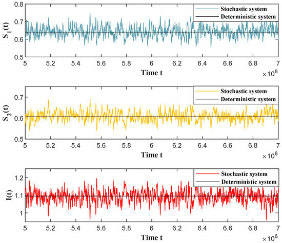
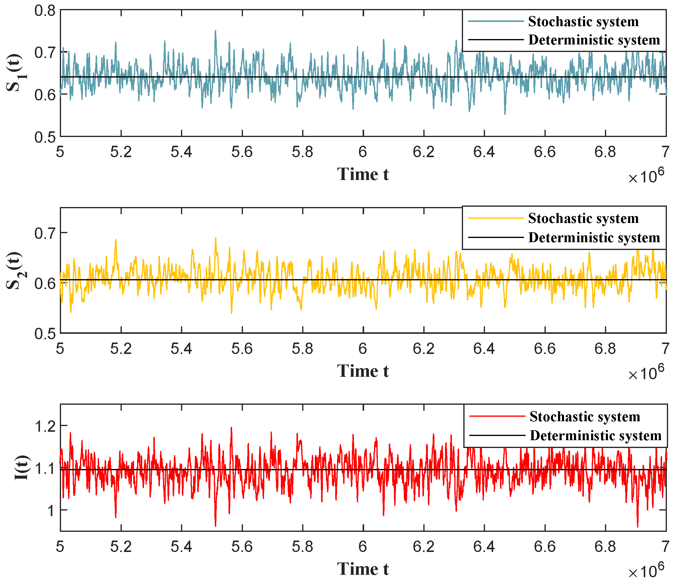
Through the trajectory images of $S_1\left(t\right),S_2\left(t\right),I\left(t\right)$ shown in Figure 1, we can easily observe that the disease will persist for a long time near the point ${\tilde{E}}^{\ast }={(0.6409,0.6062,1.0956,0,0)}^T$.

Figure 1. Solutions of $\{S_1\left(t\right),S_2\left(t\right),I\left(t\right)\}$ in a 3D deterministic model (11) and stochastic model (49) with an OU process.

We can obtain the variables $R_0=1.8833>1,R_0^s=1.80854>1$. Meanwhile, $\Sigma$ is computed by

$$\Sigma ={\Sigma }_1+{\Sigma }_2={\xi }_1^2{\left(\overline{M}\overline{J}\right)}^{-1}\overline{\Sigma }{\left({\left(\overline{M}\overline{J}\right)}^T\right)}^{-1}+{\xi }_2^2{\left(\tilde{M}\tilde{J}\right)}^{-1}\tilde{\Sigma }{\left({\left(\tilde{M}\tilde{J}\right)}^T\right)}^{-1}.$$

Substituting each parameter, the exact value of the matrix $\Sigma$ can be obtained as

$$\Sigma =\left(\begin{array}{ccccc}0.0008& 0.0004& -0.0008& -0.0018& -0.0003\\ 0.0004& 0.0005& -0.0006& -0.0004& -0.0011\\ -0.0008& -0.0006& 0.0010& 0.0017& 0.0011\\ -0.0018& -0.0004& 0.0017& 0.0083& 0\\ -0.0003& -0.0011& 0.0011& 0& 0.0045\end{array}\right).$$

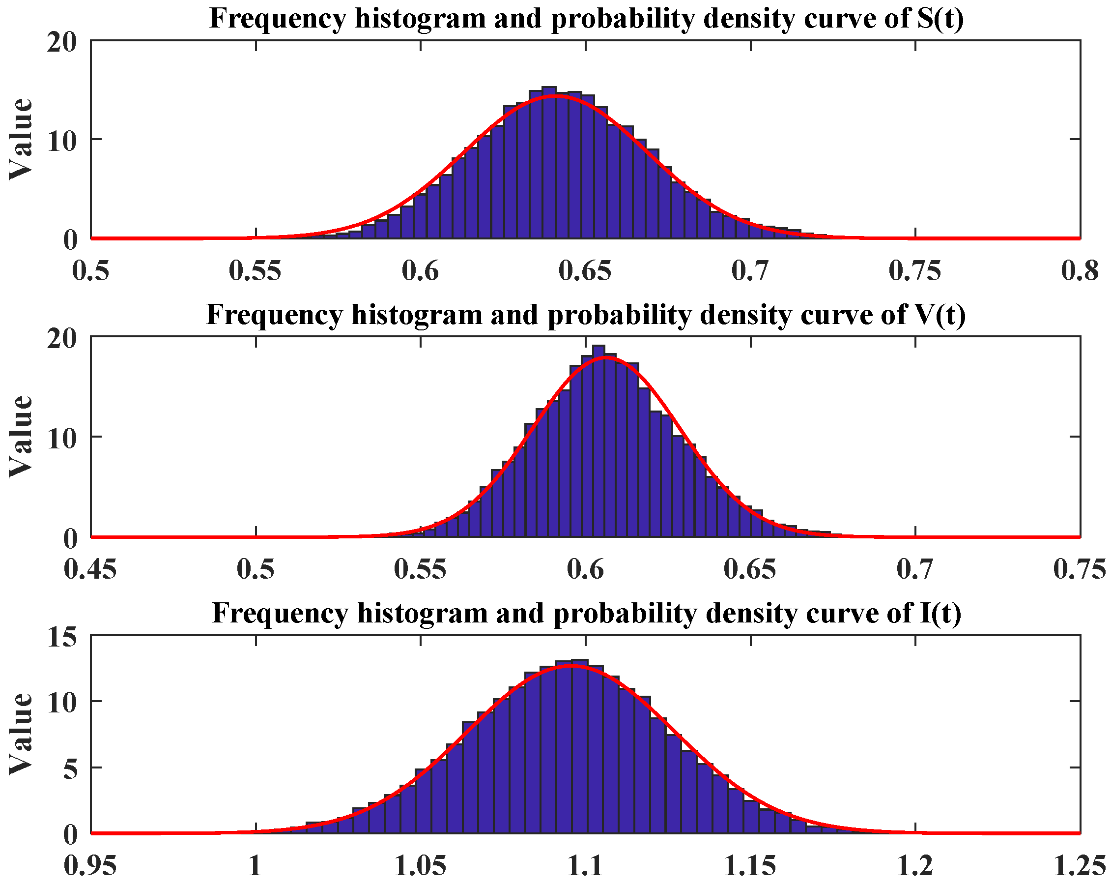
Around the quasi steady-state equilibrium point ${\tilde{E}}^{\ast }={(0.6409,0.6062,1.0956,0,0)}^T$, the solutions $Y\left(t\right)=(S_1\left(t\right),S_2\left(t\right),I\left(t\right),X_1\left(t\right),X_2\left(t\right))$ of system (11) follow the unique normal density function is as follows:

$$\Phi \left(Y\right)={\left(2\pi \right)}^{-{\displaystyle \frac{5}{2}}}{|\Sigma |}^{-{\displaystyle \frac{1}{2}}}{e}^{-{\displaystyle \frac{1}{2}}(S_1-0.6409,S_2-0.6062,I-1.0956,X_1,X_2){\Sigma }^{-1}{(S_1-0.6409,S_2-0.6062,I-1.0956,X_1,X_2)}^T}.$$

The solutions $(S_1\left(t\right),S_2\left(t\right),I\left(t\right),X_1\left(t\right),X_2\left(t\right))$ approximately follow a normal marginal density function is shown in Figure 2. And through probability theory and mathematical statistics theory, it can be concluded that the marginal density function is as follows:

$${\Phi }_1\left(S_1\right)={\displaystyle \frac{1}{\sqrt{2\pi }{\varphi }_1}}{e}^{-{\displaystyle \frac{{(S_1-S_1^{\ast })}^2}{2{\varphi }_1^2}}}=14.1047e^{-625{(S_1-0.6409)}^2},$$

$${\Phi }_2\left(S_2\right)={\displaystyle \frac{1}{\sqrt{2\pi }{\varphi }_2}}{e}^{-{\displaystyle \frac{{(S_2-S_2^{\ast })}^2}{2{\varphi }_2^2}}}=17.8412e^{-1000{(S_2-0.6062)}^2},$$

$${\Phi }_3\left(I\right)={\displaystyle \frac{1}{\sqrt{2\pi }{\varphi }_3}}{e}^{-{\displaystyle \frac{{(I-I^{\ast })}^2}{2{\varphi }_3^2}}}=12.6157e^{-500{(I-1.0956)}^2},$$

$${\Phi }_4\left(X_1\right)={\displaystyle \frac{1}{\sqrt{2\pi }{\varphi }_4}}{e}^{-{\displaystyle \frac{X_1^2}{2{\varphi }_4^2}}}=4.3790e^{-60.2410X_1^2},$$

$${\Phi }_5\left(X_2\right)={\displaystyle \frac{1}{\sqrt{2\pi }{\varphi }_5}}{e}^{-{\displaystyle \frac{X_2^2}{2{\varphi }_5^2}}}=5.9471e^{-111.1111X_2^2}.$$

Figure 2. The frequency histogram and marginal density function curve of $(S_1\left(0\right)=0.6409,S_2\left(0\right)=0.6062,I\left(0\right)=1.0956)$.

8. Conclusions and Discussions

This paper investigates a high-dimensional stochastic SIS epidemic model, represented by the stochastic system (3), in which the effective rate ${\lambda }_i$ is perturbed by the mean-reverting stochastic process. For the deterministic system, we establish the local asymptotic stability of both the disease-free equilibrium and the endemic equilibrium. In the corresponding stochastic model, we determine the stationary distribution by deriving a density function through the solution of the associated Fokker–Planck equation. Notably, the methodologies employed can be extended to other intriguing topics, including the computation of probability density functions for various stochastic epidemic models. However, a more comprehensive and systematic theory is needed to ascertain precise conditions and density functions effectively.

References

- Rahman, K.; Mitkari, S.R.; Shaikh, S. A tuberculosis model: Validating to study transmission dynamics with vaccination and treatment. Aligarh Bull. Math. 2020, 39, 35–45. [Google Scholar]
- Zhou, B.; Zhang, X.; Jiang, D. Dynamics and density function analysis of a stochastic SVI epidemic model with half saturated incidence rate. Chaos Soliton Fract. 2020, 137, 109865. [Google Scholar] [CrossRef]
- Wang, L.; Jiang, D. Ergodicity and threshold behaviors of a predator-prey model in stochastic chemostat driven by regime switching. Math. Methods Appl. Sci. 2021, 44, 325–344. [Google Scholar] [CrossRef]
- Huang, G.; Ma, W.; Takeuchi, Y. Global analysis for delay virus dynamics model with Beddington-DeAngelis functional response. Appl. Math. Lett. 2011, 24, 1199–1203. [Google Scholar] [CrossRef]
- Liu, Q. Stationary distribution and probability density for a stochastic SISP respiratory disease model with Ornstein-Uhlenbeck process. Commun. Nonlinear Sci. Numer. Simul. 2023, 119, 107128. [Google Scholar] [CrossRef]
- Zhang, H.; Sun, J.G.; Yu, P.; Jiang, D. Dynamical Behaviors of Stochastic SIS Epidemic Model with Ornstein-Uhlenbeck Process. Axioms 2024, 13, 353. [Google Scholar] [CrossRef]
- Han, B.; Zhou, B.; Jiang, D.; Hayat, T.; Alsaedi, A. Stationary solution, extinction and density function for a high-dimensional stochastic SEI epidemic model with general distributed delay. Appl. Math. Comput. 2021, 405, 126236. [Google Scholar] [CrossRef]
- Sun, J.G.; Gao, M.; Jiang, D. Threshold Dynamics and the Density Function of the Stochastic Coronavirus Epidemic Model. Fractal Fract. 2022, 6, 245. [Google Scholar] [CrossRef]
- Hyman, J.; Li, J. An intuitive formulation for the reproductive number for the spread of diseases in heterogeneous populations. Math. Biosci. 2000, 167, 65–86. [Google Scholar] [CrossRef] [PubMed]
- Anderson, R.M.; May, R.M.; Medley, G.F.; Johnson, A. A Preliminary Study of the Transmission Dynamics of the Human Immunodeficiency Virus (HIV), the Causative Agent of AIDS. Math. Med. Biol. 1986, 3, 229–263. [Google Scholar]
- Finch, S. Ornstein-Uhlenbeck Process. Stoch. Diff. Eq. 2004, 25, 61. [Google Scholar]
- Trostab, D.C.; Overman, E.A., II; Ostroff, J.H.; Xiong, W.; March, P. A model for liver homeostasis using modified mean-reverting Ornstein-Uhlenbeck process. Comput. Math. Methods Med. 2010, 11, 27–47. [Google Scholar] [CrossRef]
- Liu, Q. Dynamical analysis of a stochastic maize streak virus epidemic model with logarithmic Ornstein-Uhlenbeck process. J. Math. Biol. 2024, 89, 30. [Google Scholar] [CrossRef] [PubMed]
- Gao, M.; Jiang, D.; Ding, J. Dynamics of a chemostat model with Ornstein-Uhlenbeck process and general response function. Chaos Solitons Fractals 2024, 184, 114950. [Google Scholar] [CrossRef]
- Mao, X. Stochastic Differential Equations and Applications; Horwood: Chichester, UK; New York, NY, USA, 1997. [Google Scholar]
- Wu, F.; Mao, X.; Chen, K. A highly sensitive mean-reverting process in finance and the Euler-Maruyama approximations. J. Math. Anal. Appl. 2008, 348, 540–554. [Google Scholar] [CrossRef]
- Allen, E. Environmental variability and mean-reverting processes. Discret. Contin. Dyn.-Syst.-Ser. 2016, 21, 2073–2089. [Google Scholar] [CrossRef]
- Dixit, A.K.; Pindyck, R.S. Investment Under Uncertainty; Princeton University Press: Princeton, NJ, USA, 1994. [Google Scholar]
- Yang, Q.; Zhang, X.; Jiang, D. Dynamical Behaviors of a Stochastic Food Chain System with Ornstein-Uhlenbeck Process. J. Nonlinear Sci. 2022, 32, 34. [Google Scholar] [CrossRef]
- Ayoubi, T.B.H. Persistence and extinction in stochastic delay Logistic equation by incorporating Ornstein-Uhlenbeck process. Appl. Math. Comput. 2020, 386, 125465. [Google Scholar] [CrossRef]
- Kunita, H. Itô’s stochastic calculus: Its surprising power for applications. Stoch. Process. Their Appl. 2010, 120, 622–652. [Google Scholar] [CrossRef]
- Khas’miniskii, R.Z. Stochastic Stability of Differential Equations; Horwood: Chichester, UK, 1997. [Google Scholar]
- Higham, D.J. An algorithmic introduction to numerical simulation of stochastic differential equations. SIAM Rev. 2001, 43, 525–546. [Google Scholar] [CrossRef]
Disclaimer/Publisher’s Note: The statements, opinions and data contained in all publications are solely those of the individual author(s) and contributor(s) and not of MDPI and/or the editor(s). MDPI and/or the editor(s) disclaim responsibility for any injury to people or property resulting from any ideas, methods, instructions or products referred to in the content. |
© 2024 by the authors. Licensee MDPI, Basel, Switzerland. This article is an open access article distributed under the terms and conditions of the Creative Commons Attribution (CC BY) license (https://creativecommons.org/licenses/by/4.0/).