Mitigating an Epidemic on a Geographic Network Using Vaccination

Abstract

We consider a mathematical model describing the propagation of an epidemic on a geographical network. The size of the outbreak is governed by the initial growth rate of the disease given by the maximal eigenvalue of the epidemic matrix formed by the susceptibles and the graph Laplacian representing the mobility. We use matrix perturbation theory to analyze the epidemic matrix and define a vaccination strategy, assuming vaccination reduces the susceptibles. When mobility and the local disease dynamics have similar time scales, it is most efficient to vaccinate the whole network because the disease grows uniformly. However, if only a few vertices can be vaccinated, then we show that it is most efficient to vaccinate along an eigenvector corresponding to the largest eigenvalue of the Laplacian. We illustrate these results by calculations on a seven-vertex graph and a realistic example of the French rail network. When mobility is slower than the local disease dynamics, the epidemic grows on the vertex with largest number of susceptibles. The epidemic growth rate is more reduced when vaccinating a larger degree vertex; it also depends on the neighboring vertices. This study and its conclusions provide guidelines for the planning of a vaccination campaign on a network at the onset of an epidemic.

1. Introduction

The previous COVID-19 pandemic confirmed that mobility between countries or within a country is crucial to transmit diseases. Such a set of cities or countries can be described as vertices of a graph where edges represent communication links between them. A first coarse-grained approach based on complex networks (see, for example, the book [1]) assumes each vertex can have two states: healthy or infected, and that a transition matrix gives the probability for a vertex to infect its neighbor. This model can describe, for example, the propagation of a computer virus or a rumor on the internet [2]. An important notion here is centrality, i.e., the number of links associated with each vertex; vertices with large degrees play an important role in the propagation. The advantage of such a model is that the network is considered as a whole and one can rapidly estimate how infected it is; the disease dynamics is, however, crudely represented.

To better describe the disease dynamics, one can assume that each vertex has a population of susceptible and infected individuals. A pioneering study was conducted by Brockmann and Helbling [3] to analyze the propagation of influenza via airline routes. The mobility was described by an origin–destination probability matrix. To introduce more details in the mobility, a number of authors use metapopulations. This consists, for each city i, of counting individuals who stay at i and others who travel to another city j; see, for example, the discussions by Keeling et al. [4] and Sattenspiel and Dietz [5]. Later, Colizza et al. [6] analyzed the model in detail and introduced the concepts of local and global epidemic thresholds. Poletto et al. [7] also examined how fluctuations of the mobility fluxes affect these thresholds. From another point of view, Gautreau et al. [8] used a similar model and statistical physics methods to predict the arrival of a disease in a country. Gao [9] studied a simpler model where populations are split into frequent and rare travelers; he analyzed a two patch system and found that, in general, diffusion reduces disease spread. See also the analysis of Cantin and Silva [10] and their results on a two patch network. All these models provide an accurate description of mobility; however, their analysis is complicated even for moderately sized networks and it is not easy to have a picture of the global state of the network. Also, it is not always possible to obtain and predict population movements. Finally, these models have many parameters and these are not easy to estimate from real data.

In a recent article, we considered an SIR model on each vertex, where the vertices are coupled by a graph Laplacian [11], a natural generalization of the SIR model to a network. Assuming a slow diffusion, we estimated the coefficient by examining the arrival times of the epidemic front in China, Vietnam, Iran, Italy, etc., and using this, predicted the arrival of the COVID-19 epidemic in Mexico [12]. We also analyzed how deconfining a large city connected to a smaller region can cause a secondary outburst in the smaller city.

The problem of vaccine allocation introduces another complication because the disease dynamics are, in general, nonlinear. There is a large body of literature on the strategies for vaccination, see, for example, [13]. Most studies focus on preventing deaths and hospitalizations. Vaccination can also be used to prevent geographical dissemination of the disease, there are however few articles on this topic. For example, Matrajt et al. [14] studied vaccine allocations at the onset of an epidemic. They coupled a mathematical model with a genetic algorithm to optimally distribute vaccines in a complete graph of Asian cities and found that it is best to distribute vaccines over the network and that an epidemic can be mitigated if vaccination occurs in the first few weeks. Optimal control can also be used to allocate vaccines, like in the article by Lemaitre et al. [15] who chose the total number of cases as an objective function to be minimized. For the different scenarios they consider, the authors also found that a global strategy at the network level is more effective.

We consider the problem of a number of vaccine doses to be distributed on the network at the onset of an epidemic and assume that vaccination prevents the dissemination of the disease. This is true for many vaccines; a very important example is smallpox, which has completely disappeared due to a massive vaccination campaign. Other diseases, like COVID-19, only partially reduce the transmissivity of the disease. The reduction in the susceptibles is small because a small proportion of the population is usually vaccinated. Matrajt introduced an epidemic prevention potential to measure the effect of vaccination. In a similar way, in our study [11] we defined the epidemic growth rate as the maximum eigenvalue $\lambda$ of the epidemic matrix M: the sum of the diagonal matrix $\mathrm{diag}(\beta S-\gamma )$ and the graph Laplacian mobility matrix. This is a generalization to our geographic model of the well-known $R_0$ criterion for the classical models of epidemiology. If $\lambda$ is large, the maximum number of infected will be large, and vice versa, so that $\lambda$ is a measure of the size of the outbreak.

Our preliminary results [11] indicated that it is more effective to vaccinate high degree vertices and not neighbors. Here, we conduct a more in depth study of the problem to confirm/disprove these findings. In particular, we ask the following questions: which vertex, if vaccinated, will reduce $\lambda$ the most? What is the role of the degree? Is it better to vaccinate two vertices or three vertices instead of one? What role do the eigenvectors of the graph Laplacian play?

To address these questions, we analyze the epidemic matrix M. To estimate the maximum eigenvalue of M, we use matrix perturbation theory [16] where the eigenvalues are written as a power series of a small parameter. The perturbation scheme reveals the interplay between the topology of the network and the dynamics of the infection. We study two different regimes, depending whether the disease propagates inside a country or between countries. In the first regime (FD), the diffusion is fast and dominates the disease dynamics. The corrections at orders one and two of the maximal eigenvalue show that it is most efficient to uniformly vaccinate the network. We then examine how $\lambda$ varies when vaccination is applied along an eigenvector $V^k$ of the Laplacian and found that it is minimum when k is large. We illustrate these findings on a seven-vertex graph and give special graphs (complete, stars) for which this argument does not hold. Finally, we study numerically a more realistic situation where the Laplacian has weights corresponding to routes more traveled than others and where the argument holds again.

A second interesting regime (SD) is when the diffusion is slow compared to the local disease dynamics. Then, the eigenvalues depend on the degree of each vertex at 1st order and on the neighbors for the 2nd order. We give an example on a seven-vertex graph. The results confirm that the perturbation approach gives an excellent approximation of $\lambda$.

The article is organized as follows, Section 2 presents the model and the perturbation method. The limit FD, when the disease dynamics and mobility have the same timescales is detailed in Section 3 and several graphs are analyzed numerically in Section 4. In Section 5, we describe the limit SD when the disease dynamics dominates the mobility and conclusions are presented in Section 6.

2. The Model and the Perturbation Method

We recall the model introduced in [11] describing the propagation of an epidemic on a geographical network where the vertices are indexed $1,2,\dots ,n$

$$\left\{\begin{array}{c}\dot{S}=\alpha LS-\beta SI,\hfill \\ \dot{I}=\alpha LI+\beta SI-\gamma I.\hfill \\ \dot{R}=\alpha LR+\gamma I.\hfill \end{array}\right.$$

(1)

where $S={(S_1,S_2,\dots ,S_n)}^T,I={(I_1,I_2,\dots ,I_n)}^T$ and $R={(R_1,R_2,\dots ,R_n)}^T$ are, respectively, the vectors of the susceptibles, infected, and recovered, L is the graph Laplacian $n\times n$ matrix [17], $\beta , \gamma$ are, respectively, the infection and recovery ratios, and where we denote the vector ${(S_1{I}_1,S_2{I}_2,\dots ,S_n{I}_n)}^T$ by $SI$. The quantities $S, I$ and R can be considered as numbers or proportions. For simplicity, we assume that the total population at each vertex is the same.

We have the following definition:

Definition 1. 

The graph Laplacian matrix L is a real symmetric negative semi-definite matrix, such that

• $L_{kl}=L_{lk}\ne 0$ if k and l are connected, 0 otherwise,
• $L_{kk}=-{\sum }_{l\ne k}{L}_{kl}$ .

We want to understand how the network topology affects the propagation of the epidemic. Therefore, we assume, in most of the paper, that the non zero $L_{lk}$’s are equal to one.

The model (1) is a simplified origin–destination mobility model (like [3]) coupled to an SIR epidemic model, since we assumed symmetry in the transition matrix. The diffusion through the Laplacian graph is a first-order approximation of dispersion of all the subjects (susceptibles, infected, and recovered) similar to Fourier’s or Ohm’s law. For example, Murray [18] uses such a model in continuum space to describe the propagation of rabies.

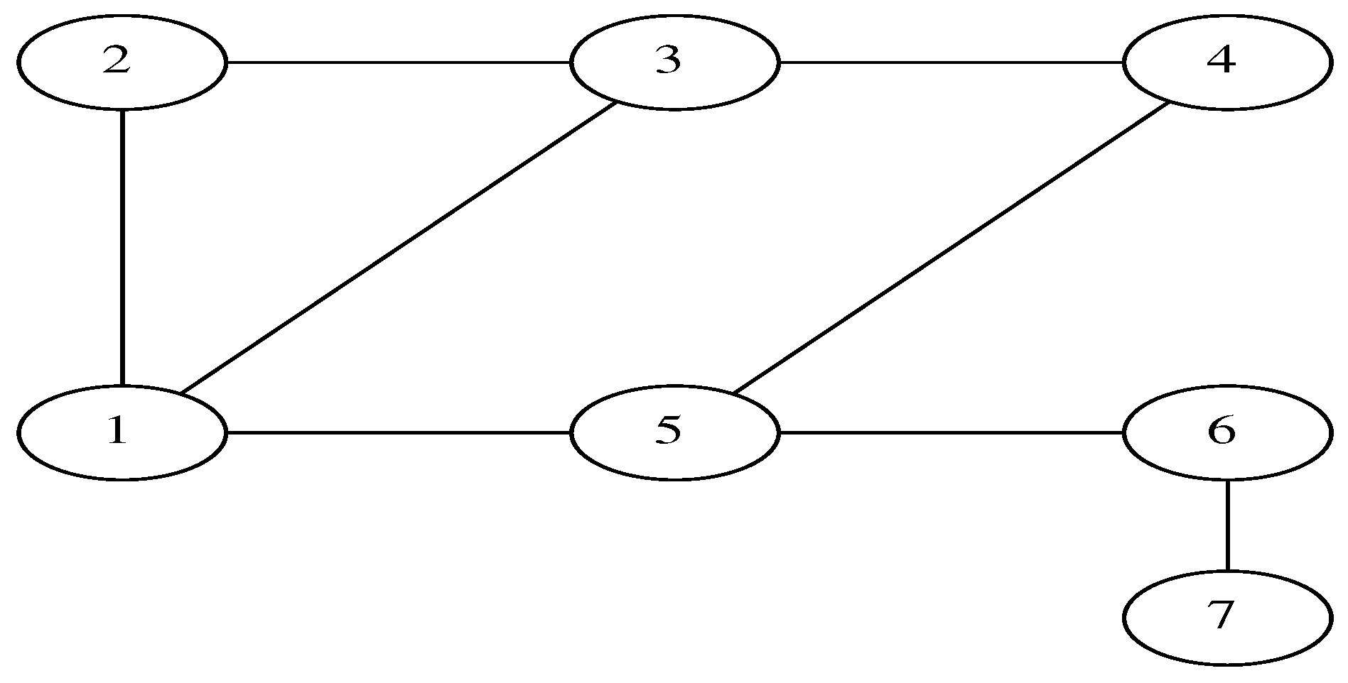
To illustrate the model, consider the seven-vertex graph shown in Figure 1. The weightless graph Laplacian matrix is

$$L=\left(\begin{array}{ccccccc}-3& 1& 1& 0& 1& 0& 0\\ 1& -2& 1& 0& 0& 0& 0\\ 1& 1& -3& 1& 0& 0& 0\\ 0& 0& 1& -2& 1& 0& 0\\ 1& 0& 0& 1& -3& 1& 0\\ 0& 0& 0& 0& 1& -2& 1\\ 0& 0& 0& 0& 0& 1& -1\end{array}\right)$$

The graph Laplacian matrix has important properties, see Ref. [17]; in particular, it is a finite difference approximation of the continuous Laplacian [19]. The eigenvalues of L are the n non-positive real numbers ordered and denoted as follows:

$$0=-{\omega }_1^2\ge -{\omega }_2^2\ge \dots \ge -{\omega }_n^2.$$

The eigenvectors $\{V^1,\dots ,V^n\}$ satisfy

$$L{V}^j=-{\omega }_j^2{V}^j.$$

and can be chosen to be orthonormal with respect to the standard scalar product in ${\mathbb{R}}^n$, i.e., $(V^i,V^j)={\delta }_{i,j}$ where ${\delta }_{i,j}$ is the Kronecker symbol. The eigenvector $V^1$ corresponding to $\omega =0$ has equal components. In the following, we will use the vector

$$\mathbf{1}={(1,\dots ,1)}^T=\sqrt{n}{V}^1.$$

In connection with problem (1), we introduce the following matrix:

Definition 2. 

For a graph with Laplacian L and initial proportion of susceptibles S, the epidemic matrix M is

$$M=\alpha L+\beta \mathrm{diag}\left(S\right)-\gamma \mathrm{Id},$$

(2)

where $\mathrm{Id}$ is the identity matrix of order n.

For short time, we can assume that S is constant so that Equation (1) imply

$$\dot{I}=MI.$$

Note that I varies exponentially. The matrix M is symmetric. Its eigenvalues are real because the eigenvalues of L are real and the additional terms will shift them onto the real axis. The maximum eigenvalue $\lambda$ of M gives the initial rate of growth of the infected on the network. We define the epidemic rate in the following way.

Definition 3. 

The epidemic growth rate is the maximum eigenvalue λ of M.

Note that when the network is reduced to one vertex $n=1$, the Laplacian matrix is the scalar 0 so that we recover the standard SIR epidemic criterion. For our geographic model, the situation is more complicated and the maximal eigenvalue $\lambda$ controls the growth of I. Our main goal in this article is to discover the vaccination policy that minimizes $\lambda$. For that we use eigenvalue perturbation theory.

We will consider two limiting cases of mobility described by the diffusion operator L:

Definition 4. 

If $\alpha , \beta$ and γ are of the same order, we will term the regime “fast diffusion” (FD). If $\alpha \ll \beta$ and $\alpha \ll \gamma$ the regime will be called “slow diffusion” (SD).

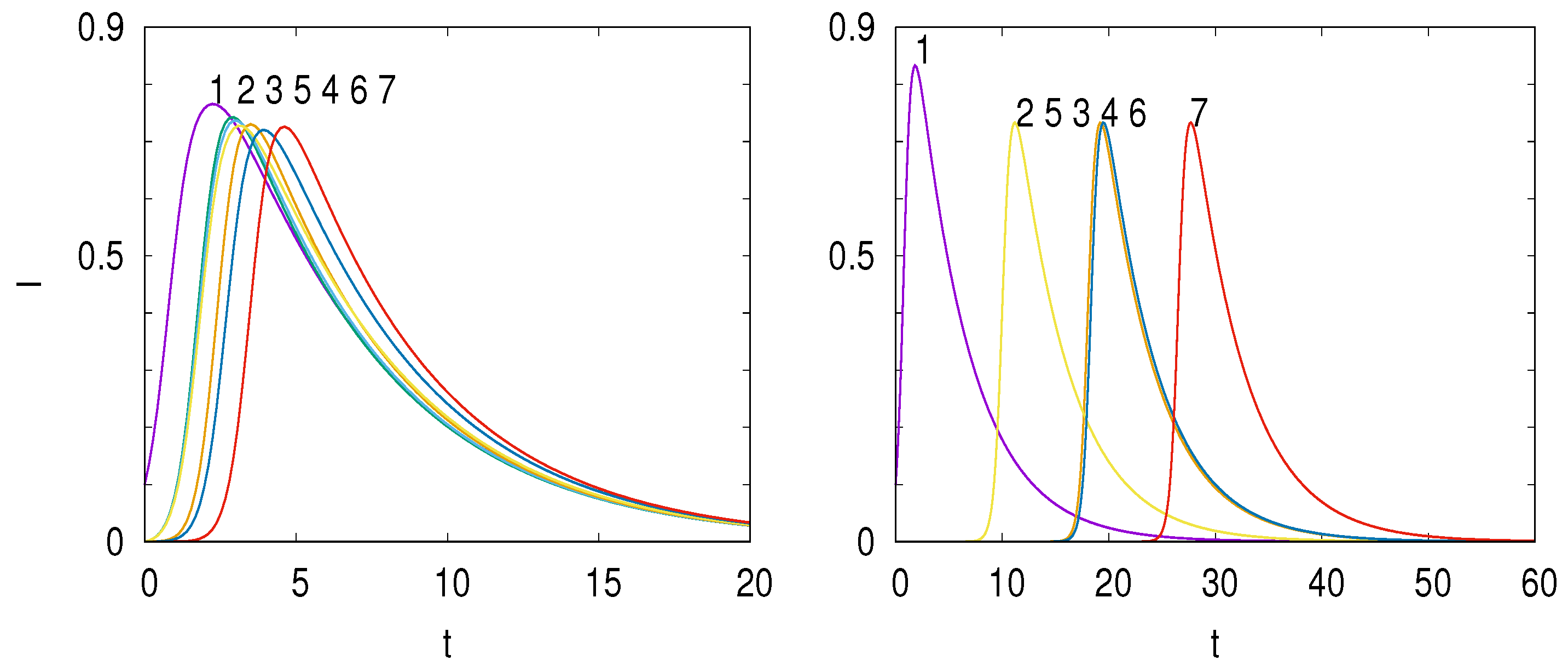
To illustrate these two regimes, Figure 2 shows the time evolution of the infected $I_k\left(t\right),k=1,\dots ,7$ for the network shown in Figure 1 for a fast diffusion (left panel) and a slow diffusion (right panel).

We can make the following remarks:

• FD occurs in a highly connected city or small country. The parameter $\alpha$ is significant compared to $\beta$ and $\gamma$. Then, the infected will grow uniformly across the network. One can then study how a small variation $ϵs$ of the susceptibles S due to the initial vaccination affects the epidemic growth rate. The order 0 eigenvalues are

  $$0=-{\omega }_1^2\ge -{\omega }_2^2\ge \dots \ge -{\omega }_n^2.$$

  and the order 0 eigenvectors are the eigenvectors of the Laplacian graph L, $\{V^1,\dots ,V^n\}$.
• SD corresponds to a slow diffusion so $\alpha$ is small. An example is the small coupling between vertices like for air travel between different countries. We used it to describe the propagation of COVID-19 between the main world airports in the spring 2020 [11]. Here, as shown in Figure 2, we see a succession of well separated peaks as the outbreak starts and falls on the different vertices. We consider here that the perturbation is the Laplacian graph parameterized by $\alpha$. The order 0 eigenvalues are $\mathrm{diag}\left(\beta S\right)-\gamma \mathrm{Id}$ and the order 0 eigenvectors are the ones of the canonical base.

Perturbation Theory

The matrix M can be written as

$$M=M_0+ϵR,$$

(3)

where $M_0, R$ depend on the assumptions, FD or SD, that we make.

The principle of this perturbation theory for eigenvalues and eigenvectors of a matrix [16] is to write the expansions of an eigenvalue $\lambda$ of M and its corresponding eigenvector v as

$$\begin{array}{c}\hfill \lambda ={\lambda }^0+ϵ{\lambda }^1+{ϵ}^2{\lambda }^2+{ϵ}^3{\lambda }^3+\dots ,\end{array}$$

(4)

$$\begin{array}{c}\hfill v=v_0+ϵv_1+{ϵ}^2{v}_2+{ϵ}^3{v}_3+\dots \end{array}$$

(5)

and write the different orders in $ϵ$. For small enough $ϵ$, this expansion can be shown to converge [16].

We introduce the expansions above in the eigenvalue equation $Mv=\lambda v,$ and the first three orders in $ϵ$ yield

$$\begin{array}{c}\hfill (M_0-{\lambda }^0)v_0=0,\end{array}$$

(6)

$$\begin{array}{c}\hfill (M_0-{\lambda }^0)v_1=({\lambda }^1-R)v_0,\end{array}$$

(7)

$$\begin{array}{c}\hfill (M_0-{\lambda }^0)v_2={\lambda }^2{v}_0+{\lambda }^1{v}_1-R{v}_1.\end{array}$$

(8)

These linear equations have solutions if their right-hand side is orthogonal to the kernel of ${(M_0-{\lambda }^0)}^{†}=(M_0-{\lambda }^0)$. This is the solvability condition. From the solvability conditions, we obtain ${\lambda }^1$ and ${\lambda }^2$ as

$${\lambda }^1={\displaystyle \frac{(v_0,R{v}_0)}{(v_0,v_0)}},$$

(9)

$${\lambda }^2={\displaystyle \frac{(v_0,R{v}_1-{\lambda }^1{v}_1)}{(v_0,v_0)}}.$$

(10)

The order 1 eigenvector $v_1$ solves Equation (7).

In both cases, FD and SD, the matrix M is symmetric so that its eigenvalues are real. Then, for small $ϵ$, the order of the eigenvalues will not vary and the maximum eigenvalue $\lambda$ will reduce to the maximum eigenvalue of $M_0$.

The eigenvalues of M are roots of a polynomial whose coefficients depend on $ϵ$; therefore, they depend analytically on $ϵ$. This means that the expansion converges and generically there are no singularities [16].

3. FD Fast Diffusion: Perturbation Results

In the FD framework, we assume that $\alpha$ is comparable to $\beta , \gamma$. To reduce the dispersion of the disease, the vaccination decreases the proportion of susceptibles. The number of susceptibles can be chosen as equal to 1 in the absence of perturbation. We assume the change in S to be small, $O\left(ϵ\right)$ so that at a vertex i $S_i$ is given by

$$S_i=1-ϵs_i,$$

(11)

then $-ϵs_i$ is the reduction in the number of susceptibles at vertex i due to vaccination.

The matrix M can be written as

$$M=M_0+ϵR,M_0=L+(\beta -\gamma )\mathrm{Id},R=-\beta \left(\begin{array}{cccc}{s}_1& 0& \dots & 0\\ 0& s_2& \ddots & ⋮\\ ⋮& \ddots & \ddots & 0\\ 0& \dots & 0& s_n\end{array}\right)$$

(12)

The maximum eigenvalue $\lambda$ of M corresponds to the 0 eigenvalue of the Laplacian. Then, we have

$${\lambda }^0=\beta -\gamma .$$

(13)

In our special case $(M_0-{\lambda }^{0}Id)=L$, so the Equations (6)–(8) above reduce to

$$\begin{array}{c}\hfill L{v}_0=0,\end{array}$$

(14)

$$\begin{array}{c}\hfill L{v}_1=({\lambda }^1-R)v_0,\end{array}$$

(15)

$$\begin{array}{c}\hfill L{v}_2={\lambda }^2{v}_0+({\lambda }^1-R)v_1.\end{array}$$

(16)

The Laplacian has real eigenvalues and orthogonal eigenvectors

$$L{V}^i=-{\omega }_i^2{V}^i,$$

(17)

where ${\omega }_1=0$ and $V^1$ is the constant vector. The other eigenvalues verify

$$-{\omega }_n^2\le \cdots \le -{\omega }_1^2=0.$$

(18)

We assume the graph to be simply connected so that there is only one eigenvalue zero [17]. The matrix L is therefore singular and special care must be taken when solving the system. The standard way to solve the system is to use the singular value decomposition of L. Since L is symmetric, this reduces to projecting the solution and the right-hand side on the eigenvectors of L. Therefore, $v_0=V^1$ where $V^1$ is the constant normalized eigenvector. The Formulas (9) and (10) become

$${\lambda }^1=(V^1,R{V}^1),$$

(19)

$${\lambda }^2=\left(V^1,(R-{\lambda }^1)v_1\right),$$

(20)

where $v_1$ solves the linear Equation (15).

Our main goal is to define possible vaccination policies and reveal an optimal one, in the sense that

$$\lambda ={\lambda }^0+ϵ{\lambda }^1+{ϵ}^2{\lambda }^2+O\left({ϵ}^3\right)$$

is minimum. Equation (2) shows that the network determines $\lambda$. Following this observation the following questions arise: is it better to uniformly vaccinate the network? Or if this is not possible, what are the best vertices to vaccinate?

In view of these questions, three vaccination strategies are possible

(i)

Reduce the proportion of susceptibles of $S_i$ uniformly on all vertices, then $s_i\ge 0,i=1,\dots ,n$.

(ii)

Adjust $S_i$ globally using an eigenvector $V^k$ of the Laplacian L, i.e., $S=\mathbf{1}-ϵV^k$. Then, $s_i$ can be positive or negative.

(iii)

Reduce $S_i$ on some vertices and not others, then $s_i>0,$ for some $i=1,\dots ,n$.

• Approach (i) is to vaccinate uniformly all vertices. This assumes that we have the logistics to distribute the vaccine throughout the network. It is the simplest of strategies and will be the benchmark to test the other strategies. Approach (ii) is not practical since we cannot increase $s_i$, we can only decrease it. Despite this, we consider it in this theoretical section. Approach (iii) assumes there are a limited number of vertices that can be vaccinated. Then, we need to choose which ones.

We can state the following

• Mathematical program
• Minimize the epidemic growth rate $\lambda$ such that ${\sum }_{i=1}^n{s}_i$ is constant.
• For strategies (i) and (iii) $s_i\ge 0$.
• For strategy (ii) there are no positivity constraints on $s_i$.

3.1. The First Order ${\lambda }^1$

First, consider the simple situation where all vertices are vaccinated with the same amount, $s_1=s_2=,\dots ,=s_n=s$. Then

$$M=L+(\beta -\gamma )\mathrm{Id}-\beta ϵs\mathrm{Id}=L+\left[\beta \right(1-ϵs)-\gamma ]\mathrm{Id}.$$

Then, the maximum eigenvalue of M is

$$\lambda =\beta (1-ϵs)-\gamma .$$

(21)

This result is exact.

When the $s_i$ are different, we have the following result.

Theorem 1. 

Let G be a connected graph with n vertices and assume that the number of susceptibles at each vertex i is $S_i=1-ϵs_i$. Then the epidemic growth rate is

$$\lambda =\beta -\gamma -ϵ{\displaystyle \frac{\beta }{n}}\sum _{i=1}^n{s}_i+O\left({ϵ}^2\right).$$

(22)

Proof. 

This is a direct consequence of Equation (19) because $v_0=V^1$ the constant eigenvector. □

We can make the following remarks:

(i)

When all vertices are vaccinated, we recover the result (21) and the $O\left({ϵ}^2\right)$ term is zero.

(ii)

If only one vertex is vaccinated, then

$$\lambda =\beta -\gamma -ϵ{\displaystyle \frac{\beta }{n}}+O\left({ϵ}^2\right).$$

(23)

This expression does not depend on the vertex that is vaccinated.

(iii)

Note that ${\lambda }^1$ is always negative.

(iv)

From Theorem 1, ${\lambda }^1$ is minimal when ${\sum }_{i=1}^n{s}_i$ is maximal. In other words, we can minimize ${\lambda }^1$ and thus the epidemic growth rate $\lambda$ by increasing the total percentage of the vaccinated population on the network regardless of their location.

3.2. Spectral Approach

Using the eigenvectors of the Laplacian matrix L (17) one can calculate ${\lambda }^2$ in closed form. We have

Theorem 2. 

Let G be a connected graph with n vertices and assume that the susceptibles at each vertex i are $S_i=1-ϵs_i$. Then the epidemic growth rate is

$$\lambda =\beta -\gamma -ϵ{\displaystyle \frac{\beta }{\sqrt{n}}}(s,V^1)+{ϵ}^2{\displaystyle \frac{\beta }{n}}\sum _{k=2}^n{\displaystyle \frac{1}{{\omega }_k^2}}{(s,V^k)}^2+O\left({ϵ}^3\right),$$

(24)

where $s={(s_1,s_2,\dots ,s_n)}^T$ and $(V^1,V^2,\dots ,V^n)$ are the eigenvectors of the graph Laplacian L corresponding to the eigenvalues $0=-{\omega }_1^2>-{\omega }_2^2\ge \cdots \ge -{\omega }_n^2$.

Proof. 

We have

$${\lambda }^2=(V^1,(R-{\lambda }^1)v_1),$$

where

$$L{v}_1=({\lambda }^1-R)V^1.$$

We expand $v_1$ on the basis of the eigenvectors of L

$$v_1=\sum _{k=1}^n{\alpha }_k{V}^k,$$

plug it into the equation above, and then project it onto each eigenvector $V^k$ to yield ${\alpha }_k$. We obtain ${\alpha }_1=0$ as a solvability condition and

$$v_1=\sum _{k=2}^n{\displaystyle \frac{1}{{\omega }_k^2}}(R{V}^1,V^k)V^k,$$

(25)

where

$$R{V}^1=-{\displaystyle \frac{\beta }{\sqrt{n}}}{(s_1,s_2,\dots ,s_n)}^T$$

We can now compute ${\lambda }^2$, as

$${\lambda }^2=(V^1,(R-{\lambda }^1)v_1)=\sum _{k=2}^n{\displaystyle \frac{1}{{\omega }_k^2}}(R{V}^1,V^k)(V^1,(R-{\lambda }^1)V^k)$$

We have

$$(V^1,(R-{\lambda }^1)V^k)=(V^1,R{V}^k)$$

because $V^1$ and $V^k$ are orthogonal. We finally obtain

$${\lambda }^2=\sum _{k=2}^n{\displaystyle \frac{1}{{\omega }_k^2}}{(R{V}^1,V^k)}^2={\displaystyle \frac{\beta }{n}}\sum _{k=2}^n{\displaystyle \frac{1}{{\omega }_k^2}}{(s,V^k)}^2.$$

□

Note that the correction ${\lambda }^2$ is always positive.

An important theorem follows from the estimate (24).

Theorem 3. 

Let G be a connected graph with n vertices and assume that the vector of susceptibles is $S=\mathbf{1}-ϵ\sqrt{n}{V}^k$, where $V^k$ is the kth eigenvector of the graph Laplacian L. Then the epidemic growth rate is

$$\lambda =\beta -\gamma +{ϵ}^2{\displaystyle \frac{\beta }{{\omega }_k^2}}+O\left({ϵ}^3\right).$$

(26)

The eigenvalue λ is minimum when $k=n$.

Proof. 

Choosing ${(s_1,s_2,\dots ,s_n)}^T=\sqrt{n}{V}^k$ where $V^k, k\ge 2$ is an eigenvector of L leads to ${\lambda }^1=0$.

In Equation (19), we have from the orthogonality of $V^k,k>1$ to $V^1$

$$\sum _{i=1}^n{s}_i=\sum _{i=1}^n{V}_i^k=0.$$

Assume $S=\sqrt{n}(V^1-ϵV^k)$. Then

$${\lambda }^2=\beta {\displaystyle \frac{1}{{\omega }_k^2}}.$$

From the order relation (18), this quantity decreases monotonically as k varies from 2 to n.

□

In other words, if we choose ${(s_1,s_2,\dots ,s_n)}^T=\sqrt{n}{V}^k$, the correction ${\lambda }^2$ decreases as k increases.

3.3. Comparing the Different Vaccination Strategies

From this analysis, we can discuss how different vaccination policies proposed in the beginning of Section 3 affect $\lambda$.

(i)

Uniform vaccination on the network, i.e., $S=(1-ϵ{\displaystyle \frac{1}{n}})\mathbf{1}$ and $s_i=1/n, i=1,2,\dots ,n$. Then

$$\lambda =\beta (1-ϵ{\displaystyle \frac{1}{n}})-\gamma .$$

(27)

This is the optimal vaccination strategy for the network because there is no positive term $O\left({ϵ}^2\right)$.

(ii)

Vaccination following the eigenvector $V^k$, then $S=\mathbf{1}-ϵ\sqrt{n}{V}^k$. We then have

$${\lambda }^0=\beta -\gamma ,{\lambda }^1=0,{\lambda }^2={\displaystyle \frac{\beta }{{\omega }_k^2}}$$

so that

$$\lambda =\beta -\gamma +{ϵ}^2{\displaystyle \frac{\beta }{{\omega }_k^2}}+O\left({ϵ}^3\right).$$

(28)

This expression is minimum for $k=n$. As indicated above, vaccinating along an eigenvector $V^k$ is not realistic because $V_j^k$ can be positive or negative and $S_j$ cannot increase at certain vertices j.

(iii)

Vaccination of $j<n$ vertices of the network, i.e., $S_k=1-{\displaystyle \frac{1}{j}},k=1,\dots ,j,S_k=1,k=j+1,\dots ,n$.

This is the most difficult situation because we cannot control ${\lambda }^2$. We have

$${\lambda }^0=\beta -\gamma ,{\lambda }^1=-{\displaystyle \frac{\beta j}{n}}$$

so that

$$\lambda =\beta -\gamma -ϵ{\displaystyle \frac{\beta }{n}}+O({ϵ}^2)=\beta (1-ϵ{\displaystyle \frac{1}{n}})-\gamma +O\left({ϵ}^2\right).$$

(29)

We recover the same expression at 1st order as in (i). However, the term $O\left({ϵ}^2\right)$ will vary. Only when $j=n$, $O\left({ϵ}^2\right)=0$ because ${\lambda }^i=0,i\ge 2$.

From the results of (ii) and (iii), a strategy emerges: one can vaccinate some vertices j so that the s vector becomes close to an eigenvector $V^k$, preferably of high order. We will see below that this method gives a $\lambda$ that is minimal so that this strategy is optimal for $j<n$.

4. FD: Two Examples

Here, we examine numerically the matrix M and its maximal eigenvalue $\lambda$ for different graphs to emphasize the role of the graph topology.

4.1. The Seven-Vertex Graph

For the seven-vertex graph considered above, we computed the largest eigenvalue of the matrix M with $S=\mathbf{1}+0.3\sqrt{7}{V}^k$ for $k=2,\dots n$. We chose $ϵ=0.3$ as a small quantity and $\beta =\gamma =1$ for simplicity. The results are presented in the table below.

The last column of

Table 1. Maximum eigenvalue $\lambda$ of M for $S=\mathbf{1}+0.3\sqrt{7}{V}^k$ (middle column) and perturbation estimate (right column).

k	$\mathit{\lambda }$	Perturbation ${\mathit{\lambda }}_{\mathit{per}}$ (28)	Relative Error
2	$1.204{10}^{-1}$	$2.314{10}^{-1}$	$4.8{10}^{-1}$
3	$6.073{10}^{-2}$	$5.958{10}^{-2}$	$1.9{10}^{-2}$
4	$4.173{10}^{-2}$	$4.086{10}^{-2}$	$2.1{10}^{-2}$
5	$2.716{10}^{-2}$	$2.791{10}^{-2}$	$2.7{10}^{-2}$
6	$2.547{10}^{-2}$	$2.405{10}^{-2}$	$5.9{10}^{-2}$
7	$1.821{10}^{-2}$	$1.825{10}^{-2}$	$2.3{10}^{-3}$

is the relative error

$$|\lambda -{\lambda }_{per}|/\lambda ,$$

where ${\lambda }_{per}$ is given by (28). Note how $\lambda$ decreases between $2\le k\le 7$. The optimal vaccination policy is the one that follows $V^7$. The eigenvalue $\lambda$ varies from 0.12 to 0.018 as s follows $V^2$ or $V^7$. The perturbation estimate is shown in the third column and the relative error in the fourth. It is about ${ϵ}^2$ except for $k=2$. The eigenvector $V^2$ has large components on vertices 6 and 7 and smaller components on the other vertices. Then, the perturbation approach becomes less accurate.

The eigenvectors of the Laplacian are plotted in Figure 3. As expected, the low-order eigenvectors $V^2,V^3,V^4$ vary on scales comparable to the size of the graph while the high-order eigenvectors $V^5,V^6,V^7$ oscillate on smaller scales.

It is difficult to relate the results of Table 1 to the practical situation of vaccinating individual vertices. To study this, we now vaccinate two or three vertices and compute the epidemic growth rate. The sum of the S vector is the same for both situations, and corresponds to a limited amount of vaccines being distributed over a geographic region. We chose the parameters $ϵ=1,\beta =1.12,\gamma =1$ so that the eigenvalues $\lambda$ are distributed on both sides of zero. As discussed above, the minimum of $\lambda$ corresponds to a uniform vaccination of the network, it is

$${\lambda }_{\min }=\beta (1-ϵ{\displaystyle \frac{1}{n}})-\gamma =-0.04.$$

(30)

This quantity will provide a benchmark to measure how efficient the vaccination is.

For two vaccinated vertices $i, j$, we choose $s_i=0.5,s_j=0.5$ so that $s_i+s_j=1$.

Table 2. Maximal eigenvalue $\lambda$ and argmax of the projection p (see (31)) when vaccinating two vertices $i, j$ for the seven-vertex graph of Figure 3. The parameters are $ϵ=1,\beta =1.12,\gamma =1$.

i	j	p	$\mathit{\lambda }$	i	j	p	$\mathit{\lambda }$	i	j	p	$\mathit{\lambda }$
3	6	6	$-2.1751{10}^{-2}$	2	5	6	$-9.5849{10}^{-3}$	2	4	6	$6.1549{10}^{-3}$
1	6	4	$-1.8658{10}^{-2}$	1	7	5	$-7.9345{10}^{-3}$	3	4	4	$7.1014{10}^{-3}$
2	6	5	$-1.6895{10}^{-2}$	1	4	7	$-7.8741{10}^{-4}$	1	3	6	$7.5348{10}^{-3}$
3	5	7	$-1.3008{10}^{-2}$	4	5	3	$-5.6481{10}^{-3}$	5	7	2	$8.0539{10}^{-3}$
1	5	5	$-1.1325{10}^{-2}$	2	7	3	$-4.7755{10}^{-3}$	1	2	3	$1.4141{10}^{-2}$
3	7	4	$-1.0303{10}^{-2}$	4	7	4	$1.6008{10}^{-4}$	2	3	2	$1.7100{10}^{-2}$
4	6	3	$-1.0146{10}^{-2}$	5	6	4	$2.1799{10}^{-4}$	6	7	2	$4.4036{10}^{-2}$

gives for $i, j$, the maximum of the projection on the eigenvectors

$$p={\mathrm{argmax}}_{1<k\le n}\left|(S,V^k)\right|,$$

(31)

and the epidemic growth rate $\lambda$.

As expected, the largest $\lambda$ corresponds to a p that is maximal on the low-order eigenvectors and vice versa. This is an average trend and there are some exceptions such as (1,3), (2,4). This is because the second-largest projection is on $V^2$, see Figure 3.

For three vaccinated vertices $i, j, k$, we choose $s_i=s_j=s_k=1/3$ so that $s_i+s_j+s_k=1$. We define the projection similarly to (31). The results are presented in

Table 3. Maximal eigenvalue $\lambda$ and projection p when vaccinating three vertices $i, j, k$ for the seven-vertex graph of Figure 3.

i	j	k	p	$\mathit{\lambda }$	i	j	k	p	$\mathit{\lambda }$	i	j	k	p	$\mathit{\lambda }$
1	4	6	7	$-2.9565{10}^{-2}$	1	2	6	4	$-2.5099{10}^{-2}$	1	2	5	4	$-9.4617{10}^{-3}$
2	4	6	5	$-2.9278{10}^{-2}$	1	5	6	4	$-2.4357{10}^{-2}$	2	3	5	7	$-9.3776{10}^{-3}$
1	3	6	6	$-2.9002{10}^{-2}$	3	4	7	4	$-2.4328{10}^{-2}$	3	6	7	6	$-8.8748{10}^{-3}$
3	5	6	7	$-2.8358{10}^{-2}$	2	3	7	3	$-2.2840{10}^{-2}$	2	6	7	2	$-7.1971{10}^{-3}$
1	4	7	7	$-2.7529{10}^{-2}$	1	2	7	3	$-2.2372{10}^{-2}$	1	6	7	2	$-5.4080{10}^{-3}$
2	5	6	4	$-2.7500{10}^{-2}$	1	5	7	5	$-2.2337{10}^{-2}$	1	3	4	2	$-1.0669{10}^{-3}$
2	4	7	4	$-2.7036{10}^{-2}$	4	5	6	3	$-1.8153{10}^{-2}$	1	2	4	7	$-2.8709{10}^{-4}$
3	4	6	5	$-2.6735{10}^{-2}$	4	5	7	3	$-1.5852{10}^{-2}$	4	6	7	2	$6.4395{10}^{-4}$
1	3	7	6	$-2.6709{10}^{-2}$	1	4	5	3	$-1.3836{10}^{-2}$	2	3	4	2	$4.2058{10}^{-3}$
3	5	7	7	$-2.6515{10}^{-2}$	2	4	5	6	$-1.2760{10}^{-2}$	1	2	3	2	$9.1003{10}^{-3}$
2	3	6	5	$-2.5639{10}^{-2}$	1	3	5	5	$-1.2451{10}^{-2}$	5	6	7	2	$1.1594{10}^{-2}$
2	5	7	6	$-2.5531{10}^{-2}$	3	4	5	3	$-1.1279{10}^{-2}$

.

Our results show that vaccinating three vertices $i, j, k$ gives eigenvalues that, on average, are minimal when the projection $\left|\right(s,V^p\left)\right|$ corresponds to a large p. Of course, the trend is general and there are a few exceptions.

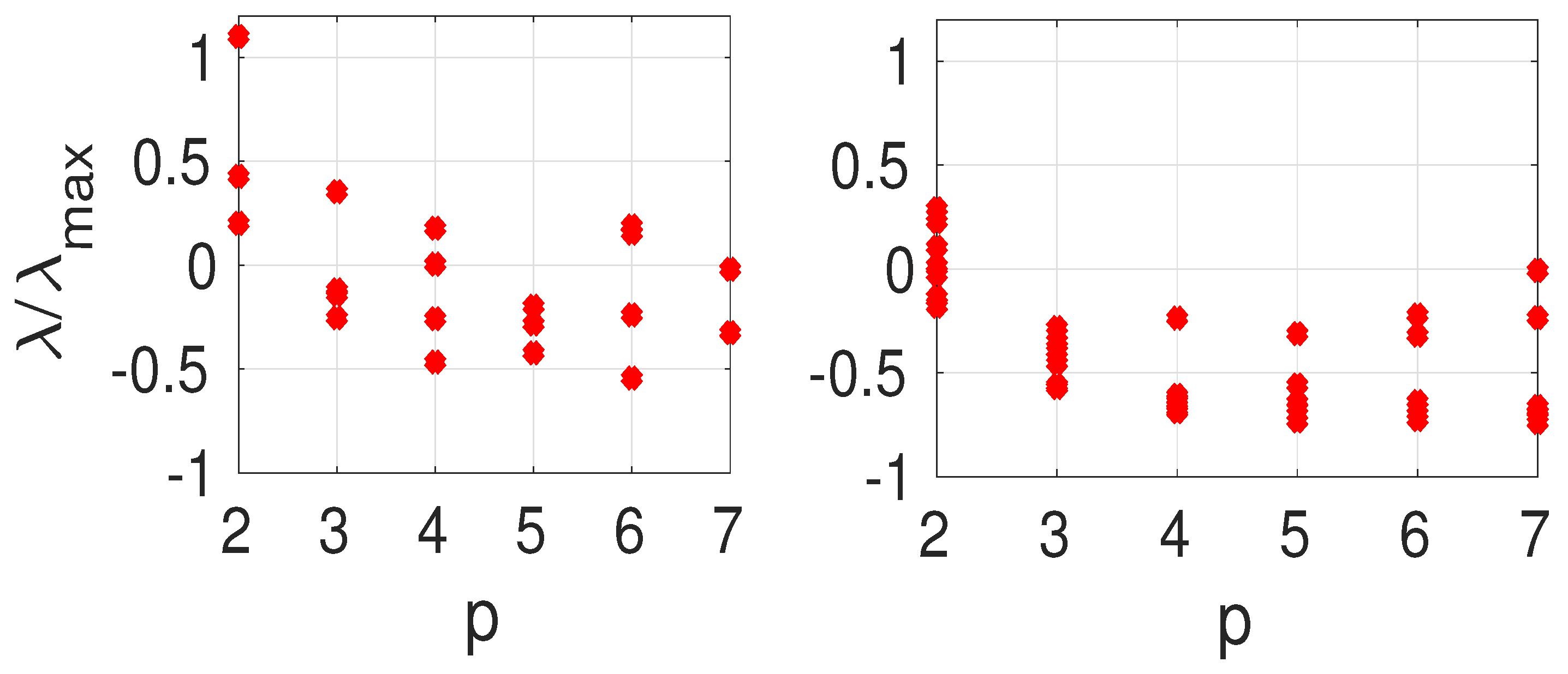
The results shown in the Table 2 and Table 3 are summarized in Figure 4 where we present $\lambda /{\lambda }_{\max }$ vs. the maximal projection (31) for two (left panel) and three (right panel) vaccinated vertices. The normalization factor is

$${\lambda }_{\max }=\left|{\lambda }_{\min }\right|=4{10}^{-2}.$$

As expected from the perturbation theory, $\lambda /{\lambda }_{\max }$ decreases on average when p increases. Exceptions occur when the second-largest projection is on a low-order eigenvector. For example, vaccinating vertices $i=1,j=3$ (left panel) leads to $\lambda /{\lambda }_{\max }=0.2$. The projections of the vector s onto the $V^k, k=2,\dots ,7$ are

$$(0.2836,0.1381,0.0081,0.2295,0.4498,0.0504).$$

The projection is largest for $k=6$ and the second-largest value is for $k=2$. If instead, vertices $i=2,j=5$ are vaccinated, we obtain $\lambda /{\lambda }_{\max }=-0.55$. The projection vector in that case is

$$(0.1814,0.0869,0.2127,0.0038,0.4226,0.3047)$$

whose components are largest for $k=6,7,3,..$, in that order. Theorem 3 explains the difference in $\lambda$ observed for the two situations.

In Figure 4, $\lambda /{\lambda }_{\max }=-1$ is the limit corresponding to a uniform vaccination of the network. We can then compare how vaccinating two or three vertices changes $\lambda$. Figure 4 shows that on average, it is better to vaccinate three vertices rather than two because the values are closer to the limit $\lambda /{\lambda }_{\max }=-1$. The spread in the values of $\lambda /{\lambda }_{\max }$ is also reduced on average for three vaccinated vertices as opposed to two.

4.2. Special Graphs: Complete Graphs and Stars

There are classes of graphs for which choosing $s=\sqrt{n}{V}^k$, with k large, does not affect ${\lambda }^2$. For these graphs, the eigenvalues $-{\omega }_k^2$ are equal so that the ratio

$${\displaystyle \frac{1}{{\omega }_k^2}}{(s,V^k)}^2$$

in the sum (24) does not decrease as k increases.

One example is the class of complete graphs $K_n$.

Definition 5 

(Complete graph $K_n$). A clique or complete graph $K_n$ is a graph where every pair of distinct vertices is connected by a unique edge.

The clique $K_n$ has eigenvalue $-n$ with multiplicity $n-1$ and eigenvalue 0. The eigenvectors for eigenvalue n can be chosen as $v^k=e^1-e^k,k=2,\dots ,n$.

Table 4. Maximal eigenvalue $\lambda$ of M for $S=\mathbf{1}+0.3\sqrt{n}{V}^k$ for complete graphs $K_4, K_5$ and $K_{10}$ from left to right.

k	$\mathit{\lambda }$	k	$\mathit{\lambda }$	k	$\mathit{\lambda }$
2	0.021156	2	0.019695	2	$8.9894{10}^{-3}$
3	0.023520	3	0.019117	3	$9.1072{10}^{-3}$
4	0.021153	4	0.019117	4	$9.1760{10}^{-3}$
		5	0.019117	5	$9.3486{10}^{-3}$
				6	$9.3845{10}^{-3}$
				7	$9.1822{10}^{-3}$
				8	$8.9456{10}^{-3}$
				9	$9.3536{10}^{-3}$
				10	$8.9220{10}^{-3}$

shows the eigenvalue $\lambda$ of M for $K_4, K_5$, and $K_7$ from left to right. As expected there are no significant changes in $\lambda$ as a function of k.

The strategy of vaccinating nodes based on the highest order eigenvector of the Laplacian will fail on complete graphs because the maximal eigenvalue n has multiplicity $n-1$. From another point of view, all vertices behave the same so there are no difference between couples of vertices. Therefore, the network should be vaccinated uniformly to reduce the outbreak.

Another special class of graphs where many eigenvalues are equal are stars. For these, a single vertex, say 1, is connected to the $n-1$ other vertices. The eigenvalues with their multiplicities denoted as exponents are

$$0^1,{(-1)}^{n-2},,{(-n)}^1.$$

The maximal eigenvalue n has multiplicity 1 and therefore we expect the vaccination strategy to work well. Eigenvectors for $-1$ can be chosen as $e^2-e^i(i=3,\dots ,n)$.

• The eigenvector for $-n$ is ${(1,-1/(n-1),\dots ,-1/(n-1))}^T$.
• Table 5. Maximal eigenvalue $\lambda$ of M for $S=\mathbf{1}+0.3\sqrt{n}{V}^k$ for star graphs $n=5, 7$ and 10 from left to right.

  k	$\mathit{\lambda }$	k	$\mathit{\lambda }$	k	$\mathit{\lambda }$
  2	0.10643	2	0.10974	2	0.049159
  3	0.075781	3	0.099318	3	0.055638
  4	0.12306	4	0.10453	4	0.19283
  5	0.019695	5	0.14166	5	0.19283
  		6	0.12715	6	0.19283
  		7	0.014059	7	0.19283
  				8	0.19283
  				9	0.19283
  				10	0.0097722

  shows $\lambda$ as a function of k for $S_5, S_7$ and $S_{10}$.

The results show that the strategy indeed works well in this case. One should vaccinate the center of the star, this can be interpreted as isolating the other vertices.

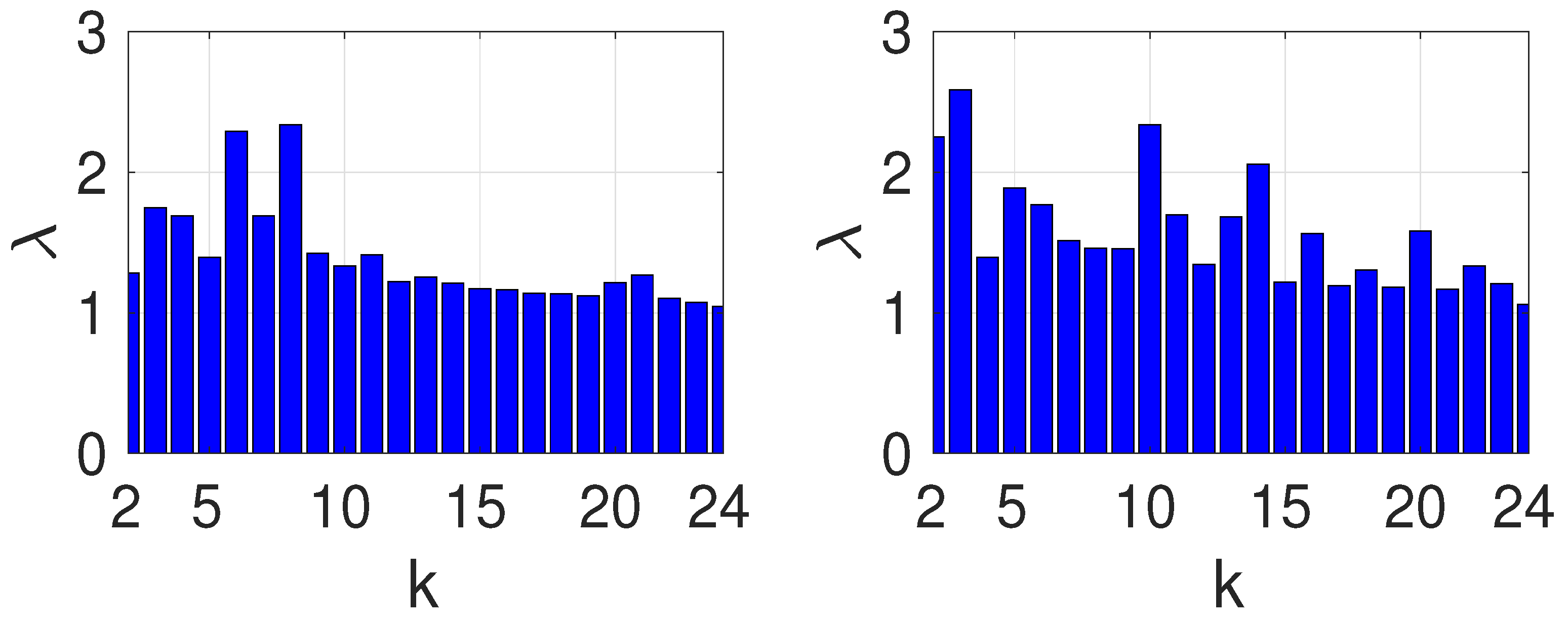
4.3. A More Realistic Case: France

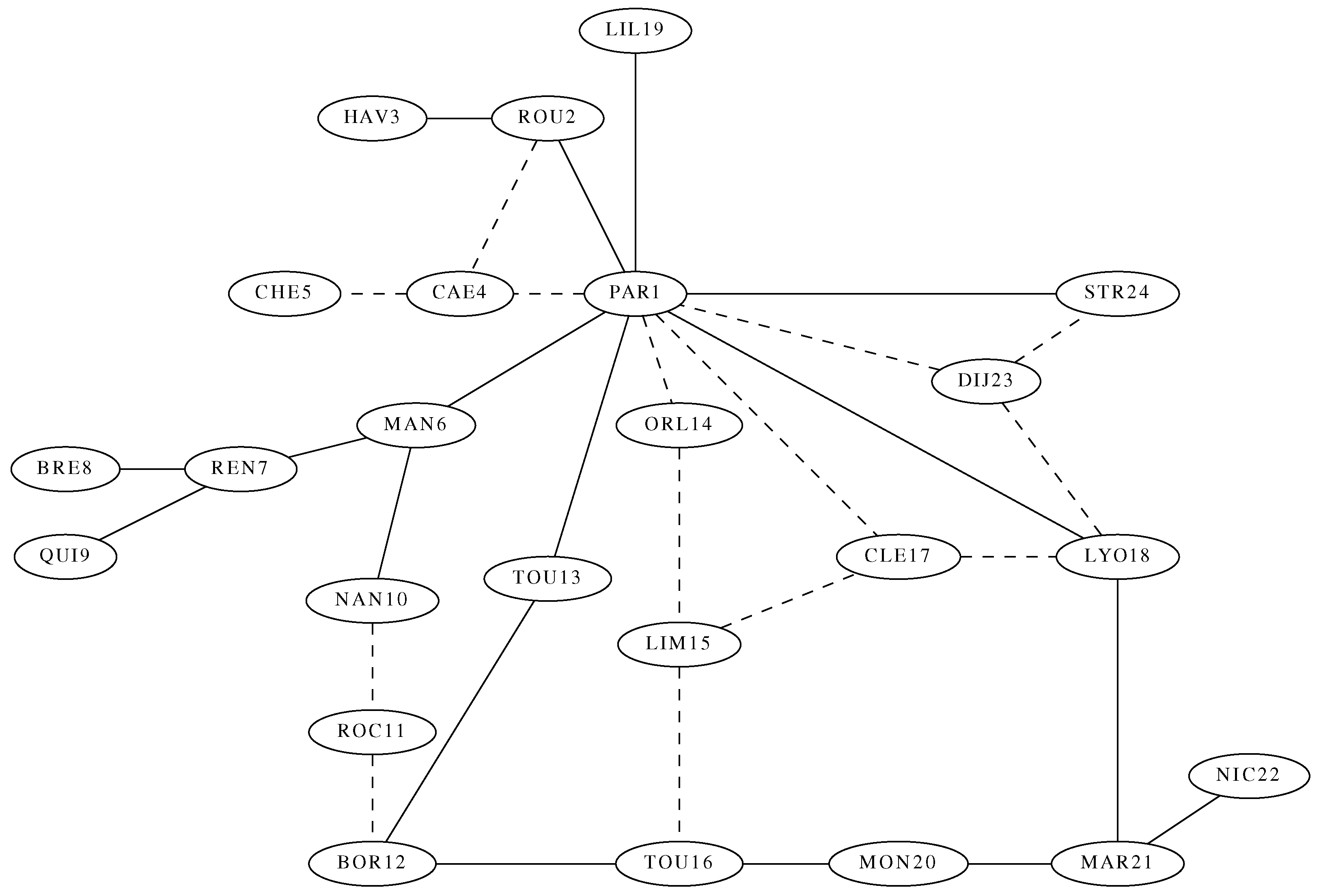
The practical case of vaccinating a whole country can be tackled using our approach. Figure 5 shows a map of the main railway lines in France. The fast lines are presented as continuous edges while the slower ones are dashed. Because of these different mobilities, we need to introduce weights in the Laplacian graph. We chose weights 1 and 0.5 for, respectively, the fast and slow connections. We computed the epidemic growth rate ${\lambda }_k$ for $s=0.3\sqrt{n}{V}^k,k=2,\dots n$ for the parameters $\beta =2, \gamma =1$.

The results are shown in Figure 6 shows ${\lambda }_k$ vs. k for the unweighted and weighted graphs, respectively, on the left and right panels.

For uniform weights, the topology of the graph controls ${\lambda }_k$ so that, as expected, it decays as k increases. There is a factor of 2.3 between the largest and the smallest ${\lambda }_k$.

For the weighted graph (right panel), large eigenvalues occur up to $k=15$. This graph is close to a star with center (PAR1) of highest degree (10); we then expect the results to be close to the ones for stars. Note also the anomalous large $\lambda$ occuring for $V^{10}$ and $V^{14}$. These eigenvectors are localized on vertices 8, 9 and 4, 5 respectively. Despite this, the trend remains that $\lambda$ is smallest for large k.

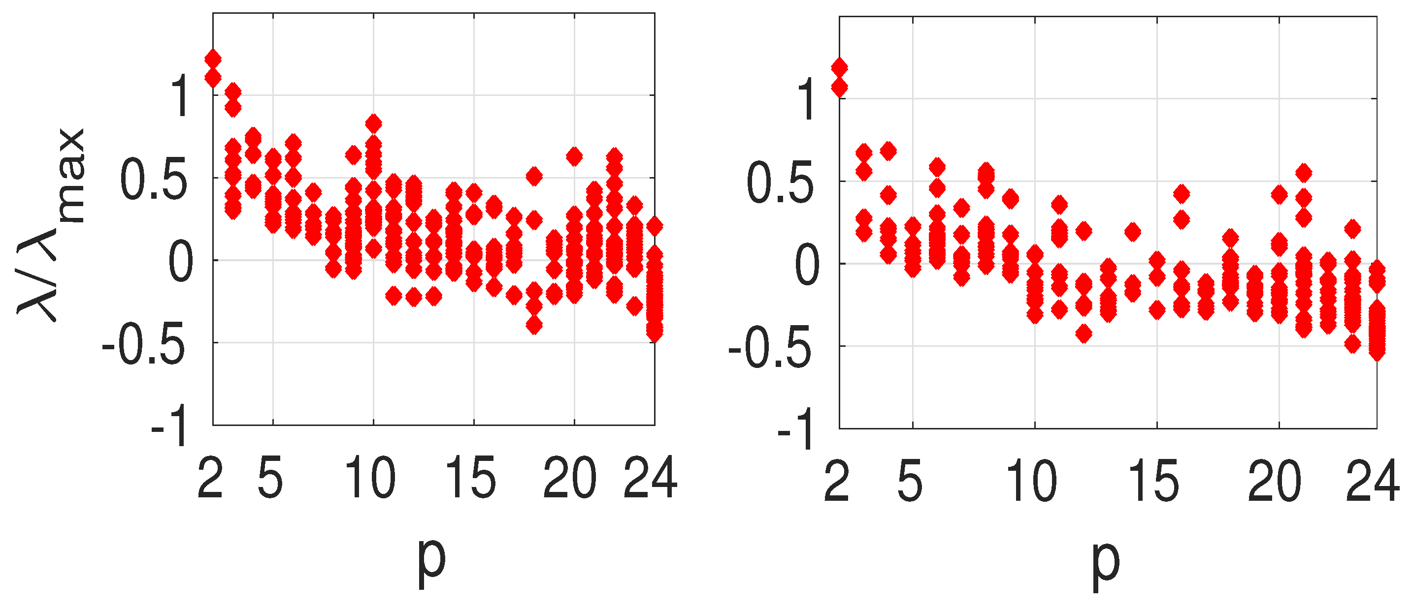
We conclude this section by examining how vaccinating two vertices $i, j$ affects $\lambda$. As above, we chose $s_i=s_j=0.5$. The reference value ${\lambda }_{\min }$ from (30) corresponds to a uniform vaccination, a reduction of s by 1, distributed uniformly over the network. We have

$${\lambda }_{\min }=\beta (1-ϵ{\displaystyle \frac{1}{n}})-\gamma =-0.0129,$$

(32)

where we chose $\beta =1.03$ and $\gamma =1$. We choose ${\lambda }_{\max }=\left|{\lambda }_{\min }\right|$.

The eigenvalue ratio $\lambda /{\lambda }_{\max }$ vs. the projection argument p from (31) is shown in Figure 7 for the weighted (left panel) and unweighted graphs (right panel). As expected, the ratio decreases as p increases. We can reduce the rate of infections significantly so that in some cases it becomes negative and the outbreak is suppressed. Interestingly, the weights do not affect this general qualitative result.

5. SD Slow Diffusion

In this section, we consider that the diffusion parameter $\alpha$ is small compared to the $SI$ term. This was the situation in 2020 when the first wave of the COVID-19 pandemic hit successive different countries after starting in China.

5.1. Perturbation Theory

The epidemic matrix M can be written as

$$M=M_0+\alpha L;M_0=\beta \left(\begin{array}{cccc}{S}_1& 0& \dots & 0\\ 0& S_2& \ddots & ⋮\\ ⋮& \ddots & \ddots & 0\\ 0& \dots & 0& S_n\end{array}\right)-\gamma \mathrm{Id}$$

(33)

The perturbation R of the previous section is L and the perturbation parameter is $\alpha$.

The eigenvalues and eigenvectors of $M_0$ are

$${\lambda }_k^0=\beta S_k-\gamma ,e^k,k=1,2,\dots n$$

(34)

where $e^k$ is the canonical vector of order k. In the absence of diffusion, the maximal eigenvalue of $M_0$ is ${\lambda }_k^0$ where k is such that $S_k$ is maximum. The effect of the diffusion is described by the following theorem:

Theorem 4. 

Let G be a connected graph with n vertices, assume that the number of susceptibles at each vertex i is $S_i$ with a vertex k such that $S_k$ is the only maximum and $S_k-S_j>C\alpha$ for all neighbors j of k ($j\sim k$) where C is a constant. Then the epidemic growth rate is given by

$${\lambda }_k=\beta S_k-\gamma -\alpha d_k-{\displaystyle \frac{{\alpha }^2}{\beta }}\sum _{j\sim k}{\displaystyle \frac{1}{S_k-S_j}}+O\left({\alpha }^3\right),$$

(35)

for $k=1,\dots ,n$, where $d_k$ is the degree of vertex k.

Proof. 

Consider the maximum eigenvalue of $M_0$. We have at order 0 of the perturbation ${\lambda }^0={\lambda }_k^0$ (see (34)) and $v_0^k=e^k$.

In the following, we omit the index k unless it is absolutely necessary. Then, from (9), we have

$${\lambda }_k^1={\displaystyle \frac{(v_0,L{v}_0)}{(v_0,v_0)}}=(e^k,L{e}^k)=-d_k.$$

From (7), the eigenvector $v_1^k$ solves

$$(M_0-{\lambda }^0)v_1^k=({\lambda }^1-L)v_0=({\lambda }^1-L)e^k.$$

Assume $k=1$ for simplicity. Then, the equation above can be rewritten as

$$\left(\begin{array}{cccc}0& 0& \dots & 0\\ 0& S_2-\gamma -{\lambda }^1& \ddots & ⋮\\ ⋮& \ddots & \ddots & 0\\ 0& \dots & 0& S_n-\gamma -{\lambda }^1\end{array}\right)v_1=\left(\begin{array}{c}-d_1\\ 0\\ \ddots \\ 0\end{array}\right)-L{e}^1=\left(\begin{array}{c}0\\ -L_{21}\\ \ddots \\ -L_{n1}\end{array}\right)$$

Then, for general k

$$v_1^k={({\displaystyle \frac{L_{1k}}{\beta (S_1-S_k)}},{\displaystyle \frac{L_{2k}}{\beta (S_2-S_k)}},\dots ,0,\dots ,{\displaystyle \frac{L_{nk}}{\beta (S_n-S_k)}})}^T$$

where the 0 is at position k.

From $v_1^k$, one computes ${\lambda }_k^2$ using (10),

$${\lambda }_k^2=(e^k,L{v}_1^k-{\lambda }^1{v}_1^k).$$

The vectors $e^k$ and $v_1^k$ are orthogonal so that

$${\lambda }_k^2=(e^k,L{v}_1^k).$$

Assume again $k=1$ for clarity, this inner product is

$$(e^1,L{v}_1^1)=\sum _{i=1}^n{e}_i^1\sum _{j=1}^n{L}_{ij}{v_1^1}_j={\displaystyle \frac{L_{12}^2}{\beta (S_2-S_1)}}+{\displaystyle \frac{L_{13}^2}{\beta (S_3-S_1)}}+\cdots +{\displaystyle \frac{L_{1n}^2}{\beta (S_n-S_1)}}$$

$$=\sum _{j\sim 1}{\displaystyle \frac{L_{1j}^2}{\beta (S_j-S_1)}}={\displaystyle \frac{1}{\beta }}\sum _{j\sim 1}{\displaystyle \frac{1}{S_j-S_1}}$$

because $L_{1j}=1$ if $j\sim 1$ and zero otherwise. It is then easy to obtain ${\lambda }_k^2$ for general k.

□

We can make the following comments:

• The first order in the perturbation comes from the degree. Then, for equal $S_k$, a vertex with a larger degree will yield a smaller $\lambda$.
• The influence of neighbors appears at the second order with the term $S_k-S_j$ in the denominator. When $S_k-S_j$ is small, this term can be large and the approximation breaks down. One should then use the approach FD.

5.2. Illustration on the Graph with Seven Vertices

To illustrate these calculations, we consider the seven-vertex graph shown in Figure 1. We chose $\alpha =0.3,\beta =9,\gamma =6$ and

$$S={\left(0.50.90.50.50.50.50.5\right)}^T.$$

Table 6. Epidemic growth rate $\lambda$ when $S_k=0.9$ for k shown on first column. The second, third, fourth and fifth columns are, respectively, the degree, first order, second order and exact calculations.

Vertex k	Degree	${\mathit{\lambda }}^0+\mathit{\alpha }{\mathit{\lambda }}^1$	${\mathit{\lambda }}^0+\mathit{\alpha }{\mathit{\lambda }}^1+{\mathit{\alpha }}^2{\mathit{\lambda }}^2$	Exact $\mathit{\lambda }$
1	3	1.2	1.275	1.28
2	2	1.5	1.55	1.55
3	3	1.2	1.275	1.28
4	2	1.5	1.55	1.55
5	3	1.2	1.275	1.28
6	2	1.5	1.55	1.55
7	1	1.8	1.825	1.823

shows the epidemic growth rate when $S_k=0.9$ together with its degree and the first and second orders of perturbation. We change $S_k$ following a circular permutation. The order 0 is

$$\beta S_k-\gamma \approx 2.1$$

One sees that the perturbation approach is in excellent agreement with the exact calculations. As the degree decreases from 3 to 1, the eigenvalue increases from 1.28 to 1.82.

To see the effect of vaccination, we reduced the maximum $S_k$ from 0.9 to 0.8 and recomputed $\lambda$. The order 0 is

$$\beta S_k-\gamma \approx 1.2.$$

The results are shown in

Table 7. Same as Table 6 except $S_k=0.8$. The rows have been sorted to have $\lambda$ in increasing order.

Vertex k	Degree	${\mathit{\lambda }}^0+\mathit{\alpha }{\mathit{\lambda }}^1$	${\mathit{\lambda }}^0+\mathit{\alpha }{\mathit{\lambda }}^1+{\mathit{\alpha }}^2{\mathit{\lambda }}^2$	Exact $\mathit{\lambda }$	$\frac{\mathbf{\Delta }\mathit{\lambda }}{\mathit{\lambda }}$
1	3	0.3	0.4	0.41	0.68
3	3	0.3	0.4	0.41	0.68
5	3	0.3	0.4	0.41	0.68
2	2	0.6	0.67	0.67	0.55
4	2	0.6	0.67	0.66	0.55
6	2	0.6	0.67	0.67	0.55
7	1	0.9	0.93	0.93	0.50

.

Note again the excellent agreement between the perturbation theory and the exact calculation. For this simple situation, $\lambda$ is fixed by the degree of the vertex. The rows have been sorted out in descending degree and one sees that $\lambda$ increases as the degree decreases. To compare the situations $S_{max}=0.9$ and $S_{max}=0.8$ we plot in the last column

$${\displaystyle \frac{\Delta \lambda }{\lambda }}={\displaystyle \frac{{\lambda }_{S=0.9}-{\lambda }_{S=0.8}}{{\lambda }_{S=0.9}}}.$$

This quantity decreases from $0.68$ for degree 3 to 0.5 for degree 1. It is therefore best to vaccinate high-degree vertices.

When the distribution of S is not uniform, for the same degree, $\lambda$ will depend on the neighbors j of k through the term $S_k-S_j$. The epidemic growth rate will be smaller for vertices k where $S_k-S_j$ small and larger otherwise.

6. Conclusions

We studied a vaccination policy on a simple model of an epidemic on a geographical network by examining the maximum eigenvalue $\lambda$ of a matrix formed by the susceptibles and the Laplacian graph matrix L: the epidemic growth rate. For that, we analyzed the epidemic matrix M using perturbation theory.

When mobility and disease dynamics have similar time scales (case FD), the zero-order eigenvector is the first eigenvector of the Laplacian graph. The epidemic grows uniformly on the network and we found that it is most effective to “vaccinate” the network uniformly. If this is not possible, then it is best to vaccinate two or more vertices that follow the eigenvector of L of highest order $V^n$. For this strategy to hold, the multiplicity of the maximal eigenvalue should be small. For a complete graph $K_n$, the eigenvalue n has multiplicity $n-1$ and the vaccination strategy breaks down. This criterion depends on the structure of the graph, not on its size. We therefore expect it to occur on arbitrary size networks.

To design strategies to reduce the spread of the infection, we illustrate these results with a general graph of seven vertices and eight edges and a graph of the main railway lines of France. We show that, on average, it is better to vaccinate three vertices rather than two. These vertices should have a maximal projection on a high-order eigenvector to reduce the epidemic growth rate.

The second limit SD is when the local disease dynamics is faster than the mobility. Then, the epidemic grows locally on the vertex k where $S_k$ is maximum. The perturbation theory shows that it is most effective to vaccinate high degree vertices and not neighbors.

These results answer the questions of the introduction as to the role of the degree, which vertex or vertices to vaccinate, the influence of the eigenvectors of the Laplacian, etc. They show the importance of the topology of the network and the spectral properties of the Laplacian graph in the dynamics of the disease.

From a public health point of view, to implement the strategy suggested in this work, we should consider the following main two factors: how fast the disease dissemination is, and what the main connections between the cities are.