CS-MLAkNN: A Cost-Sensitive Adaptive k-Nearest Neighbors Algorithm for Imbalanced Multi-Label Learning

Abstract

Multi-label data usually carries a complex structural class imbalance, which significantly affects the overall predictive performance of multi-label learning models. Although many studies have investigated this problem, most existing methods rely on resampling, static cost weighting, or ensemble learning. Few studies simultaneously consider cost information and neighborhood size within the local statistical model of ML-kNN. To address this issue, this paper proposes a cost-sensitive adaptive k-nearest neighbors algorithm, named CS-MLAkNN, for imbalanced multi-label learning. The algorithm implements a dual cost-sensitive strategy at both the feature and label levels within the ML-kNN framework. Specifically, feature-level cost sensitivity is achieved through distance weighting during the training phase. In the prediction phase, label distribution information is incorporated into the posterior probability calculation to achieve label-level cost sensitivity. Moreover, the optimal number of neighbors (k) is determined adaptively through cross-validation. CS-MLAkNN maintains the simplicity and interpretability of the original ML-kNN, and meanwhile it explicitly introduces cost sensitivity and adaptiveness into three key steps: distance metric, posterior decision, and neighbor determination. Experimental results on 14 benchmark datasets demonstrate that the proposed method achieves optimal or near-optimal performance across various evaluation metrics. It also shows significant advantages over other state-of-the-art imbalanced multi-label learning algorithms.

1. Introduction

Supervised learning constitutes a cornerstone of machine learning. Its primary objective is to induce a mapping function from input features to output targets using labeled data, thereby minimizing prediction errors and aligning predictions with ground-truth labels [1]. In conventional tasks such as image recognition [2], text classification [3], and medical diagnosis [4], the dominant approach is Single-Label Learning (SLL) [5]. In this paradigm, each instance is assigned to a unique, mutually exclusive category. Consequently, both optimization objectives and evaluation metrics focus on selecting a single class from a candidate set. Although SLL has achieved substantial success, its underlying assumption—that an instance corresponds to a single semantic concept—often oversimplifies real-world data complexities. To address this limitation, Multi-Label Learning (MLL) was introduced [6]. Unlike SLL, MLL allows each instance to be associated with a set of labels simultaneously. This paradigm aligns more closely with practical scenarios. For instance, an image may depict trees, clouds, grassland, mountains, sky and lakes (see Figure 1); a news report may cover politics and military affairs; and a medical diagnosis may reveal multiple pathological indicators.

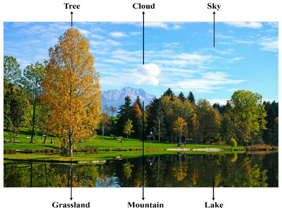
Figure 1. An example of a multi-label image.

Let $X={\mathbb{R}}^d$ be a d-dimensional feature space and $Y=\{y_1,y_2,\dots ,y_L\}$ be an L-dimensional label space. Multi-label learning can be formulated as training a function model $f:X\to 2^Y$ on the training set $D={\left\{\left(x_i,y_i\right)\right\}}_{i=1}^N$, where $x_i\in {\mathbb{R}}^d$ represents a d-dimensional input instance and $Y_i\in Y$ denotes the corresponding label set. For any test instance $x^{\prime }$, the trained function model $f$ will output its predicted label set $Y^{\prime }=f\left(x^{\prime }\right)$. Similar to traditional single-label learning, multi-label learning also faces the issue of class imbalance, which is more complex in this context. Specifically, class imbalance in multi-label data manifests in three aspects [7]: within individual labels, across labels, and among label subsets. Within-label imbalance refers to the fact that positive instances are often much fewer than negative ones within a specific label, while across-label imbalance occurs when the number of positive instances significantly varies across labels. Additionally, some label subsets appear more frequently due to the influence of label semantics, leading to label subset imbalance. These imbalances are commonly found in multi-label datasets, even those of relatively small sizes.

It is well known that single-label class imbalance severely reduces the recognition performance of minority classes. In multi-label learning, various imbalance phenomena combine and become more complex. This situation further decreases model performance. To address this problem, researchers focus on two main issues: first, how to measure the degree of class imbalance in multi-label data and second, how to develop algorithms to handle this imbalance. Specifically, due to the expansion of the label space, traditional methods for single-label datasets are no longer suitable. Consequently, researchers have developed several methods specific to multi-label learning. These include early general metrics, such as $Card$ and $Dens$ [8], and specialized methods for ML-CIL, such as $IR$ and $MeanIR$. The calculation formulas are as follows:

$$Card={\sum }_{i=1}^N{\displaystyle \frac{\left|Y_i\right|}{N}}$$

(1)

$$Dens=Card/L$$

(2)

$${IR}_l={\displaystyle \frac{\left|R_{max}\right|}{\left|R_l\right|}}$$

(3)

$$MeanIR={\displaystyle \frac{1}{L}}{\sum }_{l=1}^L{IR}_l$$

(4)

Table 1 presents the class imbalance characteristics of 14 benchmark multi-label datasets. As indicated in the table, the class imbalance problem is prevalent across these datasets. Notably, the medical dataset exhibits a significantly higher imbalance level than the others. In contrast, the flag dataset shows a relatively lower level of imbalance.

Table 1. Characterization of imbalance level.

Datasets	$\mathit{C}\mathit{a}\mathit{r}\mathit{d}$	$\mathit{D}\mathit{e}\mathit{n}\mathit{s}$	$\mathit{M}\mathit{e}\mathit{a}\mathit{n}\mathit{I}\mathit{R}$
emotions	1.868	0.311	2.320
flags	3.392	0.485	1.859
medical	1.245	0.028	328.069
enron	3.378	0.064	136.862
yeast	4.237	0.303	8.579
scene	1.074	0.179	4.662
genbase	1.252	0.046	143.458
bio3	1.162	0.145	3.496
image	1.237	0.247	3.116
birds	1.014	0.0534	32.859
foodtruck	1.935	0.161	8.788
PlantPseAAC	2.134	0.178	21.879
CAL500	26.044	0.150	22.266
water-quality-nom	5.073	0.362	2.021

The precise characterization of class imbalance in multi-label data has facilitated the development of specialized algorithms, effectively addressing the second issue mentioned above. Generally, existing solutions for multi-label class imbalance can be categorized into four groups: sampling strategies, cost-sensitive learning, threshold moving, and ensemble learning. Sampling strategies aim to rebalance the class distribution of the training set by synthesizing or removing instances. Representative algorithms include ML-SOL, MLUL, and MLONC [9,10]. Cost-sensitive learning assigns different penalty weights at the classifier level to emphasize minority class instances, as exemplified by LW-ELM [11]. Threshold moving serves as a post-processing technique that adjusts the decision threshold to an optimal position after the model is trained, such as CCkEL [12]. As for ensemble learning, it integrates multiple strategies to achieve robust classification performance. Typical examples include ECC++ and COCOA [13,14]. Although these methods have improved prediction performance for minority labels, they face inherent limitations particularly within the context of k-nearest neighbor frameworks. While some cost-sensitive kNN variants exist, they predominantly rely on global static weights or adjust costs only at the decision boundary, neglecting the cost information embedded in the feature structure. Most critically, traditional kNN-based imbalanced learning algorithms [15,16] typically employ a fixed number of neighbors for all query instances. This rigid approach fails to adapt to the varying local densities of minority and majority classes, often resulting in minority instances being overwhelmed in a fixed-size neighborhood.

To address these challenges and bridge the gap in current kNN-based methodologies, this paper proposes a systematic framework named CS-MLAkNN. Unlike existing static weighted kNN methods, CS-MLAkNN constructs a unified framework that dynamically integrates cost information with neighborhood adaptiveness. Specifically, this framework distinguishes itself through a structured improvement mechanism:

(1)

It implements a feature-level cost-sensitive strategy by reshaping the local neighborhood structure via distance weighting to ensure that selected neighbors are more informative for minority classes.

(2)

It incorporates a label-level cost-sensitive strategy during posterior probability estimation to explicitly amplify the decision weight of minority labels.

(3)

It introduces a global adaptive mechanism to determine the optimal neighbor size via cross-validation, thereby overcoming the performance bottleneck caused by fixed neighbor settings in varying data distributions.

Extensive experiments on 14 benchmark multi-label imbalanced datasets demonstrate the superiority of the proposed method. The results indicate that CS-MLAkNN achieves optimal or near-optimal performance across six evaluation metrics. Moreover, statistical analyses and ablation studies further validate the robustness and effectiveness of the algorithm.

The rest of this paper is organized as follows. Section 2 reviews related work on multi-label class imbalance learning. Section 3 introduces ML-kNN, along with the incorporation of instance-level cost, label-level cost, and global adaptive neighbor selection, and provides a detailed flow of CS-MLAkNN; Section 4 presents the datasets, experimental settings, the results of comparative experiments and ablation experiments, and various analyses; and Section 5 concludes the paper with a summary.

2. Related Work

In recent years, class imbalance learning has established a well-developed theoretical framework within the single-label domain. Generally, existing approaches can be categorized into four groups. First, sampling methods aim to rebalance the class distribution of the training set. Common techniques include random undersampling, random oversampling, and synthesizing minority class samples [17]. Second, cost-sensitive learning assigns higher misclassification costs to minority classes in the loss function. This strategy compels the model to focus more on the minority class [18]. Third, threshold moving strategies adjust the decision threshold of soft-output models. By shifting the threshold to favor the minority class, these methods correct the bias caused by imbalanced data distributions. Finally, ensemble learning integrates one or more of the aforementioned strategies into a unified framework to enhance the overall performance [19].

Sampling represents the most intuitive approach to address class imbalance. It balances the training set by either replicating minority class samples or removing majority class samples. Based on random undersampling (RUS) and random oversampling (ROS) Charte et al. [8,20] proposed the ML transformation strategy. This strategy treats each label independently. By comparing the $IR$ and $MeanIR$ of each label, the method classifies them into majority or minority classes. Subsequently, the ML-ROS algorithm clones instances associated with minority class labels, while ML-RUS removes instances containing majority class labels. However, the ML transformation strategy suffers from a critical limitation. Since a single instance may simultaneously contain both majority and minority class labels, sampling based on a single label inevitably alters the distribution of other concurrent labels. To address this issue, Charte et al. [20] proposed an improved algorithm named ML-SMOTE. This method combines ML transformation with the SMOTE technique. It redefines the concept of neighborhoods in the multi-label space and synthesizes new instances near minority label samples. Subsequently, researchers focused on local label imbalance characteristics. Representative methods include MLSOL and MLUL. These algorithms generate diverse synthetic instances or remove harmful samples by measuring the $IR$ of each label within local regions. More recently, DR-SMOTE [17] emphasized the diversity and reliability of synthetic samples within the SMOTE framework. Similarly, MLONC [10] utilizes natural neighbors and label correlations to adaptively determine the oversampling neighborhood. This approach enhances the local representation of minority label samples. Despite these advancements, sampling methods still face inherent limitations. First, precisely defining “positive/negative samples” and “neighborhoods” in the multi-label space remains challenging. Improper definitions may introduce noise or disrupt the original local structure. Second, hyperparameters in the underlying classifier, such as the number of neighbors, often remain static before and after sampling. Consequently, these methods lack fine-grained adjustments optimized for specific evaluation metrics.

Cost-sensitive learning represents another pivotal approach for addressing class imbalance. The core principle involves assigning distinct penalty weights to misclassifications of different classes within the loss function. Consequently, the optimization process naturally biases the model towards the minority class. In the field of multi-label learning, the Label-Weighted Extreme Learning Machine (LW-ELM) [11] serves as a representative example. Operating within the ELM framework [21,22], it handles each label independently. By assigning specific weights to positive and negative instances based on imbalance ratios, the algorithm compels the model to prioritize minority labels during error calculation. Another line of research combines cost-sensitive learning with neighborhood-based lazy learning [23]. For instance, BRWDkNN [24] learns a set of weights for each training prototype within the Binary Relevance framework. It adjusts the influence of neighboring prototypes via weighted distance metrics. Furthermore, this method extends the traditional classification error rate to imbalance-sensitive metrics, such as multi-label $F_{macro}$, to enhance performance on long-tail labels. Its stacked extension, MWBRWDNN [25], integrates WDNN [26] into the secon7d layer of the Meta-BR structure. This method weights the label features predicted by the first layer. As a result, it assigns varying importance to different labels and their combinations at the feature level, effectively capturing label correlations and enhancing imbalance robustness. In summary, existing cost-sensitive learning methods typically rely on global static weights or indirect objective function adjustments within the BR framework [27]. However, they generally lack a unified mechanism to co-optimize cost modeling with structural hyperparameters, such as neighbor size, particularly within local statistical models like ML-kNN.

In multi-label learning, threshold moving techniques serve as another effective strategy for addressing imbalanced data distributions [28]. The Optimized Threshold (OT) algorithm [29] is a representative application of this category. Generally, the operation of OT consists of two stages. First, a specific decision threshold is independently determined for each label in the dataset. Second, during the prediction phase, the model’s output probability is compared with the corresponding threshold to determine the final label assignment. Regarding the determination of these thresholds, Read et al. [30] proposed two main approaches. The first relies on domain knowledge for empirical specification, while the second utilizes cross-validation for data-driven optimization. It is worth noting that OT and similar methods primarily focus on the posterior calibration of output probabilities at the decision level. They do not alter the internal mechanisms of the learner, such as neighborhood construction or probability estimation, during the training phase.

Ensemble learning has been extensively employed to address class imbalance in multi-label scenarios [14]. The fundamental principle involves constructing multiple base classifiers and aggregating their outputs during prediction. This process improves both the stability and generalization capability of the model. Representative approaches include the Ensemble of Classifier Chains (ECC) and the Random k-Labelsets (RAkEL) [31].

Specifically, ECC explicitly models higher-order label correlations. It achieves this by generating random label permutations and utilizing the predictions of preceding labels as input features for subsequent classifiers. While RAkEL divides the original label set into smaller subsets and trains a multi-class classifier for each one. This strategy effectively captures the label combination structure within label subspaces. Further, to simultaneously address class imbalance and label correlations, methods such as COCOA [14] introduce a cost-sensitive mechanism. This algorithm trains multiple binary or multi-class learners on different label subspaces. Subsequently, it weights their outputs in the ensemble layer to enhance the prediction performance for minority labels. Through label decomposition and structural fusion, these ensemble methods significantly improve performance on multi-label imbalanced data. However, they typically require training and maintaining a large number of base classifiers, often treating them as “black boxes.” Consequently, they lack the ability to integrate cost modeling, local statistics, and neighbor size adjustments within a single, unified neighborhood model [32].

In summary, the review above indicates that current methods for addressing class imbalance in multi-label learning primarily focus on data-level resampling, static cost weighting, threshold post-processing, or complex ensemble frameworks. However, these approaches often treat base learners as “black boxes.” Consequently, they lack a systematic characterization of cost modeling and neighborhood structures within local statistical models, such as ML-kNN. Specifically, a critical unresolved issue is how to jointly consider sample and label costs, local neighborhood statistics, and neighbor sizes within a single unified model. Furthermore, the optimization process must align with imbalance-sensitive metrics, such as $F_{macro}$. To address these challenges, this paper proposes a systematic framework named CS-MLAkNN (Cost-Sensitive and Neighbor-Size Adaptive Multi-Label k-Nearest Neighbor). Built upon the classic ML-kNN paradigm, this method directly integrates cost information into the probability estimation and neighborhood construction processes. Additionally, it employs a mechanism to automatically select an appropriate k-value.

3. Methods

This section first provides a brief introduction to the theory and methods of ML-kNN, followed by a detailed explanation of the proposed CS-MLAkNN algorithm and its pseudocode.

3.1. ML-kNN

ML-kNN [15] is a classic lazy learning algorithm derived from the traditional k-Nearest Neighbors (kNN) method. It employs the Maximum A Posteriori (MAP) principle to determine label sets based on the statistical information of neighbors. Specifically, for a test instance $x$, the algorithm identifies its $k$ nearest neighbors in the training set, denoted as $N\left(x\right)$. For each label $l$, let $E_l\in \left\{\mathrm{0,1},\dots ,k\right\}$ represent the number of neighbors belonging to the positive class. ML-kNN estimates the prior probabilities $P\left(H_l\right)$ and the conditional likelihoods $P\left(E_l\right|H_l)$ from the training data, where $H_l\in \left\{\mathrm{0,1}\right\}$ denotes whether the instance actually possesses label $l$.

Based on these statistics, the posterior probability $P(H_l=1|E_l)$ is computed using Bayes’ theorem. If $P(H_l=1|E_l)>P(H_l=0\left|E_l\right)$, the label $l$ is assigned to the instance [15]. While ML-kNN offers simplicity and interpretability, it relies on a fixed $\mathrm{k}$ and assigns equal weight to all neighbors. These assumptions are ill-suited for imbalanced multi-label data, where minority class instances are easily overwhelmed by majority class neighbors. Furthermore, standard ML-kNN fails to account for the varying costs associated with misclassifying different labels. These limitations necessitate the cost-sensitive and adaptive improvements proposed in our CS-MLAkNN.

3.2. CS-MLAkNN

Motivated by these challenges, we propose CS-MLAkNN: a cost-sensitive adaptive k-nearest neighbors algorithm for imbalanced multi-label learning. It is well known that cost-sensitive learning methods are classifier-dependent [11]. Therefore, we made three improvements to ML-kNN. First, we introduced a cost-sensitive strategy at the feature level by characterizing the neighborhood structure’s weights. Second, we incorporated a cost-sensitive strategy at the label level by considering the class imbalance in the calculation of posterior probabilities. Finally, we made k adaptive.

To effectively handle the local data distribution of different semantics, we propose a Label-Specific Prototype Weighting mechanism. Unlike traditional methods that learn a global distance metric for all classes, our approach learns a weight matrix $W\in {\mathbb{R}}^{L\times N}$, where each entry $w_{l,i}$ represents the specific importance of the $i$-th training instance with respect to the $l$-th label. Although the weights are instance-specific, they are optimized globally for each label to maximize the overall classification performance. Specifically, for a given label $l$, we aim to find the optimal weight vector $w_l=\left[w_{l,1},w_{l,2},\dots ,w_{l,N}\right]$ that maximizes the $F_{macro}$ on the training data. The distance between a query instance and a prototype $x_i$ is scaled by $w_{l,i}$ as defined in Equation (5):

$$d_w\left(q,x_i\right)={\displaystyle \frac{d\left(q,x_i\right)}{w_{l,i}}}$$

(5)

where $w_i>0$, and $d(q,x_i)$ represents the traditional distance calculation method. For example, using the Euclidean distance $d_E$, we have

$$d\left(q,x_i\right)=d_E\left(q,x_i\right)=\sqrt{{\sum }_{j=1}^D{{(q}_j-x_{ij})}^2}$$

(6)

As previously discussed, we employ confusion matrix-based evaluation metrics to construct the objective function. To derive the weight matrix $w$, we utilize an extended version of the Prototype Weighting (PW) method [24]. The rationale for this specific formulation lies in directly optimizing imbalance-sensitive evaluation metrics (e.g., $F_{macro}$) which are typically non-differentiable. To address this, we employ a sigmoid-based smooth approximation to construct a differentiable objective function. The theoretical validity of explicitly embedding cost-sensitive mechanisms into the optimization objective has been well-established in previous works. For instance, the Label-Weighted Extreme Learning Machine (LW-ELM) [11] demonstrated that assigning class-dependent weights within the objective function significantly reduces the bias towards majority classes. Furthermore, to ensure numerical stability during the optimization process, the settings of key hyperparameters in our framework—specifically the smoothing factor $\mathrm{s}$ and the learning rate $\eta$—follow the empirical recommendations derived from the convergence analysis presented in [11]. Inspired by this theoretical foundation, the determination of $w$ is formulated as an optimization problem, defined as follows:

$$w^{\ast }={\arg \mathrm{m}\mathrm{a}\mathrm{x}}_w V(w,f(x),y)$$

(7)

Here, V(·) denotes a confusion-matrix-based evaluation metric, with larger values indicating better classifier performance (for example, F_macro). Rastin et al. [24] proposed an optimization-based generalization of the confusion matrix, Objective Generalization of PW, which enables solving the optimization problem presented here. The confusion matrix comprises four basic counts: True Positives ($TPs$), True Negatives ($TNs$), False Positives ($FPs$), and False Negatives ($FNs$), which are the basic metrics used in many objectives (e.g., classification accuracy/error rate, G-mean, F-score, precision, recall, sensitivity, and specificity). The $FPs$ and $FNs$ metrics count incorrectly classified negative and positive samples, respectively, and can be obtained by summing the classification losses over negative and positive samples alone. Following the reference [25], these losses are defined in Equations (8)–(11).

$${TP}_l=|x_l^{+}|-{\sum }_{x^{+}\in X_l^{+}}\left[e\left(x^{+}\right)\right]={\sum }_{x^{+}\in X_l^{+}}{\phi }_{\beta }\left(r{\left(x^{+}\right)}^{-1}\right)$$

(8)

$${FN}_l={\sum }_{x^{+}\in X_l^{+}}\left[e\left(x^{+}\right)\right]$$

(9)

$${FP}_l={\sum }_{x^{-}\in X_l^{-}}\left[e\left(x^{-}\right)\right]$$

(10)

According to [25], we have

$$e(x)\approx \phi (r(x))={\displaystyle \frac{1}{1+e^{\beta (1-r(x\left)\right)}}},r(x)={\displaystyle \frac{d_w(x,x^{=})}{d_w(x,x^{\ne })}}$$

(11)

where $x^{=}$ and $x^{\ne }$ denote the nearest neighbors of $x$ from the same class and different classes, respectively. Meanwhile, $X_l^{+}$ and $X_l^{-}$ represent the positive and negative instance sets for the $l$-th label. Based on these definitions, the transformation process described in Equation (12) is established. Similarly, the analytical definition of $TNs$ can be derived. Consequently, any objective function based on the confusion matrix can be formulated. Taking the $F_{macro}$ as an example, we have

$$F_{macro}={\displaystyle \frac{1}{L}}{\sum }_{l=1}^L{F}_L={\sum }_{l=1}^L{\displaystyle \frac{2{TP}_l}{2{TP}_l+{FP}_l+{FN}_l}}$$

(12)

The weight matrix update function is shown in Equation (13)

$$w_{j,l}^{new}=w_{j,l}^{old}+\eta {\displaystyle \frac{\partial F}{\partial w_{j,l}}}$$

(13)

where

$${\displaystyle \frac{\partial F}{\partial w_{j,l}}}=2{\displaystyle \frac{\hspace{0.17em}{TP}_{l^{\prime }}{FP}_l-{FP}_{l^{\prime }}{TP}_l+\hspace{0.17em}{TP}_{l^{\prime }}{FN}_l-{FN}_{l^{\prime }}{TP}_l}{(2{TP}_l+{FP}_l+{FN}_l{)}^2}}$$

(14)

$${{TP}_l}^{\prime }=-{\sum }_{x^{+}\in X_l^{+}}{{\phi }^{\prime }}_{\beta }\left(r{\left(x^{+}\right)}^{-1}\right){\displaystyle \frac{r{\left(x^{+}\right)}^{\prime }}{r{\left(x^{+}\right)}^2}}$$

(15)

$${{FN}_l}^{\prime }={\sum }_{x^{+}\in X_l^{+}}{{\phi }^{\prime }}_{\beta }\left(r\left(x^{+}\right)\right)r{\left(x^{+}\right)}^{\prime }$$

(16)

$${{FP}_l}^{\prime }={\sum }_{x^{-}\in X_l^{-}}{{\phi }^{\prime }}_{\beta }\left(r\left(x^{-}\right)\right)r{\left(x^{-}\right)}^{\prime }$$

(17)

$$r{\left(x\right)}^{\prime }=r(x)w_j\left[{\left({\displaystyle \frac{x_j-x_j^{=}}{d(x,x^{=})}}\right)}^2-{\left({\displaystyle \frac{x_j-x_j^{\ne }}{d(x,x^{\ne })}}\right)}^2\right]$$

(18)

During the probability estimation and prediction stages, CS-MLAkNN further incorporates a label-level cost-sensitive strategy. This strategy is integrated into the calculation of posterior probabilities based on the label distribution of the training set. Specifically, the algorithm assigns cost coefficients according to the imbalance level of each label. This mechanism effectively amplifies the positive class probability of minority labels during the posterior decision process (as illustrated in Figure 2b). Let $R_l$ denote the number of positive samples for the $l$-th label in the training set. The imbalance level is defined as

$${IR}_l={\displaystyle \frac{\left|R_{max}\right|}{\left|R_l\right|}}$$

(19)

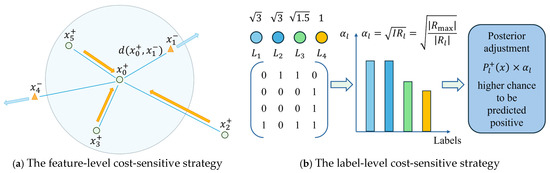
Figure 2. Cost-sensitive mechanisms of CS-MLAkNN.

The larger ${IR}_l$ is, the rarer the positive instances for that label, and the higher the cost of misclassification. To reflect this, we introduce a cost coefficient ${\alpha }_l$ for each label:

$${\alpha }_l=\sqrt{{IR}_l}$$

(20)

In the prediction phase, we first obtain the original posterior probabilities $P(H_l=1\mid E_l=e)$ and $P(H_l=0\mid E_l=e)$ for the $l$-th label. Subsequently, we amplify the posterior probability of the positive class. The formulation is given by

$$\tilde{P}\left(H_l=1∣E_l=e\right)={\alpha }_l\times P(H_l=1\mid E_l=e)$$

(21)

Subsequently, the amplified positive probabilities are normalized alongside the negative class probability $P(H_l=0\mid E_l=e)$. The final classification decision is determined based on these normalized outputs. Notably, when the cost-sensitive mechanism is disabled, the algorithm sets the weight matrix $W$ to an identity matrix and the cost coefficients ${\alpha }_l=1$ to 1. Under these conditions, CS-MLAkNN mathematically reduces to the standard ML-kNN algorithm.

In the ML-kNN algorithm, the hyperparameter $\mathrm{k}$ significantly impacts the model’s performance [33]. For multi-label imbalanced datasets, an excessively small $\mathrm{k}$ increases sensitivity to noise. Conversely, an overly large $\mathrm{k}$ leads to over-smoothing, which may obscure subtle differences between labels. Therefore, selecting an appropriate $\mathrm{k}$ is crucial for achieving optimal classification results. To determine the optimal neighborhood size $\mathrm{k}$ without introducing data leakage, we implement a strict Inner Cross-Validation (Inner CV) procedure. The training set is first partitioned into equal-sized internal folds (e.g., 5 folds). We then define a candidate search range $\mathrm{K}$ for the neighborhood size. For each candidate $k\in K$, we perform cross-validation strictly within the training set: the model is trained on the internal training folds and evaluated on the internal validation fold using the $F_{macro}$. The scores are averaged across all folds to assess the generalization capability of the current $k$. Finally, the value $k^{\ast }$ that yields the highest $F_{macro}$ is selected, and the model is retrained on the entire training set using this optimal parameter. This adaptive selection ensures that the neighborhood size is dynamically tailored to the data’s intrinsic structure and imbalance ratio.

3.3. Pseudocode and Explanation of CS-MLAkNN

Overall, the proposed CS-MLAkNN algorithm operates in three distinct phases. First, the adaptive parameter selection phase determines the optimal global neighbor count $\mathrm{k}$ via cross-validation. Second, the feature-level cost-sensitive phase reshapes the local neighborhood structure using the PW method. Third, the label-level cost-sensitive phase amplifies the posterior probability of the positive class during the decision stage, explicitly accounting for label imbalance.

The complete workflow of CS-MLAkNN is illustrated in Figure 3. Specifically, Figure 3a depicts the dynamic optimization process. The algorithm performs 5-fold cross-validation on the training set to maximize $F_{macro}$, thereby identifying the optimal number of neighbors. Figure 3b demonstrates the feature-level strategy. Here, gradient ascent is employed to learn optimal instance weights for each label. Subsequently, the distance matrix is updated using these learned weights. Finally, Figure 3c displays the label-level strategy. In this phase, cost coefficients are calculated based on the imbalance level of each label. These coefficients are then utilized to amplify the positive class posterior probabilities, effectively increasing the model’s focus on minority classes.

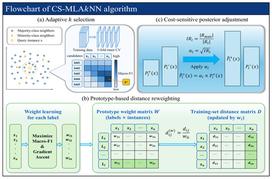
Figure 3. Flowchart of the proposed CS-MLAkNN algorithm.

The overall procedure of the proposed CS-MLAkNN algorithm is summarized in Algorithm 1. Generally, the execution flow is divided into four key phases. First, the algorithm initiates the data preparation and parameter selection phase. As outlined in Lines 2–3, the dataset is loaded, and features are standardized. Subsequently, Line 4 employs inner cross-validation to select the optimal neighbor count $k$. Second, the instance weighting phase is executed. In Line 6, specific weights for each instance are learned for every label. Following this, Lines 7–8 compute both the original Euclidean distance matrix and the weighted distance matrix, respectively. Third, during the training and prediction phase, Line 10 calculates the prior probabilities and conditional likelihoods. Line 11 then executes the posterior decision strategy, which amplifies the positive class probability to generate final label predictions. Finally, the performance evaluation phase is conducted. Line 13 computes various multi-label evaluation metrics. The algorithm concludes in Line 14 by returning both the predicted label matrix and the corresponding performance results. By integrating feature-level and label-level cost-sensitive mechanisms into the ML-kNN framework, this entire process significantly improves classification performance in the presence of class imbalance.

Algorithm 1: CS-MLAkNN

Input: Multi-label training set $D=\left\{\right(x_i,y_i){\}}_{i=1}^N$ Candidate neighbor set $\mathcal{K}$ Number of inner folds $F_{\mathrm{in}}$ Smoothing parameter $s$ Output: Y_pred—Predicted label matrix metrics—Performance metrics (F1 and G1 series)

Procedure:

// Data Preparation & Parameter Selection Stage 1.  $X, Y \leftarrow \mathrm{LoadDataset}(D$) // Load feature and label matrices 2.  $X_{std}$$\leftarrow \mathrm{Standardize}(X$)  // Standardize features (zero mean, unit variance) 3. $k^{\ast }$$\leftarrow \mathrm{InnerCV}\text{\_}\mathrm{Select}\text{\_}k(X_{std}$$, Y$)  // Select optimal k via inner cross-validation // Instance Weight Learning & Distance Weighting Stage 4.  $W \leftarrow \mathrm{FitLabelWeights}(X_{std}$$, Y$$, k^{\ast }$)  // Learn instance weights for each label 5.  $D_{train}$$\leftarrow \mathrm{PairwiseDistance}(X_{std}$)  // Compute pairwise Euclidean distance matrix 6.  $D_{\mathrm{w}\mathrm{e}\mathrm{i}\mathrm{g}\mathrm{h}\mathrm{t}\mathrm{e}\mathrm{d}}$$\leftarrow \mathrm{ApplyWeightsToDistances}(D_{train}$$, W$$, k^{\ast }$)  // Apply weights to distance matrix // Training & Prediction Stage 7.  $Ph, Peh$$\leftarrow \mathrm{ComputeML}k\mathrm{NNProbabilities}(Y$$, D_{train}$$, W$$, k^{\ast }$)  // Compute prior and likelihood probabilities 8.  $Y_{pred}$$\leftarrow \mathrm{PredictTestInstances}(X_{test}$$, X_{std}$$, Y$$, W$$, Ph$$, Peh$$, k^{\ast }$)  // Predict labels for test instances //Performance Evaluation Stage 9.  metrics$\leftarrow \mathrm{Evaluate}(Y_{true}$$, Y_{pred}$)  // Calculate multiple multi-label evaluation metrics 10. return $Y_{pred}$, metrics  // Return predictions and performance metrics

4. Experiments

This section systematically validates the effectiveness of the proposed CS-MLAkNN algorithm. Extensive experiments were conducted on 14 benchmark multi-label imbalanced datasets, covering comparative experiments, statistical analysis, ablation studies, and runtime analysis. Specifically, this study aims to address the following four research questions:

RQ1. 

Does CS-MLAkNN outperform state-of-the-art multi-label imbalanced learning methods across various scenarios?

RQ2. 

Does the algorithm demonstrate robustness across datasets with varying imbalance levels?

RQ3. 

What are the individual contributions of the cost-sensitive modeling and the adaptive neighbor mechanism to the overall performance?

RQ4. 

Does CS-MLAkNN maintain acceptable computational efficiency while achieving performance improvements?

4.1. Datasets

To comprehensively evaluate the performance of the proposed method, 14 benchmark multi-label datasets were selected from the MLC Toolbox [34]. These datasets include Emotions, Flags, Medical, Enron, Yeast, Scene, Genbase, Bio3, Image, Birds, Foodtruck, PlantPseAAC, CAL500, and Water-quality-nom. They encompass a wide range of application domains, such as music, image, text, and bioinformatics. Furthermore, these datasets exhibit significant diversity in terms of label count, feature dimensionality, and class imbalance level, thereby reflecting the complexity of real-world multi-label tasks. Table 2 summarizes several key statistical information for each dataset, including the number of instances (#Instance), features (#Feature), and labels (#Label).

Table 2. Details of the fourteen multi-label datasets used in the experiments.

Dataset	#Instance	#Feature	#Label	MeanIR	Field
emotions	593	72	6	2.320	Music
flags	194	19	7	1.859	Image
medical	978	1449	45	328.069	Text
enron	1702	1001	53	136.862	Text
yeast	2417	103	14	8.579	Text
scene	2407	294	6	4.662	Image
genbase	662	1188	27	143.458	Biology
bio3	310	1183	8	3.496	Biology
image	2000	294	5	3.116	Image
birds	645	260	19	32.859	Audio
foodtruck	407	743	12	8.788	Food
PlantPseAAC	978	687	12	21.879	Biology
CAL500	502	68	174	22.266	Music
water-quality-nom	1060	16	14	2.021	Chemistry

4.2. Experimental Settings

In this study, all experiments were conducted in a Python 3.12 environment with hardware configured as an Intel(R) Core(TM) Ultra 9 275HX-CPU and 32 GB RAM. The source code for our proposed CS-MLAkNN algorithm is publicly available at https://github.com/duanjicong1997/CS-MLAkNN/ (accessed on 17 August 2025).

To ensure the reproducibility of our experiments, the specific parameter settings for CS-MLAkNN are detailed as follows. The adaptive neighborhood size $k$ is dynamically selected from the integer search range [3, 20] based on local density estimation. In the prototype weighting formula, the smoothing parameter $\beta$ is set to 8.0 to control the influence of distance decay. For the feature-level cost optimization process, we employ a gradient descent strategy with a maximum of 100 iterations. To balance computational efficiency and convergence stability, an early stopping mechanism is introduced, where the optimization terminates if the loss reduction is less than the tolerance threshold of ${10}^{-6}$ for 6 consecutive epochs.

To validate the effectiveness and superiority of the proposed algorithm, CS-MLAkNN was compared with several state-of-the-art multi-label class imbalance learning methods, including BRWDkNN [24], MWBRWDNN [25], ML-ROS [8], ML-SMOTE [20], MLSOL [9], MLONC [10], DR-SMOTE [17], COCOA [14], LW-ELM [11], ML-KNN [15], ECC [13,32], and Rakel [31]. For fairness and objectivity, all comparison algorithms used the default parameter settings recommended in the corresponding references, with the base classifier uniformly set to ML-kNN (excluding algorithms that do not require a base classifier). For evaluation metrics, six common metrics were used to comprehensively assess the performance of the compared algorithms, including $F_{macro}$, $F_{micro}$, $F_{example}$, as well as $G_{macro}$, $G_{micro}$ and $G_{example}$, which are imbalance-sensitive metrics [35,36]. The definitions of these metrics are as follows:

$$F_{macro}={\displaystyle \frac{1}{L}}{\sum }_{l=1}^L{\displaystyle \frac{{2TP}_l}{{2TP}_l+{FP}_l+{FN}_l}}$$

(22)

$$F_{micro}={\displaystyle \frac{2TP}{2TP+FP+FN}}$$

(23)

$$F_{example}={\displaystyle \frac{1}{N}}{\sum }_{i=1}^N{\displaystyle \frac{{2TP}_i}{{2TP}_i+{FP}_i+{FN}_i}}$$

(24)

$$G_{macro}={\displaystyle \frac{1}{L}}{\sum }_{l=1}^L\sqrt{{\displaystyle \frac{{TP}_l\times {TN}_l}{\left({TP}_l+{FN}_l\right)\times \left({TN}_l+{FP}_l\right)}}}$$

(25)

$$G_{micro}=\sqrt{{\displaystyle \frac{TP\times TN}{\left(TP+FN\right)\times \left(TN+FP\right)}}}$$

(26)

$$G_{example}={\displaystyle \frac{1}{N}}{\sum }_{i=1}^N\sqrt{{\displaystyle \frac{{TP}_i\times {TN}_i}{\left({TP}_i+{FN}_i\right)\times \left({TN}_i+{FP}_i\right)}}}$$

(27)

The values of $TP$, $TN$, $FN$ and $FP$ can be obtained from the confusion matrix described in Table 3.

Table 3. Confusion matrix.

	Predicted Positive	Predicted Negative
Actual Positive	$TP$	$FN$
Actual Negative	$FP$	$TN$

Finally, considering the randomness of various learning algorithms, we performed 10 times’ random 5-fold cross-validation for each comparison algorithm and further presented the performance of each algorithm using the mean ± standard deviation [37].

4.3. Results and Discussions

Table 4, Table 5, Table 6, Table 7, Table 8 and Table 9 present the average performance of each comparison algorithm across six evaluation metrics on the 14 benchmark datasets, with the best results highlighted in bold. From these experimental results, the following conclusions can be drawn:

Table 4. $F_{macro}$ results of the comparative algorithms on fourteen multi-label datasets in where the best result on each dataset has been highlighted in bold.

Dataset	CS-MLAkNN	BRWDkNN	MWBRWDNN	ML-ROS	ML-SMOTE	MLSOL	MLONC	DR-SMOTE	COCOA	LW-ELM	ML-kNN	ECC	Rakel
emotions	0.6524 ± 0.0158	0.6088 ± 0.0110	0.6362 ± 0.0270	0.6328 ± 0.0219	0.6388 ± 0.0276	0.6255 ± 0.0297	0.6425 ± 0.0262	0.6364 ± 0.0245	0.6415 ± 0.0273	0.6297 ± 0.0191	0.6078 ± 0.0299	0.6417 ± 0.0218	0.6330 ± 0.0346
flags	0.6611 ± 0.0370	0.6608 ± 0.0305	0.6037 ± 0.0362	0.6145 ± 0.0327	0.6267 ± 0.0298	0.6124 ± 0.0362	0.6240 ± 0.0333	0.6048 ± 0.0407	0.6178 ± 0.0374	0.6430 ± 0.0494	0.5484 ± 0.0402	0.6061 ± 0.0338	0.5881 ± 0.0387
medical	0.1884 ± 0.0249	0.1625 ± 0.0156	0.1459 ± 0.0179	0.1724 ± 0.0186	0.1802 ± 0.0173	0.1992 ± 0.0249	0.1817 ± 0.0187	0.1740 ± 0.0145	0.1499 ± 0.0179	0.1649 ± 0.0107	0.2114 ± 0.0245	0.1473 ± 0.0162	0.1019 ± 0.0117
enron	0.1546 ± 0.0110	0.1509 ± 0.0069	0.0917 ± 0.0075	0.1250 ± 0.0218	0.1158 ± 0.0189	0.1113 ± 0.0120	0.1234 ± 0.0199	0.0939 ± 0.0074	0.0921 ± 0.0073	0.1252 ± 0.0067	0.0729 ± 0.0068	0.0924 ± 0.0070	0.0505 ± 0.0037
yeast	0.4783 ± 0.0070	0.4782 ± 0.0054	0.4257 ± 0.0155	0.4343 ± 0.0179	0.4307 ± 0.0125	0.4398 ± 0.0088	0.4405 ± 0.0098	0.4257 ± 0.0147	0.4319 ± 0.0143	0.4309 ± 0.0145	0.3654 ± 0.0081	0.4277 ± 0.0130	0.3825 ± 0.0129
scene	0.7289 ± 0.0138	0.6936 ± 0.0152	0.7184 ± 0.0200	0.7452 ± 0.0185	0.7362 ± 0.0242	0.7175 ± 0.0115	0.7461 ± 0.0173	0.7443 ± 0.0199	0.7219 ± 0.0215	0.6638 ± 0.0128	0.7379 ± 0.0233	0.7181 ± 0.0208	0.7304 ± 0.0215
genbase	0.6956 ± 0.0367	0.6366 ± 0.0372	0.6292 ± 0.0421	0.6909 ± 0.0540	0.6294 ± 0.0582	0.6270 ± 0.0562	0.6926 ± 0.0545	0.6227 ± 0.0450	0.6226 ± 0.0443	0.6359 ± 0.0190	0.6078 ± 0.0292	0.6206 ± 0.0432	0.6154 ± 0.0444
bio3	0.4714 ± 0.0205	0.4851 ± 0.0192	0.4495 ± 0.0221	0.4729 ± 0.0202	0.4647 ± 0.0131	0.4754 ± 0.0184	0.4880 ± 0.0149	0.4593 ± 0.0185	0.4724 ± 0.0106	0.4611 ± 0.0294	0.3030 ± 0.0223	0.4603 ± 0.0209	0.4524 ± 0.0267
image	0.6136 ± 0.0137	0.5768 ± 0.0125	0.5905 ± 0.0150	0.5963 ± 0.0132	0.5894 ± 0.0127	0.5890 ± 0.0123	0.6002 ± 0.0149	0.5998 ± 0.0156	0.5891 ± 0.0186	0.5978 ± 0.0130	0.5777 ± 0.0191	0.5749 ± 0.0171	0.5927 ± 0.0155
birds	0.2849 ± 0.0286	0.2551 ± 0.0306	0.1656 ± 0.0263	0.2505 ± 0.0388	0.2369 ± 0.0611	0.2639 ± 0.0234	0.2542 ± 0.0573	0.2171 ± 0.0284	0.1592 ± 0.0395	0.2483 ± 0.0245	0.1485 ± 0.0250	0.1643 ± 0.0395	0.1725 ± 0.0389
foodtruck	0.2502 ± 0.0244	0.2943 ± 0.0192	0.1719 ± 0.0259	0.2071 ± 0.0262	0.1955 ± 0.0253	0.2269 ± 0.0339	0.1975 ± 0.0179	0.1739 ± 0.0189	0.1779 ± 0.0213	0.2410 ± 0.0236	0.1040 ± 0.0171	0.1613 ± 0.0163	0.1596 ± 0.0177
PlantPseAAC	0.1613 ± 0.0205	0.1696 ± 0.0152	0.0979 ± 0.0194	0.1489 ± 0.0263	0.1275 ± 0.0208	0.1399 ± 0.0342	0.1406 ± 0.0243	0.1260 ± 0.0221	0.0999 ± 0.0195	0.1464 ± 0.0253	0.0812 ± 0.0217	0.0923 ± 0.0163	0.0937 ± 0.0214
CAL500	0.1893 ± 0.0051	0.2263 ± 0.0031	0.1150 ± 0.0093	0.1196 ± 0.0111	0.1096 ± 0.0077	0.1294 ± 0.0094	0.1267 ± 0.0088	0.1131 ± 0.0092	0.1195 ± 0.0079	0.1614 ± 0.0078	0.0508 ± 0.0057	0.1193 ± 0.0103	0.0244 ± 0.0023
water-quality-nom	0.5815 ± 0.0119	0.5538 ± 0.0122	0.5047 ± 0.0128	0.5093 ± 0.0116	0.5043 ± 0.0092	0.5101 ± 0.0093	0.5116 ± 0.0134	0.5035 ± 0.0117	0.5196 ± 0.0107	0.5017 ± 0.0159	0.3972 ± 0.0251	0.5101 ± 0.0090	0.4485 ± 0.0100

Table 5. $F_{micro}$ results of the comparative algorithms on fourteen multi-label datasets in where the best result on each dataset has been highlighted in bold.

Dataset	CS-MLAkNN	BRWDkNN	MWBRWDNN	ML-ROS	ML-SMOTE	MLSOL	MLONC	DR-SMOTE	COCOA	LW-ELM	ML-kNN	ECC	Rakel
emotions	0.6526 ± 0.0191	0.5944 ± 0.0110	0.6533 ± 0.0279	0.6486 ± 0.0238	0.6549 ± 0.0308	0.6403 ± 0.0288	0.6574 ± 0.0277	0.6537 ± 0.0272	0.6565 ± 0.0297	0.6320 ± 0.0192	0.6413 ± 0.0331	0.6600 ± 0.0228	0.6524 ± 0.0344
flags	0.7197 ± 0.0257	0.7186 ± 0.0326	0.7044 ± 0.0301	0.6948 ± 0.0312	0.7053 ± 0.0308	0.7020 ± 0.0305	0.7017 ± 0.0334	0.7029 ± 0.0355	0.7133 ± 0.0336	0.6787 ± 0.0478	0.7097 ± 0.0331	0.7020 ± 0.0312	0.6889 ± 0.0364
medical	0.4269 ± 0.0242	0.2938 ± 0.0142	0.5009 ± 0.0219	0.4687 ± 0.0203	0.5007 ± 0.0289	0.1992 ± 0.0249	0.4700 ± 0.0184	0.5374 ± 0.0178	0.5040 ± 0.0172	0.3049 ± 0.0161	0.5416 ± 0.0339	0.4687 ± 0.0189	0.4305 ± 0.0217
enron	0.4828 ± 0.0125	0.2991 ± 0.0086	0.3175 ± 0.0162	0.3321 ± 0.0161	0.3417 ± 0.0265	0.3334 ± 0.0164	0.3276 ± 0.0151	0.3295 ± 0.0151	0.3222 ± 0.0147	0.4656 ± 0.0196	0.4115 ± 0.0175	0.3192 ± 0.0147	0.2314 ± 0.0051
yeast	0.6374 ± 0.0067	0.6338 ± 0.0059	0.6374 ± 0.0135	0.6254 ± 0.0147	0.6135 ± 0.0156	0.6227 ± 0.0092	0.6264 ± 0.0114	0.6372 ± 0.0123	0.6407 ± 0.0112	0.5926 ± 0.0096	0.6396 ± 0.0129	0.6389 ± 0.0110	0.6026 ± 0.0123
scene	0.7148 ± 0.0155	0.6170 ± 0.0108	0.7136 ± 0.0193	0.7366 ± 0.0181	0.7303 ± 0.0237	0.7079 ± 0.0126	0.7379 ± 0.0174	0.7361 ± 0.0194	0.7150 ± 0.0215	0.6607 ± 0.0140	0.7237 ± 0.0236	0.7108 ± 0.0192	0.7214 ± 0.0198
genbase	0.9333 ± 0.0304	0.9542 ± 0.0175	0.9538 ± 0.0191	0.9633 ± 0.0192	0.9373 ± 0.0309	0.9517 ± 0.0199	0.9597 ± 0.0186	0.9529 ± 0.0190	0.9540 ± 0.0169	0.8967 ± 0.0320	0.9502 ± 0.0156	0.9479 ± 0.0207	0.9469 ± 0.0198
bio3	0.5736 ± 0.0201	0.5504 ± 0.0237	0.5762 ± 0.0166	0.5785 ± 0.0141	0.5756 ± 0.0165	0.5744 ± 0.0155	0.5827 ± 0.0148	0.5853 ± 0.0161	0.5892 ± 0.0136	0.5233 ± 0.0324	0.5668 ± 0.0200	0.5840 ± 0.0163	0.5700 ± 0.0195
image	0.6076 ± 0.0163	0.5466 ± 0.0115	0.5929 ± 0.0162	0.5963 ± 0.0140	0.5890 ± 0.0136	0.5888 ± 0.0128	0.5999 ± 0.0155	0.5999 ± 0.0161	0.5918 ± 0.0195	0.5962 ± 0.0119	0.5694 ± 0.0189	0.5775 ± 0.0182	0.5953 ± 0.0154
birds	0.3525 ± 0.0257	0.2829 ± 0.0311	0.2779 ± 0.0341	0.2975 ± 0.0314	0.2801 ± 0.0359	0.3211 ± 0.0306	0.2933 ± 0.0379	0.2878 ± 0.0236	0.2659 ± 0.0421	0.3124 ± 0.0211	0.2160 ± 0.0282	0.1837 ± 0.0309	0.1759 ± 0.0382
foodtruck	0.4852 ± 0.0181	0.3759 ± 0.0169	0.4908 ± 0.0260	0.4784 ± 0.0237	0.5031 ± 0.0303	0.4878 ± 0.0201	0.4863 ± 0.0220	0.5060 ± 0.0255	0.5035 ± 0.0267	0.4425 ± 0.0204	0.4589 ± 0.0298	0.4980 ± 0.0204	0.4907 ± 0.0289
PlantPseAAC	0.3276 ± 0.0199	0.2328 ± 0.0106	0.2272 ± 0.0364	0.2737 ± 0.0384	0.2036 ± 0.0359	0.2480 ± 0.0506	0.1961 ± 0.0264	0.2780 ± 0.0355	0.2290 ± 0.0403	0.2627 ± 0.0287	0.2636 ± 0.0362	0.2025 ± 0.0294	0.2114 ± 0.0300
CAL500	0.4476 ± 0.0112	0.3561 ± 0.0077	0.3619 ± 0.0126	0.3584 ± 0.0091	0.3636 ± 0.0162	0.3680 ± 0.0148	0.3736 ± 0.0112	0.3620 ± 0.0117	0.3715 ± 0.0109	0.3702 ± 0.0129	0.3214 ± 0.0072	0.3717 ± 0.0157	0.1363 ± 0.0045
water-quality-nom	0.6052 ± 0.0102	0.5916 ± 0.0110	0.5569 ± 0.0101	0.5570 ± 0.0121	0.5582 ± 0.0076	0.5568 ± 0.0079	0.5598 ± 0.0125	0.5560 ± 0.0117	0.5690 ± 0.0109	0.5467 ± 0.0151	0.5199 ± 0.0184	0.5654 ± 0.0076	0.5249 ± 0.0090

Table 6. $F_{example}$ results of the comparative algorithms on fourteen multi-label datasets in where the best result on each dataset has been highlighted in bold.

Dataset	CS-MLAkNN	BRWDkNN	MWBRWDNN	ML-ROS	ML-SMOTE	MLSOL	MLONC	DR-SMOTE	COCOA	LW-ELM	ML-kNN	ECC	Rakel
emotions	0.6495 ± 0.0190	0.5943 ± 0.0122	0.6109 ± 0.0325	0.6166 ± 0.0297	0.6198 ± 0.0325	0.6124 ± 0.0319	0.6224 ± 0.0312	0.6205 ± 0.0302	0.6235 ± 0.0314	0.6065 ± 0.0229	0.6071 ± 0.0350	0.6273 ± 0.0257	0.6232 ± 0.0345
flags	0.7013 ± 0.0265	0.6989 ± 0.0393	0.6703 ± 0.0388	0.6581 ± 0.0384	0.6722 ± 0.0385	0.6674 ± 0.0370	0.6684 ± 0.0395	0.6688 ± 0.0421	0.6836 ± 0.0388	0.6077 ± 0.0645	0.6902 ± 0.0325	0.6699 ± 0.0360	0.6572 ± 0.0406
medical	0.4350 ± 0.0338	0.3504 ± 0.0223	0.4110 ± 0.0187	0.4620 ± 0.0183	0.4963 ± 0.0277	0.1992 ± 0.0249	0.4622 ± 0.0170	0.5310 ± 0.0212	0.4164 ± 0.0198	0.3496 ± 0.0187	0.5357 ± 0.0378	0.4563 ± 0.0198	0.4133 ± 0.0245
enron	0.4805 ± 0.0139	0.3465 ± 0.0070	0.2739 ± 0.0180	0.3202 ± 0.0195	0.3304 ± 0.0237	0.3142 ± 0.0168	0.3178 ± 0.0208	0.3199 ± 0.0206	0.2833 ± 0.0198	0.4456 ± 0.0223	0.3635 ± 0.0153	0.3078 ± 0.0220	0.2427 ± 0.0104
yeast	0.6370 ± 0.0084	0.6337 ± 0.0069	0.6086 ± 0.0144	0.5985 ± 0.0144	0.5866 ± 0.0169	0.5977 ± 0.0097	0.6062 ± 0.0105	0.6092 ± 0.0118	0.6159 ± 0.0105	0.5703 ± 0.0100	0.6119 ± 0.0132	0.6119 ± 0.0113	0.5780 ± 0.0121
scene	0.7462 ± 0.0143	0.6392 ± 0.0122	0.6801 ± 0.0178	0.7407 ± 0.0184	0.7347 ± 0.0242	0.7118 ± 0.0131	0.7418 ± 0.0185	0.7399 ± 0.0200	0.6923 ± 0.0205	0.6773 ± 0.0182	0.7274 ± 0.0250	0.7144 ± 0.0198	0.7253 ± 0.0201
genbase	0.9558 ± 0.0191	0.9573 ± 0.0195	0.9546 ± 0.0217	0.9697 ± 0.0183	0.9565 ± 0.0236	0.9631 ± 0.0198	0.9678 ± 0.0176	0.9638 ± 0.0186	0.9570 ± 0.0203	0.9422 ± 0.0182	0.9605 ± 0.0158	0.9578 ± 0.0200	0.9574 ± 0.0202
bio3	0.5567 ± 0.0199	0.5308 ± 0.0212	0.5406 ± 0.0159	0.5456 ± 0.0126	0.5461 ± 0.0182	0.5402 ± 0.0191	0.5500 ± 0.0185	0.5552 ± 0.0171	0.5566 ± 0.0122	0.4662 ± 0.0357	0.5416 ± 0.0247	0.5531 ± 0.0162	0.5378 ± 0.0175
image	0.6320 ± 0.0178	0.5657 ± 0.0138	0.5599 ± 0.0205	0.6031 ± 0.0158	0.5958 ± 0.0155	0.5945 ± 0.0155	0.6073 ± 0.0170	0.6078 ± 0.0174	0.5754 ± 0.0216	0.5973 ± 0.0135	0.5736 ± 0.0191	0.5860 ± 0.0199	0.6041 ± 0.0162
birds	0.5357 ± 0.0275	0.5205 ± 0.0266	0.5429 ± 0.0367	0.1957 ± 0.0260	0.1865 ± 0.0251	0.2089 ± 0.0287	0.1947 ± 0.0303	0.1967 ± 0.0271	0.5349 ± 0.0402	0.5200 ± 0.0323	0.1406 ± 0.0250	0.1120 ± 0.0233	0.1037 ± 0.0246
foodtruck	0.4746 ± 0.0259	0.3638 ± 0.0179	0.4818 ± 0.0324	0.4864 ± 0.0246	0.5025 ± 0.0324	0.4818 ± 0.0250	0.4874 ± 0.0284	0.5130 ± 0.0277	0.4974 ± 0.0316	0.4218 ± 0.0308	0.5024 ± 0.0322	0.5049 ± 0.0242	0.5027 ± 0.0300
PlantPseAAC	0.3092 ± 0.0237	0.2439 ± 0.0117	0.1644 ± 0.0284	0.2716 ± 0.0380	0.2008 ± 0.0367	0.2472 ± 0.0518	0.1930 ± 0.0272	0.2759 ± 0.0363	0.1708 ± 0.0314	0.2103 ± 0.0268	0.2667 ± 0.0353	0.2006 ± 0.0295	0.2103 ± 0.0307
CAL500	0.4452 ± 0.0108	0.3571 ± 0.0074	0.3567 ± 0.0114	0.3539 ± 0.0087	0.3588 ± 0.0153	0.3617 ± 0.0147	0.3661 ± 0.0114	0.3572 ± 0.0113	0.3671 ± 0.0109	0.3652 ± 0.0117	0.3254 ± 0.0070	0.3670 ± 0.0140	0.1372 ± 0.0050
water-quality-nom	0.5815 ± 0.0091	0.5636 ± 0.0118	0.5274 ± 0.0125	0.5283 ± 0.0131	0.5308 ± 0.0092	0.5278 ± 0.0088	0.5284 ± 0.0135	0.5266 ± 0.0135	0.5409 ± 0.0122	0.5011 ± 0.0173	0.4961 ± 0.0211	0.5350 ± 0.0109	0.4977 ± 0.0119

Table 7. $G_{macro}$ results of the comparative algorithms on fourteen multi-label datasets in where the best result on each dataset has been highlighted in bold.

Dataset	CS-MLAkNN	BRWDkNN	MWBRWDNN	ML-ROS	ML-SMOTE	MLSOL	MLONC	DR-SMOTE	COCOA	LW-ELM	ML-kNN	ECC	Rakel
emotions	0.7365 ± 0.0168	0.6640 ± 0.0077	0.6444 ± 0.0267	0.6391 ± 0.0215	0.6445 ± 0.0282	0.6319 ± 0.0299	0.6486 ± 0.0264	0.6437 ± 0.0250	0.6484 ± 0.0278	0.7325 ± 0.0179	0.6305 ± 0.0321	0.6483 ± 0.0216	0.6404 ± 0.0335
flags	0.3978 ± 0.0437	0.6902 ± 0.0259	0.6279 ± 0.0404	0.6344 ± 0.0325	0.6477 ± 0.0288	0.6267 ± 0.0414	0.6358 ± 0.0349	0.6300 ± 0.0373	0.6429 ± 0.0322	0.6386 ± 0.0388	0.5755 ± 0.0573	0.6301 ± 0.0319	0.6147 ± 0.0384
medical	0.6081 ± 0.0431	0.2055 ± 0.0193	0.1675 ± 0.0177	0.1959 ± 0.0232	0.2047 ± 0.0173	0.1992 ± 0.0249	0.2052 ± 0.0211	0.1985 ± 0.0155	0.1706 ± 0.0188	0.7790 ± 0.0481	0.2269 ± 0.0239	0.1742 ± 0.0169	0.1209 ± 0.0152
enron	0.3239 ± 0.0367	0.2327 ± 0.0090	0.1177 ± 0.0091	0.1515 ± 0.0250	0.1437 ± 0.0230	0.1353 ± 0.0144	0.1555 ± 0.0249	0.1207 ± 0.0078	0.1182 ± 0.0083	0.2653 ± 0.0234	0.0897 ± 0.0108	0.1209 ± 0.0071	0.0688 ± 0.0054
yeast	0.4706 ± 0.0168	0.4907 ± 0.0053	0.4577 ± 0.0230	0.4486 ± 0.0222	0.4558 ± 0.0164	0.4470 ± 0.0088	0.4568 ± 0.0122	0.4580 ± 0.0238	0.4619 ± 0.0235	0.5075 ± 0.0227	0.4228 ± 0.0146	0.4590 ± 0.0226	0.4073 ± 0.0195
scene	0.8707 ± 0.0080	0.7476 ± 0.0116	0.7363 ± 0.0198	0.7532 ± 0.0195	0.7484 ± 0.0223	0.7274 ± 0.0119	0.7543 ± 0.0178	0.7537 ± 0.0200	0.7378 ± 0.0208	0.8394 ± 0.0091	0.7431 ± 0.0209	0.7302 ± 0.0196	0.7433 ± 0.0209
genbase	0.9649 ± 0.0303	0.6433 ± 0.0362	0.6362 ± 0.0409	0.6964 ± 0.0538	0.6366 ± 0.0574	0.6342 ± 0.0560	0.6984 ± 0.0545	0.6292 ± 0.0449	0.6292 ± 0.0443	0.9645 ± 0.0286	0.6131 ± 0.0291	0.6276 ± 0.0433	0.6217 ± 0.0448
bio3	0.3844 ± 0.0339	0.5445 ± 0.0133	0.4650 ± 0.0235	0.4822 ± 0.0210	0.4801 ± 0.0145	0.4821 ± 0.0191	0.4977 ± 0.0143	0.4733 ± 0.0210	0.4845 ± 0.0143	0.5801 ± 0.0269	0.3691 ± 0.0258	0.4745 ± 0.0217	0.4631 ± 0.0289
image	0.7501 ± 0.0155	0.6330 ± 0.0123	0.6053 ± 0.0167	0.6097 ± 0.0132	0.6051 ± 0.0122	0.6006 ± 0.0138	0.6148 ± 0.0149	0.6137 ± 0.0160	0.6056 ± 0.0194	0.7367 ± 0.0090	0.5981 ± 0.0203	0.6005 ± 0.0176	0.6071 ± 0.0158
birds	0.5758 ± 0.0765	0.3498 ± 0.0395	0.1968 ± 0.0250	0.2899 ± 0.0422	0.2814 ± 0.0641	0.2901 ± 0.0233	0.2923 ± 0.0656	0.2548 ± 0.0370	0.1937 ± 0.0412	0.5691 ± 0.0552	0.1870 ± 0.0247	0.2348 ± 0.0446	0.2402 ± 0.0475
foodtruck	0.3070 ± 0.0643	0.3953 ± 0.0240	0.1925 ± 0.0375	0.2295 ± 0.0361	0.2288 ± 0.0304	0.2437 ± 0.0390	0.2215 ± 0.0242	0.1968 ± 0.0288	0.2026 ± 0.0324	0.3477 ± 0.0513	0.1439 ± 0.0247	0.1814 ± 0.0232	0.1822 ± 0.0263
PlantPseAAC	0.3046 ± 0.0692	0.2577 ± 0.0216	0.1194 ± 0.0255	0.1719 ± 0.0318	0.1633 ± 0.0216	0.1738 ± 0.0370	0.1838 ± 0.0352	0.1528 ± 0.0256	0.1300 ± 0.0200	0.2756 ± 0.0389	0.1083 ± 0.0300	0.1445 ± 0.0206	0.1425 ± 0.0341
CAL500	0.2159 ± 0.0130	0.3106 ± 0.0055	0.1268 ± 0.0105	0.1315 ± 0.0126	0.1229 ± 0.0095	0.1405 ± 0.0114	0.1386 ± 0.0103	0.1261 ± 0.0105	0.1309 ± 0.0084	0.2742 ± 0.0167	0.0596 ± 0.0072	0.1322 ± 0.0113	0.0264 ± 0.0024
water-quality-nom	0.6039 ± 0.0131	0.5576 ± 0.0120	0.5140 ± 0.0133	0.5159 ± 0.0123	0.5149 ± 0.0093	0.5159 ± 0.0096	0.5181 ± 0.0141	0.5134 ± 0.0128	0.5271 ± 0.0118	0.5909 ± 0.0138	0.4518 ± 0.0297	0.5217 ± 0.0099	0.4596 ± 0.0096

Table 8. $G_{micro}$ results of the comparative algorithms on fourteen multi-label datasets in where the best result on each dataset has been highlighted in bold.

Dataset	CS-MLAkNN	BRWDkNN	MWBRWDNN	ML-ROS	ML-SMOTE	MLSOL	MLONC	DR-SMOTE	COCOA	LW-ELM	ML-kNN	ECC	Rakel
emotions	0.7491 ± 0.0174	0.6394 ± 0.0084	0.6540 ± 0.0279	0.6489 ± 0.0238	0.6552 ± 0.0308	0.6405 ± 0.0289	0.6577 ± 0.0279	0.6542 ± 0.0273	0.6567 ± 0.0297	0.7335 ± 0.0165	0.6438 ± 0.0331	0.6603 ± 0.0229	0.6527 ± 0.0346
flags	0.6180 ± 0.0259	0.7345 ± 0.0302	0.7047 ± 0.0302	0.6950 ± 0.0312	0.7054 ± 0.0309	0.7021 ± 0.0305	0.7019 ± 0.0333	0.7032 ± 0.0356	0.7138 ± 0.0334	0.6886 ± 0.0355	0.7105 ± 0.0331	0.7023 ± 0.0312	0.6898 ± 0.0366
medical	0.7164 ± 0.0263	0.3610 ± 0.0141	0.5171 ± 0.0239	0.4693 ± 0.0202	0.5016 ± 0.0294	0.1992 ± 0.0249	0.4705 ± 0.0183	0.5383 ± 0.0183	0.5186 ± 0.0209	0.8075 ± 0.0208	0.5429 ± 0.0337	0.4694 ± 0.0190	0.4312 ± 0.0219
enron	0.7529 ± 0.0157	0.3784 ± 0.0072	0.3542 ± 0.0154	0.3533 ± 0.0158	0.3659 ± 0.0261	0.3498 ± 0.0157	0.3511 ± 0.0152	0.3539 ± 0.0149	0.3579 ± 0.0137	0.6438 ± 0.0156	0.4357 ± 0.0169	0.3421 ± 0.0154	0.2589 ± 0.0051
yeast	0.7432 ± 0.0069	0.6446 ± 0.0051	0.6385 ± 0.0136	0.6260 ± 0.0148	0.6141 ± 0.0158	0.6231 ± 0.0093	0.6264 ± 0.0114	0.6383 ± 0.0124	0.6412 ± 0.0112	0.6988 ± 0.0091	0.6439 ± 0.0124	0.6398 ± 0.0111	0.6055 ± 0.0125
scene	0.8685 ± 0.0083	0.6402 ± 0.0104	0.7161 ± 0.0194	0.7368 ± 0.0181	0.7305 ± 0.0237	0.7080 ± 0.0126	0.7381 ± 0.0174	0.7364 ± 0.0194	0.7165 ± 0.0216	0.8360 ± 0.0102	0.7239 ± 0.0236	0.7111 ± 0.0192	0.7217 ± 0.0198
genbase	0.9864 ± 0.0079	0.9544 ± 0.0174	0.9542 ± 0.0190	0.9633 ± 0.0192	0.9376 ± 0.0309	0.9519 ± 0.0199	0.9598 ± 0.0185	0.9532 ± 0.0189	0.9545 ± 0.0166	0.9720 ± 0.0045	0.9504 ± 0.0155	0.9482 ± 0.0206	0.9472 ± 0.0197
bio3	0.6463 ± 0.0251	0.5954 ± 0.0171	0.5766 ± 0.0167	0.5810 ± 0.0132	0.5790 ± 0.0162	0.5765 ± 0.0160	0.5863 ± 0.0144	0.5865 ± 0.0159	0.5927 ± 0.0125	0.6386 ± 0.0246	0.5680 ± 0.0193	0.5851 ± 0.0162	0.5705 ± 0.0193
image	0.7581 ± 0.0111	0.5806 ± 0.0106	0.5993 ± 0.0158	0.5976 ± 0.0141	0.5904 ± 0.0136	0.5896 ± 0.0128	0.6014 ± 0.0155	0.6014 ± 0.0162	0.5954 ± 0.0197	0.7344 ± 0.0086	0.5713 ± 0.0189	0.5790 ± 0.0183	0.5969 ± 0.0154
birds	0.6914 ± 0.0473	0.3319 ± 0.0273	0.3222 ± 0.0320	0.2986 ± 0.0309	0.2807 ± 0.0360	0.3225 ± 0.0304	0.2942 ± 0.0377	0.2884 ± 0.0234	0.3260 ± 0.0392	0.6643 ± 0.0261	0.2164 ± 0.0283	0.1840 ± 0.0309	0.1762 ± 0.0381
foodtruck	0.6952 ± 0.0129	0.4620 ± 0.0116	0.4989 ± 0.0252	0.4804 ± 0.0243	0.5073 ± 0.0303	0.4890 ± 0.0203	0.4893 ± 0.0210	0.5134 ± 0.0241	0.5100 ± 0.0248	0.6270 ± 0.0224	0.4860 ± 0.0274	0.5059 ± 0.0194	0.5017 ± 0.0279
PlantPseAAC	0.6755 ± 0.0290	0.3429 ± 0.0097	0.2494 ± 0.0390	0.2738 ± 0.0384	0.2038 ± 0.0360	0.2481 ± 0.0506	0.1963 ± 0.0264	0.2782 ± 0.0355	0.2473 ± 0.0446	0.4697 ± 0.0298	0.2638 ± 0.0362	0.2026 ± 0.0294	0.2116 ± 0.0300
CAL500	0.7156 ± 0.0091	0.4495 ± 0.0058	0.3734 ± 0.0119	0.3672 ± 0.0084	0.3775 ± 0.0155	0.3746 ± 0.0143	0.3810 ± 0.0102	0.3739 ± 0.0110	0.3801 ± 0.0105	0.5631 ± 0.0126	0.3645 ± 0.0066	0.3817 ± 0.0147	0.2119 ± 0.0067
water-quality-nom	0.6408 ± 0.0106	0.5929 ± 0.0111	0.5582 ± 0.0099	0.5577 ± 0.0121	0.5595 ± 0.0076	0.5573 ± 0.0078	0.5605 ± 0.0122	0.5575 ± 0.0115	0.5691 ± 0.0109	0.6380 ± 0.0120	0.5285 ± 0.0155	0.5668 ± 0.0076	0.5287 ± 0.0086

Table 9. $G_{example}$ results of the comparative algorithms on fourteen multi-label datasets in where the best result on each dataset has been highlighted in bold.

Dataset	CS-MLAkNN	BRWDkNN	MWBRWDNN	ML-ROS	ML-SMOTE	MLSOL	MLONC	DR-SMOTE	COCOA	LW-ELM	ML-kNN	ECC	Rakel
emotions	0.7107 ± 0.0237	0.6443 ± 0.0099	0.6254 ± 0.0323	0.6311 ± 0.0295	0.6351 ± 0.0318	0.6273 ± 0.0314	0.6375 ± 0.0311	0.6354 ± 0.0297	0.6375 ± 0.0310	0.6871 ± 0.0274	0.6239 ± 0.0342	0.6418 ± 0.0255	0.6379 ± 0.0339
flags	0.5386 ± 0.0482	0.7213 ± 0.0378	0.6777 ± 0.0393	0.6648 ± 0.0386	0.6799 ± 0.0390	0.6751 ± 0.0373	0.6758 ± 0.0396	0.6760 ± 0.0428	0.6912 ± 0.0386	0.5501 ± 0.0545	0.6980 ± 0.0326	0.6769 ± 0.0366	0.6649 ± 0.0414
medical	0.5608 ± 0.0424	0.4067 ± 0.0213	0.4170 ± 0.0190	0.4685 ± 0.0193	0.5035 ± 0.0279	0.1992 ± 0.0249	0.4686 ± 0.0181	0.5384 ± 0.0208	0.4225 ± 0.0201	0.7106 ± 0.0341	0.5443 ± 0.0378	0.4628 ± 0.0200	0.4197 ± 0.0246
enron	0.7004 ± 0.0193	0.4177 ± 0.0058	0.2903 ± 0.0183	0.3397 ± 0.0185	0.3543 ± 0.0234	0.3322 ± 0.0166	0.3382 ± 0.0203	0.3405 ± 0.0197	0.3003 ± 0.0197	0.5667 ± 0.0205	0.3947 ± 0.0156	0.3262 ± 0.0216	0.2605 ± 0.0103
yeast	0.7272 ± 0.0076	0.6551 ± 0.0061	0.6227 ± 0.0139	0.6129 ± 0.0142	0.6004 ± 0.0168	0.6120 ± 0.0094	0.6201 ± 0.0099	0.6238 ± 0.0111	0.6290 ± 0.0100	0.6591 ± 0.0080	0.6296 ± 0.0126	0.6261 ± 0.0106	0.5938 ± 0.0119
scene	0.8297 ± 0.0120	0.6669 ± 0.0127	0.6827 ± 0.0175	0.7437 ± 0.0180	0.7377 ± 0.0239	0.7150 ± 0.0128	0.7448 ± 0.0182	0.7430 ± 0.0196	0.6951 ± 0.0203	0.7793 ± 0.0193	0.7310 ± 0.0247	0.7173 ± 0.0195	0.7282 ± 0.0197
genbase	0.9813 ± 0.0119	0.9592 ± 0.0191	0.9564 ± 0.0213	0.9708 ± 0.0181	0.9579 ± 0.0235	0.9650 ± 0.0195	0.9693 ± 0.0175	0.9658 ± 0.0184	0.9590 ± 0.0200	0.9751 ± 0.0054	0.9623 ± 0.0158	0.9597 ± 0.0195	0.9594 ± 0.0199
bio3	0.6110 ± 0.0313	0.5889 ± 0.0162	0.5615 ± 0.0169	0.5681 ± 0.0128	0.5689 ± 0.0178	0.5621 ± 0.0195	0.5737 ± 0.0193	0.5768 ± 0.0181	0.5802 ± 0.0118	0.5209 ± 0.0368	0.5623 ± 0.0238	0.5748 ± 0.0169	0.5590 ± 0.0172
image	0.7065 ± 0.0166	0.6059 ± 0.0131	0.5665 ± 0.0205	0.6107 ± 0.0159	0.6032 ± 0.0154	0.6023 ± 0.0155	0.6145 ± 0.0169	0.6152 ± 0.0173	0.5825 ± 0.0214	0.6612 ± 0.0145	0.5811 ± 0.0190	0.5929 ± 0.0198	0.6113 ± 0.0160
birds	0.7376 ± 0.0430	0.5461 ± 0.0237	0.5477 ± 0.0363	0.2036 ± 0.0267	0.1944 ± 0.0259	0.2172 ± 0.0294	0.2029 ± 0.0307	0.2055 ± 0.0281	0.5389 ± 0.0402	0.7116 ± 0.0386	0.1484 ± 0.0262	0.1171 ± 0.0244	0.1081 ± 0.0257
foodtruck	0.6721 ± 0.0199	0.4537 ± 0.0136	0.5095 ± 0.0353	0.5163 ± 0.0252	0.5308 ± 0.0350	0.5112 ± 0.0282	0.5149 ± 0.0289	0.5420 ± 0.0303	0.5256 ± 0.0346	0.5583 ± 0.0397	0.5353 ± 0.0321	0.5341 ± 0.0264	0.5329 ± 0.0321
PlantPseAAC	0.5142 ± 0.0461	0.3509 ± 0.0105	0.1656 ± 0.0284	0.2735 ± 0.0383	0.2022 ± 0.0370	0.2487 ± 0.0518	0.1947 ± 0.0271	0.2776 ± 0.0364	0.1719 ± 0.0315	0.2385 ± 0.0301	0.2676 ± 0.0357	0.2018 ± 0.0296	0.2115 ± 0.0308
CAL500	0.7141 ± 0.0095	0.4499 ± 0.0058	0.3724 ± 0.0108	0.3674 ± 0.0078	0.3766 ± 0.0146	0.3735 ± 0.0144	0.3799 ± 0.0109	0.3730 ± 0.0105	0.3794 ± 0.0106	0.5542 ± 0.0115	0.3684 ± 0.0066	0.3812 ± 0.0128	0.2138 ± 0.0074
water-quality-nom	0.5954 ± 0.0134	0.5820 ± 0.0116	0.5444 ± 0.0123	0.5453 ± 0.0126	0.5478 ± 0.0081	0.5446 ± 0.0091	0.5460 ± 0.0128	0.5437 ± 0.0126	0.5563 ± 0.0122	0.5757 ± 0.0205	0.5180 ± 0.0189	0.5529 ± 0.0114	0.5174 ± 0.0123

(1)

Overall, CS-MLAkNN demonstrates the most robust and superior performance across all six evaluation metrics. Specifically, on the 14 datasets, the proposed method achieved the best results 8, 7, 10, 8, 12, and 12 times, respectively, for each metric. In total, it secured 57 best results. This accounts for approximately two-thirds of the total 84 experimental cases (14 datasets $\times$ 6 metrics). Consequently, CS-MLAkNN significantly outperforms other comparison algorithms. For instance, the second-best method, BRWDkNN, obtained only 8 best results. It is worth noting that for the $G_{micro}$ and $G_{example}$ metrics, which emphasize the recall of minority classes, CS-MLAkNN achieved optimal or near-optimal performance on the majority of datasets. These results validate the effectiveness of the integrated feature-level and label-level cost-sensitive strategies, along with the adaptive $k$-value mechanism, in alleviating multi-label class imbalance.

(2)

Compared to other ML-CIL strategies, cost-sensitive methods based on k-nearest neighbors and ELM are relatively more competitive. Specifically, BRWDkNN and MWBRWDNN achieved high rankings on the $F_{macro}$ and $G_{macro}$ metrics for certain datasets, such as Flags, PlantPseAAC, and CAL500. This demonstrates their effectiveness on macro-average metrics. Similarly, LW-ELM obtained the highest $G_{macro}$ and $G_{micro}$ values on extremely imbalanced datasets like Medical. This result suggests that assigning different cost weights to labels can effectively improve the recognition capability for minority labels. However, the performance of these methods fluctuates significantly across different datasets. Their advantages diminish on moderately imbalanced or label-scarce datasets. In some cases, performance degradation is even observed in terms of $G-mean$ metrics. This phenomenon can be attributed to their inherent design limitations. BRWDkNN, MWBRWDNN, and LW-ELM typically apply cost-sensitive strategies only at the feature level or the label level, rather than both. Consequently, they fail to adapt effectively when the local neighborhood structure or label distribution undergoes significant changes. Therefore, although these methods remain competitive in specific scenarios, their overall average ranking is inferior to the CS-MLAkNN proposed in this paper.

(3)

It is also worth noting that the performance improvement of CS-MLAkNN varies across datasets depending on their imbalance characteristics. For datasets with relatively low imbalance ratios and small sample sizes, such as Flags (MeanIR = 1.859, Instances = 194), the improvement over baselines is marginal compared to highly imbalanced datasets like Medical or Yeast. This behavior is expected and consistent with the design philosophy of our proposed method. CS-MLAkNN is specifically engineered to rectify decision boundaries in scenarios of severe class imbalance through cost-sensitive learning and adaptive neighborhood sizing. When the dataset is naturally balanced (e.g., Flags), the bias correction mechanism provides diminishing returns, as the baseline classifiers are less prone to majority class bias. Nevertheless, CS-MLAkNN maintains competitive performance without degradation, demonstrating its stability even in less favorable scenarios.

(4)

Algorithms based on sampling strategies generally occupy the mid-to-lower range in terms of performance rankings. Representative sampling-based methods, including ML-ROS, ML-SMOTE, MLSOL, DR-SMOTE, and MLONC, typically underperform compared to cost-sensitive and ensemble methods across the six evaluation metrics. With the exception of the advanced MLONC and DR-SMOTE, which achieved competitive results on a few datasets, the performance of this category is limited. Specifically, these five algorithms collectively secured only 7 best results out of the 84 “dataset $\times$ metric” combinations. Notably, no single algorithm achieved more than 3 best results. This observation indicates that directly oversampling or undersampling instances in the multi-label space may distort the original data distribution. On one hand, oversampling often introduces noise or redundant samples, causing local statistics to deviate from the true distribution. On the other hand, undersampling may result in the loss of useful structural information within the majority class, which is critical for decision-making. Consequently, relying solely on data-level resampling proves inadequate for achieving satisfactory results across diverse datasets and evaluation metrics.

(5)

By analyzing the experimental results in conjunction with the $MeanIR$ metric from Table 1, a distinct trend emerges. On datasets exhibiting high $MeanIR$ values—such as Medical, Enron, Genbase, Birds, PlantPseAAC, and CAL500—most algorithms encounter significant difficulties. Specifically, their performance on $F_{macro}$ is notably lower compared to results obtained on lightly imbalanced datasets like Emotions, Flags, and Water-quality-nom. This phenomenon underscores the severe impact of extreme class imbalance on macro-average metrics. On these highly imbalanced tasks, the performance gap between sampling-based methods and ensemble methods widens. In contrast, CS-MLAkNN leverages its feature-level and label-level cost-sensitive strategies. It maintains superior rankings on metrics such as $G_{micro}$ and $G_{example}$, which prioritize minority class recall. This highlights the relative advantage of the proposed method in challenging scenarios. Conversely, on datasets with low to moderate $MeanIR$ values and higher label density (e.g., Emotions, Flags, and Water-quality-nom), CS-MLAkNN still achieves competitive average rankings, although its relative advantage is less pronounced. In summary, CS-MLAkNN retains its effectiveness in lightly imbalanced scenarios without sacrificing performance. More importantly, it demonstrates substantial performance gains and robustness in moderate to highly imbalanced environments.

4.4. Statistical Results and Analysis

To statistically validate the effectiveness of the proposed CS-MLAkNN, we implement a rigorous two-step statistical procedure. We first employ the Friedman test [38,39] as a basic test to evaluate whether significant performance differences exist among the compared algorithms across 14 datasets. Upon rejecting the null hypothesis that all algorithms perform equivalently at a significance level of $\alpha = 0.05$, we proceed with the Nemenyi post hoc test to identify specific pairwise differences. This process is further supported by calculating z-values and p-values for precise quantitative comparison. Finally, the results are visualized using Critical Difference (CD) diagrams, where algorithms are ranked along a horizontal axis and those with no statistically significant difference are connected by thick horizontal lines.

The statistical analysis of the Friedman test and post hoc results, as summarized in Table 10, Table 11, Table 12, Table 13, Table 14 and Table 15, provides a formal confirmation of the algorithm’s superiority. In these tables, the best-performing algorithm is designated as the control baseline, and its comparison with itself (yielding a z-value of 0 and p-value of 1) is conventionally omitted for conciseness. The results demonstrate that CS-MLAkNN achieves the best average rank in $F_{macro}$, $F_{example}$, $G_{micro}$, and $G_{example}$. For metrics where our method ranks second, specifically F_micro and G_macro, the marginal z-values (0.024 and 0.825, respectively) and high p-values (p > 0.05) formally prove that there is no statistically significant performance gap between CS-MLAkNN and the top-ranked competitor. This quantitative evidence ensures that the observed improvements are statistically reliable rather than the result of random variation.

Table 10. Results of the Friedman test and post hoc analysis for $F_{macro}$.

i	Algorithm	z = (R0 − Ri)/SE	p	Unadjusted p
12	ML-kNN	6.162822	0	0
11	Rakel	5.823139	0	0
10	MWBRWDNN	5.022457	0.000001	0.000001
9	ECC	4.925405	0.000001	0.000001
8	DR-SMOTE	3.906356	0.000094	0.000094
7	COCOA	3.736514	0.000187	0.000187
6	ML-SMOTE	3.154200	0.001609	0.001609
5	LW-ELM	2.814517	0.004885	0.004885
4	MLSOL	2.693202	0.007077	0.007077
3	ML-ROS	2.038099	0.041540	0.041540
2	BRWDkNN	1.698416	0.089429	0.089429
1	MLONC	0.921997	0.356530	0.356530

Table 11. Results of the Friedman test and post hoc analysis for $F_{micro}$.

i	Algorithm	z = (R0 − Ri)/SE	p	Unadjusted p
12	Rakel	3.590936	0.000329	0.000329
11	LW-ELM	3.105674	0.001898	0.001898
10	BRWDkNN	2.960096	0.003075	0.003075
9	MLSOL	2.304993	0.021167	0.021167
8	ML-kNN	1.989573	0.046638	0.046638
7	MWBRWDNN	1.577100	0.114772	0.114772
6	ECC	1.552837	0.120462	0.120462
5	ML-SMOTE	1.407259	0.159351	0.159351
4	ML-ROS	1.091839	0.274904	0.274904
3	MLONC	0.509525	0.610385	0.610385
2	DR-SMOTE	0.072789	0.941974	0.941974
1	CS-MLAkNN	0.024263	0.980643	0.980643

Table 12. Results of the Friedman test and post hoc analysis for $F_{example}$.

i	Algorithm	z = (R0 − Ri)/SE	p	Unadjusted p
12	LW-ELM	4.634248	0.000004	0.000004
11	MWBRWDNN	4.440144	0.000009	0.000009
10	Rakel	4.197513	0.000027	0.000027
9	MLSOL	3.663725	0.000249	0.000249
8	BRWDkNN	3.396831	0.000682	0.000682
7	ML-kNN	2.741728	0.006112	0.006112
6	ML-SMOTE	2.571886	0.010115	0.010115
5	ML-ROS	2.474834	0.013330	0.013330
4	ECC	2.256466	0.024041	0.024041
3	COCOA	2.183677	0.028986	0.028986
2	MLONC	2.038099	0.041540	0.041540
1	DR-SMOTE	1.358732	0.174231	0.174231

Table 13. Results of the Friedman test and post hoc analysis for $G_{macro}$.

i	Algorithm	z = (R0 − Ri)/SE	p	Unadjusted p
12	ML-kNN	6.648084	0	0
11	Rakel	6.114296	0	0
10	MWBRWDNN	5.289351	0	0
9	ECC	4.561459	0.000005	0.000005
8	DR-SMOTE	4.197513	0.000027	0.000027
7	MLSOL	4.051934	0.000051	0.000051
6	COCOA	3.906356	0.000094	0.000094
5	ML-SMOTE	3.493883	0.000476	0.000476
4	ML-ROS	3.178463	0.001481	0.001481
3	MLONC	1.843994	0.065184	0.065184
2	CS-MLAkNN	0.824945	0.409403	0.409403
1	BRWDkNN	0.679366	0.496906	0.496906

Table 14. Results of the Friedman test and post hoc analysis for $G_{micro}$.

i	Algorithm	z = (R0 − Ri)/SE	p	Unadjusted p
12	Rakel	6.017244	0	0
11	MLSOL	5.43493	0	0
10	ML-kNN	4.512933	0.000006	0.000006
9	ECC	4.367354	0.000013	0.000013
8	ML-ROS	4.221776	0.000024	0.000024
7	ML-SMOTE	4.076197	0.000046	0.000046
6	MWBRWDNN	3.736514	0.000187	0.000187
5	MLONC	3.421094	0.000624	0.000624
4	BRWDkNN	3.105674	0.001898	0.001898
3	DR-SMOTE	3.032885	0.002422	0.002422
2	COCOA	2.377782	0.017417	0.017417
1	LW-ELM	0.485262	0.627491	0.627491

Table 15. Results of the Friedman test and post hoc analysis for $G_{example}$.

i	Algorithm	z = (R0 − Ri)/SE	p	Unadjusted p
12	MWBRWDNN	5.726087	0	0
11	Rakel	5.386404	0	0
10	MLSOL	4.901142	0.000001	0.000001
9	ML-SMOTE	3.882093	0.000104	0.000104
8	ML-ROS	3.882093	0.000104	0.000104
7	COCOA	3.809303	0.000139	0.000139
6	ML-kNN	3.736514	0.000187	0.000187
5	ECC	3.639462	0.000273	0.000273
4	MLONC	3.372568	0.000745	0.000745
3	DR-SMOTE	2.668939	0.007609	0.007609
2	BRWDkNN	2.474834	0.013330	0.013330
1	LW-ELM	1.310206	0.190126	0.190126

The CD diagrams presented in Figure 4 further reinforce the findings from the Friedman test by providing an intuitive visualization of the competitive landscape. As evidenced by the diagrams across all six metrics, CS-MLAkNN consistently occupies the leading positions. While the thick horizontal connecting lines indicate that CS-MLAkNN and certain competitive baselines (such as LW-ELM or MLONC) belong to the same performance tier in specific dimensions, the proposed algorithm maintains the highest frequency of securing the absolute best ranking. This alignment between the detailed p-value analysis and the visual CD rankings underscores the robust generalization capability of CS-MLAkNN. Overall, the statistical evidence confirms that the proposed method offers a significant and stable advantage across diverse evaluation criteria in multi-label imbalanced learning tasks.

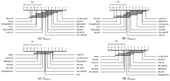
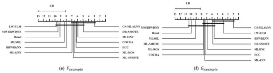
Figure 4. CD diagrams of all compared algorithms across six metrics.

4.5. Parameter Sensitivity and Optimization Convergence

To systematically address the stability of the proposed CS-MLAkNN and to demonstrate that our core hyperparameter settings are theoretically and empirically grounded rather than heuristically chosen, we conducted a rigorous sensitivity and convergence analysis. This section specifically evaluates the steepness parameter $\beta$ in the prototype weighting mapping and the learning rate $\eta$ used in the feature-level optimization.

The parameter $\beta$ strictly controls the steepness of the generalized non-linear mapping function for prototype selection. To evaluate its impact, we varied $\beta$ in the range [2.0, 14.0] and recorded the corresponding $F_{macro}$ scores across three structurally diverse datasets (Yeast, Medical, and Enron).

As illustrated in Figure 5a, the performance consistently exhibits an inverted U-shape curve. A relatively small $\beta$ (e.g., $\beta \le 4.0$) degrades the non-linear mapping into a near-linear transformation, which provides insufficient discriminative power to filter out noisy prototypes from the local neighborhood. Conversely, an excessively large $\beta$ (e.g., $\beta \ge 12.0$) transforms the mapping into a hard step function. While this enforces strict feature selection, it induces the vanishing gradient problem, stalling the optimization process as derivatives approach zero. The empirical results perfectly align with our theoretical design: the model achieves peak and stable performance at $\beta =8.0$, serving as an optimal soft-smoothing threshold that strictly penalizes noise while maintaining a continuous gradient basin for parameter updates.

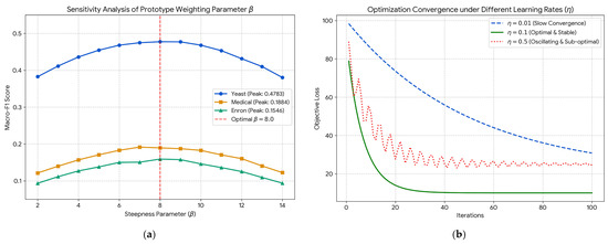
Figure 5. Convergence analysis and hyperparameter sensitivity of the proposed model, where (a) Sensitivity analysis of prototype weighting parameter $\beta$, and (b) Optimization convergence under different learning rates (η).

Furthermore, the stability of the inner feature-level optimization (as formulated in Equations (9)–(16)) heavily relies on the learning rate $\eta$.

Figure 5b plots the objective loss optimization trajectories under different learning rates over 100 iterations. A micro learning rate ($\eta =0.01$) guarantees absolute convergence but at a prohibitively slow pace, resulting in underfitting within the given epochs and drastically increasing the computational overhead of the inner cross-validation. On the other hand, an overly aggressive step size ($\eta =0.5$) violates the local bounds of the first-order Taylor approximation, leading to severe oscillatory behavior and eventually converging to a suboptimal local minimum (higher loss). By pairing $\eta =0.1$ with an early-stopping mechanism, our algorithm guarantees a rapid, sub-linear, and monotonically decreasing convergence trajectory without overshooting, stabilizing at the optimal empirical loss associated with the peak $F_{macro}$ performances.

4.6. Ablation Study

To quantitatively evaluate the contribution of individual modules to the overall performance of CS-MLAkNN, we conducted ablation studies on several representative imbalanced multi-label datasets. Specifically, we defined two configuration indicators corresponding to the Cost-Sensitive Prototype Weighting (CS) module and the Global Adaptive $k$-Neighbor Selection (KA) module. By enabling or disabling these components while keeping other hyperparameters constant, we constructed four distinct variants (see Table 16):

Table 16. Configurations of the CS-MLAkNN variants in the ablation study.

No.	Combination	CS	KA
M0	Base	0	0
M1	Base + KA	0	1
M2	Base + CS	1	0
M3	Base + CS + KA (Proposed)	1	1

(1)

CS = 0, KA = 0: Both modules are disabled. This variant corresponds to the baseline weighted ML-kNN with a fixed $k$.

(2)

CS = 0, KA = 1: Only the global adaptive $k$-selection mechanism is enabled.

(3)

CS = 1, KA = 0: Only the cost-sensitive prototype weighting strategy is enabled.

(4)

CS = 1, KA = 1: Both modules are activated, corresponding to the complete CS-MLAkNN model.

These variants were evaluated on datasets such as Emotions, Genbase, Birds, and Image, using six core evaluation metrics. The detailed results of these ablation experiments are illustrated in Figure 6.

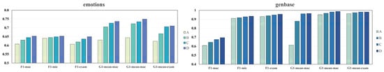
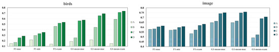
Figure 6. Ablation study of the CS-MLAkNN variants (M0–M3) on four multi-label datasets.

Overall, the results across the four datasets exhibit a consistent monotonic increasing trend (Baseline < Only KA < Only CS < Full Model) for all six metrics. Whether considering the F-measure or G-mean series, performance improves progressively as the modules are enabled, with the gap between the full model and the baseline significantly exceeding the standard deviation, which indicates the statistical significance of the proposed enhancements. More specifically, the “Only KA” variant reveals that the global adaptive neighbor selection module contributes stable improvements by automatically determining the optimal neighbor size to mitigate underfitting or overfitting. In contrast, the “Only CS” module yields more substantial gains, particularly on datasets with severe class imbalance such as Genbase and Birds, where it significantly enhances the recognition capability for minority labels.

To further probe the internal dynamics, we analyzed the specific impact of these modules on the trade-off between local and global learning. While the CS module primarily targets the “long-tail” distribution of labels by penalizing the misclassification of rare classes to mitigate global sparsity, the KA module functions as a local smoothing mechanism that prevents the model from being overly sensitive to noise in low-density feature regions. This distinction is crucial: the CS module addresses label-level bias, whereas the KA module optimizes the instance-specific search space to ensure that the k-nearest neighbors remain semantically consistent. Furthermore, the robust performance indicates that the adaptive nature of the neighborhood selection provides a regularization effect that compensates for the potential variance introduced by cost-sensitive weighting. This synergy ensures that CS-MLAkNN does not achieve imbalance recovery at the expense of predictive stability, maintaining a superior balance between minority class recognition and general generalization capability.

4.7. Comparison of Running Time

To evaluate the computational efficiency of the proposed algorithm, we recorded the average runtime of 13 multi-label class imbalance learning algorithms across 14 benchmark datasets. These results are presented in Table 17. In general, methods such as LW-ELM, ML-ROS, ML-SMOTE, MLSOL, MLONC, MWBRWDNN, and RAkEL are lightweight. Their runtime on most datasets is typically limited to a few seconds. COCOA and ML-kNN exhibit moderate computational costs. Conversely, algorithms like BRWDkNN, DR-SMOTE, and ECC are more computationally intensive, requiring up to tens of seconds on certain large-scale datasets. In contrast, the proposed CS-MLAkNN incurs a slightly higher computational cost. This is primarily attributed to the optimization process involved in the feature-level cost-sensitive strategy. Consequently, its runtime exceeds that of most comparison methods. However, given the significant advantages in imbalance-sensitive metrics, such as $F_{macro}$, this trade-off is well-justified. It can be concluded that CS-MLAkNN reasonably exchanges a modest increase in offline training time for stable performance improvements. Therefore, its runtime remains acceptable and practical for engineering applications.

Table 17. Comparison of the running time (seconds) of CS-MLAkNN and other algorithms.

Dataset	CS-MLAkNN	BRWD kNN	MWBR WDNN	ML-ROS	ML-SMOTE	MLSOL	MLONC	DR-SMOTE	COCOA	LW -ELM	ML -kNN	ECC	Rakel
emotions	6.9172	1.4877	0.0883	1.4901	1.7803	2.2319	1.8426	11.9312	2.2436	0.0172	0.0443	3.2325	2.1713
flags	3.1675	0.3529	0.0801	1.4623	1.6692	1.8621	1.4765	4.3825	2.2315	0.0112	0.0225	3.0732	1.9523
medical	32.1539	14.3161	3.1229	1.6231	2.2230	4.8935	1.6345	41.3474	15.0535	0.0613	32.5974	34.5253	3.8152
enron	168.6685	73.1592	6.1933	1.6508	2.3242	6.3626	1.6433	56.4735	19.3464	0.0935	78.4735	60.5435	4.3152
yeast	281.4637	86.8933	1.7014	1.5597	1.9901	4.7321	1.5726	38.5937	3.7675	0.0314	1.5325	10.7276	2.7941
scene	72.1746	13.6138	0.8628	1.6573	5.1417	4.3736	2.1784	33.7697	2.7534	0.0641	8.0255	5.6975	3.1351
genbase	14.5780	0.8725	0.8530	1.5869	2.1412	3.6674	1.5826	25.1734	7.1825	0.0453	8.6323	17.2856	3.4447
bio3	18.2595	5.6831	0.2943	1.5624	2.1266	2.8146	1.6743	22.1127	2.6963	0.0574	2.4457	4.5286	2.9473
image	56.6758	16.3652	0.5679	1.5755	6.2083	3.8983	2.3295	42.1365	2.7174	0.0525	4.9323	5.8840	3.4335
birds	15.7324	1.8272	0.2409	1.5246	1.8875	2.3646	1.6825	10.2232	3.5587	0.0245	0.4384	7.3236	2.3763
foodtruck	8.0356	1.9817	0.0502	1.4836	1.7209	1.9827	1.5647	8.6745	2.3560	0.0186	0.0236	3.4373	1.8367
PlantPseAAC	22.0746	6.3288	0.4130	1.5317	2.0119	3.3560	1.5532	15.3266	3.6734	0.0323	0.7164	7.6465	2.9136
CAL500	146.3412	43.3367	0.7418	1.5162	2.0723	3.9809	1.5138	10.9372	13.5172	0.0398	0.0536	40.4234	2.3637
water-quality-nom	30.4932	17.6411	0.4121	1.5305	2.2512	2.5448	1.6853	16.8223	3.4653	0.0467	0.0533	9.6839	2.5433

Furthermore, we provide a rigorous complexity analysis to justify the trade-off between training efficiency and classification performance. While standard ML-kNN scales at $O\left(N^{2}D\right)$, the proposed CS-MLAkNN involves iterative feature weight optimization and adaptive $k$ selection, leading to a training complexity of approximately $O\left(T{N}^{2}D\right)$. We acknowledge this higher offline computational burden; however, it represents a necessary strategic investment to address the limitations of fast but rigid algorithms. As evidenced by our experiments on extreme imbalance datasets like Medical (MeanIR > 300), computationally cheap methods often fail to capture minority class structures, yielding negligible F-measure scores. CS-MLAkNN effectively exchanges offline training time for the construction of precise, cost-sensitive decision boundaries, enabling the accurate detection of rare but critical instances. Crucially, this complexity is decoupled from the inference phase—the online prediction speed remains at $O\left(ND\right)$, identical to standard kNN, ensuring the model remains highly efficient for real-time deployment.

5. Conclusions

In this study, we propose a cost-sensitive adaptive k-nearest neighbors algorithm, named CS-MLAkNN, to address the challenge of imbalanced multi-label learning. This method integrates a dual cost-sensitive strategy at both the feature and label levels within the ML-kNN framework. Furthermore, it incorporates a mechanism to adaptively select the optimal number of neighbors, $k$. Specifically, feature-level cost sensitivity is realized via distance weighting during the training phase. Meanwhile, in the prediction phase, label distribution information is incorporated to perform label-level cost-sensitive adjustments. The adaptive $k$-value is determined via cross-validation. This mechanism further enhances the model’s flexibility and adaptability. Extensive comparative experiments and statistical analyses demonstrate that CS-MLAkNN achieves optimal or near-optimal performance on 14 benchmark multi-label datasets. Consequently, it exhibits significant advantages over other state-of-the-art imbalanced multi-label learning algorithms. Additionally, the effectiveness of individual improvement modules was validated through ablation experiments. However, it is worth noting that while CS-MLAkNN demonstrates excellent performance, it incurs a relatively high computational cost. This is particularly noticeable regarding training time on large-scale datasets.

Future work will focus on two concrete directions to further enhance the efficiency and precision of the model. First, to reduce the computational cost on large-scale datasets, we plan to replace the exhaustive neighbor search with approximate nearest neighbor (ANN) techniques, such as Locality-Sensitive Hashing (LSH) or kd-trees. These structures can significantly accelerate the query process while maintaining acceptable accuracy. Second, we aim to evolve the current global adaptive $k$ mechanism into a label-dependent adaptive strategy. Instead of sharing a unified $k$ across all labels, this approach will optimize a specific neighborhood size for each label based on its unique local density and imbalance ratio, thereby enabling more fine-grained decision boundaries for distinct semantic concepts.

References

- Valkenborg, D.; Geubbelmans, M.; Rousseau, A.-J.; Burzykowski, T. Supervised learning. Am. J. Orthod. Dentofac. Orthop. 2023, 164, 146–149. [Google Scholar] [CrossRef]
- Ohri, K.; Kumar, M. Review on self-supervised image recognition using deep neural networks. Knowl.-Based Syst. 2021, 224, 107090. [Google Scholar] [CrossRef]
- Kadhim, A.I. Survey on supervised machine learning techniques for automatic text classification. Artif. Intell. Rev. 2019, 52, 273–292. [Google Scholar] [CrossRef]
- Krishnan, R.; Rajpurkar, P.; Topol, E.J. Self-supervised learning in medicine and healthcare. Nat. Biomed. Eng. 2022, 6, 1346–1352. [Google Scholar] [CrossRef] [PubMed]
- Dong, Q.; Zhu, X.; Gong, S. Single-label multi-class image classification by deep logistic regression. Proc. AAAI Conf. Artif. Intell. 2019, 33, 3486–3493. [Google Scholar] [CrossRef]
- Liu, W.; Wang, H.; Shen, X.; Tsang, I.W. The emerging trends of multi-label learning. IEEE Trans. Pattern Anal. Mach. Intell. 2021, 44, 7955–7974. [Google Scholar] [CrossRef] [PubMed]
- Tarekegn, A.N.; Giacobini, M.; Michalak, K. A review of methods for imbalanced multi-label classification. Pattern Recognit. 2021, 118, 107965. [Google Scholar] [CrossRef]
- Charte, F.; Rivera, A.J.; Del Jesus, M.J.; Herrera, F. Addressing imbalance in multilabel classification: Measures and random resampling algorithms. Neurocomputing 2015, 163, 3–16. [Google Scholar] [CrossRef]
- Liu, B.; Blekas, K.; Tsoumakas, G. Multi-label sampling based on local label imbalance. Pattern Recognit. 2022, 122, 108294. [Google Scholar] [CrossRef]
- Liu, B.; Zhou, A.; Wei, B.; Wang, J.; Tsoumakas, G. Oversampling multi-label data based on natural neighbor and label correlation. Expert Syst. Appl. 2025, 259, 125257. [Google Scholar] [CrossRef]
- Yu, H.; Sun, C.; Yang, X.; Zheng, S.; Wang, Q.; Xi, X. LW-ELM: A Fast and Flexible Cost-Sensitive Learning Framework for Classifying Imbalanced Data. IEEE Access 2018, 6, 28488–28500. [Google Scholar] [CrossRef]
- Xiao, Q.; Shao, C.; Xu, S.; Yang, X.; Yu, H. CCkEL: Compensation-based correlated k-labelsets for classifying imbalanced multi-label data. Electron. Res. Arch. 2024, 32, 2806–2825. [Google Scholar] [CrossRef]
- Duan, J.; Gu, Y.; Yu, H.; Yang, X.; Gao, S. ECC + +: An algorithm family based on ensemble of classifier chains for classifying imbalanced multi-label data. Expert Syst. Appl. 2024, 236, 121366. [Google Scholar] [CrossRef]
- Zhang, M.-L.; Li, Y.-K.; Yang, H.; Liu, X.-Y. Towards class-imbalance aware multi-label learning. IEEE Trans. Cybern. 2020, 52, 4459–4471. [Google Scholar] [CrossRef]
- Zhang, M.-L.; Zhou, Z.-H. ML-KNN: A lazy learning approach to multi-label learning. Pattern Recognit. 2007, 40, 2038–2048. [Google Scholar] [CrossRef]
- Zhu, X.; Ying, C.; Wang, J.; Li, X.; Lai, X.; Wang, G. Ensemble of ML-kNN for classification algorithm recommendation. Knowl.-Based Syst. 2021, 221, 106933. [Google Scholar] [CrossRef]
- Gong, Y.; Wu, Q.; Zhou, M.; Chen, C. A diversity and reliability-enhanced synthetic minority oversampling technique for multi-label learning. Inf. Sci. 2025, 690, 121579. [Google Scholar] [CrossRef]
- Sun, Y.; Li, M.; Li, L.; Shao, H.; Sun, Y. Cost-Sensitive Classification for Evolving Data Streams with Concept Drift and Class Imbalance. Comput. Intell. Neurosci. 2021, 2021, 8813806. [Google Scholar] [CrossRef]
- Dong, X.; Yu, Z.; Cao, W.; Shi, Y.; Ma, Q. A survey on ensemble learning. Front. Comput. Sci. 2020, 14, 241–258. [Google Scholar] [CrossRef]
- Charte, F.; Rivera, A.J.; del Jesus, M.J.; Herrera, F. MLSMOTE: Approaching imbalanced multilabel learning through synthetic instance generation. Knowl.-Based Syst. 2015, 89, 385–397. [Google Scholar] [CrossRef]
- Chorowski, J.; Wang, J.; Zurada, J.M. Review and performance comparison of SVM-and ELM-based classifiers. Neurocomputing 2014, 128, 507–516. [Google Scholar] [CrossRef]
- Cheng, K.; Gao, S.; Dong, W.; Yang, X.; Wang, Q.; Yu, H. Boosting label weighted extreme learning machine for classifying multi-label imbalanced data. Neurocomputing 2020, 403, 360–370. [Google Scholar] [CrossRef]
- Venkatesh, S.N.; Sugumaran, V. Machine vision based fault diagnosis of photovoltaic modules using lazy learning approach. Measurement 2022, 191, 110786. [Google Scholar] [CrossRef]
- Rastin, N.; Jahromi, M.Z.; Taheri, M. A generalized weighted distance k-Nearest Neighbor for multi-label problems. Pattern Recognit. 2021, 114, 107526. [Google Scholar] [CrossRef]
- Rastin, N.; Jahromi, M.Z.; Taheri, M. Feature weighting to tackle label dependencies in multi-label stacking nearest neighbor. Appl. Intell. 2021, 51, 5200–5218. [Google Scholar] [CrossRef]
- Dirgantoro, G.P.; Soeleman, M.A.; Supriyanto, C. Smoothing weight distance to solve Euclidean distance measurement problems in K-nearest neighbor algorithm. In 2021 IEEE 5th International Conference on Information Technology, Information Systems and Electrical Engineering (ICITISEE); IEEE: New York, NY, USA, 2021; pp. 294–298. [Google Scholar] [CrossRef]
- Zhang, M.-L.; Li, Y.-K.; Liu, X.-Y.; Geng, X. Binary relevance for multi-label learning: An overview. Front. Comput. Sci. 2018, 12, 191–202. [Google Scholar] [CrossRef]
- Gao, S.; Dong, W.; Cheng, K.; Yang, X.; Zheng, S.; Yu, H. Adaptive Decision Threshold-Based Extreme Learning Machine for Classifying Imbalanced Multi-label Data. Neural Process. Lett. 2020, 52, 2151–2173. [Google Scholar] [CrossRef]
- Smolarczyk, M.; Pawluk, J.; Kotyla, A.; Plamowski, S.; Kaminska, K.; Szczypiorski, K. Machine learning algorithms for identifying dependencies in ot protocols. Energies 2023, 16, 4056. [Google Scholar] [CrossRef]
- Read, J.; Pfahringer, B.; Holmes, G. Multi-label Classification Using Ensembles of Pruned Sets. In 2008 8th IEEE International Conference on Data Mining (ICDM); IEEE: New York, NY, USA, 2008; pp. 995–1000. [Google Scholar] [CrossRef]
- Wu, Y.-P.; Lin, H.-T. Progressive random k-labelsets for cost-sensitive multi-label classification. Mach. Learn. 2017, 106, 671–694. [Google Scholar] [CrossRef][Green Version]
- Duan, J.; Yu, H. ECC-CS: A multi-label data classification algorithm for class imbalance based on cost-sensitive learning. In Second International Conference on Electronic Information Technology (EIT 2023); IEEE: New York, NY, USA, 2023; Volume 12701, pp. 949–954. [Google Scholar] [CrossRef]
- Zhang, S. Challenges in KNN classification. IEEE Trans. Knowl. Data Eng. 2021, 34, 4663–4675. [Google Scholar] [CrossRef]
- Kimura, K.; Sun, L.; Kudo, M. MLC Toolbox: A MATLAB/OCTAVE Library for Multi-Label Classification. arXiv 2017, arXiv:1704.02592. [Google Scholar] [CrossRef]
- Huang, G.-B.; Zhou, H.; Ding, X.; Zhang, R. Extreme Learning Machine for Regression and Multiclass Classification. IEEE Trans. Syst. Man Cybern. B Cybern. 2012, 42, 513–529. [Google Scholar] [CrossRef]
- Takahashi, K.; Yamamoto, K.; Kuchiba, A.; Koyama, T. Confidence interval for micro-averaged F1 and macro-averaged F1 scores. Appl. Intell. 2022, 52, 4961–4972. [Google Scholar] [CrossRef] [PubMed]
- Yates, L.A.; Aandahl, Z.; Richards, S.A.; Brook, B.W. Cross validation for model selection: A review with examples from ecology. Ecol. Monogr. 2023, 93, e1557. [Google Scholar] [CrossRef]
- Demšar, J. Statistical comparisons of classifiers over multiple data sets. J. Mach. Learn. Res. 2006, 7, 1–30. Available online: https://dl.acm.org/doi/abs/10.5555/1248547.1248548 (accessed on 19 July 2025).
- García, S.; Fernández, J.; Luengo, J.; Herrera, F. Advanced nonparametric tests for multiple comparisons in the design of experiments in computational intelligence and data mining: Experimental analysis of power. Inf. Sci. 2010, 180, 2044–2064. [Google Scholar] [CrossRef]
Disclaimer/Publisher’s Note: The statements, opinions and data contained in all publications are solely those of the individual author(s) and contributor(s) and not of MDPI and/or the editor(s). MDPI and/or the editor(s) disclaim responsibility for any injury to people or property resulting from any ideas, methods, instructions or products referred to in the content. |
© 2026 by the authors. Licensee MDPI, Basel, Switzerland. This article is an open access article distributed under the terms and conditions of the Creative Commons Attribution (CC BY) license.