Symmetry-Aware Dynamic Graph Learning for One-Step Scenic-Spot Visitor Demand Forecasting

Abstract

Accurate one-step forecasting of scenic-spot visitor demand is challenging due to strong non-stationarity, holiday-induced peaks, and abrupt reputation-driven shocks. We propose a symmetry-aware dynamic graph learning framework that fuses social–physical sensing streams for robust demand prediction. Online reviews are treated as social sensing, transformed into daily sentiment indicators, and aligned with demand using a delay-aware aggregation scheme. To capture evolving inter-spot dependencies, we construct a time-varying adjacency matrix that is updated over time and integrated into a lightweight spatio-temporal forecasting model, Dynamic Spatio-temporal Graph Attention LSTM (DSGAT-LSTM). The model preserves the permutation-invariant property of graph learning while introducing sentiment-guided feature reweighting and sentiment-gated temporal updates to better track volatility. Experiments on multi-year daily data from multiple A-level scenic spots with holiday and weather context demonstrate consistent error reductions over representative temporal and graph-based baselines, together with improved stability under peak and shock conditions. We will release the processed feature-level dataset and implementation scripts to support reproducibility.

1. Introduction

Accurate one-step forecasting of scenic-spot visitor demand is a practical yet challenging spatio-temporal prediction problem, where observations are collected from heterogeneous sensing sources and must be integrated into a coherent computational model. In real deployments, demand time series are strongly non-stationary and can exhibit sharp peaks and abrupt shocks, driven by contextual factors (e.g., holidays and weather) and by changes in perceived experience reflected in online reviews [1]. From a machine learning and algorithmic perspective, the key difficulty is to model evolving inter-spot dependence with structural consistency: the predictive mechanism should be invariant to the permutation of scenic-spot indices while still capturing time-varying interactions represented by a dynamic adjacency matrix. These requirements motivate symmetry-aware dynamic graph learning that combines multi-source information processing with robust spatio-temporal modeling, enabling stable short-horizon forecasting and reliable decision support under rapidly changing conditions.

From the perspective of geospatial artificial intelligence, this problem goes beyond improving a single time-series predictor. It requires learning from multiple geo-referenced observations that are generated by different processes and arrive at different times. Besides physical sensing, tourists continuously contribute large-scale social sensing signals through online reviews and other user-generated content. These signals complement on-site counts because they reflect perceived experience, latent satisfaction, and emerging complaints that are not visible in flow measurements alone. Prior work has shown that sentiment features extracted from reviews can improve demand forecasting, especially during disruptive periods when behavioral patterns deviate from historical regularities [2,3]. Multimodal content, such as user-generated images on online travel agency (OTA) platforms, can also carry predictive cues that are difficult to capture with numerical streams [4,5]. A central obstacle is temporal misalignment: reviews are often posted after visits, and naively attaching review sentiment to the posting date can introduce noise and reduce stability.

Equally important, scenic spots form an interacting geographic system rather than independent units. Tourists commonly visit multiple attractions within an itinerary, and substitution, complementarity, and crowd redistribution create inter-spot dependence that changes over time with accessibility, policies, events, and shifting preferences. Many tourism forecasting pipelines either model each spot in isolation or assume static correlations, and such assumptions can break during peak seasons and sudden shocks. Recent advances in spatio-temporal graph neural networks provide a principled way to couple spatial dependence with temporal dynamics [6,7,8,9]. Surveys in urban and geospatial predictive learning further highlight the need for dynamic and heterogeneous graph modeling to represent evolving interactions in real systems [10,11]. [12] develops a system-level, modular remediation framework that reframes legacy landfills as resilience assets, providing actionable insights for buffering critical AI loads amid grid volatility. In geoinformation settings, spatial dependence is often grounded in geographic proximity and accessibility, and it can be enriched by contextual layers that are routinely available from meteorological products and remote-sensing observations. This motivates graph structures that can evolve while remaining consistent with geographic constraints.

Meanwhile, reproducible public resources related to tourism data are growing, but they remain fragmented across tasks. Recent datasets focus on context-aware route recommendation (e.g., Context Trails) [5,13] or large-scale semantic trajectories for point of interest (POI) recommendation benchmarks (e.g., Massive-STEPS) [14]. [15] establishes a location-robust, cost-preserving blended pricing framework that reconciles accounting identity with decision-stable signals across geographically heterogeneous AI data center campuses. These resources are valuable for studying routes and preferences, yet they are not designed for sensor-plus-social demand forecasting at scenic spots. They also rarely provide an end-to-end pipeline that connects sensing streams, review-derived sentiment, time-varying interaction graphs, and short-horizon predictions in a unified geospatial learning setting. This gap motivates a framework that can fuse heterogeneous signals, correct for review-delay effects, and learn evolving inter-spot interactions in a way that is compatible with geospatial context layers, including those derived from remote sensing.

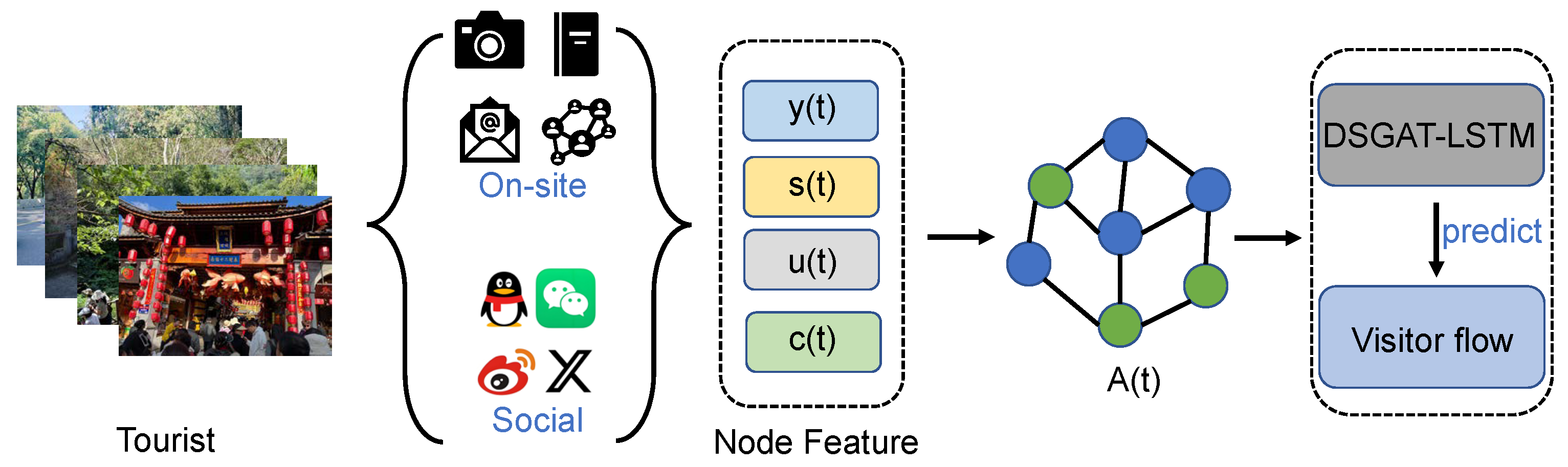
In this work, we formulate scenic-spot visitor demand forecasting as a sentiment-aware graph learning problem under a social–physical sensing setting (Figure 1). We treat online reviews as social sensing signals and derive daily sentiment indicators with a delay-aware alignment to obtain temporally consistent features. We integrate holiday and weather context, and we learn a time-varying adjacency to reflect evolving inter-spot interactions. Building on these components, we develop a lightweight forecasting model, Dynamic Spatio-temporal Graph Attention LSTM (DSGAT-LSTM), which improves prediction accuracy and maintains stable performance during peak and shock periods.

The main contributions of this paper are summarized as follows:

• We present a geoinformation-oriented formulation (i.e., scenic spots as geo-referenced nodes with a distance-based proximity prior and geospatially available context) for daily one-step scenic-spot demand forecasting that fuses on-site flow observations, review-derived social sensing, and contextual drivers such as holiday and weather.
• We design a delay-aware alignment strategy that transforms asynchronous review texts into temporally consistent daily sentiment signals, enabling reliable fusion with sensing-derived demand series.
• We introduce a time-varying adjacency mechanism for inter-spot dependency modeling, allowing connectivity to evolve with observed interactions while remaining compatible with geographic relationships among scenic spots.
• We develop a lightweight DSGAT-LSTM model that combines sentiment-guided feature modulation, graph-attention-based spatial aggregation on a time-varying graph, and temporal sequence modeling for robust short-horizon forecasting.

2. Related Work

2.1. Tourism Demand Forecasting with Contextual Variables

Tourism demand forecasting has long relied on statistical time-series models and has increasingly shifted toward machine learning and deep learning approaches that capture non-linear dynamics and incorporate exogenous drivers. Recent temporal architectures, including attention-based sequence models, have improved the ability to fuse heterogeneous covariates and offer more flexible representations for operational forecasting [16]. In scenic-spot management, holiday and weather variables are widely recognized as primary external drivers, yet they do not fully explain abrupt demand changes caused by evolving travel preferences and experience shocks. Moreover, many studies still model each attraction independently, which can overlook the coupled nature of multi-spot itineraries and substitution or complementarity effects across attractions. As a result, models can become less reliable during extreme periods, precisely when short-horizon predictions are most valuable for crowd monitoring and decision support.

2.2. Sensor-Based Crowd Monitoring and Tourism Mobility Sensing

The deployment of smart tourism infrastructure has enabled sensing-driven crowd monitoring and mobility analytics. Prior work has explored how sensing streams such as Wi-Fi probing can support tourism analytics and recommendation while addressing privacy considerations and data utility trade-offs [1,15]. Related studies have further demonstrated that passive sensing signals can serve as proxies for visitor presence and movement patterns and can be used to derive behavioral indicators for downstream applications [17,18]. In addition to model design, recent control-inspired optimization methods have shown that layer-wise adaptive update rules can significantly improve learning efficiency, offering complementary perspectives for training deep models [19]. Despite their timeliness and objectivity, physical sensing signals are constrained by deployment coverage and can be affected by sampling bias, device heterogeneity, and privacy-preserving mechanisms. These limitations motivate complementary information sources that capture aspects not directly observable from sensors, such as perceived experience and satisfaction.

2.3. Social Sensing from Reviews and User-Generated Content

Online reviews and other user-generated content provide a social sensing perspective that reflects perceived experience and latent satisfaction trends. Sentiment signals extracted from reviews have been shown to improve tourism forecasting, particularly when demand fluctuations are driven by experience-related factors rather than purely seasonal regularities [2]. Beyond text, multimodal UGC such as user-generated images on OTA platforms has also been investigated as predictive evidence that complements numerical sensing records [4]. A practical challenge is that review posting is asynchronous with respect to visits, and the delay pattern can vary across platforms and event contexts. Consequently, naive feature aggregation by posting day may introduce temporal mismatch and noise. Existing tourism forecasting studies often treat sentiment as an additional covariate, but fewer explicitly model posting delays or jointly incorporate semantic representations and cross-spot dependence in a unified short-horizon forecasting pipeline.

2.4. Spatio-Temporal Graph Forecasting and Dynamic Dependency Learning

Spatio-temporal graph neural networks (STGNNs) have become a powerful paradigm for forecasting in networked systems by coupling spatial aggregation on graphs with temporal modeling. Representative methods such as diffusion convolutional recurrent neural network (DCRNN) and STGCN demonstrate that graph-based spatial propagation combined with recurrent or convolutional temporal modules can improve predictive accuracy when entities are interdependent [6,7]. Attention-based variants further enhance flexibility by learning non-uniform spatial influence [8]. Recent surveys highlight that real-world forecasting often requires handling heterogeneous inputs, robustness constraints, and potentially time-varying relations [10,11,12,20]. To address unknown or evolving connectivity, adaptive and learned graph mechanisms have been proposed, including Graph WaveNet with learnable dependency structures [21], node-adaptive graph generation in AGCRN [22], and directed dependency learning in MTGNN [23]. Dynamic-graph modeling has also been studied via evolving parameterizations (e.g., EvolveGCN) [24] and continuous-time formulations (e.g., STGODE) [25].

Most STGNN validations are conducted on transportation or traffic benchmarks where topology and interactions follow infrastructure constraints. In tourism forecasting, inter-spot relations can change with itineraries, policies, and seasonal regimes, and experience-related signals (e.g., sentiment and semantic cues) can trigger demand shifts. This setting calls for a modeling strategy that simultaneously accounts for dynamic dependency learning and the temporal characteristics of social sensing signals.

2.5. Geospatial AI and Remote-Sensing-Compatible Covariates for Demand Modeling

Geospatial artificial intelligence increasingly emphasizes learning from heterogeneous geo-referenced signals, where point-based observations can be complemented by spatially continuous environmental covariates. In tourism demand modeling, meteorological drivers and broader environmental conditions can be represented not only by station records but also by gridded products, such as reanalysis fields or remote-sensing-derived climate and surface variables, which offer consistent spatial coverage and support transfer to regions with sparse in-situ measurements. From a methodological perspective, representing scenic spots as geo-referenced nodes and introducing a coordinate-derived proximity prior provides a natural interface for incorporating such gridded covariates through spatial sampling or neighborhood aggregation around each POI [26,27,28]. This compatibility is particularly relevant for operational geoinformation systems, where multi-source sensing and environmental layers are routinely managed in a unified spatio-temporal framework. In this context, models that jointly account for temporal dynamics, spatial interactions, and heterogeneous covariates are better aligned with the goals of GeoAI-driven decision support.

2.6. Public Tourism Datasets and Benchmarks

Public resources for tourism data are growing, especially for recommendation and mobility modeling. Context Trails provides tourism trails enriched with contextual factors and supports evaluation for contextual and route recommendation [13,29,30,31]. Massive-STEPS offers large-scale semantic trajectories for POI modeling and benchmarking [14]. These datasets facilitate reproducibility for recommendation-related tasks, but they are not directly tailored to daily scenic-spot demand forecasting that fuses on-site sensing, review-derived social sensing, holiday–weather context, and time-varying cross-spot interactions. In particular, the combination of operational sensing-derived demand series with asynchronous review streams and dynamic inter-spot dependency learning remains less covered by existing benchmarks.

2.7. Positioning of Our Work

Our work lies at the intersection of tourism demand forecasting, geospatial sensing, and dynamic spatio-temporal graph learning. Different from approaches that forecast each scenic spot independently using only historical demand and context, we explicitly model cross-spot interactions through a daily updated adjacency that combines a coordinate-derived geospatial proximity prior with short-term interaction patterns inferred from recent demand dynamics [3]. Different from general STGNN forecasting pipelines, we incorporate social sensing signals extracted from online reviews in two complementary forms, namely aligned daily sentiment and compact semantic representations, and we adopt a delay-aware alignment strategy to mitigate asynchronous posting behavior. These design choices support a unified social–physical sensing framework for robust one-step forecasting, with particular attention to peak-demand and shock scenarios relevant to real-world scenic-spot management.

3. Methodology

3.1. Problem Setup

Motivated by these insights, we structure our pipeline into modular components (social-sensing extraction, delay-aware alignment, dynamic graph construction, and lightweight spatio-temporal forecasting) and explicitly incorporate robustness-oriented choices to support stable operation under heterogeneous and non-stationary conditions. We model N scenic spots as geo-referenced nodes in a spatial system. Each spot $i\in \{1,\dots ,N\}$ is associated with a location $({\phi }_i,{\lambda }_i)$, where ${\phi }_i$ and ${\lambda }_i$ denote latitude and longitude (in radians). On day t, the observed visitor demand at spot i is $y_i\left(t\right)$, and the exogenous context is summarized by a vector $\mathbf{c}\left(t\right)$, which includes holiday indicators and meteorological variables (e.g., temperature and precipitation). Online reviews are denoted by a stream $\mathcal{R}$, where each review k is associated with a spot index $i_k$ and a posting day $t_k$.

Given historical observations up to day t, our goal is to forecast the one-day-ahead demand:

$$\widehat{\mathbf{y}}(t+1)=f_{\mathsf{\Theta }}\left({\left\{\mathbf{y}\left(\tau \right)\right\}}_{\tau \le t},{\mathcal{R}}_{\tau \le t},{\left\{\mathbf{c}\left(\tau \right)\right\}}_{\tau \le t}\right),$$

(1)

where $\mathbf{y}\left(t\right)={[y_1\left(t\right),\dots ,y_N\left(t\right)]}^{\top }$, $\widehat{\mathbf{y}}(t+1)={[{\widehat{y}}_1(t+1),\dots ,{\widehat{y}}_N(t+1)]}^{\top }$, and $\mathsf{\Theta }$ denotes trainable parameters.

3.2. Social Sensing: Review-Level Sentiment and Embedding

We treat online reviews as social sensing signals that complement physical flow observations. Each review text $r_k$ is mapped to (i) a scalar sentiment score $s_k\in [-1,1]$ and (ii) a dense embedding ${\mathbf{e}}_k\in {\mathbb{R}}^{d_e}$:

$$(s_k,{\mathbf{e}}_k)=\mathsf{\Phi }\left(r_k\right).$$

(2)

We view $\mathsf{\Phi }(·)$ as a neural text encoder that outputs a contextual representation ${\mathbf{z}}_k\in {\mathbb{R}}^{d_e}$ together with a sentiment regression head:

$${\mathbf{e}}_k={\mathbf{z}}_k,s_k=2\sigma ({\mathbf{w}}_{\mathrm{sent}}^{\top }{\mathbf{z}}_k+b_{\mathrm{sent}})-1,$$

(3)

where $\sigma (·)$ is the sigmoid function and $({\mathbf{w}}_{\mathrm{sent}},b_{\mathrm{sent}})$ are parameters of the sentiment head.

3.3. Delay-Aware Alignment: Daily Sentiment Signal $s_i\left(t\right)$

Reviews are often posted after the actual visit, so directly aligning sentiment to the posting day can introduce noise. We build a delay-aware daily sentiment signal by aggregating reviews in a backward window of length $\Delta$:

$${\mathcal{R}}_i\left(t\right)=\left\{k|i_k=i,t-\Delta \le t_k\le t\right\}.$$

(4)

We assign higher weights to more recent reviews using an exponential kernel:

$$w_k\left(t\right)=exp\left(-{\lambda }_r(t-t_k)\right),$$

(5)

where ${\lambda }_r>0$ controls how fast older reviews decay. The aligned daily sentiment is defined as

$$s_i\left(t\right)=\left\{\begin{array}{cc}{\displaystyle \frac{{\sum }_{k\in {\mathcal{R}}_i\left(t\right)}{w}_k\left(t\right)s_k}{{\sum }_{k\in {\mathcal{R}}_i\left(t\right)}{w}_k\left(t\right)+ϵ}},\hfill & |{\mathcal{R}}_i\left(t\right)|>0,\hfill \\ s_i(t-1),\hfill & |{\mathcal{R}}_i\left(t\right)|=0\mathrm{and}t>1,\hfill \\ 0,\hfill & |{\mathcal{R}}_i\left(t\right)|=0\mathrm{and}t=1,\hfill \end{array}\right.$$

(6)

where $ϵ$ is a small constant for numerical stability.

3.4. Daily Review Representation $u_i\left(t\right)$ and Feature Fusion

Beyond a scalar sentiment score, reviews contain semantic cues that may be predictive. We summarize these cues using a compact daily representation ${\mathbf{u}}_i\left(t\right)\in {\mathbb{R}}^{d_e}$ obtained from aligned review embeddings.

We compute attention weights over reviews in ${\mathcal{R}}_i\left(t\right)$ and incorporate the same delay weights to maintain temporal consistency:

$${\tilde{\pi }}_k\left(t\right)=w_k\left(t\right)·exp\left({\mathbf{q}}_r^{\top }tanh\left({\mathbf{W}}_r{\mathbf{e}}_k\right)\right),{\pi }_k\left(t\right)={\displaystyle \frac{{\tilde{\pi }}_k\left(t\right)}{{\sum }_{j\in {\mathcal{R}}_i\left(t\right)}{\tilde{\pi }}_j\left(t\right)+ϵ}},$$

(7)

$${\mathbf{u}}_i\left(t\right)=\left\{\begin{array}{cc}\sum _{k\in {\mathcal{R}}_i\left(t\right)}{\pi }_k\left(t\right){\mathbf{e}}_k,\hfill & |{\mathcal{R}}_i\left(t\right)|>0,\hfill \\ {\mathbf{u}}_i(t-1),\hfill & |{\mathcal{R}}_i\left(t\right)|=0\mathrm{and}t>1,\hfill \\ \mathbf{0},\hfill & |{\mathcal{R}}_i\left(t\right)|=0\mathrm{and}t=1,\hfill \end{array}\right.$$

(8)

where ${\mathbf{W}}_r\in {\mathbb{R}}^{d_a\times d_e}$ and ${\mathbf{q}}_r\in {\mathbb{R}}^{d_a}$ are trainable parameters. For readability, we write $u_i\left(t\right)$ in text; it is a $d_e$-dimensional vector in implementation.

We then fuse physical sensing, social sensing, and context to form the node feature:

$$x_i\left(t\right)=\left[y_i\left(t\right),s_i\left(t\right),{\mathbf{u}}_i\left(t\right),\mathbf{c}\left(t\right)\right],\mathbf{X}\left(t\right)=[x_1\left(t\right);\dots ;x_N\left(t\right)].$$

(9)

Here, $\mathbf{c}\left(t\right)$ denotes the exogenous context vector at day t, which includes holiday indicators and meteorological variables such as temperature and precipitation.

3.5. Dynamic Adjacency $A\left(t\right)$ from Geospatial Prior and Interaction Dynamics

We construct a time-varying adjacency matrix $A\left(t\right)\in {\mathbb{R}}^{N\times N}$ by combining a geospatial proximity prior G derived from coordinates with a data-driven interaction term $P\left(t\right)$ inferred from recent demand co-fluctuation:

$$\tilde{A}\left(t\right)=\eta G+(1-\eta )P\left(t\right),\eta \in [0,1].$$

(10)

where $\eta$ adjacency mix.

We convert $\tilde{A}\left(t\right)$ into a nonnegative row-stochastic matrix via rectification and row-wise normalization:

$$A_{ij}\left(t\right)={\displaystyle \frac{\rho \left({\tilde{A}}_{ij}\left(t\right)\right)}{{\sum }_{j^{\prime }=1}^N\rho \left({\tilde{A}}_{i{j}^{\prime }}\left(t\right)\right)+ϵ}},\rho \left(x\right)=max(x,0).$$

(11)

3.5.1. Geospatial Proximity Prior G (Haversine Distance)

For nodes i and j, the great-circle distance is computed as

$$d_{ij}=2Rarcsin\left(\sqrt{{sin}^2\left({\displaystyle \frac{{\phi }_i-{\phi }_j}{2}}\right)+cos\left({\phi }_i\right)cos\left({\phi }_j\right){sin}^2\left({\displaystyle \frac{{\lambda }_i-{\lambda }_j}{2}}\right)}\right),$$

(12)

where R is the Earth radius (we use $R=6371$ km). We transform distance into a proximity weight:

$$G_{ij}=\left\{\begin{array}{cc}\exp \left(-{\displaystyle \frac{d_{ij}}{{\sigma }_d}}\right),\hfill & i\ne j,\hfill \\ 0,\hfill & i=j,\hfill \end{array}\right.$$

(13)

and keep only the Top-K neighbors for each node according to $G_{ij}$:

$$G_{ij}\leftarrow \left\{\begin{array}{cc}{G}_{ij},\hfill & j\in \mathrm{Top}-K\left({\left\{G_{i{j}^{\prime }}\right\}}_{j^{\prime }\ne i},K_g\right),\hfill \\ 0,\hfill & \mathrm{otherwise}.\hfill \end{array}\right.$$

(14)

3.5.2. Time-Varying Interaction Term $P\left(t\right)$ (Standardized Co-Fluctuation)

We estimate an interaction matrix from recent demand co-fluctuation within a window of length $L_g$. We compute standardized deviations:

$${\overline{y}}_i\left(t\right)={\displaystyle \frac{1}{L_g}}\sum _{\tau =t-L_g+1}^t{y}_i\left(\tau \right),{\sigma }_i\left(t\right)=\sqrt{{\displaystyle \frac{1}{L_g}}\sum _{\tau =t-L_g+1}^t{\left(y_i\left(\tau \right)-{\overline{y}}_i\left(t\right)\right)}^2}+ϵ,$$

(15)

$${\tilde{y}}_i\left(\tau \right)={\displaystyle \frac{y_i\left(\tau \right)-{\overline{y}}_i\left(t\right)}{{\sigma }_i\left(t\right)}}.$$

(16)

We then compute Pearson correlation:

$$P_{ij}\left(t\right)={\displaystyle \frac{1}{L_g}}\sum _{\tau =t-L_g+1}^t{\tilde{y}}_i\left(\tau \right){\tilde{y}}_j\left(\tau \right).$$

(17)

Negative correlations estimated from short windows can be unstable under regime shifts and shock periods, where the sign may flip frequently due to abrupt demand changes and limited samples.

Since our dynamic adjacency is used for Top-K neighborhood selection and as an edge-strength bias in the attention module, we conservatively keep only nonnegative interactions via $\rho (·)=max(·,0)$ in Equation (11) to stabilize the inferred topology. We note that alternatives such as signed-graph modeling (separate positive/negative channels) or robust dependence measures can also be used, which we leave for future work.

3.5.3. Time-Varying Neighborhood

Given $A\left(t\right)$, we define the neighborhood of node i at day t by retaining the Top-K neighbors:

$${\mathcal{N}}_i\left(t\right)=\mathrm{Top}-K\left({\left\{A_{ij}\left(t\right)\right\}}_{j\ne i},K\right).$$

(18)

3.6. DSGAT-LSTM for One-Step Forecasting

Given fused features $\mathbf{X}\left(t\right)$ and dynamic adjacency $A\left(t\right)$, DSGAT-LSTM performs sentiment-guided modulation, dynamic graph attention aggregation, and temporal modeling.

3.6.1. Sentiment-Guided Modulation

We compute a scalar gate from $s_i\left(t\right)$ and use it to modulate feature channels:

$$g_i\left(t\right)=\sigma ({\omega }_g{s}_i\left(t\right)+b_g),{\tilde{x}}_i\left(t\right)=x_i\left(t\right)\odot \left(\mathbf{1}+g_i\left(t\right)\mathbf{m}\right),$$

(19)

where $\mathbf{m}$ is a trainable vector with the same dimension as $x_i\left(t\right)$, and ⊙ denotes element-wise product.

3.6.2. Dynamic Graph Attention Aggregation with Edge Strength

For each day t, we aggregate information from the time-varying neighborhood ${\mathcal{N}}_i\left(t\right)$. We first compute linear projections:

$${\mathbf{q}}_i\left(t\right)={\mathbf{W}}_q{\tilde{x}}_i\left(t\right),{\mathbf{k}}_j\left(t\right)={\mathbf{W}}_k{\tilde{x}}_j\left(t\right),{\mathbf{v}}_j\left(t\right)={\mathbf{W}}_v{\tilde{x}}_j\left(t\right).$$

(20)

We compute an edge-aware attention logit by combining node compatibility with the current edge strength:

$$e_{ij}\left(t\right)=\mathrm{LeakyReLU}\left({\mathbf{a}}^{\top }[{\mathbf{q}}_i\left(t\right);{\mathbf{k}}_j\left(t\right)]+\gamma log(A_{ij}\left(t\right)+ϵ)\right),$$

(21)

where $[·;·]$ denotes concatenation and $\gamma$ is a scalar coefficient. The term $log(A_{ij}\left(t\right)+ϵ)$ acts as a soft bias that favors geographically plausible and temporally supported connections while still allowing attention to adapt.

The attention weights are obtained by a masked softmax over ${\mathcal{N}}_i\left(t\right)$:

$${\alpha }_{ij}\left(t\right)={\displaystyle \frac{exp\left(e_{ij}\left(t\right)\right)}{{\sum }_{j^{\prime }\in {\mathcal{N}}_i\left(t\right)}exp\left(e_{i{j}^{\prime }}\left(t\right)\right)}}.$$

(22)

The aggregated spatial representation is

$$h_i\left(t\right)=\sum _{j\in {\mathcal{N}}_i\left(t\right)}{\alpha }_{ij}\left(t\right){\mathbf{v}}_j\left(t\right).$$

(23)

3.6.3. Temporal Modeling and Prediction

We use an LSTM to model temporal dependencies over the sliding window:

$$z_i\left(\tau \right)=\mathrm{LSTM}\left(h_i\left(\tau \right),z_i(\tau -1)\right),$$

(24)

and the one-step prediction is

$${\widehat{y}}_i(t+1)={\mathbf{w}}_o^{\top }{z}_i\left(t\right)+b_o.$$

(25)

3.7. Training Objective and Optimization

The overall training pipeline is summarized in Algorithm 1. We adopt a sliding-window strategy with length L. For each day t, the model takes the historical sequence ${\{\mathbf{X}\left(\tau \right),A\left(\tau \right)\}}_{\tau =t-L+1}^t$ as input and outputs $\widehat{\mathbf{y}}(t+1)$.

Algorithm 1 DSGAT-LSTM

Require: Demand $y_i\left(t\right)$, reviews $\mathcal{R}$ with $(i_k,t_k)$, context $\mathbf{c}\left(t\right)$; hyperparameters $\Delta ,{\lambda }_r,L,L_g,\eta ,K_g,K$; model parameters $\mathsf{\Theta }$.   1: for each review k do   2:     $(s_k,{\mathbf{e}}_k)\leftarrow \mathsf{\Phi }\left(r_k\right)$   3: end for   4: for $t=L$ to $T-1$ do   5:     for $i=1$ to N do   6:         ${\mathcal{R}}_i\left(t\right)\leftarrow \{k:i_k=i,t-\Delta \le t_k\le t\}$   7:         Compute $s_i\left(t\right)$ using Equation (6)   8:         Compute ${\mathbf{u}}_i\left(t\right)$ using Equation (8)   9:         $x_i\left(t\right)\leftarrow [y_i\left(t\right),s_i\left(t\right),{\mathbf{u}}_i\left(t\right),\mathbf{c}\left(t\right)]$ 10:     end for 11:     Construct $A\left(t\right)$ using Equations (10) and (11) 12:     $\widehat{\mathbf{y}}(t+1)\leftarrow \mathrm{DSGAT}-\mathrm{LSTM}({\{\mathbf{X}\left(\tau \right),A\left(\tau \right)\}}_{\tau =t-L+1}^t;\mathsf{\Theta })$ 13:     Update $\mathsf{\Theta }$ by minimizing $\mathcal{L}(\widehat{\mathbf{y}}(t+1),\mathbf{y}(t+1))$ 14: end for

We optimize the model with the mean absolute error (MAE), which is robust to occasional peaks:

$${\mathcal{L}}_{\mathrm{MAE}}={\displaystyle \frac{1}{|{\mathcal{T}}_{\mathrm{tr}}|}}\sum _{t\in {\mathcal{T}}_{\mathrm{tr}}}{\displaystyle \frac{1}{N}}\sum _{i=1}^N\left|{\widehat{y}}_i(t+1)-y_i(t+1)\right|,$$

(26)

where ${\mathcal{T}}_{\mathrm{tr}}$ denotes the set of training timestamps after windowing. During evaluation, we also report RMSE:

$$\mathrm{RMSE}=\sqrt{{\displaystyle \frac{1}{|{\mathcal{T}}_{\mathrm{te}}|}}\sum _{t\in {\mathcal{T}}_{\mathrm{te}}}{\displaystyle \frac{1}{N}}\sum _{i=1}^N{\left({\widehat{y}}_i(t+1)-y_i(t+1)\right)}^2}.$$

(27)

To reduce overfitting under non-stationary demand patterns, we apply ${\mathcal{l}}_2$ regularization:

$$\mathcal{L}={\mathcal{L}}_{\mathrm{MAE}}+\beta \parallel \mathsf{\Theta }{\parallel }_2^2,$$

(28)

where $\beta$ is a regularization coefficient. The model is optimized using Adam over mini-batches of time windows.

4. Data

4.1. Dataset Overview and Study Scope

We evaluate the proposed framework on a multi-year daily dataset consisting of $N=12$ A-level scenic spots (nodes) with records from 2020 to 2024. Here, “A-level scenic spots” refers to officially rated tourist attractions under China’s national A-to-5A quality grading system (with 5A being the highest level). In general, higher grades indicate stricter requirements on attraction quality, visitor services/facilities, safety and sanitation, accessibility, and operational management, and this term has been adopted in geospatial tourism studies (e.g., [26]). Note that our proposed framework does not depend on this country-specific label and can be directly applied to any set of geo-referenced attractions/POIs with analogous demand, context, and review-derived social sensing signals. Each scenic spot corresponds to a geo-referenced node in our forecasting graph, and we record its geographic coordinates ${\mathbf{p}}_i=({\phi }_i,{\lambda }_i)$, where ${\phi }_i$ and ${\lambda }_i$ denote latitude and longitude (in radians). The node set remains fixed throughout the study period to ensure consistent spatio-temporal modeling and reproducible graph construction.

The value $N=12$ is determined by data availability and quality control rather than being an arbitrary choice. Specifically, we started from candidate A-level attractions in the study region and retained only those that (i) provide continuous gate/turnstile-based daily demand records during 2020–2024, (ii) can be reliably linked to online reviews from the selected platforms, and (iii) have acceptable missingness without long gaps (short gaps are handled by local interpolation as summarized in

Table 1. Dataset statistics and evaluation protocol (daily 1-step).

Item	Value
Nodes	12 A-level scenic spots (fixed; geo-coordinates recorded)
Time span/freq.	2020–2024/daily (#days = 1827)
Target $y_i\left(t\right)$	gate/turnstile daily totals (per spot)
Context $\mathbf{c}\left(t\right)$	holiday indicators + weather (4 vars: temperature, precipitation, humidity, wind)
Reviews (sources)	Ctrip, Mafengwo, Dianping
Reviews (volume)	65,800 total; mean 3.0/spot/day (median 1.2)
Reviews (lag)	delay window $\Delta =3$ days; decay ${\lambda }_r=0.5$ (Equation (9))
Windows/graph	input $L=14$; graph window $L_g=14$; neighbors $K=5$, $K_g=5$
Adjacency mix	$\eta \in \{0.3,0.5,0.7\}$ (val-tuned; row-normalized)
Split (chron.)	7:1:2 (train/val/test = 1279/183/365 days)
Missing (demand)	∼1.8% missing; max gap ≤3 days; local interpolation
Outliers (demand)	train-only winsorization at 0.5th–99.5th percentiles
Leakage control	z-score on train only; reviews and $A\left(t\right)$ constructed using info up to day t

). After applying these inclusion criteria, 12 scenic spots remained with complete and consistent multi-source observations for the daily forecasting task. Each scenic spot corresponds to a geo-referenced node in our forecasting graph, and we record its geographic coordinates ${\mathbf{p}}_i=({\phi }_i,{\lambda }_i)$, where ${\phi }_i$ and ${\lambda }_i$ denote latitude and longitude (in radians). The node set remains fixed throughout the study period to ensure consistent spatio-temporal modeling and reproducible graph construction.

The prediction target is the daily on-site visitor demand $y_i\left(t\right)$ aggregated from gate/turnstile counting systems. Exogenous context variables $\mathbf{c}\left(t\right)$ include holiday indicators and daily weather variables. In addition to physical sensing, we collect online reviews from multiple platforms (i.e., Ctrip, Mafengwo, and Dianping) and use them only to derive aggregated, scenic-spot-level daily social sensing features (sentiment and embedding-based representations), without any user-level modeling. Such multi-source designs are consistent with tourism demand forecasting literature, where calendar/weather factors and Internet-derived signals (e.g., online reviews) are widely used to improve daily forecasting under volatility and external shocks. To enhance reproducibility, Table 1 summarizes the key dataset statistics and the evaluation protocol.

4.2. On-Site Visitor Demand from Gate/Turnstile Sensing

The primary target variable is the on-site visitor demand $y_i\left(t\right)$, collected from gate and turnstile counting systems deployed at scenic-spot entrances. Raw sensing logs are aggregated to daily totals in local time. Before modeling, we perform lightweight quality control to reduce the influence of sensor artifacts while preserving genuine surges during holidays. Short missing gaps in $y_i\left(t\right)$ are filled using local interpolation, and occasional extreme anomalies are clipped using a robust rule applied only on the historical portion of the series to avoid leaking future information.

4.3. Online Reviews as Social Sensing

We collect online reviews from three major platforms, namely Ctrip, Mafengwo, and Dianping. These platforms are selected because they are widely adopted and provide complementary types of travel-related user-generated content: Ctrip is a mainstream OTA with broad user participation and stable review volume, Mafengwo is known for travel notes and experience sharing with richer narrative descriptions, and Dianping emphasizes local experience and service quality. Using multiple heterogeneous platforms helps mitigate single-platform bias and improves the robustness of review-based social sensing signals under demand volatility (see Table 1 for the overall review volume and protocol).

Each review record includes at least the review text and a posting timestamp. Reviews are mapped to scenic spots via POI identifiers when available. When POI identifiers are missing, we perform name-based matching and manually verify ambiguous cases to reduce linkage noise. We clean the review corpus by removing duplicates, empty entries, and noisy records.

Review-to-feature integration. To incorporate reviews into our forecasting framework in a structured manner, we adopt the following pipeline: (1) Text encoding: each review text $r_k$ is encoded into a sentiment score $s_k\in [-1,1]$ and a dense semantic embedding ${\mathbf{e}}_k$ using a neural text encoder $\mathsf{\Phi }(·)$; (2) Delay-aware daily alignment: since reviews are typically posted after visits, we aggregate reviews within a backward window of length $\Delta$ and apply an exponential recency decay to obtain temporally consistent daily, spot-level signals, including aligned sentiment $s_i\left(t\right)$) and the aggregated daily review representation ${\mathbf{u}}_i\left(t\right)$); (3) Feature fusion: the resulting review-derived signals are fused with physical sensing demand and exogenous context to form the node feature $x_i\left(t\right)=[y_i\left(t\right),s_i\left(t\right),{\mathbf{u}}_i\left(t\right),\mathbf{c}\left(t\right)]$, which is used for spatio-temporal forecasting.

For responsible data handling, we do not model user-level trajectories or attempt individual-level inference. Reviews are used only to derive aggregated, scenic-spot-level daily social sensing features, which aligns with the operational goal of demand monitoring.

4.4. Holiday and Weather Context

To capture exogenous drivers, we construct a daily context vector $\mathbf{c}\left(t\right)$ that includes holiday indicators and weather variables. Holiday features encode calendar effects such as weekends and public-holiday periods. Weather features include daily temperature, precipitation, humidity, and wind. These drivers can be obtained from local station records, and they are also compatible with gridded environmental products commonly used in geospatial and remote-sensing workflows. All continuous variables are normalized using training-split statistics only.

4.5. Geospatial Attributes and Distance Computation from Coordinates

Geographic proximity provides a stable constraint for inter-spot dependency modeling. Using latitude and longitude for each scenic spot, we compute great-circle distances with the Haversine formula:

$$d_{ij}=2Rarcsin\left(\sqrt{{sin}^2\left({\displaystyle \frac{{\phi }_i-{\phi }_j}{2}}\right)+cos\left({\phi }_i\right)cos\left({\phi }_j\right){sin}^2\left({\displaystyle \frac{{\lambda }_i-{\lambda }_j}{2}}\right)}\right),$$

(29)

where R is the Earth’s radius (6371 km). The distance matrix $\left\{d_{ij}\right\}$ is converted into the geospatial proximity prior G via a monotone decay kernel and sparsified by retaining top neighbors per node, as described in the Methodology section. This yields a reproducible spatial prior that depends only on POI coordinates.

4.6. Derived Daily Social Sensing Features

To fuse review information with daily sensing-derived demand, we represent reviews as two complementary daily, spot-level social sensing signals that are temporally aligned with $y_i\left(t\right)$ and share the same daily granularity.

First, we construct an aligned daily sentiment indicator $s_i\left(t\right)$ that summarizes the overall visitor perception for scenic spot i around day t. Since reviews are often posted with delays, $s_i\left(t\right)$ is computed via a delay-aware aggregation within a backward window and a recency decay, which mitigates temporal mismatch between posting time and visit time.

Second, beyond a scalar sentiment score, we derive a compact daily semantic representation ${\mathbf{u}}_i\left(t\right)$ by aggregating review embeddings for spot i. This representation captures richer experience-related cues (e.g., service quality, congestion complaints, and attraction highlights) that may not be reflected in sentiment alone and can provide corrective signals during peak-demand or shock periods.

Both $s_i\left(t\right)$ and ${\mathbf{u}}_i\left(t\right)$ are used as inputs to the forecasting model through the node feature $x_i\left(t\right)=[y_i\left(t\right),s_i\left(t\right),{\mathbf{u}}_i\left(t\right),\mathbf{c}\left(t\right)]$). Importantly, these daily signals are constructed using only reviews posted on or before day t, consistent with the leakage control described in Table 1.

4.7. Temporal Alignment, Leakage Control, and Data Integrity

All signals are aligned by date and aggregated to daily granularity. The chronological train/validation/test split is respected throughout the pipeline. Normalization parameters are computed on the training split only and reused for validation and test without refitting. Review-based features for day t are constructed only from reviews posted on or before day t, and the dynamic adjacency for day t is computed only from historical demand windows ending at t. These constraints ensure that no future information is used in feature construction.

4.8. Ethical and Practical Considerations

The dataset combines sensing-derived aggregate counts with public online reviews. To reduce privacy risks and comply with responsible data handling principles, we model only aggregated daily signals at scenic-spot level and do not use personally identifying fields for learning. Raw sensing logs and raw review texts may be subject to privacy constraints and platform terms. We therefore focus on reporting derived, non-identifying features and provide a clear Data Availability Statement to explain what can be shared and what is restricted.

5. Experiments

5.1. Experimental Setup

Data sources and construction. We evaluate the proposed framework on $N=12$ A-level scenic spots with multi-year daily records from 2020 to 2024. The on-site visitor demand $y_i\left(t\right)$ is collected from gate and turnstile counting systems (e.g., Alvarado Manufacturing Co., Chino, CA, USA). Online reviews are gathered from three major platforms (Ctrip, Mafengwo, and Dianping). Reviews are mapped to scenic spots via POI identifiers when available. When identifiers are missing, we perform name-based matching and manually verify ambiguous cases to reduce linkage noise. All signals are aggregated to daily granularity.

Reviews are cleaned by deduplication and removal of noisy or empty entries. The review stream is converted into daily scenic-spot social sensing signals using the delay-aware aggregation described in Section 3, producing sentiment indicators $s_i\left(t\right)$ and compact review representations $u_i\left(t\right)$. Holiday and weather are included as context $\mathbf{c}\left(t\right)$, where weather consists of daily temperature, precipitation, humidity, and wind. Continuous variables are normalized using training-split statistics only. Short missing gaps in $y_i\left(t\right)$ are filled by local interpolation, and occasional sensing artifacts are clipped using a robust rule designed to suppress implausible spikes while preserving genuine peaks.

Protocol and implementation. We perform one-step-ahead forecasting with a chronological training, validation, and test split in the ratio 7:1:2. The sliding input window length is set to $L=14$ days. The dynamic adjacency $A\left(t\right)$ is updated daily using a recent window $L_g=14$, and the graph is sparsified by retaining the top-$K=5$ neighbors per node. Unless otherwise stated, we set the maximum review lag to $\Delta =3$ days and the recency decay to ${\lambda }_r=0.5$, and tune $\eta$ in $\{0.3,0.5,0.7\}$ on the validation set. The graph is sparsified by retaining the top-$K=5$ neighbors per node, and we set $K_g=5$ for the geospatial prior sparsification. We train all neural models with Adam (learning rate $1\times {10}^{-3}$, weight decay $1\times {10}^{-5}$), batch size 32, dropout 0.2, and gradient clipping at 5, for up to 200 epochs with early stopping (patience 20) based on validation MAE. Model training was conducted on a workstation equipped with an NVIDIA GPU (NVIDIA Corporation, Santa Clara, CA, USA). We report MAE as the primary metric and additionally report RMSE and $R^2$ for completeness, following common practice in spatio-temporal graph forecasting [7,21,22].

5.2. Overall Performance Comparison

Table 2. Comparison (daily 1-step). “Ctx” denotes context $\mathbf{c}\left(t\right)$ (holiday + weather). The symbols ↓ and ↑ indicate that lower and higher values are better, respectively. We additionally report model efficiency, including trainable parameters, average one-step inference latency, and peak inference memory (measured under the same setting).

Model	MAE ↓	RMSE ↓	${\mathit{R}}^2$ ↑	Params (M) ↓	Latency (ms) ↓	Memory (MB) ↓
HA	0.235	0.332	0.710	–	–	–
ARIMA [33]	0.228	0.325	0.720	–	–	–
XGBoost + Ctx [34]	0.214	0.305	0.748	–	–	–
LSTM + Ctx [35]	0.203	0.292	0.762	0.55	1.9	220
TCN + Ctx [36]	0.198	0.287	0.771	0.62	2.1	230
STGCN [7]	0.191	0.277	0.786	0.62	2.4	210
DCRNN [6]	0.187	0.273	0.792	1.35	3.1	310
EvolveGCN [24]	0.182	0.267	0.801	1.60	3.5	340
STGODE [25]	0.178	0.262	0.808	2.90	6.2	470
GWN [21]	0.184	0.269	0.798	2.10	4.0	380
AGCRN [22]	0.180	0.265	0.803	1.88	3.6	360
DSGAT-LSTM	0.171	0.256	0.820	0.74	2.2	240

Note: The best results for each backbone is highlighted in bold. (This applies to the Tables below as well).

reports overall one-step forecasting results on our scenic-spot dataset. Traditional time-series baselines (HA and ARIMA) produce the largest errors, reflecting the non-stationary nature of visitor demand and the limitations of fixed seasonal or linear assumptions. Adding holiday and weather context improves non-graph learners (XGBoost, LSTM, and TCN), indicating that exogenous drivers provide substantial predictive signal [32]. 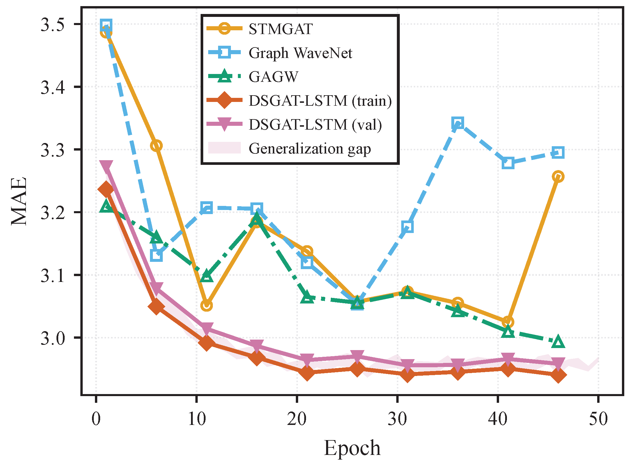Figure 2 further illustrates the optimization behavior during training: the aggregated MAE decreases steadily and the generalization gap remains small after convergence, indicating stable learning under non-stationary demand. The relative ordering of the compared methods along the learning curves is consistent with the overall comparison, providing an intuitive view of how the proposed model reaches a better solution.

Graph-based models further reduce errors by exploiting inter-spot dependence. STGCN and DCRNN outperform purely temporal backbones, and adaptive-graph methods (Graph WaveNet and AGCRN) provide additional gains, suggesting that scenic-spot interactions change over time and are not fully represented by a fixed topology. Overall, DSGAT-LSTM achieves the best performance with MAE/RMSE of 0.171/0.256 and $R^2$ of 0.820, improving over the strongest baseline AGCRN (0.180/0.265, $R^2$ 0.803). These results indicate that jointly integrating social sensing with dynamic spatio-temporal graph learning yields more accurate and reliable one-step predictions.

Beyond accuracy, Table 2 also reports efficiency indicators to substantiate the “lightweight” claim. Compared with strong adaptive-graph baselines, DSGAT-LSTM uses fewer trainable parameters (0.74 M vs. 1.88 M for AGCRN and 2.10 M for GWN) and achieves lower inference cost per one-step prediction (2.2 ms latency and 240 MB peak memory), while maintaining the best forecasting accuracy. Compared with representative dynamic-graph baselines, DSGAT-LSTM remains markedly more efficient, as EvolveGCN and STGODE typically require additional modules to evolve graph representations over time (e.g., recurrent weight evolution or ODE-based integration), leading to larger computation and memory footprints, whereas our approach updates a sparse Top-K adjacency and performs only a single edge-aware graph-attention aggregation per step.

This efficiency mainly comes from the compact design: we perform one sparse graph-attention aggregation on a Top-K neighborhood ($K=5$) and then apply a lightweight LSTM temporal encoder on a short input window ($L=14$), avoiding deep spatio-temporal convolution stacks or heavy dynamic graph generators. We also note that review texts are encoded offline to obtain daily social sensing features $s_i\left(t\right)$ and ${\mathbf{u}}_i\left(t\right)$; therefore, the online forecasting stage operates only on daily aggregated features, which is favorable for practical deployment in operational monitoring scenarios.

To verify that the improvements are not tied to a specific temporal backbone or initialization choice,

Table 3. Backbone/initialization variants of DSGAT-LSTM (daily 1-step). “Mix” denotes mixed $A\left(t\right)$; “G” and “P” denote geo-only prior and corr-only interaction, respectively.

Variant	MAE ↓	RMSE ↓	${\mathit{R}}^2$ ↑
LSTM + Mix + RoBERTa [37]	0.171	0.256	0.820
LSTM + Mix + BERT [38]	0.174	0.260	0.815
GRU + Mix [39]	0.173	0.259	0.816
TCN + Mix [36]	0.176	0.262	0.812
LSTM + G only	0.175	0.261	0.813
LSTM + P only	0.178	0.265	0.807

summarizes backbone and initialization variants of DSGAT-LSTM. Replacing the LSTM with GRU or TCN yields slightly degraded accuracy, and using BERT initialization for the sentiment encoder performs worse than RoBERTa, but the performance remains consistently competitive. This suggests that the core gain comes from the proposed sensing and graph fusion rather than from a particular backbone choice.

We also examine how the source of adjacency affects results. Initializing the dynamic adjacency with a single component weakens the results compared with the mixed setting. The geo-only prior G captures stable geographic proximity but misses short-term coupling changes reflected by recent demand fluctuations. The corr-only interaction $P\left(t\right)$ captures short-term dependence but can be noisy under regime shifts and does not enforce geographic constraints. The mixed construction balances these effects and yields the best overall accuracy.

5.3. Robustness Under Peaks and Shocks

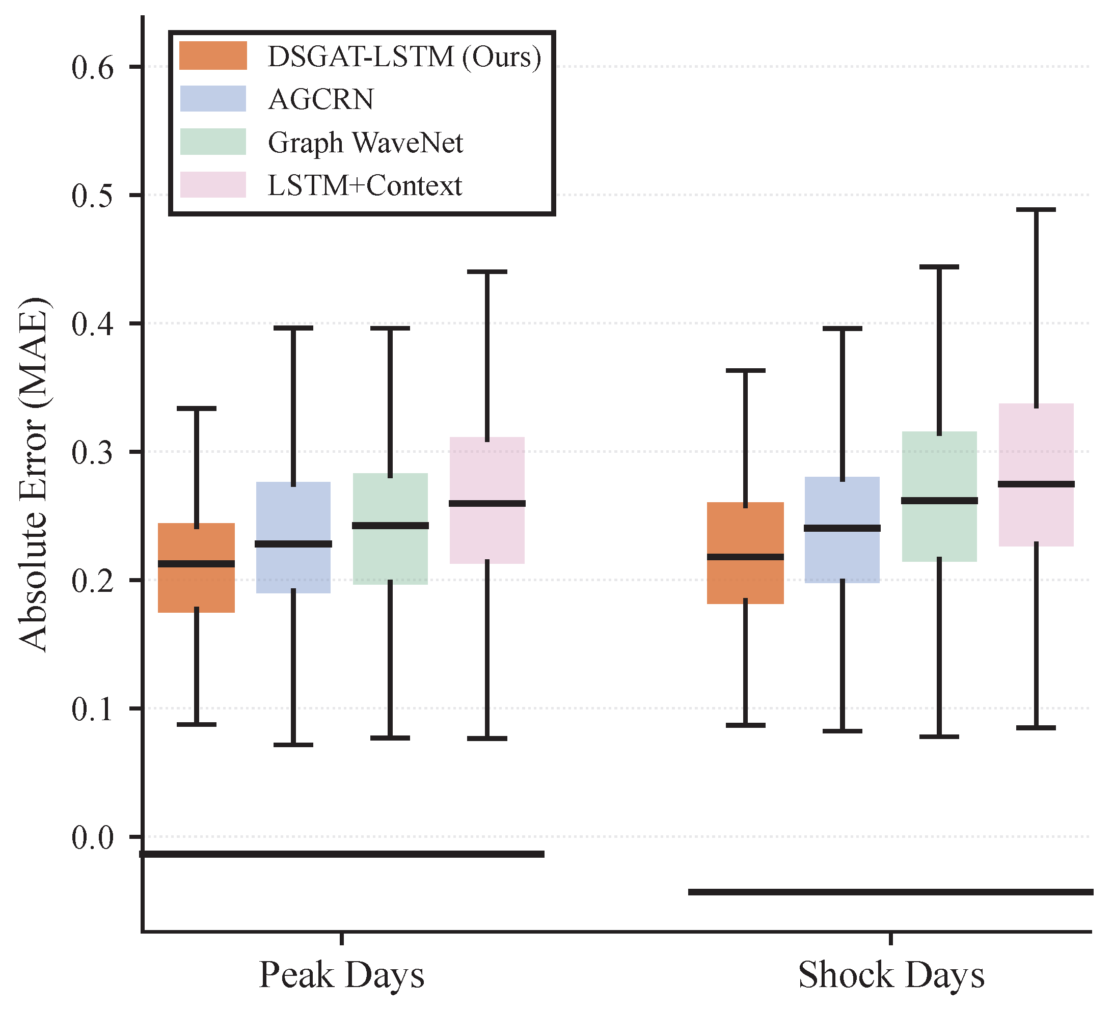
Beyond average accuracy, operational monitoring requires robust performance during extreme periods, where demand exhibits sharp surges or abrupt changes. We therefore evaluate robustness on two challenging subsets constructed from the test set. The Peak subset corresponds to high-demand days defined by the upper quantile of visitor volume. The Shock subset corresponds to days with large day-to-day variations, defined by the upper quantile of $|\Delta y|$, where $\Delta y_i\left(t\right)=y_i\left(t\right)-y_i(t-1)$. For each subset, we compute per-sample absolute forecasting errors and visualize their distributions using boxplots, which reflect the median, dispersion, and outliers.

Figure 3 shows that DSGAT-LSTM achieves lower medians and tighter error spreads than representative baselines on both subsets. The advantage is particularly evident during shocks, where competing methods exhibit larger variance and more high-error outliers. In contrast, DSGAT-LSTM maintains a concentrated error distribution, indicating stronger generalization under rapid regime changes. This robustness is aligned with the design of our framework. Holiday and weather context helps anticipate systematic surges, review-derived social sensing signals capture perception-driven fluctuations, and the daily updated dynamic adjacency adapts inter-spot relations when travel patterns change. Overall, the peak and shock analysis corroborates that DSGAT-LSTM improves both average performance and reliability during operationally critical periods.

5.4. Ablation Study

We conduct an ablation study to quantify the contribution of the key components in DSGAT-LSTM, including dynamic adjacency learning, review-derived social sensing, and delay-aware review alignment.

Table 4. Ablation study of key components (daily 1-step). “Ctx” denotes holiday + weather context. “Gate controls” keep the same gating module but remove informative sentiment input to control for model capacity.

Variant	MAE ↓	RMSE ↓	${\mathit{R}}^2$ ↑
Base (Demand + Ctx)	0.198	0.287	0.771
+ Dynamic adjacency $A\left(t\right)$	0.185	0.270	0.797
+ Sentiment $s_i\left(t\right)$	0.178	0.263	0.808
+ User representation ${\mathbf{u}}_i\left(t\right)$	0.174	0.259	0.815
Full: + Delay-aware alignment	0.171	0.256	0.820
Capacity-matched gate controls (same gate, non-informative input)
Gate with shuffled $s_i\left(t\right)$	0.176	0.262	0.812
Gate with constant/learnable scalar	0.178	0.264	0.807

summarizes a step-by-step augmentation starting from a base setting that uses only demand and exogenous context (holiday + weather).

Adding the daily updated dynamic adjacency $A\left(t\right)$ yields a clear improvement (MAE drops from 0.198 to 0.185), indicating that time-varying inter-spot dependencies provide complementary predictive cues beyond purely temporal patterns and external drivers. Incorporating social sensing further boosts performance: introducing the daily sentiment indicator $s_i\left(t\right)$ reduces MAE to 0.178, and adding the compact review representation ${\mathbf{u}}_i\left(t\right)$ provides an additional gain (MAE 0.174). Finally, enabling delay-aware alignment achieves the best results (MAE/RMSE 0.171/0.256, $R^2$ 0.820), suggesting that correcting review posting delays reduces temporal mismatch and strengthens the effective coupling between social signals and on-site demand.

We emphasize that these results should be interpreted as predictive utility rather than strict causal attribution, since the study is based on observational data. To address the concern that the gains from the sentiment-based social gate might stem from increased model capacity rather than genuinely informative signals, we additionally include capacity-matched controls. Specifically, we keep the same gating module but replace the sentiment input with a time-shuffled sequence (breaking temporal alignment while preserving marginal statistics) or a constant/learnable scalar (preserving parameterization but removing social information). As shown in Table 4, both controls lead to noticeably worse performance than using the true aligned sentiment, and they fall close to the variant without sentiment-based social information. This indicates that the observed improvements are not explained solely by adding parameters; they rely on the informative and temporally aligned social signal.

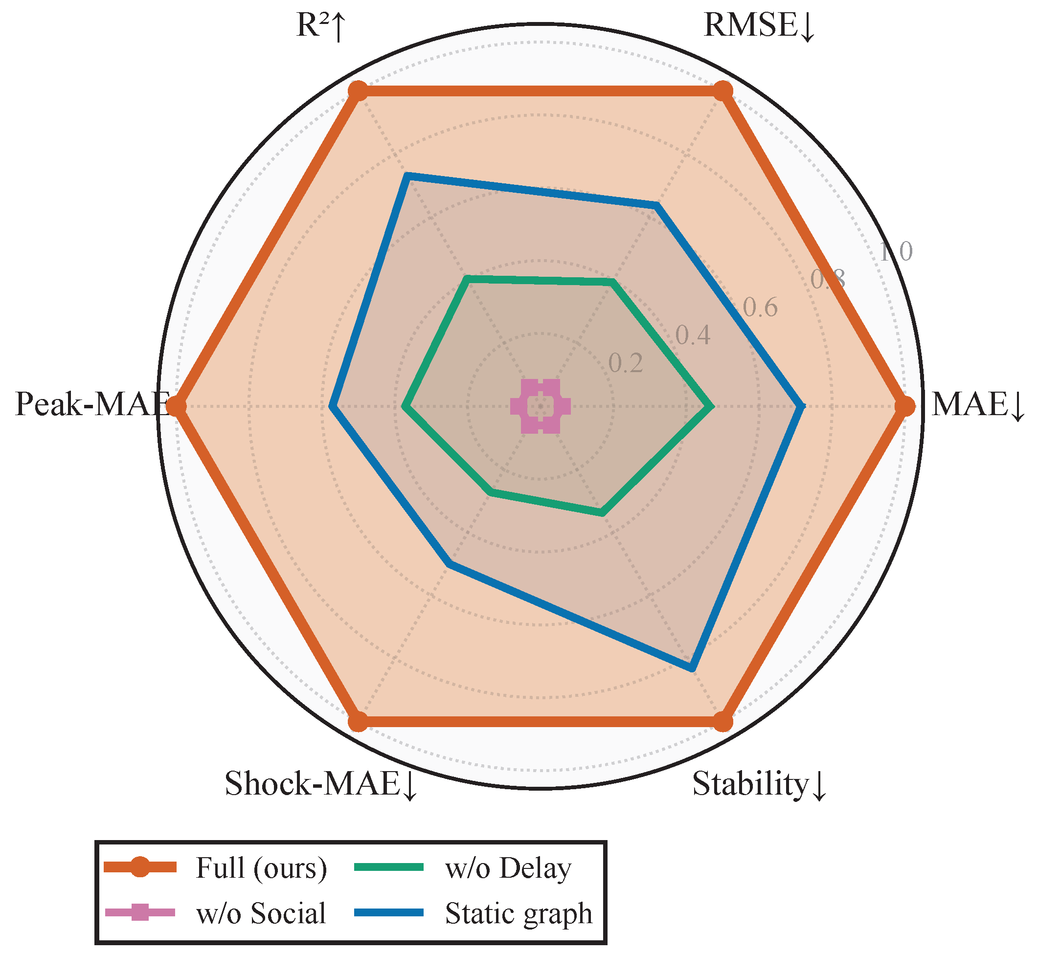
To examine robustness beyond average metrics, Figure 4 provides a radar-chart comparison over multiple normalized criteria, including overall accuracy, peak/shock errors, and stability. The full model consistently attains the largest normalized area. Removing social sensing or delay alignment leads to notable degradations, especially on shock-related criteria. Using a static graph partially preserves stability but sacrifices accuracy and peak/shock robustness compared with the dynamic-graph setting, highlighting the value of adapting inter-spot relations over time.

5.5. Qualitative Analysis and Interpretability

To further interpret the proposed framework beyond aggregate metrics, we provide two complementary visual analyses focusing on (i) the learned dynamic inter-spot relations and (ii) the temporal contribution of social sensing.

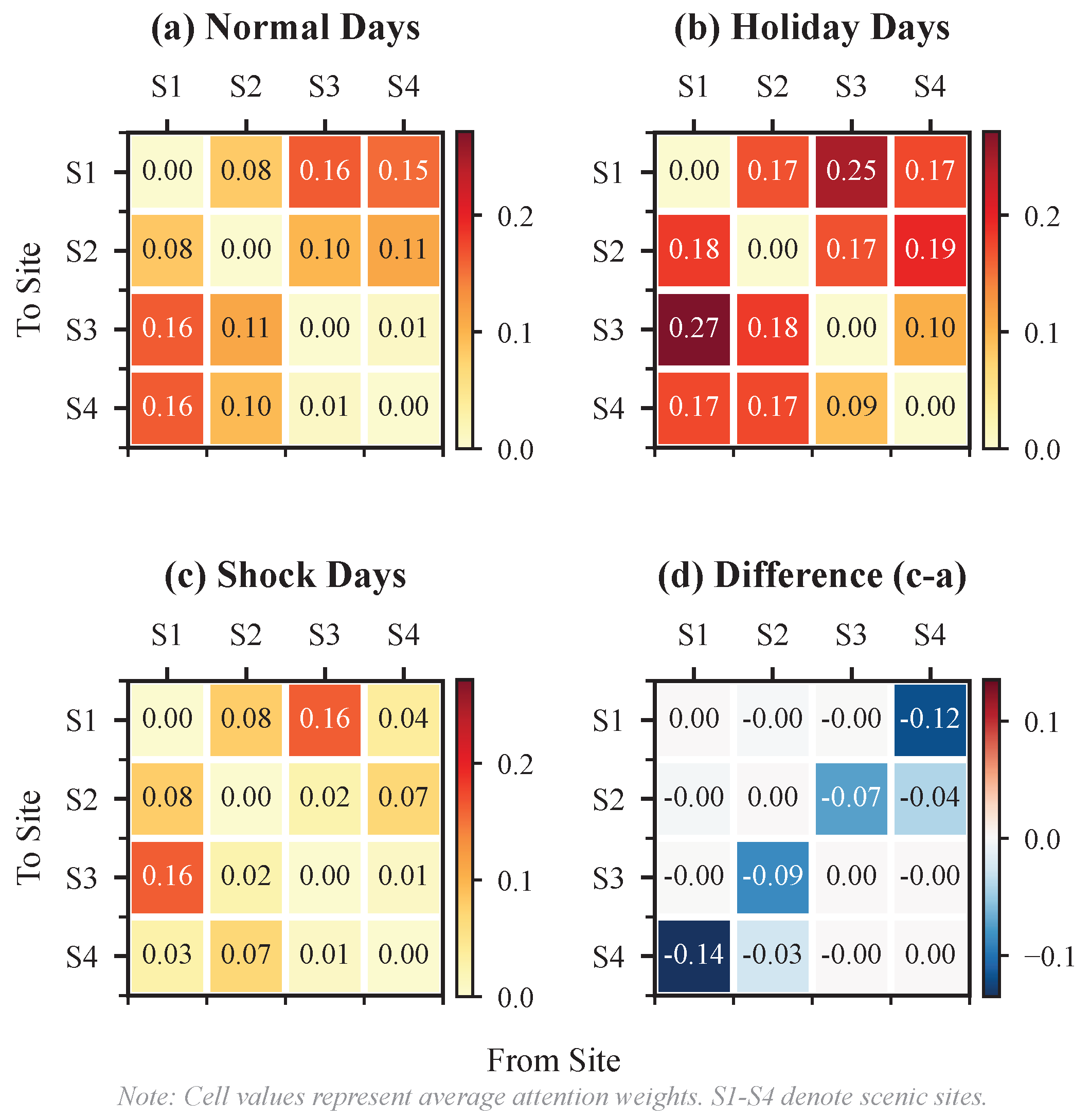
Figure 5 visualizes the learned dynamic adjacency among four representative scenic spots under different regimes. Compared with normal days (Figure 5a), the adjacency during holiday/peak periods (Figure 5b) exhibits generally strengthened cross-site connections, which is consistent with intensified inter-spot coupling induced by itineraries and diversion effects. Shock days (Figure 5c) present a different interaction pattern, and the difference map (Figure 5d, shock minus normal) highlights where connections are amplified or attenuated, indicating that the inferred topology adapts to abrupt changes rather than remaining static.

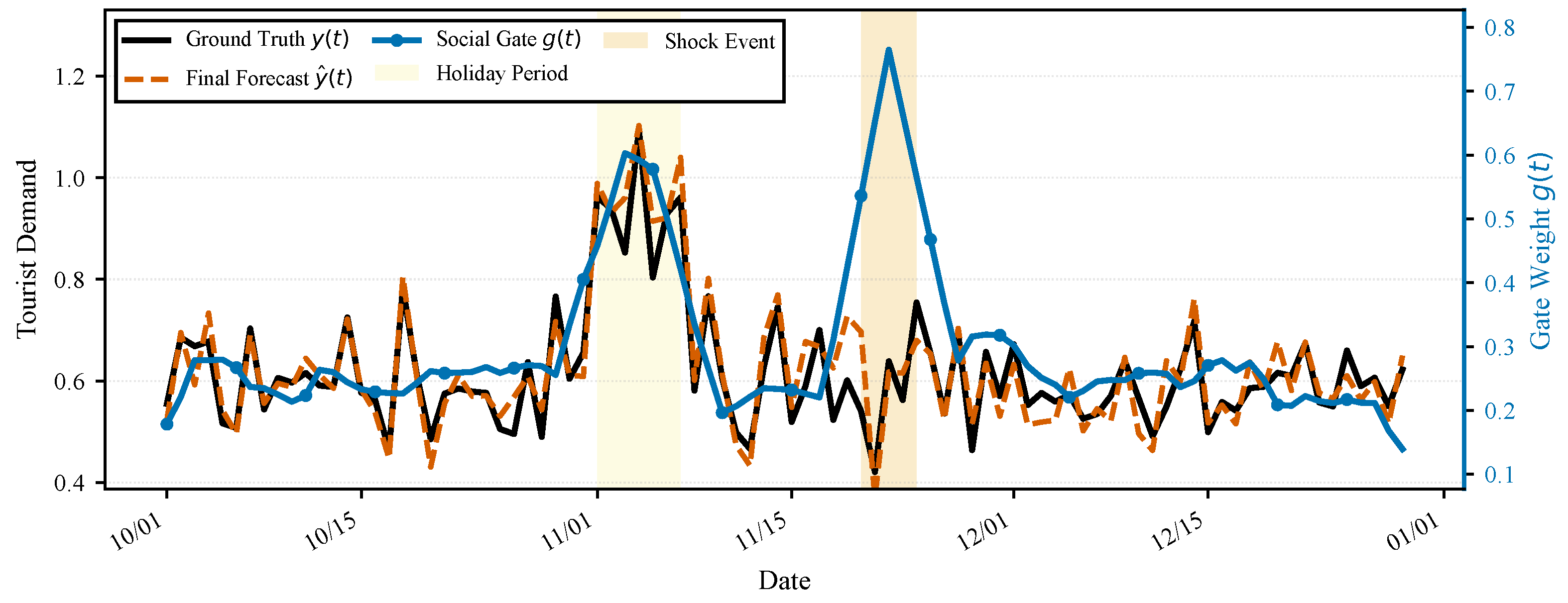
Figure 6 illustrates when social sensing becomes influential by plotting the ground-truth demand $y\left(t\right)$ and prediction $\widehat{y}\left(t\right)$ together with the learned social gate weight for a representative scenic spot. The gate remains relatively stable during routine periods, while it increases around holiday peaks and shock windows (shaded regions), implying that the model allocates more emphasis to review-derived signals when demand becomes more volatile and harder to extrapolate from historical flow alone. Meanwhile, the prediction curve tracks the ground truth more closely during these challenging periods, suggesting that sentiment and semantic information provide corrective cues for short-horizon forecasting.

5.6. Sensitivity Analysis

To further examine the robustness of DSGAT-LSTM to hyperparameter choices, we conduct a one-factor-at-a-time sensitivity analysis. Unless otherwise stated, we use the default configuration described in the experimental setup (and the dataset/protocol summarized in Table 1). For each trial, we vary one key hyperparameter while keeping all others unchanged, and report the resulting MAE/RMSE/$R^2$ on the same evaluation split.

Table 5. One-factor-at-a-time sensitivity analysis of key hyperparameters (daily 1-step).

Setting	MAE ↓	RMSE ↓	${\mathit{R}}^2$ ↑
Input window length L (days)
$L=7$	0.176	0.262	0.812
$L=14$	0.171	0.256	0.820
$L=21$	0.173	0.259	0.816
Graph window length $L_g$ (days)
$L_g=7$	0.174	0.260	0.815
$L_g=14$	0.171	0.256	0.820
$L_g=21$	0.172	0.258	0.818
Neighborhood size K (dynamic graph)
$K=3$	0.173	0.258	0.817
$K=5$	0.171	0.256	0.820
$K=7$	0.175	0.261	0.814
Max review lag $\Delta$ (days)
$\Delta =1$	0.173	0.258	0.817
$\Delta =3$	0.171	0.256	0.820
$\Delta =7$	0.174	0.260	0.815
Review recency decay ${\lambda }_r$
${\lambda }_r=0.2$	0.173	0.259	0.816
${\lambda }_r=0.5$	0.171	0.256	0.820
${\lambda }_r=1.0$	0.174	0.260	0.815
Adjacency mixing $\eta$
$\eta =0.3$	0.172	0.257	0.818
$\eta =0.5$	0.171	0.256	0.820
$\eta =0.7$	0.173	0.258	0.817

indicates that the performance remains stable within a reasonable range, and the default setting (e.g., $L=14$, $L_g=14$, $K=5$, $\Delta =3$, ${\lambda }_r=0.5$, $\eta =0.5$) lies near the best-performing region. In particular, a too-short temporal window (e.g., $L=7$) tends to under-capture weekly patterns, while overly dense neighborhoods (e.g., $K=7$) may introduce noisy dependencies, leading to slightly degraded accuracy.

We also observe that varying the graph-correlation window length $L_g$ in $\{7,14,21\}$ results in only minor changes in MAE/RMSE/$R^2$, suggesting that the daily updated interaction term is not overly sensitive to this short-window choice. This empirical stability supports using $L_g=14$ as a practical trade-off between responsiveness and variance in operational one-step forecasting. In addition, to reduce potential instability caused by sign-flipping correlations under shocks, we employ a conservative nonnegative truncation when constructing $A\left(t\right)$ (see Section 3.5), while alternative signed or robust dependence estimators can also be considered.

6. Discussion

The proposed framework integrates social sensing and dynamic graph learning under explicit consideration of symmetry properties that are essential for geospatial forecasting systems. At its core, the graph attention mechanism preserves permutation equivariance: predictions remain invariant to arbitrary reordering of scenic-spot indices, depending solely on the relative configuration of node features and adjacency structure. This foundational symmetry is maintained throughout the spatio-temporal aggregation process.

Beyond basic permutation invariance, our dynamic adjacency construction introduces geospatial symmetry constraints through the mixed formulation $\mathbf{A}\left(t\right)=\eta \mathbf{G}+(1-\eta )\mathbf{P}\left(t\right)$. The geographic prior $\mathbf{G}$, derived from pairwise great-circle distances, embodies two intrinsic symmetries of physical space: distance symmetry ($d_{ij}=d_{ji}$) and translation/rotation invariance. By anchoring the dynamic graph to this prior, we ensure that learned inter-spot interactions respect the underlying spatial reality even when short-term demand correlations become noisy or sparse. This contrasts with purely data-driven dynamic graph approaches that may generate topologies violating basic geographic constraints during regime shifts.

The time-varying component $\mathbf{P}\left(t\right)$, computed from recent demand co-fluctuations, adapts the graph structure to evolving travel patterns while maintaining symmetry through correlation symmetrization and nonnegative truncation. This design provides a form of temporal stability: similar demand patterns over sliding windows yield similar adjacency structures, creating a predictable evolution of graph connectivity that aligns with observed behavioral regularities.

Regarding the sentiment-guided modulation, the gating mechanism $g_i\left(t\right)=\sigma ({\omega }_g{s}_i\left(t\right)+b_g)$ preserves parameter-sharing symmetry while allowing node-specific responses to social sensing signals. Specifically, the same transformation applies to all nodes through shared parameters $({\omega }_g,b_g)$, yet the resulting gate values vary per node based on their respective sentiment signals $s_i\left(t\right)$. This design maintains the equivariance property of the graph attention layer while enabling adaptive feature recalibration based on review-derived sentiment. The modulation does not break permutation symmetry because the gating function is applied node-wise with shared parameters, and the sentiment signal $s_i\left(t\right)$ itself is derived from node-specific review aggregations.

These symmetry considerations collectively contribute to the observed robustness under peak and shock conditions. The geographic prior provides a stable baseline that prevents the graph from deviating arbitrarily from physically plausible connections, the correlation-based update captures genuine temporal dependencies, and the sentiment modulation adjusts feature importance without disrupting the underlying graph symmetry. This balanced approach allows the model to adapt to changing patterns while retaining the structural consistency needed for reliable forecasting in real-world tourism systems.

The nonnegative truncation in our dynamic adjacency construction enforces a homophilic graph structure, which may not explicitly capture competitive relationships (e.g., substitution effects between distant attractions). While this design choice ensures numerical stability in attention aggregation and aligns with geographic proximity priors, it limits the model’s ability to represent heterophilic structures [40]. Future work could explore signed graph formulations or heterophilic GNN architectures that maintain separate channels for positive and negative correlations, potentially better capturing both cooperative and competitive dynamics in tourism systems.

7. Conclusions

This work addresses daily one-step scenic-spot visitor demand forecasting in a geospatial social and physical sensing setting by jointly leveraging gate/turnstile flow observations, holiday and weather context, and online reviews as social sensing signals. We proposed a delay-aware alignment that converts asynchronously posted reviews into temporally consistent daily sentiment and semantic representations, and we modeled evolving inter-spot interactions through a daily updated dynamic adjacency that combines a coordinate-derived geospatial proximity prior with short-term dependence patterns inferred from recent demand dynamics. Building on these components, we developed DSGAT-LSTM, which integrates sentiment-guided feature modulation, edge-aware dynamic graph attention, and temporal encoding to improve forecasting reliability under non-stationary demand. Experimental results on a multi-year real-world dataset indicate that the proposed framework consistently outperforms representative temporal and spatio-temporal baselines and remains more stable during peak-demand and shock periods, while ablation analyses confirm that the gains come from the complementary contributions of social sensing, delay handling, and dynamic graph modeling. Our current evaluation is limited to a single-region dataset due to the availability of sensing-derived demand labels. Future work will extend the study to multi-region and cross-country benchmarks when comparable demand proxies and review streams can be obtained, to further assess transferability across tourism infrastructures.

References

- Ackermann, L.; Baum, C.; Khalil, S.I.; Litvin, A.; Nicklas, D. Privacy-aware publication of Wi-Fi sensor data for crowd monitoring and tourism analytics. In Proceedings of the 1st ACM SIGSPATIAL International Workshop on Geo-Privacy and Data Utility for Smart Societies, Hamburg, Germany, 13–16 November 2023; pp. 20–23. [Google Scholar]
- Li, H.; Gao, H.; Song, H. Tourism forecasting with granular sentiment analysis. Ann. Tour. Res. 2023, 103, 103667. [Google Scholar] [CrossRef] [Scilit]
- Ke, Z.; Shen, J.; Zhao, X.; Fu, X.; Wang, Y.; Li, Z.; Mu, H. A stable technical feature with GRU-CNN-GA fusion. Appl. Soft Comput. 2025, 187, 114302. [Google Scholar] [CrossRef] [Scilit]
- Ma, S.; Li, H.; Hu, M.; Yang, H.; Gan, R. Tourism demand forecasting based on user-generated images on OTA platforms. Curr. Issues Tour. 2024, 27, 1814–1833. [Google Scholar] [CrossRef] [Scilit]
- Ke, Z.; Cao, Y.; Chen, Z.; Yin, Y.; He, S.; Cheng, Y. Early warning of cryptocurrency reversal risks via multi-source data. Financ. Res. Lett. 2025, 85, 107890. [Google Scholar] [CrossRef] [Scilit]
- Li, Y.; Yu, R.; Shahabi, C.; Liu, Y. Diffusion convolutional recurrent neural network: Data-driven traffic forecasting. In Proceedings of the International Conference on Learning Representations, Vancouver, BC, Canada, 30 April–3 May 2018. [Google Scholar]
- Yu, B.; Yin, H.; Zhu, Z. Spatio-temporal graph convolutional networks: A deep learning framework for traffic forecasting. In Proceedings of the 27th International Joint Conference on Artificial Intelligence, Stockholm, Sweden, 13–19 July 2018; pp. 3634–3640. [Google Scholar]
- Guo, S.; Lin, Y.; Feng, N.; Song, C.; Wan, H. Attention-based spatial-temporal graph convolutional networks for traffic flow forecasting. Proc. AAAI Conf. Artif. Intell. 2019, 33, 922–929. [Google Scholar] [CrossRef] [Scilit]
- Hou, Y.; Zhao, S.; Xia, X.; Liwang, M.; Li, Z.; Xu, N.; Quek, T.Q. FedC-DAC: A Federated Clustering with Dynamic Aggregation and Calibration Method for SAR Image Target Recognition. IEEE J. Select. Top. Appl. Earth Obs. Remote Sens. 2025, 19, 3726–3745. [Google Scholar] [CrossRef] [Scilit]
- Jin, G.; Liang, Y.; Fang, Y.; Shao, Z.; Huang, J.; Zhang, J.; Zheng, Y. Spatio-temporal graph neural networks for predictive learning in urban computing: A survey. IEEE Trans. Knowl. Data Eng. 2024, 36, 5388–5408. [Google Scholar] [CrossRef] [Scilit]
- Sahili, Z.A.; Awad, M. Spatio-temporal graph neural networks: A survey. arXiv 2023, arXiv:2301.10569. [Google Scholar] [CrossRef] [Scilit]
- He, Q.; Qu, C. Modular Landfill Remediation for AI Grid Resilience. arXiv 2025, arXiv:2512.19202. [Google Scholar] [CrossRef] [Scilit]
- Sánchez, P.; Bellogín, A.; Jorro-Aragoneses, J.L. Context Trails: A dataset to study contextual and route recommendation. In Proceedings of the 19th ACM Conference on Recommender Systems, Prague, Czech Republic, 22–26 September 2025; pp. 716–725. [Google Scholar]
- Wongso, W.; Xue, H.; Salim, F.D. Massive-STEPS: Massive semantic trajectories for understanding POI check-ins: Dataset and benchmarks. arXiv 2025, arXiv:2505.11239. [Google Scholar]
- He, Q. Location-Robust Cost-Preserving Blended Pricing for Multi-Campus AI Data Centers. arXiv 2025, arXiv:2512.14197. [Google Scholar]
- Lim, B.; Arik, S.Ö.; Loeff, N.; Pfister, T. Temporal fusion transformers for interpretable multi-horizon time series forecasting. Int. J. Forecast. 2021, 37, 1748–1764. [Google Scholar] [CrossRef] [Scilit]
- Hanawa, K.; Terabe, S.; Yaginuma, H.; Tanaka, K. Recommendation system for tourist attractions based on Wi-Fi packet sensor data. Transp. Res. Rec. 2023, 2677, 333–342. [Google Scholar] [CrossRef] [Scilit]
- He, Q. A unified metric architecture for ai infrastructure: A cross-layer taxonomy integrating performance, efficiency, and cost. arXiv 2025, arXiv:2511.21772. [Google Scholar]
- Zhang, P.; Li, X.; Yu, L.; Zhang, Z.; Dunkin, F.; Liu, H.; Li, Z. Boosting Learning Efficiency in Few-Shot Tasks With Layer-Adaptive PID Control. IEEE Trans. Pattern Anal. Mach. Intell. 2026. [Google Scholar] [CrossRef] [Scilit]
- Shen, Q.; Zhang, J. MFTFormer: Meteorological-Frequency-Temporal Transformer with Block-Aligned Fusion for Traffic Flow Prediction. Res. Sq. 2026, preprint. [Google Scholar] [CrossRef] [Scilit]
- Wu, Z.; Pan, S.; Long, G.; Jiang, J.; Zhang, C. Graph WaveNet for deep spatial-temporal graph modeling. In Proceedings of the 28th International Joint Conference on Artificial Intelligence, Macao, China, 10–16 August 2019; pp. 1907–1913. [Google Scholar]
- Bai, L.; Yao, L.; Li, C.; Wang, X.; Wang, C. Adaptive graph convolutional recurrent network for traffic forecasting. In Advances in Neural Information Processing Systems; NeurIPS Foundation: Red Hook, NY, USA, 2020; Volume 33, pp. 17804–17815. [Google Scholar]
- Wu, Z.; Pan, S.; Long, G.; Jiang, J.; Chang, X.; Zhang, C. Connecting the dots: Multivariate time series forecasting with graph neural networks. In Proceedings of the 26th ACM SIGKDD International Conference on Knowledge Discovery & Data Mining, Virtual Event, 6–10 July 2020; pp. 753–763. [Google Scholar]
- Pareja, A.; Domeniconi, G.; Chen, J.; Ma, T.; Suzumura, T.; Kanezashi, H.; Kaler, T.; Schardl, T.B.; Leiserson, C.E. EvolveGCN: Evolving graph convolutional networks for dynamic graphs. In Proceedings of the 34th AAAI Conference on Artificial Intelligence, New York, NY, USA, 7–12 February 2020; pp. 5363–5370. [Google Scholar]
- Fang, Z.; Long, Q.; Song, G.; Xie, K. Spatial-temporal graph ODE networks for traffic flow forecasting. In Proceedings of the 27th ACM SIGKDD International Conference on Knowledge Discovery & Data Mining, Virtual Event, 14–18 August 2021; pp. 364–373. [Google Scholar]
- Qiu, Y.; Yin, J.; Zhang, T.; Du, Y.; Zhang, B. Spatiotemporal dynamic analysis of A-level scenic spots in Guizhou Province, China. ISPRS Int. J. Geo-Inf. 2021, 10, 568. [Google Scholar] [CrossRef] [Scilit]
- Wu, X.; Chen, C. Spatial distribution and accessibility of high-level scenic spots in Inner Mongolia. Sustainability 2022, 14, 7329. [Google Scholar] [CrossRef] [Scilit]
- He, Q.; Qu, C. Waste-to-Energy-Coupled AI Data Centers: Cooling Efficiency and Grid Resilience. arXiv 2025, arXiv:2512.24683. [Google Scholar]
- Hou, Y.; Yu, B.; Yang, Z.; Wang, J.; Xiang, W.; Wu, D.; Liwang, M.; Xia, X.; Li, Z.; Tian, Y.; et al. Privacy-Preserving Federated SAR Image Target Recognition with Adaptive Resource Management in Space-Air-Ground Integrated Networks. Pattern Recognit. 2026, 177, 113253. [Google Scholar] [CrossRef] [Scilit]
- Yao, Z.; Zhu, Q. A Two-Stage Wiener Process-Based Method for Bearing Remaining Useful Life Prediction Considering Measurement Uncertainty. Meas. Sci. Technol. 2026, 37, 066203. [Google Scholar] [CrossRef] [Scilit]
- Yao, S.; Guan, R.; Wu, Z.; Ni, Y.; Huang, Z.; Liu, R.; Yue, Y. Waterscenes: A multi-task 4d radar-camera fusion dataset and benchmarks for autonomous driving on water surfaces. IEEE Trans. Intell. Transp. Syst. 2024, 25, 16584–16598. [Google Scholar] [CrossRef] [Scilit]
- Shen, Q.; Zhang, J. AI-Enhanced Disaster Risk Prediction with Explainable SHAP Analysis: A Multi-Class Classification Approach Using XGBoost. Res. Sq. 2025, preprint. [Google Scholar] [CrossRef] [Scilit]
- Box, G.E.P.; Jenkins, G.M.; Reinsel, G.C.; Ljung, G.M. Time Series Analysis: Forecasting and Control, 5th ed.; Wiley: Hoboken, NJ, USA, 2015. [Google Scholar]
- Chen, T.; Guestrin, C. XGBoost: A scalable tree boosting system. In Proceedings of the 22nd ACM SIGKDD International Conference on Knowledge Discovery and Data Mining, San Francisco, CA, USA, 13–17 August 2016; pp. 785–794. [Google Scholar]
- Hochreiter, S.; Schmidhuber, J. Long short-term memory. Neural Comput. 1997, 9, 1735–1780. [Google Scholar] [CrossRef] [Scilit] [PubMed]
- Bai, S.; Kolter, J.Z.; Koltun, V. An empirical evaluation of generic convolutional and recurrent networks for sequence modeling. arXiv 2018, arXiv:1803.01271. [Google Scholar] [CrossRef] [Scilit]
- Liu, Y.; Ott, M.; Goyal, N.; Du, J.; Joshi, M.; Chen, D.; Levy, O.; Lewis, M.; Zettlemoyer, L.; Stoyanov, V. RoBERTa: A robustly optimized BERT pretraining approach. arXiv 2019, arXiv:1907.11692. [Google Scholar]
- Devlin, J.; Chang, M.-W.; Lee, K.; Toutanova, K. BERT: Pre-training of deep bidirectional transformers for language understanding. In Proceedings of the 2019 Conference of the North American Chapter of the Association for Computational Linguistics: Human Language Technologies, Minneapolis, MN, USA, 2–7 June 2019; pp. 4171–4186. [Google Scholar]
- Cho, K.; van Merriënboer, B.; Bahdanau, D.; Bengio, Y. On the properties of neural machine translation: Encoder–decoder approaches. In Proceedings of the Workshop on Syntax, Semantics and Structure in Statistical Translation, Doha, Qatar, 25 October 2014; pp. 103–111. [Google Scholar]
- Luan, S.; Hua, C.; Xu, M.; Lu, Q.; Zhu, J.; Chang, X.; Fu, J.; Leskovec, J.; Precup, D. When do graph neural networks help with node classification? Investigating the homophily principle on node distinguishability. In Advances in Neural Information Processing Systems; NeurIPS Foundation: Red Hook, NY, USA, 2023; Volume 36, pp. 28748–28760. [Google Scholar]
Figure 1.
Conceptual overview: fusing on-site sensing, social sensing, and context on a daily updated graph for one-step scenic-spot demand forecasting. Here, is daily visitor demand; is aligned daily sentiment; is the aggregated daily review embedding; and denotes exogenous context (holiday and weather).
Figure 2.
Training dynamics (MAE vs. epoch) of DSGAT-LSTM on the scenic-spot dataset. MAE is reported as an aggregated error over all scenic spots to better visualize convergence and the generalization gap; the corresponding per-spot averaged MAE is used for quantitative reporting.
Figure 3.
Error distribution under peak and shock conditions. Boxplots show per-sample absolute errors of DSGAT-LSTM and representative baselines on Peak and Shock subsets, highlighting improved robustness through lower medians and tighter spreads.
Figure 4.
Radar-chart comparison of ablation variants across multiple normalized criteria, including overall accuracy, peak/shock errors, and stability.
Figure 5.
Visualization of the learned dynamic adjacency for four representative scenic spots. (a) Normal days, (b) holiday/peak days, (c) shock days, and (d) difference map (shock minus normal).
Figure 6.
Temporal visualization of social-sensing gating. The ground-truth demand , the final model output (i.e., the predicted demand after social-gate fusion), and the learned social gate weight are shown for a representative scenic spot. Shaded regions indicate holiday/peak and shock periods.