Abstract
The identification of topological phases in disordered systems is a significant field in condensed matter physics, where disorder breaks translational symmetry and invalidates conventional topological invariants defined in momentum space. Currently, machine learning offers promising alternatives in the identification of topological phases. In this work, by regarding the population dynamics as input data, we used feedforward neural networks (FNNs), vanilla recurrent neural networks (RNNs), and long short-term memory (LSTM) networks to identify the topology in the Su–Schrieffer–Heeger (SSH) model and the disordered SSH model, respectively. We also compared the identification capabilities of different neural networks using different input data. Our results show that FNN has the lowest training cost and a relatively high prediction accuracy. However, when increasing the time length and reducing the number of time points, vanilla RNN has higher prediction accuracy. Furthermore, we develop an interactive web-based tool, enabling real-time topological phase prediction based on user-specified parameters. This study not only lays the foundation for researchers to identify topology by using population dynamics as the input data of neural networks but also provides an accessible platform to support data-driven exploration of complex quantum phases.
1. Introduction
Topological states of matter [1,2,3,4,5,6,7,8,9,10,11], as a frontier in condensed matter physics, are characterized by global topological invariants such as Chern numbers [2] and winding numbers [1]. Traditionally, the computation of these topological invariants relies on Bloch wave functions in momentum space, which requires translational symmetry in the system. However, disorder is inevitable in real materials or synthetic systems and can even induce novel topological phase transitions [12,13,14,15,16,17,18,19]. Such disordered topological systems cannot be effectively characterized by conventional momentum-space approaches, as disorder breaks translational symmetry and invalidates Bloch theory. Although real-space topological numbers have been proposed as an alternative [16], their construction and computation still depend on handcrafted indicators, making them difficult to generalize to complex or non-Hermitian systems.
These challenges have motivated increasing interest in machine learning approaches for identifying topological phases and invariants [20,21,22,23,24,25,26,27,28,29,30,31,32,33,34,35,36]. Previous research work has shown that neural networks can identify the winding number from the Hamiltonian in momentum space [24,25] and real space [37], and have successfully carried out topological classification through the population dynamics [38] or Hamiltonian [39] in an unsupervised manner. However, relevant research on identifying the topology of disordered models through population dynamics is still relatively scarce at present.
In this work, we used feedforward neural networks (FNNs), vanilla recurrent neural networks (RNNs), and long short-term memory (LSTM) networks respectively to identify the topology of the Su–Schrieffer–Heeger (SSH) model and the disordered SSH model [40,41,42,43,44]. Instead of using the Hamiltonian or projection operators, we used the experimentally measurable population dynamics as input data. This enables the model to learn topological features directly from real-time evolution. In addition, by changing the input data, we compared the recognition abilities of the three networks under different conditions.
Our results show that when the input data is appropriate, all three networks can accurately identify the topology of two models, and the FNN has the lowest training cost. When the input data changes, the recognition abilities of the three networks will vary. We compared the prediction accuracies of the three networks under different numbers of cells N, time lengths T, numbers of time points , and generation times . Our results lay the foundation for identifying the topology by using the population dynamics as the network input. Finally, to bridge numerical results with practical use, we implement a web-based prediction tool that allows real-time inference of the topological phase from user-specified disorder and hopping parameters [45].
2. Model
In this section, we introduced two one-dimensional topological models: the SSH model and the disordered SSH model. In Section 2.1, taking the one-dimensional SSH model as an example, we introduced the mathematical calculation methods we used: calculating the population dynamics through the Hamiltonian and calculating the topological number through the expectation value of the chiral displacement operator. In Section 2.2, we mainly introduced how disorder is introduced in the disordered SSH model.
2.1. SSH Model
We first introduce a one-dimensional SSH model. As shown in Figure 1a, each unit cell of the model comprises two sublattice sites, A and B. The Hamiltonian of the SSH model is written as
where p represents the intra-cell hopping strength and q denotes the inter-cell hopping strength, are the Pauli matrices, and h.c. denotes the Hermitian conjugate. The creation operator creates a particle in unit cell n on sublattice site A or B, where is the corresponding annihilation operator.
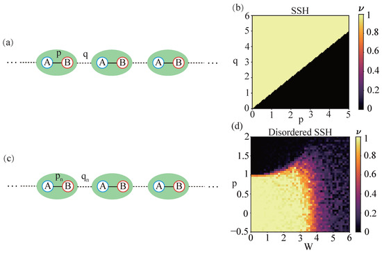
Figure 1.
Model and phase diagram. (a) Schematic diagram of the SSH model. Each unit cell represented by a green background contains two sublattices labeled as A and B. The inter- and intra-cell hopping strengths are denoted by q and p, respectively, and n represents the serial number of the unit cell. (b) Topological phase diagram of the SSH model as a function of inter-cell hopping q and intra-cell hopping p. When , the winding number is 1, and the model is in the topological phase. When , the winding number is 0, and the model is in the trivial phase. (c) Schematic diagram of the disordered SSH model. Similar to (a), the inter- and intra-cell hopping strengths are denoted by and , respectively. The disorder of hopping is introduced by the random numbers and , and represents the disorder strengths. (d) Topological phase diagram of the disordered SSH model as a function of parameter p and disorder strengths W with and .
By solving the Schrödinger equation
we obtain the wave function , where . The initial state is set such that a particle is placed at the A sublattice site of the 0-th unit cell. We take the population dynamics of the system
Following the method in Ref. [16], the expression for calculating the winding number through the population dynamics is written as
where is the expectation value of the chiral displacement operator, is the chiral operator and X is the unit cell operator. The time length T is the maximum duration considered when performing a time average. Under ideal conditions, the phase diagram of the SSH model is shown in Figure 1b. When the intra-cell coupling is less than the inter-cell coupling, the winding number is 1, and the SSH model is in a topologically non-trivial phase. Otherwise, the winding number is 0, and the SSH model is in a topologically trivial phase.
2.2. Disordered SSH Model
Subsequently, we introduce disorder into the SSH model. As shown in Figure 1c, the Hamiltonian of the disordered SSH model is written as
where are the Pauli matrices acting on the sublattice degree of freedom. The parameters and characterize the intra-cell and inter-cell hopping strength, respectively. We define the controlled fluctuations in the hopping terms using parameters:
The disorder is introduced via and , which are independent random numbers uniformly sampled from , and , which are the dimensionless disorder strengths for the inter- and intra-cell hopping, respectively. In this article, we fix the disorder strength to be and .
Same as the SSH model, the initial state is set such that a particle is placed at the A sublattice of the 0-th unit cell and Equations (2) and (3) are used to calculate the population dynamics. The topological phase diagram of the disordered SSH model calculated by population dynamics is shown in Figure 1d. This phase diagram is determined by obtaining the winding number through the expectation value C of the chiral displacement operator. Different from the SSH model, when calculating the winding number in the disordered SSH model, one not only needs to perform a time average on the expectation value C as shown in Equation (4), but also to perform a disorder average.
The parameters of this work are shown in Table 1.

Table 1.
The parameters of this work.
3. Generalization of Training, Validation and Test Data
Before applying a specific neural network, we first generate the training, validation and test data for the neural network. Considering that the winding number can be calculated through population dynamics, we use population dynamics as the input of the neural network to train the network to identify the topology of the model. In this section, we introduce how the training, validation and test data for the neural network in this article are generated.
The number of unit cells N in the model used to calculate the population dynamics is 200. To prevent large errors in the calculated winding number v due to the propagation of population dynamics to the model boundaries, we set the time length and the number of time points . For the SSH model, the input data consist of the population at all lattice sites across 100 time points, with a single input dimension of . For the disordered SSH model, since the dynamics generated each time are different, we set the generation counts to generate 100 sets of independent data, each recording the population at all lattice sites over 100 time points (). These 100 datasets are concatenated along the time dimension to form a single input with a final dimension of 400 × 10,000.
We generated 10,000 independent input data for each model, with 6000 of them used as training data, 2000 of them used as validation data and 2000 of them as test data. The parameter selection ranges for the SSH model and the disordered SSH model correspond to those depicted in Figure 1b,d, respectively. Considering that there is an error in the winding number v calculated using Equation (4), we determine the case of when the winding number is 0, the case of when the winding number is 1, and the case of will be discarded.
In Figure 2, we respectively present the population dynamics used as network input data for the SSH model and the disordered SSH model in the trivial phase and the topological phase. Figure 2(a1,b1) present the population dynamics of the SSH model across sites −50th to 50th under different topological phases. Figure 2(a2,b2) then zoom in on the local dynamics by tracking the evolution of all sites in the 0th cells—namely, site A and site B of the 0th unit cell (, ) over the same time period. The evolution of each site is clearly represented by color-coded curves: red for site A, black for site B. Figure 2(c1–d2) illustrate the same physical quantities in the disordered SSH model.
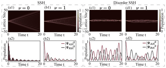
Figure 2.
Temporal evolution of the lattice population. (a1,b1) The figure shows the spatial (from the −50th to the 50th lattice site) and temporal evolution of the lattice population corresponding to different topological numbers in the SSH model. As time goes by, the lattice population gradually spreads from the 0th cell to both sides. (a2,b2) The figure shows the evolution of the lattice population for all sites in the 0th cell of the SSH model, where (red line) and (black line) represent the evolution of the lattice population at site A and B of the 0th cell, respectively. Parameter settings for the SSH model: for ; for . (c1–d2) Same as (a1–b2), but for the disorder SSH model. Different from the SSH model, in the disordered SSH model, the lattice population does not spread to both sides over time, as shown in (c1,d1). This is due to the population localization induced by disorder [46]. (c2,d2) The figure shows the evolution of the lattice population for all sites in the 0th cell of the disordered SSH model. Parameter settings for the disordered SSH model: for and for .
4. Application of Neural Networks
The fundamental function of a neural network is to receive system configuration information (such as images, text, or audio clips) through its input layer, process it layer by layer in hidden layers, and finally generate results at the output layer. Each layer consists of multiple nodes. These nodes are abstract models inspired by biological neurons and serve as the fundamental building blocks of deep learning architectures like feedforward neural networks. Although a single node has a relatively simple structure, combining numerous nodes in a layered manner enables the approximation of arbitrarily complex nonlinear functions.
As information propagates from the input layer to the output layer, the network performs specific nonlinear transformations at each layer, introducing corresponding adjustable parameters (weights and biases). The core objective of network training is to continuously optimize these parameters so that the model’s output gradually approximates the target results. One complete pass through the training set is termed an epoch, and typically multiple epochs are required to achieve stable convergence performance.
In this section, we will introduce the network structures and training methods of the three neural network models we used: FNN, vanilla RNN, and LSTM. We will also compare the network’s predicted output with the average chiral displacement to verify the model’s ability to capture features.
4.1. FNN
We first employ the FNN shown in Figure 3a to identify the topology of the SSH model and the disordered SSH model respectively. For the SSH model, the populations of the model at 100 time points are used as the input of the network. The model we use to calculate the population numbers has 200 unit cells, so the dimension of each sample is . For the disordered SSH model, due to the presence of disorder, the population dynamics calculated each time are different. We need to concatenate the results of 100 calculations, and the dimension of each sample is 400 × 10,000. The data dimensions of both models are compressed to through data preprocessing with average pooling. k is the number of samples. Subsequently, the input data passes through linear layers of 128 and 64 dimensions in sequence to obtain the output of the neural network. After each linear layer, we use the rectified linear unit as the activation function and add a dropout mechanism to randomly discard neurons with a probability of 0.3 to suppress overfitting.
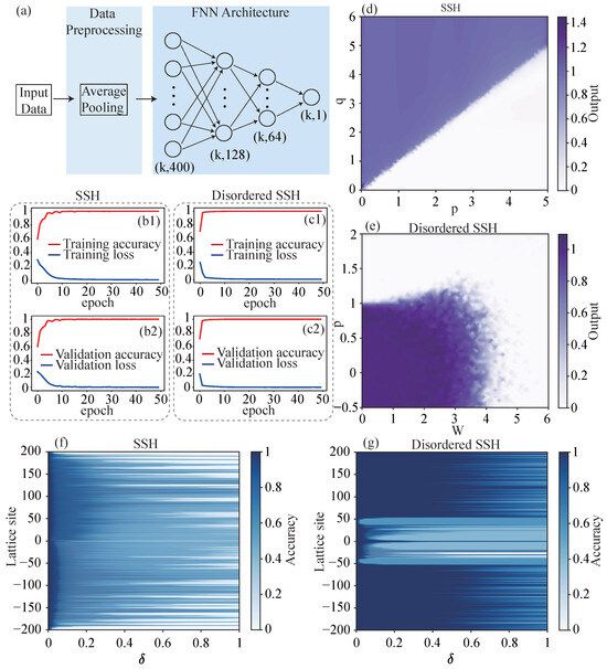
Figure 3.
Training of FNN. (a) Structure diagram of FNN. k is the number of samples. (b1,b2) The accuracy (red line) and loss (blue line) of the (b1) training set and (b2) validation set as functions of epoch when training the FNN identify the topology of the SSH model. (c1,c2) The accuracy (red line) and loss (blue line) of the (c1) training set and (c2) validation set as functions of epoch when training the FNN identify the topology of the disordered SSH model. (d) The output of the trained FNN varies with the parameters p and q of the SSH model. It is similar to the topological phase diagram of the SSH model (Figure 1b), indicating that the FNN can recognize the topology of the SSH model, and the network output is the winding number. (e) The output of the trained FNN varies with the parameters p and W of the disordered SSH model. Similarly, by comparing it with Figure 1d, it can be seen that the FNN can also identify the topology of the disordered SSH model. (f,g) Prediction accuracy of (f) SSH and (g) disordered SSH model for input data with different deviations at different lattice sites. The parameter settings for generating input data are set as , , , and .
During the process of training the network, we divide the training set into batches for training, with a batch size of 64. The mean squared error is used as the loss function for training, and the Adam optimizer is employed. The learning rate is set to , and the remaining parameters are set to their default values. The entire training was carried out for 50 epochs. After each epoch, we recorded the loss and accuracy of the training set and the validation set. The accuracy was calculated by rounding the output data and then comparing it with the winding number. The plotted images are shown in Figure 3(b1–c2). Whether for the SSH model or the disordered SSH model, within a few epochs, the losses of the training set and the validation set are close to 0, and the accuracy is close to 1. After the training, the prediction accuracy of the trained FNN for the test sets of both the SSH model and the disordered SSH model is . This means that the FNN can easily identify the topology of the SSH model and the disordered SSH model, and the network has strong generalization ability. For the input data unseen by the network, such as the validation set and the test set, the prediction accuracy can also reach a very high level.
Figure 3d shows the variation in the FNN output with the parameters p and q of the SSH model. It has an image similar to that in Figure 1b. At the topological boundary of the SSH model, the output of the network also undergoes a sudden change. When , the model output is approximately 1, and when , the model output is approximately 0. Similarly, Figure 3e shows how the output of the network changes with the parameters p and W of the disordered SSH model, and it exhibits a topological boundary similar to that in Figure 1d.
Figure 3f,g show the accuracy of the FNN in identifying the topology of the SSH model and the disordered SSH model for different errors at different lattice sites. The prediction accuracy of each point on the graph is obtained by adding an error to the input data at different lattice sites and then inputting it into the FNN for calculation. For the SSH model, the FNN is more sensitive to the errors at the lattice sites and those of the B sublattice. For the disordered SSH model, since the population is localized in the middle, the FNN is more sensitive to the errors at the middle lattice sites.
4.2. Vanilla RNN
The vanilla RNN we use is shown in Figure 4a. Similar to FNN, we also perform preprocessing of average pooling on the input data. We will also perform data balancing and standardization preprocessing on the data to speed up the convergence during training. Then, we input the data into a bidirectional vanilla RNN layer composed of 400 vanilla RNN units. The hidden dimension size is 64, the nonlinearity is set to , and a dropout mechanism is added to randomly discard neurons with a probability of 0.3. Then, take the output of the last time step of the vanilla RNN layer and input it into a 64-dimensional fully connected layer to obtain the output of the network. Add a rectified linear unit as the activation function and a dropout mechanism after each layer, and set the random discard probability to 0.3.
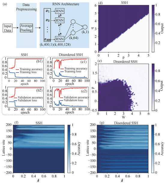
Figure 4.
Training of vanilla RNN. (a) Structure diagram of vanilla RNN. k is the number of samples. (b1,b2) The accuracy (red line) and loss (blue line) of the (b1) training set and (b2) validation set as functions of epoch when training the vanilla RNN identify the topology of the SSH model. (c1,c2) The accuracy (red line) and loss (blue line) of the (c1) training set and (c2) validation set as functions of epoch when training the vanilla RNN identify the topology of the disordered SSH model. (d) The output of the trained vanilla RNN varies with the parameters p and q of the SSH model. (e) The output of the trained vanilla RNN varies with the parameters p and W of the disordered SSH model. (f,g) Prediction accuracy of (f) SSH and (g) disordered SSH model for input data with different deviations at different lattice sites. The parameter settings for generating input data are set as , , , and .
When training the vanilla RNN, use the same batch size, loss function, and optimizer as the FNN, and set the learning rate to . We also performed weight initialization on the network to accelerate convergence, applied orthogonal initialization to the vanilla RNN layer, and applied Kaiming initialization to the fully connected layer. The changes in the loss and accuracy of the training set and validation set with the number of epochs are shown in the Figure 4(b1–c2). After 100 epochs, the prediction accuracy of the vanilla RNN for the training sets and validation sets of both models is close to 1. The prediction accuracy of the trained vanilla RNN for the test sets of the SSH model and the disordered SSH model is and respectively. This indicates that vanilla RNN can also identify the topology of the SSH model and the disordered SSH model. However, compared with FNN, vanilla RNN requires more epochs to achieve the same prediction accuracy.
Figure 4d and Figure 4e respectively show the changes in the vanilla RNN output with the parameters p and q of the SSH model, and with the parameters p and W of the disordered SSH model. Comparing with Figure 1b,d, it can be seen that the output of the vanilla RNN is also the winding number of the model. However, compared with the output of the FNN, the output of the vanilla RNN shows some obviously wrong discrete points at the phase boundary of the disordered SSH model.
Figure 4f,g show the accuracy of the vanilla RNN in identifying the topology of the SSH model and the disordered SSH model for different errors at different lattice sites. For the SSH model, the vanilla RNN is mainly sensitive to errors in the lattice site range of 0–100, but completely insensitive to errors at negative lattice sites. For the disordered SSH model, the vanilla RNN is also only sensitive to the errors at the positive lattice sites. It is not sensitive to the errors at the negative lattice sites.
4.3. LSTM
The LSTM network we use is shown in Figure 5a. Its network structure is similar to that of the vanilla RNN, with the only difference being that the vanilla RNN units are replaced by LSTM units. The training process of the LSTM network is also exactly the same as that of the vanilla RNN and the changes in the loss and accuracy of the training set and validation set with the number of epochs are shown in the Figure 5(b1–c2). In this case, for the SSH model, only 100 epochs are still needed to complete the training and achieve a high prediction accuracy. However, for the disordered SSH model, 500 epochs are required to complete the training, and the training time cost is further increased compared to the vanilla RNN. The prediction accuracy of the trained LSTM network for the test sets of the SSH model and the disordered SSH model is and respectively.
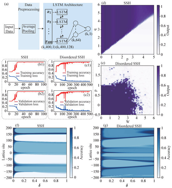
Figure 5.
Training of LSTM. (a) Structure diagram of LSTM. k is the number of samples. (b1,b2) The accuracy (red line) and loss (blue line) of the (b1) training set and (b2) validation set as functions of epoch when training the LSTM identify the topology of the SSH model. (c1,c2) The accuracy (red line) and loss (blue line) of the (c1) training set and (c2) validation set as functions of epoch when training the LSTM identify the topology of the disordered SSH model. (d) The output of the trained LSTM varies with the parameters p and q of the SSH model. (e) The output of the trained LSTM varies with the parameters p and W of the disordered SSH model. (f,g) Prediction accuracy of (f) SSH and (g) disordered SSH model for input data with different deviations at different lattice sites. The parameter settings for generating input data are set as , , , and .
Figure 5d and Figure 5e respectively show the changes in the LSTM network output with the parameters p and q of the SSH model, and with the parameters p and W of the disordered SSH model. It can be seen that the LSTM network can still roughly identify the topology of the SSH model and the disordered SSH model. However, more discrete error points appear at the topological boundary of the disordered SSH model.
Figure 5f,g show the accuracy of the LSTM network in identifying the topology of the SSH model and the disordered SSH model for different errors at different lattice sites. The sensitivity of the LSTM network to the errors of the SSH model and the disordered SSH model exhibits regional characteristics. It is quite sensitive to errors within a range of lattice sites, while relatively insensitive to errors in another range.
By comparing the training results of three types of networks, we found that there is no significant difference among the three networks in terms of the topological recognition ability for the SSH model. However, the vanilla RNN and LSTM networks require more epochs to achieve better training results. Regarding the topological recognition ability for the disordered SSH model, it weakens as the network complexity increases, and the training time cost also significantly rises with the increase in complexity. In contrast, the FNN is more suitable for identifying the topology of the SSH model and the disordered SSH through population dynamics.
5. Prediction Accuracy for Different Input Data
In this section, we discuss the recognition accuracies of three trained networks for the SSH model and the disordered SSH model on input data under different conditions of the number of unit cells N, time length T, number of time points , and generation counts .
The discussion about the situation of the SSH model is shown in Figure 6. First, we discuss how the prediction accuracy changes with the number of unit cells N. Since our network is trained based on a model with 200 unit cells, when identifying models with less than 200 unit cells, we add zeros on both sides of the input data to expand it to 200 unit cells. When identifying models with than more 200 unit cells, we extract the input data of the middle 200 unit cells. The prediction accuracies of the three networks are shown in Figure 6a. When the number of unit cells is large, the prediction accuracies of the three networks can all approach . This is because within the time length we set, the population dynamics have not reached the model boundary. The error caused by back propagation after the dynamics reach the boundary is not significant, so the prediction accuracy does not change significantly. When the number of unit cells N is small, the error generated by back propagation after the dynamics reach the boundary begins to increase. This error is mainly concentrated around the lattice sites ± N. Through the sensitivity analysis of the input data of the SSH model by the three networks shown in Figure 3f, Figure 4f and Figure 5f, we can see that when the number of unit cells is around 100, the vanilla RNN and LSTM networks start to become sensitive to the error, and the accuracy begins to decline rapidly and the FNN still maintains a relatively high accuracy, as shown in Figure 6a.
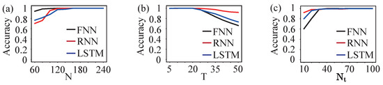
Figure 6.
Prediction accuracy of three networks for the topology of the SSH model under different input data. (a) Prediction accuracy under different numbers of cells N, with the number of time points and the time length . (b) Prediction accuracy under different time lengths T, with the number of time points and the number of cells . (c) Prediction accuracy under different numbers of time points , with the number of cells and the time length .
Then we discussed the case where the number of unit cells in the SSH model is and the time length T increases. At this time, the error still stems from the fact that the dynamics reach the boundary and then propagate backward. Therefore, when T is small, the prediction accuracies of all three networks are high. As T increases, the errors near the lattice points ± 200 will increase. According to the previous sensitivity analysis, it can be seen that the prediction accuracy of the vanilla RNN should be the highest, followed by the LSTM network, and finally the FNN, as shown in Figure 6b.
For the case of changing the number of time points , when the number of time points increases, no errors will occur. Therefore, the prediction accuracies of the three networks are all very high. When the number of time points decreases, errors will appear at each lattice site. At this time, we compare the size of the lattice site ranges to which these three networks are sensitive and their sensitivities to the magnitude of the error values. As shown in Figure 6c, the vanilla RNN has the best anti-interference ability against changes in the number of time points, followed by the LSTM network, and finally FNN.
The discussion on the case of the disordered SSH model is shown in Figure 7. Since disorder induces localization, as shown in Figure 2(c1,d1), the population dynamics do not spread to both sides. Therefore, within the range of the selected unit cell number N, time length T, and number of time points , the prediction accuracies of the three networks did not show any significant changes. As for the generation counts , when it increases, there will be no errors and the prediction accuracy remains consistently high. When it decreases, errors occur at the local lattice sites of the population. At this time, FNN has the strongest anti-interference ability, followed by vanilla RNN, and finally LSTM networks.
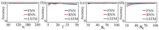
Figure 7.
Prediction accuracy of three networks for the topology of the disordered SSH model under different input data. (a) Prediction accuracy under different numbers of cells N, with the number of time points , the time length and generation counts . (b) Prediction accuracy under different time lengths T, with the number of time points , the number of cells and generation counts . (c) Prediction accuracy under different numbers of time points , with the number of cells , the time length and generation counts . (d) Prediction accuracy under different generation counts , with the number of cells , the time length and numbers of time points .
6. Front-End Application
In this section, we introduced a winding number prediction tool for the disordered SSH model, which is developed based on the Vue.js front-end and Flask back-end frameworks and uses the LSTM network for prediction.
Front-end Design. The front-end is implemented using Vue.js, a powerful, high-performance, and easy-to-learn JavaScript framework. Its core features, a progressive architecture, a lightweight component-based design, and an efficient reactive data-binding mechanism, make it one of the most widely adopted front-end frameworks. Vue provides responsive rendering, modular code organization, and seamless state management, making it well suited for dynamic, real-time applications. In our interface, as shown in Figure 8, users can input two parameters: W and p. These values are entered through numeric input fields equipped with built-in range validation to prevent invalid or out-of-bound entries. Once the inputs are submitted, the system dynamically visualizes both the input settings and the network prediction result, enabling an intuitive understanding of how the network behaves under different conditions.
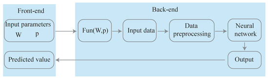
Figure 8.
Schematic diagram of the prediction tool, consisting of a front-end for input parameters and a back-end for processing and output.
Back-end Design. The back-end is implemented in Python 3.9.6 using the Flask framework, which provides a simple and flexible Representational State Transfer Application Programming Interface (REST API) architecture. Flask is a lightweight web application framework known for its clarity, extensibility, and ease of development. Its built-in development server significantly streamlines debugging, experimentation, and iterative testing. When the front-end submits user-defined parameters , Flask receives the HyperText Transfer Protocol (HTTP) request. Then, as shown in Figure 8, use the Fun(W, p) function to generate the population dynamics when the number of unit cells , the time length , the number of time points , and generation counts as the input data. Perform preprocessing on the input data, including average pooling, data balancing, and standardization. Input the processed data into the trained LSTM network to obtain the network output. After computation, the prediction is serialized into JSON format and transmitted back to the front-end visualization modules.
7. Conclusions
We discussed the ability of FNN, vanilla RNN, and LSTM networks to identify the topology of the SSH model and the disordered SSH model by taking the population dynamics as the input of the neural networks. We found that with appropriate input data, all three networks can accurately identify the topology of the two models. If the input data changes, the abilities of the three networks to identify topology will also vary. For the identification of the topology of the SSH model, if the number of unit cells N in the input data decreases, the FNN has the highest prediction accuracy; if the time length T increases and the number of time points decreases, the vanilla RNN has the highest prediction accuracy. For the disordered SSH model, when changing the number of unit cells N, the time length T, and the number of time points , there is no significant difference in the prediction accuracies of the three networks. When reducing the number of generations , the FNN has the highest prediction accuracy.
Furthermore, we have developed and deployed a topological invariant prediction tool based on a Vue.js front-end and a Flask back-end framework. This tool allows users to input parameters in real time and obtain predictions of topological invariants, enabling direct integration between theoretical models and end-user applications. This study not only validates the effectiveness of LSTM networks in predicting disordered topological systems but also provides a ready-to-use tool to facilitate exploration and prediction in related fields, thereby establishing a crucial foundation for data-driven research in complex topological systems.
Author Contributions
Conceptualization, Y.S. and Y.H.; methodology, Y.Y.; software, Y.Y. and Z.F.; validation, Y.Y.; formal analysis, Y.Y. and Y.S.; investigation, Y.Y.; data curation, Y.Y.; writing—original draft preparation, Y.Y.; writing—review and editing, Y.Y. and Y.S.; visualization, Y.Y. and Y.S. All authors have read and agreed to the published version of the manuscript.
Funding
This research is funded by the National Natural Science Foundation of China (Grants No. 12374246). Y.H. acknowledges support from the Beijing National Laboratory for Condensed Matter Physics (No. 2023BNLCMPKF001).
Data Availability Statement
The original contributions presented in this study are included in the article. Further inquiries can be directed to the corresponding author.
Conflicts of Interest
The authors declare no conflicts of interest.
Abbreviations
The following abbreviations are used in this manuscript:
| FNN | Feedforward neural network |
| RNN | Recurrent neural network |
| LSTM | Long short-term memory network |
| SSH | Su–Schrieffer–Heeger |
| h.c. | Hermitian conjugate |
| REST API | Representational state transfer application programming interface |
| HTTP | Hypertext transfer protocol |
References
- Zak, J. Berry’s Phase for Energy Bands in Solids. Phys. Rev. Lett. 1989, 62, 2747. [Google Scholar] [CrossRef]
- Hatsugai, Y. Chern Number and Edge States in the Integer Quantum Hall Effect. Phys. Rev. Lett. 1993, 71, 3697. [Google Scholar] [CrossRef]
- Fu, L.; Kane, C.L.; Mele, E.J. Topological Insulators in Three Dimensions. Phys. Rev. Lett. 2007, 98, 106803. [Google Scholar] [CrossRef] [PubMed]
- Xiao, D.; Chang, M.C.; Niu, Q. Berry Phase Effects on Electronic Properties. Rev. Mod. Phys. 2010, 82, 1959. [Google Scholar] [CrossRef]
- Hasan, M.Z.; Kane, C.L. Colloquium: Topological Insulators. Rev. Mod. Phys. 2010, 82, 3045. [Google Scholar] [CrossRef]
- Qi, X.L.; Zhang, S.C. Topological Insulators and Superconductors. Rev. Mod. Phys. 2011, 83, 1057. [Google Scholar] [CrossRef]
- Khanikeav, A.B.; Mousavi, S.H.; Tse, W.K.; Kargarian, M.; MacDonald, A.H.; Shveys, G. Photonic Topological Insulator. Nat. Mater. 2013, 12, 233–239. [Google Scholar] [CrossRef]
- Rechtsman, M.C.; Zeuner, J.M.; Plotnik, Y.; Lumer, Y.; Podolsky, D.; Dreisow, F.; Nolte, S.; Segev, M.; Szameit, A. Photonic Floquet Topological Insulators. Nature 2013, 496, 196–200. [Google Scholar] [CrossRef]
- Chiu, C.K.; Teo, J.C.Y.; Schnyder, A.P.; Ryu, S. Classification of Topological Quantum Matter with Symmetries. Rev. Mod. Phys. 2016, 88, 035005. [Google Scholar] [CrossRef]
- Bansil, A.; Lin, H.; Das, T. Colloquium: Topological Band Theory. Rev. Mod. Phys. 2016, 88, 021004. [Google Scholar] [CrossRef]
- Wen, X.G. Colloquium: Zoo of Quantum-Topological Phases of Matter. Rev. Mod. Phys. 2017, 89, 041004. [Google Scholar] [CrossRef]
- Pöyhönen, K.; Sahlberh, I.; Westström, A.; Ojanen, T. Amorphous Topological Superconductivity in a Shiba Glass. Nat. Commun. 2018, 9, 2103. [Google Scholar] [CrossRef] [PubMed]
- Titum, P.; Lindner, N.H.; Rechtsman, M.C.; Refael, G. Disorder-Induced Floquet Topological Insulators. Phys. Rev. Lett. 2015, 114, 056801. [Google Scholar] [CrossRef]
- Liu, C.; Gao, W.; Yang, B.; Zhang, S. Disorder-Induced Topological State Transition in Photonic Metamaterials. Phys. Rev. Lett. 2017, 119, 183901. [Google Scholar] [CrossRef]
- Agarwala, A.; Shenoy, V.B. Topological Insulators in Amorphous Systems. Phys. Rev. Lett. 2017, 118, 236402. [Google Scholar] [CrossRef]
- Meier, E.J.; An, F.A.; Dauphin, A.; Maffei, M.; Massignan, P.; Hughes, T.L.; Gadway, B. Observation of the Topological Anderson Insulator in Disordered Atomic Wires. Science 2018, 362, 929–933. [Google Scholar] [CrossRef]
- Sahlberh, I.; Westström, A.; Pöyhönen, K.; Ojanen, T. Topological Phase Transitions in Glassy Quantum Matter. Phys. Rev. Res. 2020, 2, 013053. [Google Scholar] [CrossRef]
- Wang, A.A.; Zhao, Z.; Ma, Y.; Cai, Y.; Zhang, R.; Shang, X.; Zhang, Y.; Qin, J.; Pong, Z.K.; Marozsák, T.; et al. Topological Protection of Optical Skyrmions Through Complex Media. Light-Sci. Appl. 2024, 13, 314. [Google Scholar] [CrossRef] [PubMed]
- Guo, Z.; Peters, C.; Cervera, N.M.; Vetlugin, A.; Guo, R.; Zhang, P.; Forbes, A.; Shen, Y. Topological Robustness of Classical and Quantum Optical Skyrmions in Atmospheric Turbulence. arXiv 2025, arXiv:2509.05727. [Google Scholar] [CrossRef]
- Carrasquilla, J.; Melko, R.G. Machine Learning Phases of Matter. Nat. Phys. 2017, 13, 431–434. [Google Scholar] [CrossRef]
- Broecker, P.; Carrasquilla, J.; Melko, R.G.; Trebst, S. Machine Learning Quantum Phases of Matter beyond the Fermion Sign Problem. Sci. Rep. 2017, 7, 8823. [Google Scholar] [CrossRef]
- van Nieuwenburg, E.P.L.; Liu, Y.H.; Huber, S.D. Learning Phase Transitions by Confusion. Nat. Phys. 2017, 13, 435–439. [Google Scholar] [CrossRef]
- Beach, M.J.S.; Golubeva, A.; Melko, R.G. Machine Learning Vortices at the Kosterlitz-Thouless Transition. Phys. Rev. B 2018, 97, 045207. [Google Scholar] [CrossRef]
- Sun, N.; Yi, J.; Zhang, P.; Shen, H.; Zhai, H. Deep Learning Topological Invariants of Band Insulators. Phys. Rev. B 2018, 98, 085402. [Google Scholar] [CrossRef]
- Zhang, P.; Shen, H.; Zhai, H. Machine Learning Topological Invariants with Neural Networks. Phys. Rev. Lett. 2018, 120, 066401. [Google Scholar] [CrossRef] [PubMed]
- Rem, B.S.; Käming, N.; Tarnowaki, M.; Asteria, L.; Fläschner, N.; Becker, C.; Sengstock, K.; Weitenberg, C. Identifying Quantum Phase Transitions Using Artificial Neural Networks on Experimental Data. Nat. Phys. 2019, 15, 917–920. [Google Scholar] [CrossRef]
- Che, Y.; Gneiting, C.; Liu, T.; Nori, F. Topological Quantum Phase Transitions Retrieved through Unsupervised Machine Learning. Phys. Rev. B 2020, 102, 134213. [Google Scholar] [CrossRef]
- Balabanov, O.; Granath, M. Unsupervised Learning Using Topological Data Augmentation. Phys. Rev. Res. 2020, 2, 013354. [Google Scholar] [CrossRef]
- Yu, L.W.; Deng, D.L. Unsupervised Learning of Non-Hermitian Topological Phases. Phys. Rev. Lett. 2021, 126, 240402. [Google Scholar] [CrossRef]
- Molognini, P.; Zegarra, A.; van Nieuwenburg, E.; Chitra, R.; Chen, W. A Supervised Learning Algorithm for Interacting Topological Insulators based on Local Curvature. SciPost Phys. 2021, 11, 073. [Google Scholar] [CrossRef]
- Zhang, L.F.; Tang, L.Z.; Huang, Z.H.; Zhang, G.Q.; Huang, W.; Zhang, D.W. Machine Learning Topological Invariants of Non-Hermitian Systems. Phys. Rev. A 2021, 103, 012419. [Google Scholar] [CrossRef]
- Kuo, E.J.; Dehghani, H. Unsupervised Learning of Interacting Topological and Symmetry-Breaking Phase Transitions. Phys. Rev. B 2022, 105, 235136. [Google Scholar] [CrossRef]
- Zhao, E.; Mak, T.H.; He, C.; Ren, Z.; Pak, K.K.; Liu, Y.J.; Jo, G.B. Observing a Topological Phase Transition with Deep Neural Networks from Experimental Images of Ultracold Atoms. Opt. Express 2022, 30, 37786–37794. [Google Scholar] [CrossRef]
- Chen, J.; Wang, Z.; Tan, Y.T.; Wang, C.; Ren, J. Machine Learning of Knot Topology in Non-Hermitian Band Braids. Commun. Phys. 2024, 7, 209. [Google Scholar] [CrossRef]
- Pan, G.Z.; Yang, M.; Zhou, J.; Yuan, H.; Miao, C.; Zhang, G. Quantifying Entanglement for Unknown Quantum States via Artificial Neural Networks. Sci. Rep. 2024, 14, 26267. [Google Scholar] [CrossRef]
- Zhang, Z.; Kong, L.; Zhang, L.; Pan, X.; Das, T.; Wang, B.; Liu, B.; Wang, F.; Nape, I.; Shen, Y.; et al. Structured Light Meets Machine Intelligence. eLight 2025, 5, 26. [Google Scholar] [CrossRef]
- Holanda, N.L.; Griffith, M.A.R. Machine Learning Topological phases in Real Space. Phys. Rev. B 2020, 102, 054107. [Google Scholar] [CrossRef]
- Lusing, E.; Yair, O.; Talmon, R.; Segev, M. Identifying Topological Phase Transitions in Experiments Using Manifold Learning. Phys. Rev. Lett. 2020, 125, 127401. [Google Scholar] [CrossRef]
- Yu, Y.; Yu, L.W.; Zhang, W.; Zhang, H.; Ouyang, X.; Liu, Y.; Deng, L.D.; Duan, L.M. Experimental Unsupervised Learning of Non-Hermitian Knotted Phased with Solid-state Spins. npj Quantum Inf. 2022, 8, 116. [Google Scholar] [CrossRef]
- Hochreiter, S.; Schmidhuber, J. Long Short-Term Memory. Neural Comput. 1997, 9, 1735–1780. [Google Scholar] [CrossRef]
- Graves, A.; Schmidhuber, J. Framewise Phoneme Classification with Bidirectional LSTM and Other Neural Network Architectures. Neural Netw. 2005, 18, 602–610. [Google Scholar] [CrossRef]
- August, M.; Ni, X. Using Recurrent Neural Network to Optimize Dynamical Decoupling for Quantum Memory. Phys. Rev. A 2005, 95, 012335. [Google Scholar]
- Walters, M.; Wei, Q.; Chen, J.Z.Y. Machine Learning Topological Defects of Confined Liquid Crystals in Two Dimensions. Phys. Rev. E 2019, 99, 062701. [Google Scholar] [CrossRef]
- Vandans, O.; Yang, K.; Wu, Z.; Dai, L. Identifying Knot Types of Polymer Conformations by Machine Learning. Phys. Rev. E 2020, 101, 022502. [Google Scholar] [CrossRef]
- Goh, H.A.; Ho, C.K.; Absas, F.S. Front-end Deep Learning Web Apps Development and Deployment: A Review. Appl. Intell. 2023, 53, 15923–15945. [Google Scholar] [CrossRef]
- Anderson, P.W. Absence of Diffusion in Certain Random Lattices. Phys. Rev. 1958, 109, 1492. [Google Scholar] [CrossRef]


Disclaimer/Publisher’s Note: The statements, opinions and data contained in all publications are solely those of the individual author(s) and contributor(s) and not of MDPI and/or the editor(s). MDPI and/or the editor(s) disclaim responsibility for any injury to people or property resulting from any ideas, methods, instructions or products referred to in the content. |
© 2026 by the authors. Licensee MDPI, Basel, Switzerland. This article is an open access article distributed under the terms and conditions of the Creative Commons Attribution (CC BY) license.