Article

Artificial Neural Network Modeling of Darcy–Forchheimer Nanofluid Flow over a Porous Riga Plate: Insights into Brownian Motion, Thermal Radiation, and Activation Energy Effects on Heat Transfer

by
Zafar Abbas
1,
Aljethi Reem Abdullah
2,
Muhammad Fawad Malik
3,* and
Syed Asif Ali Shah
4
1
Centre for High Energy Physics, University of the Punjab, Lahore 54590, Pakistan
2
Department of Mathematics and Statistics, College of Science, Imam Mohammad Ibn Saud Islamic University (IMSIU), Riyadh 11432, Saudi Arabia
3
Department of Mathematics, Government College University, Faisalabad 38000, Pakistan
4
Department of Modern Mechanics, School of Engineering Science, University of Science and Technology of China, Hefei 230026, China
*
Author to whom correspondence should be addressed.
Symmetry 2025, 17(9), 1582; https://doi.org/10.3390/sym17091582
Submission received: 12 August 2025 / Revised: 8 September 2025 / Accepted: 11 September 2025 / Published: 22 September 2025
(This article belongs to the Special Issue Computational Mathematics and Its Applications in Numerical Analysis)

Abstract

Nanotechnology has become a transformative field in modern science and engineering, offering innovative approaches to enhance conventional thermal and fluid systems. Heat and mass transfer phenomena, particularly fluid motion across various geometries, play a crucial role in industrial and engineering processes. The inclusion of nanoparticles in base fluids significantly improves thermal conductivity and enables advanced phase-change technologies. The current work examines Powell–Eyring nanofluid’s heat transmission properties on a stretched Riga plate, considering the effects of magnetic fields, porosity, Darcy–Forchheimer flow, thermal radiation, and activation energy. Using the proper similarity transformations, the pertinent governing boundary-layer equations are converted into a set of ordinary differential equations (ODEs), which are then solved using the boundary value problem fourth-order collocation (BVP4C) technique in the MATLAB program. Tables and graphs are used to display the outcomes. Due to their significance in the industrial domain, the Nusselt number and skin friction are also evaluated. The velocity of the nanofluid is shown to decline with a boost in the Hartmann number, porosity, and Darcy–Forchheimer parameter values. Moreover, its energy curves are increased by boosting the values of thermal radiation and the Biot number. A stronger Hartmann number M decelerates the flow (thickening the momentum boundary layer), whereas increasing the Riga forcing parameter Q can locally enhance the near-wall velocity due to wall-parallel Lorentz forcing. Visual comparisons and numerical simulations are used to validate the results, confirming the durability and reliability of the suggested approach. By using a systematic design technique that includes training, testing, and validation, the fluid dynamics problem is solved. The model’s performance and generalization across many circumstances are assessed. In this work, an artificial neural network (ANN) architecture comprising two hidden layers is employed. The model is trained with the Levenberg–Marquardt scheme on reliable numerical datasets, enabling enhanced prediction capability and computational efficiency. The ANN demonstrates exceptional accuracy, with regression coefficients R 1.0 and the best validation mean squared errors of 8.52 × 10 10 , 7.91 × 10 9 , and 1.59 × 10 8 for the Powell–Eyring, heat radiation, and thermophoresis models, respectively. The ANN-predicted velocity, temperature, and concentration profiles show good agreement with numerical findings, with only minor differences in insignificant areas, establishing the ANN as a credible surrogate for quick parametric assessment and refinement in magnetohydrodynamic (MHD) nanofluid heat transfer systems.

1. Introduction

Nanofluids are engineered fluids created by dispersing nanometer-scale particles, such as metals, metal oxides, carbides, and carbon nanotubes, into conventional base fluids. These suspensions exhibit enhanced thermophysical properties, making them highly effective for improving heat transfer efficiency. Applications of nanofluids extend across diverse fields, including high-performance heat exchangers, advanced cooling systems, thermal management in electronics, biomedical processes, hybrid power systems, and domestic refrigeration. At present, there exist three principal coupling models. The initial model is the data-driven paradigm, which facilitates the derivation of the input–output relationship devoid of any physical mechanisms. The subsequent model is the physical framework, which seeks to enhance the preexisting models through the application of artificial intelligence algorithms. The single-phase Buongiorno model (2006), which takes thermophoresis slip and Brownian diffusion into consideration, is used in this paper. It is generally acknowledged that this model is a useful foundation for forecasting the movement of nanoparticles in convective boundary layers. The tertiary model is a hybrid approach that integrates both data-driven and physical mechanisms. Among the diverse array of artificial intelligence algorithms, the ANN is predominantly utilized to construct data-driven models and has been effectively implemented across five domains, specifically aerodynamic modeling, turbulence modeling, certain specialized flows, and mass and heat transfer phenomena. Other artificial intelligence algorithms, including recursive neural networks (RNNs), support vector machines (SVMs), and naive Bayes (NB) algorithms, are primarily employed in the context of physical models.
Non-Newtonian fluids exhibit varying viscosities in response to applied forces, in contrast to conventional fluids like water or oil, which have a constant viscosity independent of agitation or compression. The viscosity of these fluids lowers with the rise in shear rate. Before a specific stress barrier is crossed, non-Newtonian fluids act like solids; they flow as Newtonian fluids. Some drilling fluids and toothpaste exhibit similar characteristics. We refer to this kind of conduct as Bingham plastic behavior. Non-Newtonian fluids include a variety of molten polymers, salt solutions, custard, paint, fabric composites, toothpaste, starch suspensions, and blood. Evaluating the possible benefits of fluids with lower drag has been the main area of research for non-Newtonian flows. For example, research on drag measurements of low-concentration polymer solutions in pipe flows was published by Berman [1]. Non-Newtonian fluid flows occur not just in the natural world but also in many fields depending on heat processes. The refinement of the Laval high-frequency atomizing nozzle’s structural characteristics and gas–liquid two-phase flow law were examined by Guo et al. [2]. Their research focused on the spontaneous convection process that takes place in a homogeneous, incompressible fluid that is trapped between two infinite, concentric vertical cylinders. Unexpectedly, certain materials with non-Newtonian fluid qualities may balance shielding from high-speed strikes with flexibility, making them useful for body armor, padding systems, and shock absorbers.
Investigators developed nanofluids, a novel type of fluids which are composed of single nanoparticles submerged in the base fluid; these are more effective at transporting heat than normal fluids. They are revolutionary and prospective operating fluids because of their excellent heat transfer coefficient, thermal conductivity, and viscosity features. The uses of nanofluids are multidisciplinary and involve electronic cooling systems in automotive systems, energy production from renewable sources, and cancer treatment. In terms of efficiency and organization, nanofluids expedite and refine the process. These have several uses across various industries, including biotechnology, processors, nanotechnology, radiation therapy, and refrigeration. The initial study on the augmentation of a fluid’s thermal conductivity due to the dispersion of extremely fine particles was made by Masuda et al. [3]. Nanofluids are very important in the world of thermal transmission technology. Nanofluids are fluids that contain nano-sized particles to improve thermal characteristics and change the dynamics of fluids, as described by Choi [4]. Later, when copper nanoparticles were incorporated into ethylene glycol at a volume concentration of 0.3, Eastman et al. [5] saw a 40% increase in thermal conductivity. Awais et al. [6] investigated the influence of nanofluids on the thermo-hydraulic behavior of heating systems, providing guidance for their effective selection and application in industrial heating devices. Yaseen et al. [7] addressed the mass and heat transport for a micropolar nanofluid with MHD effects when there is transpiration from an annular body. Wu et al. [8] investigated the very effective capillary-fed boiling heat transfer using grooved-porous synthetic wick architectures.
Buongiorno [9] addressed convectional thermal transfer and activity in nanofluids. Owhaib and Al-Kouz [10] theoretically investigated the thermal transmission properties of copper/water nanofluid flow across a dual-direction stretchable membrane using the Buongiorno model. Using the previously described model, Wang et al. [11] investigated the heat transmission that occurs when a thin film passes through a stretched sheet that is susceptible to temperature and velocity slips. Sindhu et al. [12] used a modified Buongiorno model to study the convective heat transfer of nanoliquid during slip and convection phase in tiny channels. Zhu et al. [13] examined how thermoelectric generator systems with and without stepped configurations performed in terms of contrast and refinement. A newly formulated relaxation time expression was incorporated into the lattice Boltzmann framework, enabling more accurate and efficient simulation of transient flow through porous nanostructures, by Zarei et al. [14].
The study of electrically conductive fluids in the presence of magnetic fields is known as MHD. It is a branch of physical science that studies the behavior of liquids that transmit electricity and magnetism, including plasma, seawater, electrolytes, and liquid metals. Magnetism is a subject of tremendous relevance in applications worldwide, playing a role in many technical and industrial advances due to its capacity to modify the flow field. Ibrahim et al.’s analysis [15] looked at how nonlinear electrical radiation and viscous scattering affected steady flow in the context of MHD. Hayat et al. [16] investigated the behavior of MHD flow and associated heat transfer when a porous stretching sheet was considered with velocity slip at the boundary. Patel et al. [17] examined the MHD flow of a micropolar nanoliquid using magnetite as a basic fluid. Convective heat transfer is heat being transferred from one location to another via the flow of fluids. This is the combination of conduction and advection, which are terms used interchangeably, for bulk fluid movement and heat diffusion. Convective heat transfer has widespread use in the fields of engineering and technology. These small particles are made up of metals, oxides, carbides, etc. Because of their capabilities, nanofluids may be useful in a variety of heat exchange applications. Their thermal conductivity and convective heat are enhanced. Fluid mechanics is a scientific discipline concerned with understanding the physical characteristics of fluids and analyzing their behavior under conditions of rest (fluid statics) or motion (fluid dynamics). It may be used in a wide range of scientific fields. Numerous businesses employ a variety of fluid types, including ions, liquids, micropolar fluids, and oil reservoirs. By examining the flow of atmospheric fluids on Earth, weather experts may forecast conditions using the principles of fluid mechanics. Nonlinear heat radiation effects on Williamson nanofluid flowing past a stretching surface were observed by Ganesh Kumar et al. [18]. A numerical simulation of a stretched cylinder with heat radiation and convective boundary conditions, utilizing Williamson nanofluid, was conducted by Bilal et al. [19]. The characteristics of Maxwell tiny fluids in the context of MHD flow and hot irradiation were studied by Rashid et al. [20]. The release of electromagnetic waves from an object’s surface as a result of high temperatures is known as thermal radiation. Thermal radiation, which may consist of infrared, visible, ultraviolet, and even electromagnetic radiation, is emitted by all things that are above absolute zero. Li et al. [21] suggested crucial heat flow and nucleate boiling heat transfer in controlled droplet train chilling. The temperature of an object and the composition of its outermost material determine how much and what kind of thermal radiation it emits. An object’s temperature causes it to produce more thermal radiation, which has fewer wavelengths as it grows hotter. This natural occurrence explains why, based on their temperature, hot objects generate a red, yellow, or white glow. The fluid dynamics and thermal radiation consequences of a magnetized hybrid nanofluid were studied by Tayebi et al. [22]. Hayat et al. [23] investigated the use of chemical characteristics and thermal influence on the MHD flow through the boundary layer of nanofluid.
Activation energy is the smallest amount of energy required for a specific reaction to occur in a given species. It is the lowest energy level that reactants must possess to initiate a chemical reaction. The nonlinear degradation contributions are scaled using the Arrhenius activation-energy term in γ 1 and γ 2 . Higher E decreases response rates and lessens the impact of viscous dissipation coupling because it creates heating/cooling rates dependent upon activation energy. Maleque [24] investigated the impact of energy activation on both endothermic and exothermic chemical processes and analyzed the associated effects. Arshad et al. [25] provided a comprehensive review of the flow of a chemically reactive nanofluid past a slender moving needle. The simultaneous impacts of the above mentioned energy and chemical reactions on the flow of MHD fluid across a horizontally expanding surface were examined by Lakshmi et al. [26].
Artificial neural networks are computer models made up of neurons that are linked together and are inspired by the composition and operations of the human brain. Explicit programming is not necessary to develop predictions based on data patterns. Fluid mechanics applications include predicting flow, modeling turbulence, estimating properties, improving systems, and regulating flows. ANNs support these tasks by optimizing system performance, generating turbulence models, and accurately forecasting flow behavior. Ahmedi et al. [27] estimated pressure decreases in automobile radiators with nanofluids using ANN systems combined with genetic algorithms. Hojjat. [28] employed multi-objective optimization and ANN modeling for nanofluids utilized as coolants in shell and tube heat exchanger setups. An excellent technique for modeling Darcy–Forchheimer Ree–Eyring fluid flow against a porous stretching layer with activation energy and a convective boundary condition is an ANN, according to research by Shafiq et al. [29]. According to [30], the built ANN is a powerful engineering technique that can provide forecasts with a very high degree of accuracy and be applied to dependability analysis via the inverse power law with Bayesian regularization. Kamsuwan et al. [31] employed ANNs to imitate a microchannel heat exchanger with nanoliquid streams and improved the simulation by incorporating nanofluid characteristics. Jery et al. [32] developed an ANN framework for nanoliquid heat exchangers, enabling accurate prediction of heat transfer rates, Nusselt number variations, and entropy generation.

2. Problem Statement

This work examines the continuous, incompressible, two-dimensional flow of a Powell–Eyring nanofluid via a porous Riga plate. A wall-parallel Lorentz force that affects the near-wall fluid motion is produced by the alternating electrodes and magnets that make up the Riga surface. Darcy–Forchheimer drag and the porous medium, which contribute more resistive forces, further alter the flow as shown in Figure 1. The y-axis is parallel to the flow direction in Figure 1, whereas the x-axis is aligned with it. In the Riga plate configuration, the surface is embedded with alternating strips of magnets and electrodes. The geometric dimension of these elements is expressed by the parameter s, which influences the generated electromagnetic forcing. A magnetic field B 1 ( x ) = B 0 ( x + b ) m 1 2 , which is not consistent when applied across a plate. The electromagnetic field M of the Riga plate produces a wall-parallel Lorentz force that decays exponentially. Furthermore, if the power index of velocity is m, it is assumed that the sheet is not planar. To ensure that the sheet stays suitably thin, we are going to assume that d is very tiny. At this point, the temperature and concentration of the nanoparticles on the surface are constant at T ˜ w and C ˜ w , whereas the temperature and concentration of the surroundings are distant from the surface area T ˜ , C ˜ , respectively. When the electromagnetic field of the Riga plate interacts with the base fluid’s nanoparticles, the Lorentz force is produced. The governing equations, such as continuity, velocity, temperature and concentrations, are given as
u ˜ x + v ˜ y = 0 ,
u ˜ u ˜ x + v ˜ u ˜ y = ν n f + 1 ρ n f β 1 u ˜ y y + π j * M 8 ρ n f e π y a 1 σ ˜ ρ n f B 1 2 ( x ) u ˜ 1 2 ρ n f β 1 3 ( u ˜ y ) 2 u ˜ y y ν k u ˜ F 0 u ˜ 2 ,
u ˜ T ˜ x + v ˜ T ˜ y = K n f ( ρ c p ) n f T ˜ y y 1 + 16 σ * T ˜ 3 3 k k * + τ ˜ D ˜ B C ˜ y T ˜ y + D ˜ T T ˜ ( T ˜ y ) 2 + σ ˜ ( ρ c p ) n f B 1 2 ( x ) u ˜ 2 ,
u ˜ C x ˜ + v ˜ C y ˜ = D B ˜ C y y ˜ + D T ˜ T T ˜ y y k r 2 ( C ˜ C ˜ ) exp E a K T ˜ T ˜ T ˜ n ,
along with
u ˜ = U w , T y ˜ ( k ) = ( T ˜ + T ˜ f ) h 1 , v ˜ = 0 , C ˜ y 1 ˜ ( D ˜ B ) = h 2 ( C ˜ W C ˜ ) , as y = 0 , u ˜ 0 , C ˜ C ˜ , T ˜ T ˜ , a s y ,
In contrast, similarity transformations are
ψ = 2 m + 1 v ˜ U 0 ( x + b ) m + 1 1 2 f ( η ) , η = ( m + 1 2 ) U 0 ( x + b ) m 1 v ˜ 1 2 θ ( η ) = T ˜ T ˜ T ˜ f T ˜ , u ˜ = U 0 ( x + b ) m f ( η ) v ˜ = m + 1 2 v ˜ U 0 ( b + x ) 1 + m 1 2 f ( η ) + η m 1 m + 1 f ( η ) , ϕ ( η ) = C ˜ C ˜ C ˜ w C ˜
and ODEs are
f f f 2 ( 2 m m + 1 ) f 2 f ( m + 1 2 ) N λ + Q exp ( β η ) ( 2 m + 1 ) M f + ( 1 + N ) f δ f F r f 2 = 0 ,
P r θ ϕ N b + N t θ 2 + f θ + 1 + 4 3 R d θ + P r 2 m + 1 M E c ( f ) 2 + P r γ 1 m 3 2 f f θ m + 1 2 θ f 2 = 0 ,
ϕ + N t N b θ + P r L e γ 2 ϕ m 3 2 f f ϕ m + 1 2 f 2 + P r L e ( f ϕ ) P r L e σ ( 1 + δ ˜ θ ) n exp E ( 1 + δ ˜ θ ) ϕ = 0 .
The Powell–Eyring constitutive model’s nonlinear viscous dissipation and variable-property contributions are represented by the extra terms corresponding to γ 1 and γ 2 , which emerge following the similarity transformation of higher-order stress factors.
Corresponding boundary conditions are
f ( 0 ) = 1 , f ( 0 ) = 0 , ϕ ( 0 ) = α 1 ( 1 ϕ ( 0 ) ) , θ ( 0 ) = B i ( 1 θ ( 0 ) ) as η = 0 , f ( ) 0 , θ ( ) 0 , ϕ ( ) 0 as η .
Here, B i is the thermal Biot number and α 1 is the concentration slip coefficient.
Parameter values are
P r = v α , Q = π J 0 M 0 ( x + b ) 8 ρ n f U 0 2 , β = π a ( m + 1 ) U 0 ( x + b ) m 1 2 v ˜ 1 2 , B i = h s k 2 U 0 ( x + b ) m 1 ( m + 1 ) v ˜ 1 2 L e = α D ˜ B , α = k ρ c p , N b = τ D ˜ B v ˜ C ˜ , N t = τ D ˜ T v ˜ T ˜ T ˜ f T ˜ , τ n p = ( ρ C p ) p ( ρ C p ) f , γ 1 = λ E U 0 ( x + b ) m 1 , λ = U 0 ( x + b ) 3 m 1 2 v ˜ C ˜ 2 , E c = U 0 2 ( x + b ) 2 m c p ( T ˜ f T ˜ ) , M = σ ˜ B 0 2 ρ U 0 , K 1 = k 0 ( m + 1 ) U 0 2 v ˜ 1 2 , N = 1 μ β c , γ 2 = λ E U 0 ( x + b ) m 1 , F r = C b K 1 2 , δ = ν K a , R d = 4 σ * T ˜ 3 k k * , δ ˜ = T ˜ w T ˜ T ˜ , σ = k r 2 a .
Sherwood number (Sh), coefficient of skin friction, and Nusselt number (Nu) are given as
C f = τ w ρ U w 2 ( x ) , N u = ( x + b ) q w k ( T ˜ f T ˜ ) , S h = ( x + b ) q m D ˜ B ( C ˜ w C ˜ )
where q w is the heat flux, τ w is wall stress, and q m is the mass flux, which are mentioned below.
τ w = ( ( μ n f + 1 β 1 ) u ˜ y 1 6 β 1 3 ( u ˜ y ) 3 ) y = δ ( x + b ) 1 m 2 ,
q w = k T ˜ y + q r y = δ ( x + b ) 1 m 2 ,
q m = D ˜ B ( C ˜ y ) y = δ ( x + b ) 1 m 2 .
Substituting Equations (13)–(15) into Equation (12), the drag force becomes
R e 1 2 C f = ( 2 ( m + 1 ) ) ( ( 1 + N ) f ( 0 ) ( m + 1 2 ) N λ 3 f 3 ( 0 ) ) , N u R e 1 2 = m + 1 2 ( 1 + 4 3 R d ) θ ( 0 ) , S h R e 1 2 = m + 1 2 ϕ ( 0 ) .

3. Numerical Solution

Owing to the inherent complexity involved in the solution of ODEs, the computational technique known as BVP4C is used with the purpose of solving this system of governing equations. All production results were obtained using MATLAB’s (R2020b) BVP4C solver. BVP4C is part of the MATLAB software package. The system is first recast into a set of first-order equations with appropriate wall and far-field conditions, then integrated by a collocation approach based on the Lobatto IIIA formula. The scheme is globally fourth-order accurate, with local defects of order five, and employs adaptive mesh refinement to control residuals and ensure stability. The inaccuracy in the numerical solution drops as the mesh is fine-tuned at a rate proportional to h 4 , where h is the largest step size. The tolerance of BVP4C is 10 6 . The BVPC solver is more reliable compared to other techniques like NDSOLVE, HAM, and ADM. Let f = p 1 , f = p 2 , f = p 2 = p 3 , f = p p 1 , θ = p 4 , θ = p 5 , θ = p p 2 , ϕ = p 6 , ϕ = p 7 , ϕ = p p 3 .
p p 1 = 1 N + 1 N λ ( m + 1 2 ) p 3 2 M 2 m + 1 p 2 + 2 m m + 1 p 2 2 p 1 p 3 Q exp ( β η ) + δ p 2 + F r p 2 2 ,
p p 2 = 1 ( 1 + 4 3 R d γ 1 P r m + 1 2 p 2 ) P r ( p 5 p 7 N b + N t p 5 2 + p 1 q 5 + γ 1 m 3 2 p 1 p 2 p 5 + M ( 2 m + 1 ) E c p 2 2 ) ,
p p 3 = 1 1 P r L e γ 2 m + 1 2 p 1 2 N t N b p p 2 P r L e p 1 p 7 P r L e γ 2 m 3 2 p 1 p 2 p 7 + P r L e σ p 6 exp ( E 1 + δ p 4 ) ( 1 + δ p 4 ) n ,
p 1 = 0 , p 2 = 1 , p 5 = B i ( 1 p 4 ) , p 7 = α 1 ( 1 p 6 ) , a t η 0 , p 2 0 , p 4 0 , p 6 0 , a t η .

4. Results and Discussion

The present investigation focuses on Powell–Eyring nanofluid flow past a Riga plate using a revised form of the Buongiorno model. In the investigation, the repercussions of velocity slippage are considered. The combined impact of Riga force, Hartmann drag, and porous resistance is analyzed. This section describes the effects of entrenched variables on profiles of velocity, concentration, and temperature. The governing partial differential equations describing the flow are simplified into a system of ordinary differential equations by employing similarity transformations, which streamline the mathematical analysis. The MATLAB BVP4C solver is used to find the numerical solution to ODEs. There are tabular and graphical displays of the results. The following is the range of physical variables that are considered: 0.1 M 1.0 , 0.5 β 1.4 , 0.3 N 1.2 , 0.2 Q 1.1 , 0.2 δ 1.4 , 0.5 F r 5.0 , 0.2 λ 2 , 0.3 R d 1.5 , 0.5 B i 2.0 .

4.1. Velocity Profiles

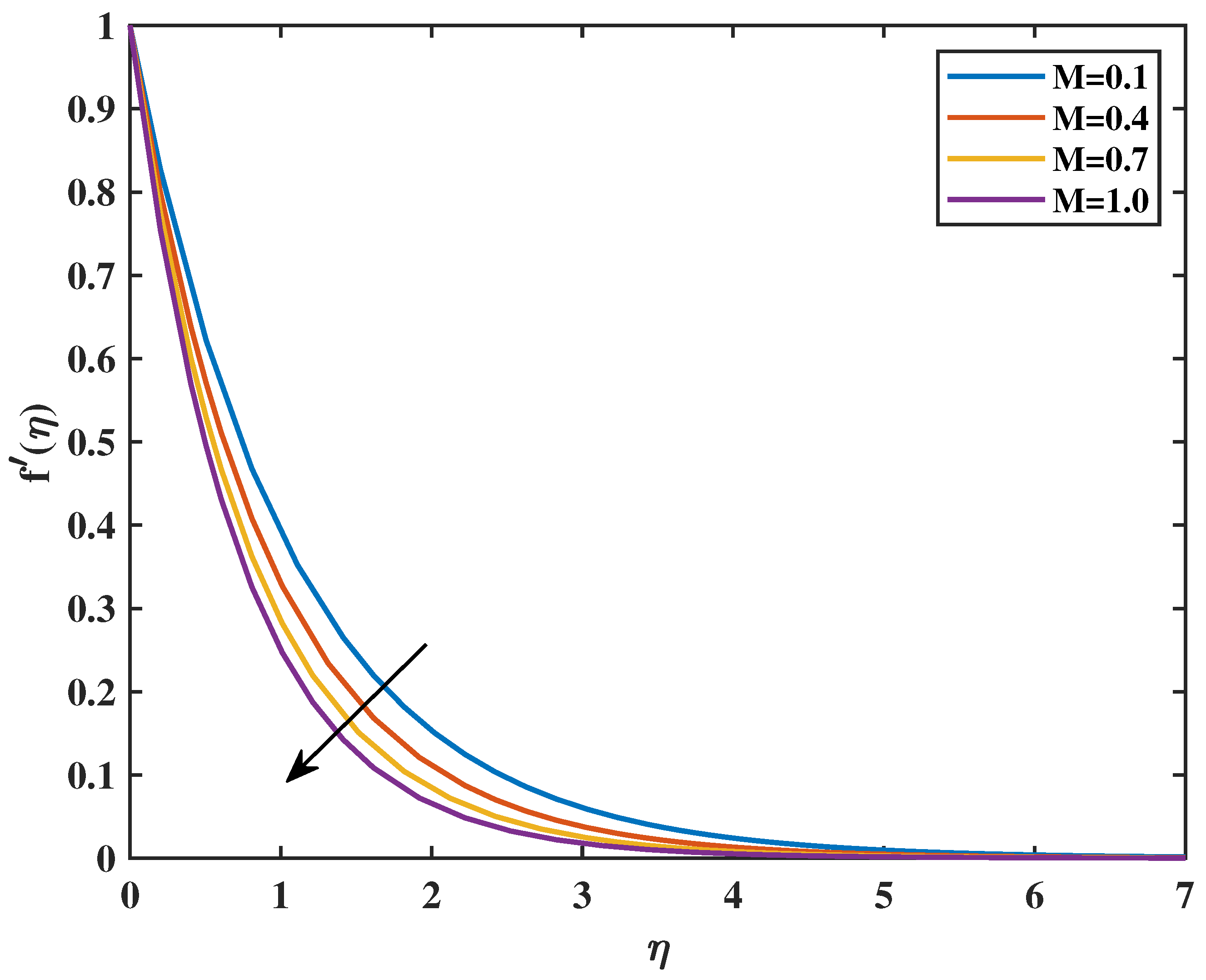
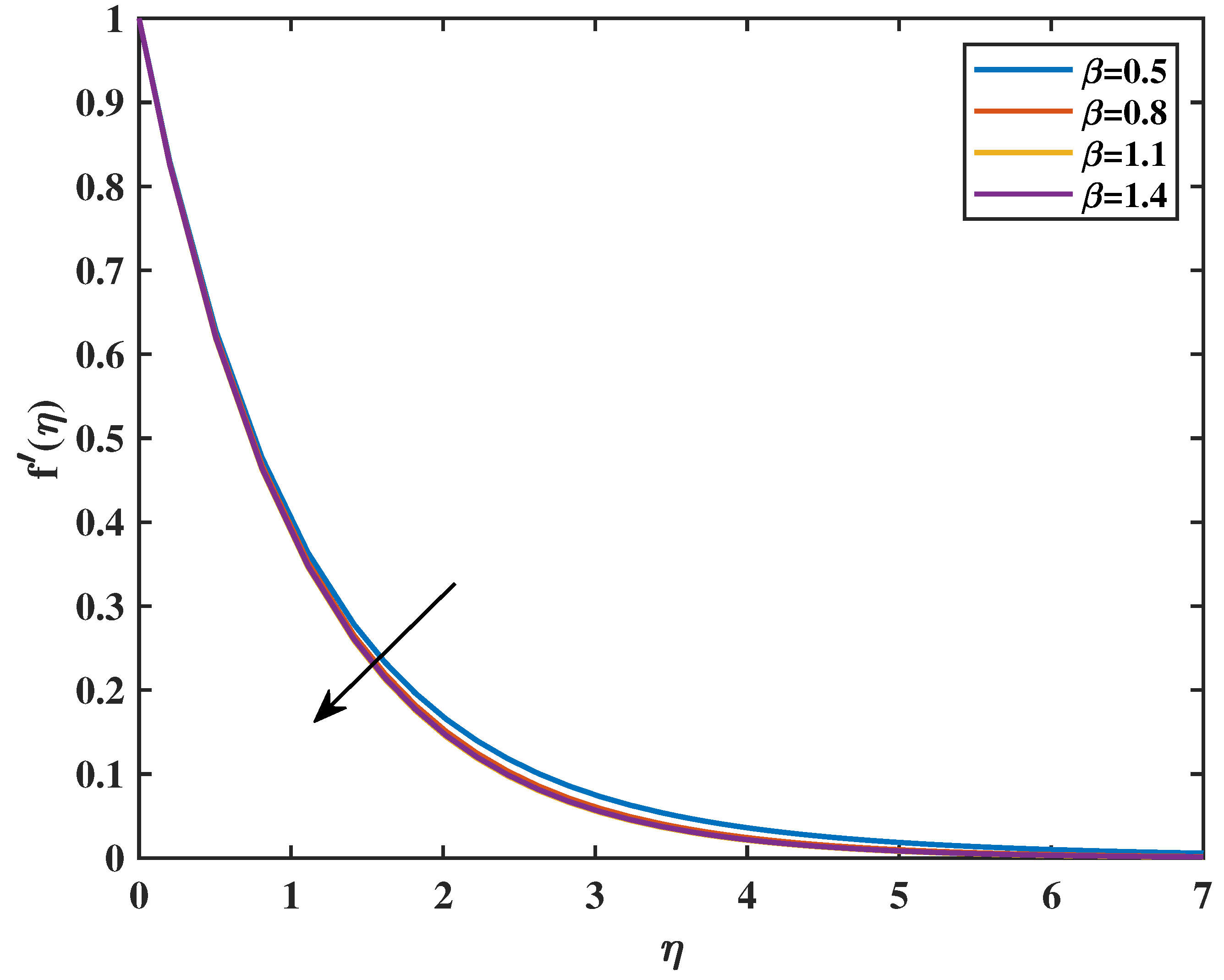
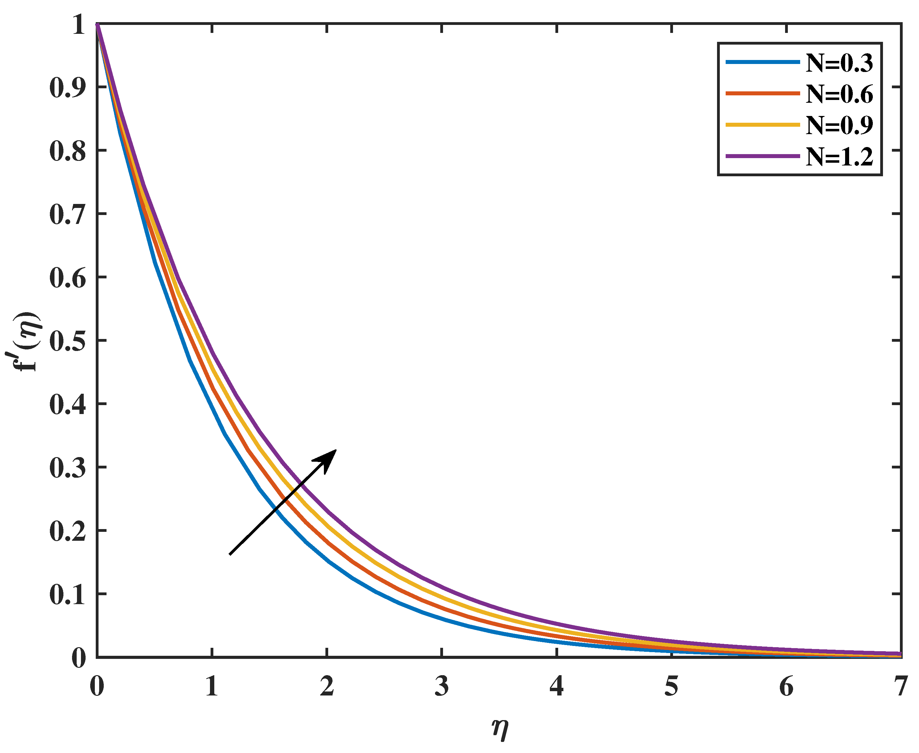
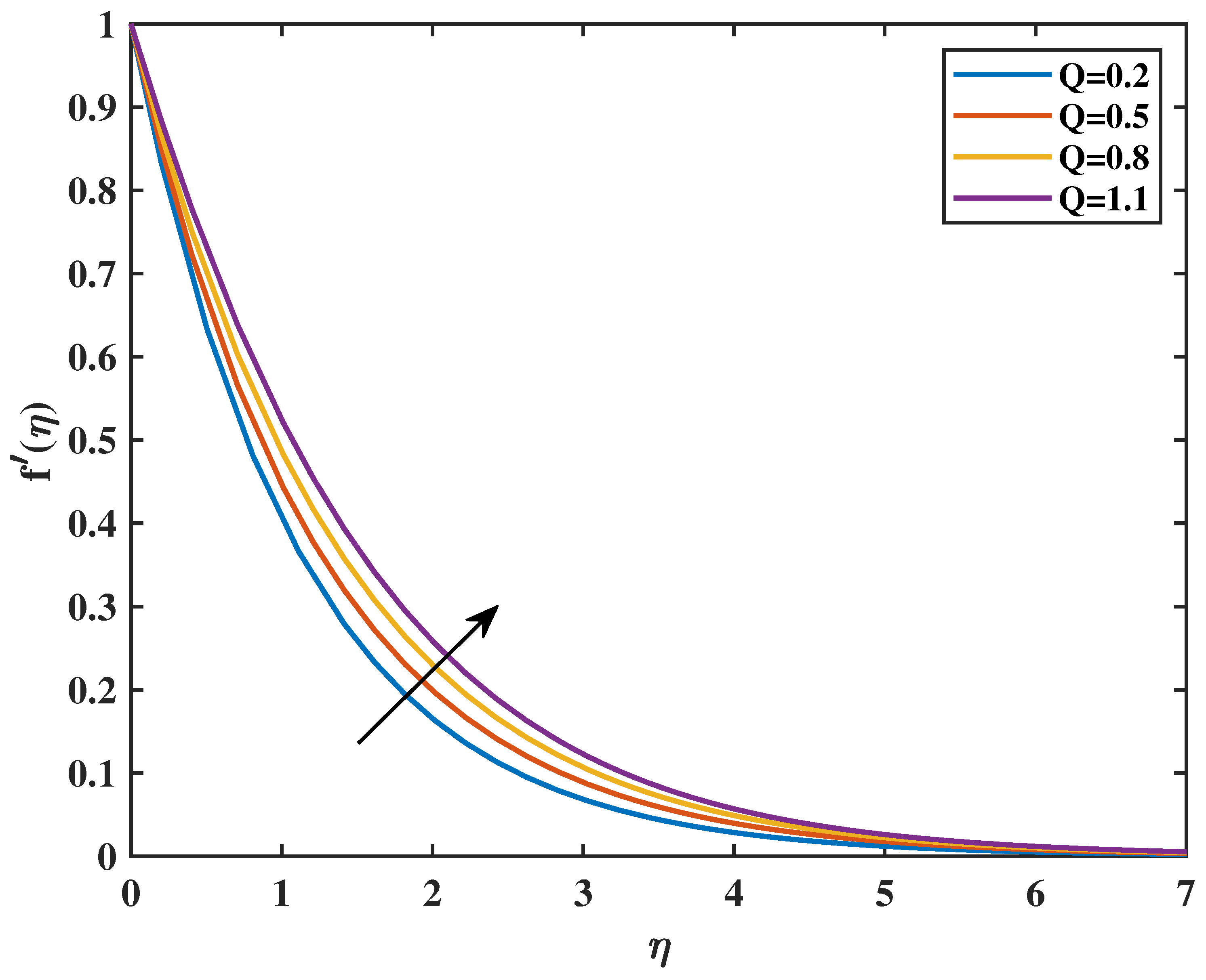
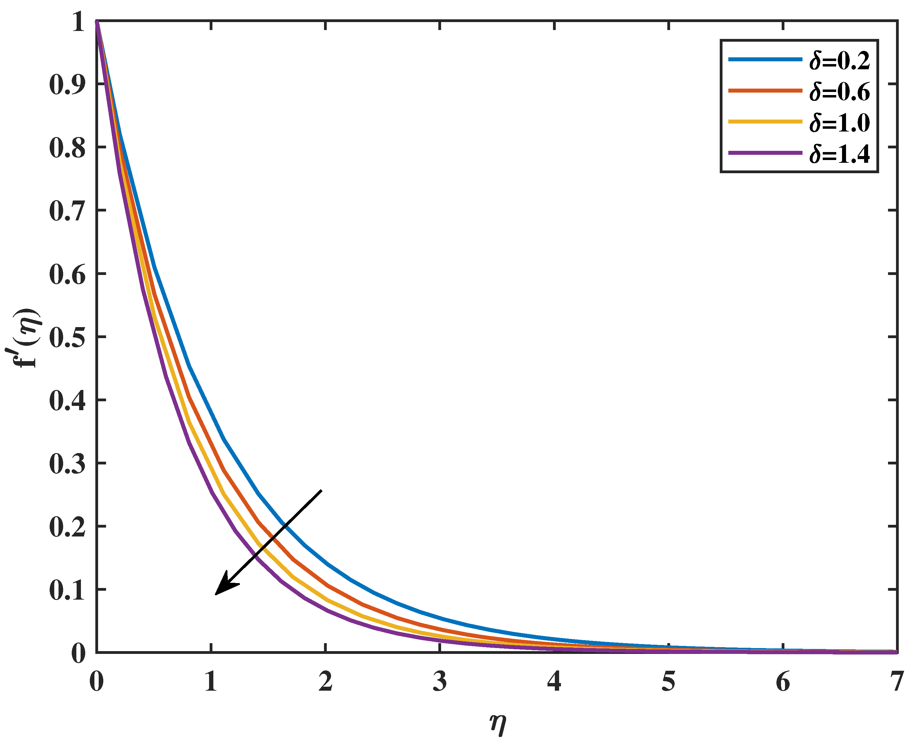
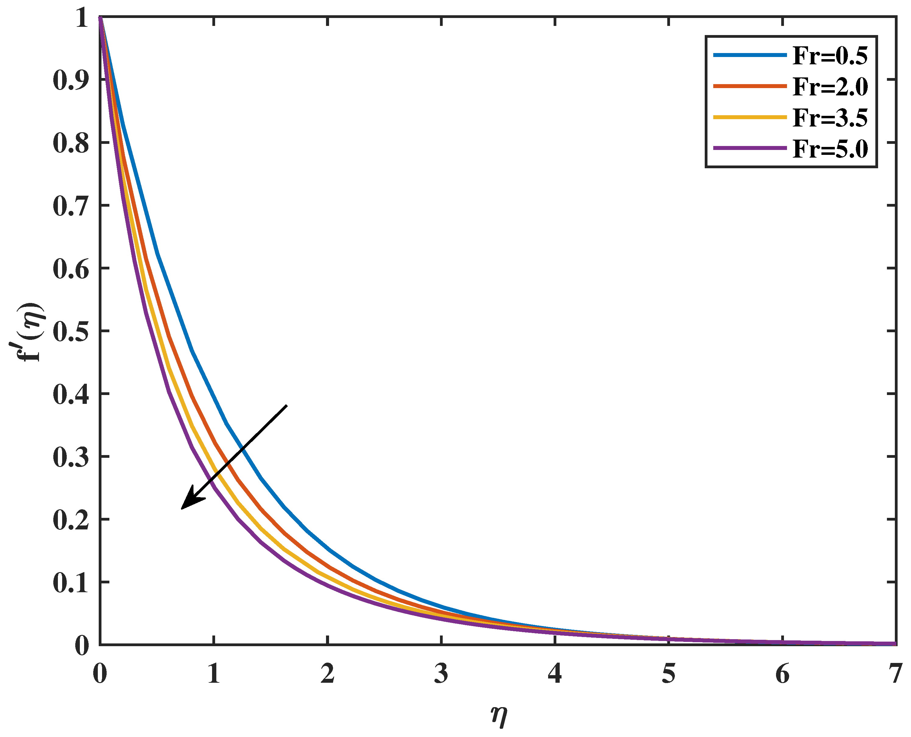
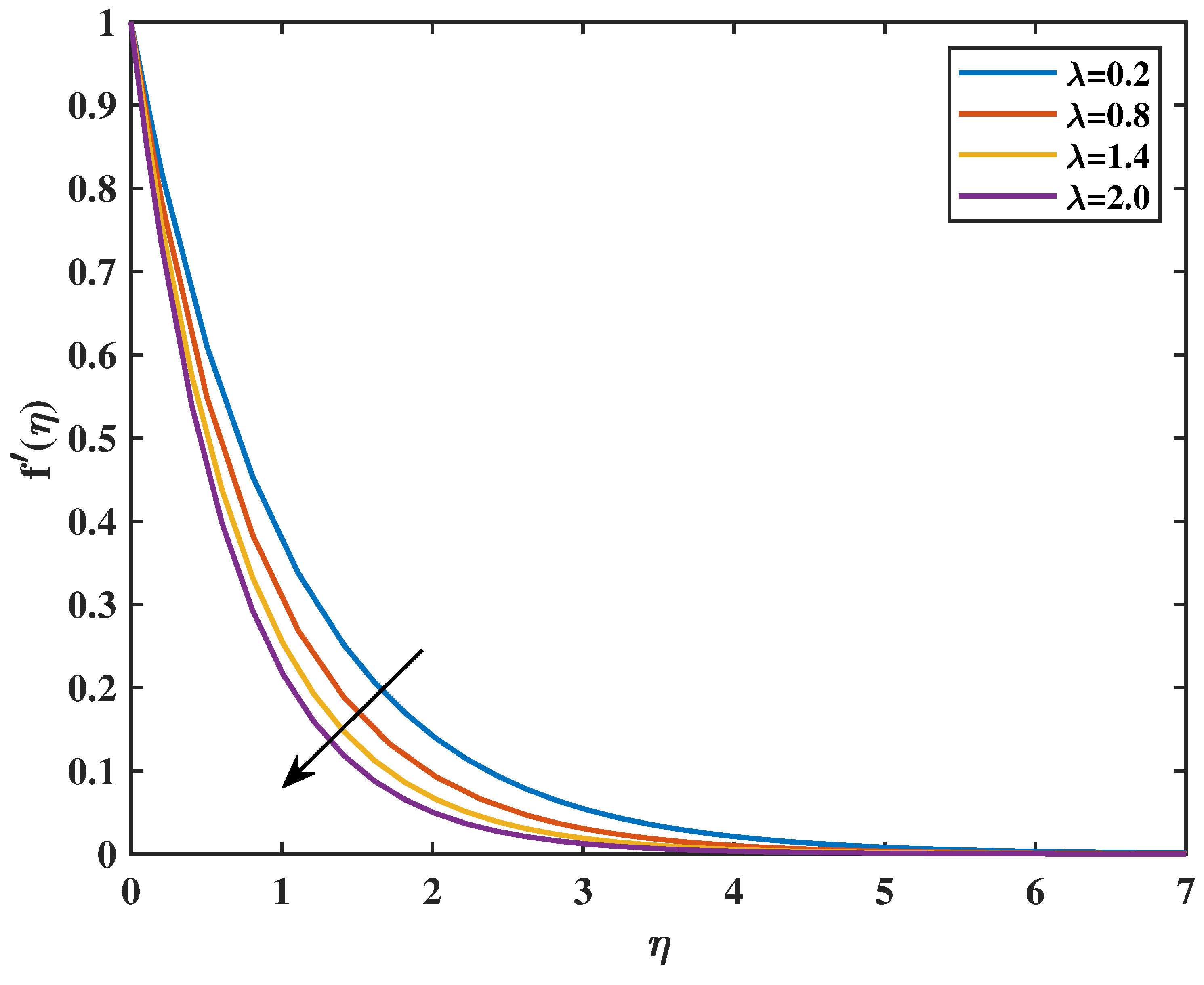
In Figure 2, the velocity profile as a function of the magnetic parameter (M) is exhibited. This proves that the velocity diminishes as the value of M increases. From a physical standpoint, the Lorentz forces that accompany the boundary layer for the magnetic field decrease as the value of M rises. The magnetic field, impeded by viscous forces and counteracting them, confines the fluid. Figure 3 shows the impacts of the dimensionless parameter β on velocity profiles. It shows that an increase in β causes a decrease in velocity f ( η ) . This is because fluid viscosity increases as the parameter β increases, resulting in a decrease in velocity. Figure 4 reveals that an increase in the value of the Powell–Eyring parameter (N) causes a rise in the value of velocity f ( η ) . It indicates that the Powell–Eyring parameter serves as a reflection of the activation energy required by fluid molecules to surpass intermolecular interactions and engage in flow under strain. A diminutive activation energy denotes reduced values of (N), thereby enabling the facilitation of molecular movement. Such an implication implies that velocity ascends with the increase in (N). Figure 5 shows that a higher value of the Hartmann number (Q) corresponds to a magnetic field that is more powerful relative to the viscous forces present in the flow of the fluid. Within MHD systems, a stronger magnetic field tends to exert a greater amount of force on the conductive fluid, which can potentially result in the fluid being restricted or confined to a specific direction. It is possible that a stronger magnetic field, as a result of a higher Q, could lead to modifications in the flow profiles within the conductive fluid. These modifications have the potential to result in increased fluid velocities. Figure 6 shows that an increase in the porosity parameter ( δ ) causes a reduction in velocity. The velocity profile’s relationship to the Forchheimer factor is seen in Figure 7. Physically, the inertial drag force is formed by increasing values of F r , which resists and causes the velocity ( f ( η ) ) curve to decrease. Figure 8 indicates that increasing the fluid parameter ( λ ) causes reduction in fluid velocity f ( η ) .

4.2. Temperature Profiles

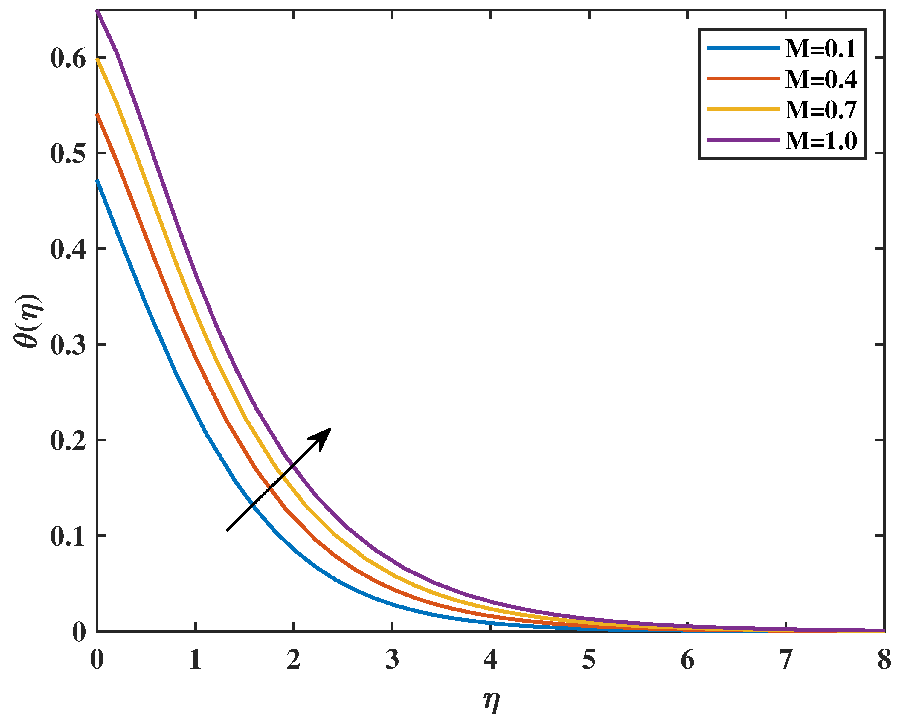
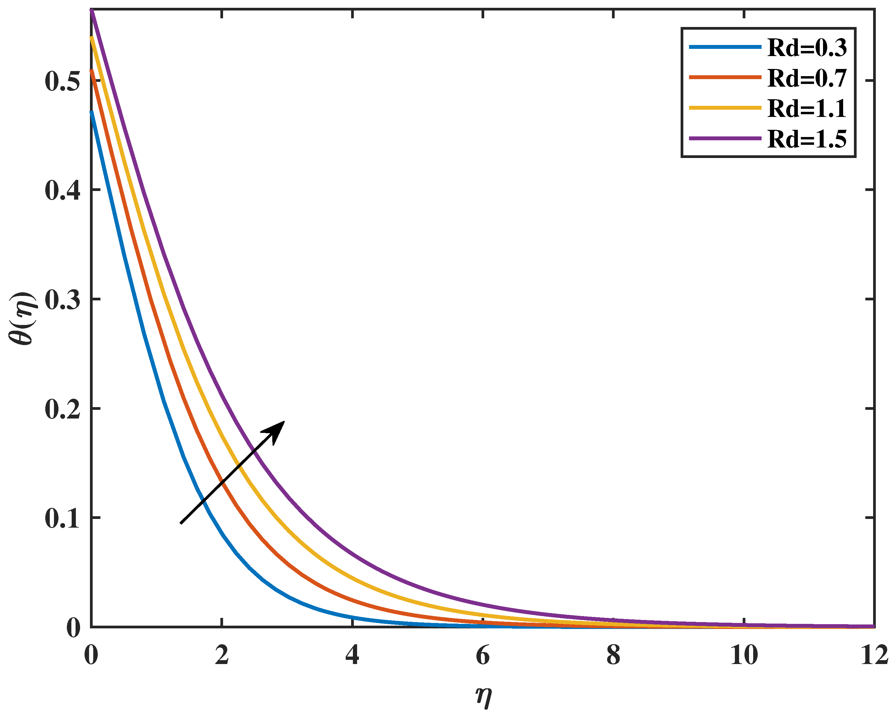
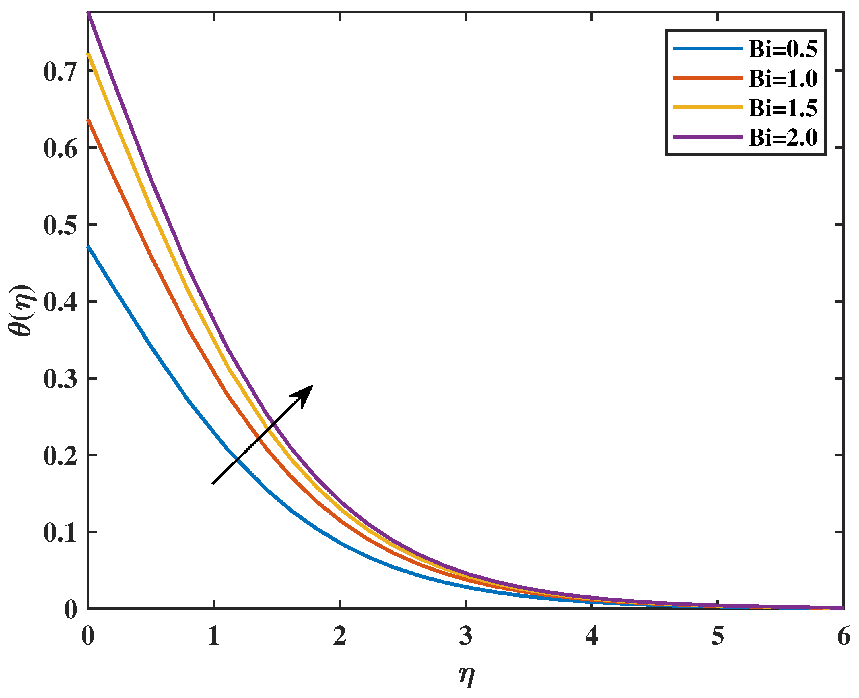
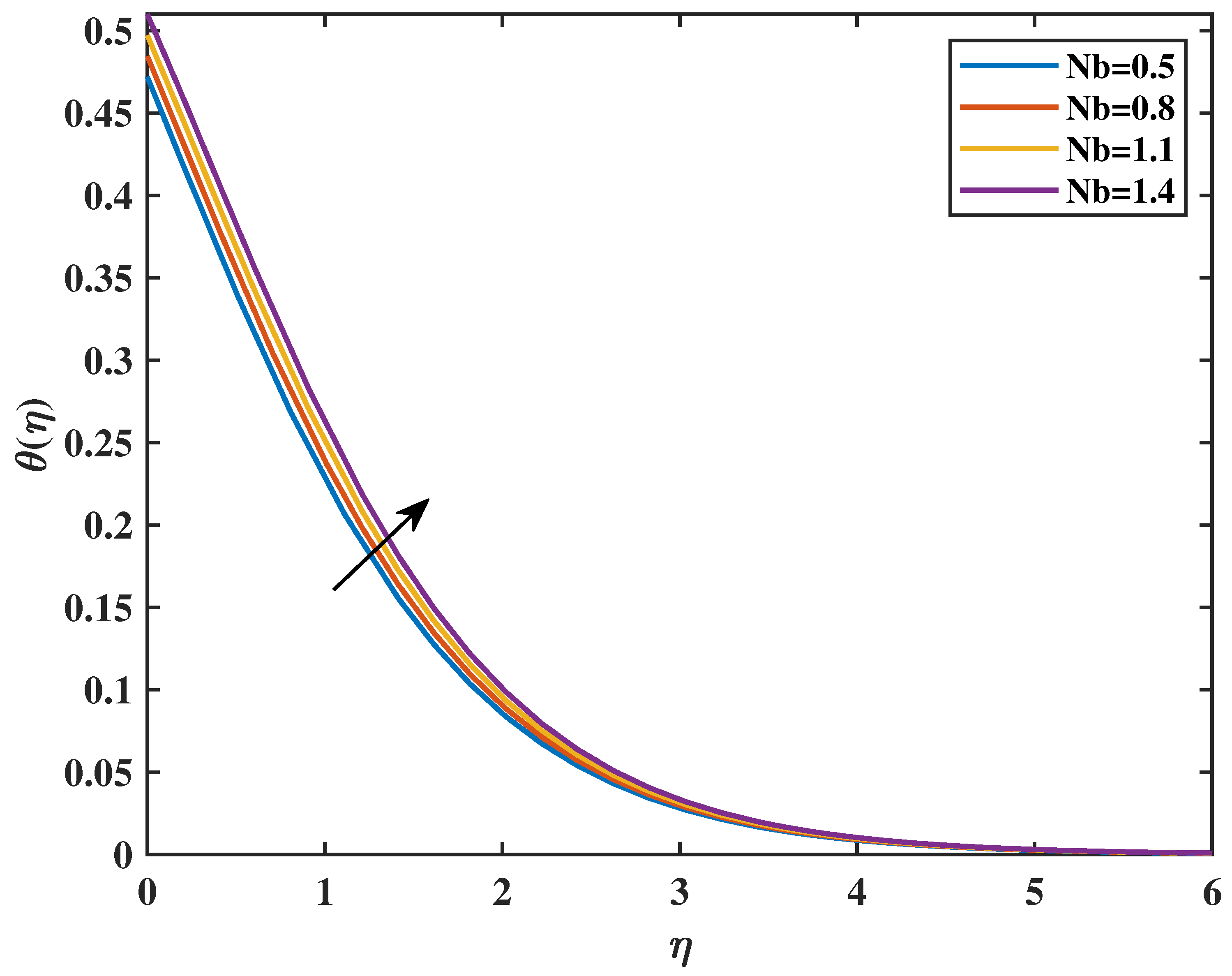
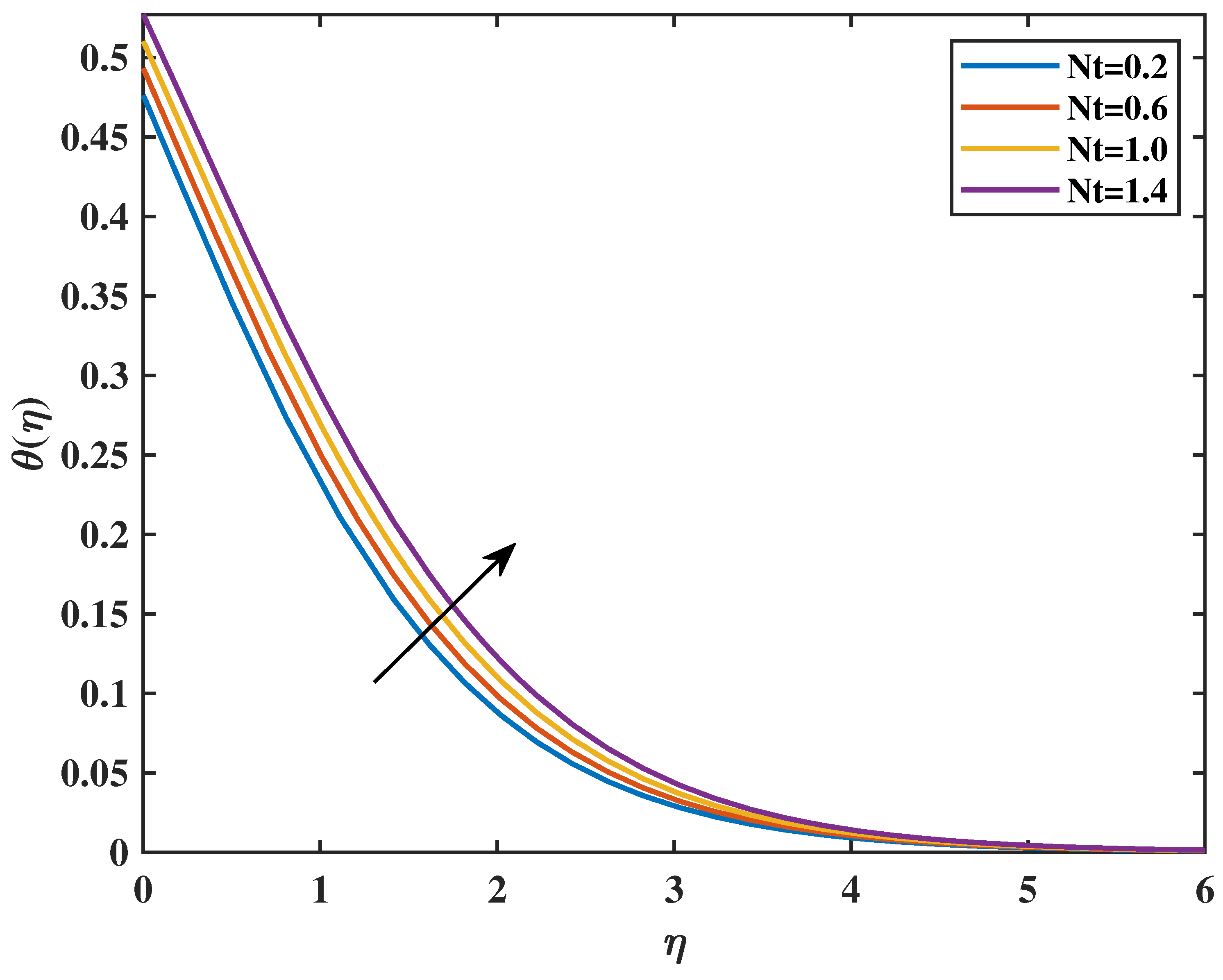
Figure 9 shows that increasing the value of the magnetic parameter (M) causes an increment in the value of the temperature profiles θ ( η ) . Figure 10 shows that higher values of the R d increase temperature profiles. Physically, for greater values of R d , more heat to the governing fluid gives an increase in boundary-layer thickness and temperature profiles. Figure 11 shows the effect of the thermal Biot number with temperature. Clearly, temperature is increased with an increase in values of B i . Actually, the thermal Biot number increases the thermal coefficient number. The features of the N b on temperature profiles are shown in Figure 12. The irregular and unpredictable movement of nanoparticles within nanofluids is commonly referred to as Brownian motion. Brownian motion of fluid at the molecular scale is a crucial element that affects the thermal conductivity of nanofluids. In fact, increasing Nb increases the kinetic energy of nanoparticles with which temperature is increased. The behavior of thermophoresis parameter ( N t ) is sketched in Figure 13. From the graph, it is clear that by increasing the value of ( N t ), the curve of temperature is enlarged. The larger value of Nt causes the intensification of the percentage of nanoparticles, resulting in an increase in temperature profiles θ ( η ) .

4.3. Concentration Profiles

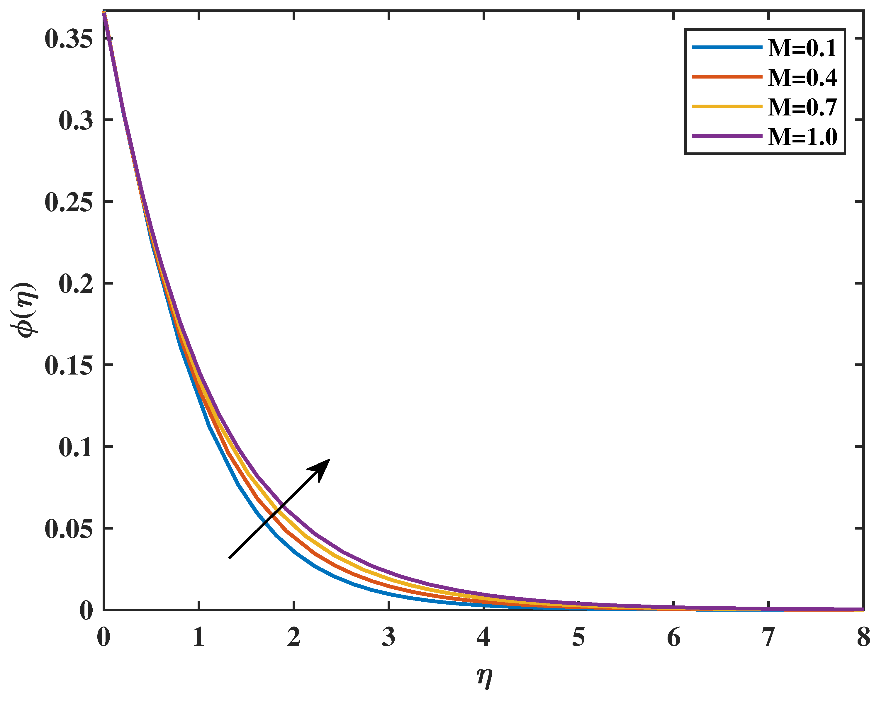
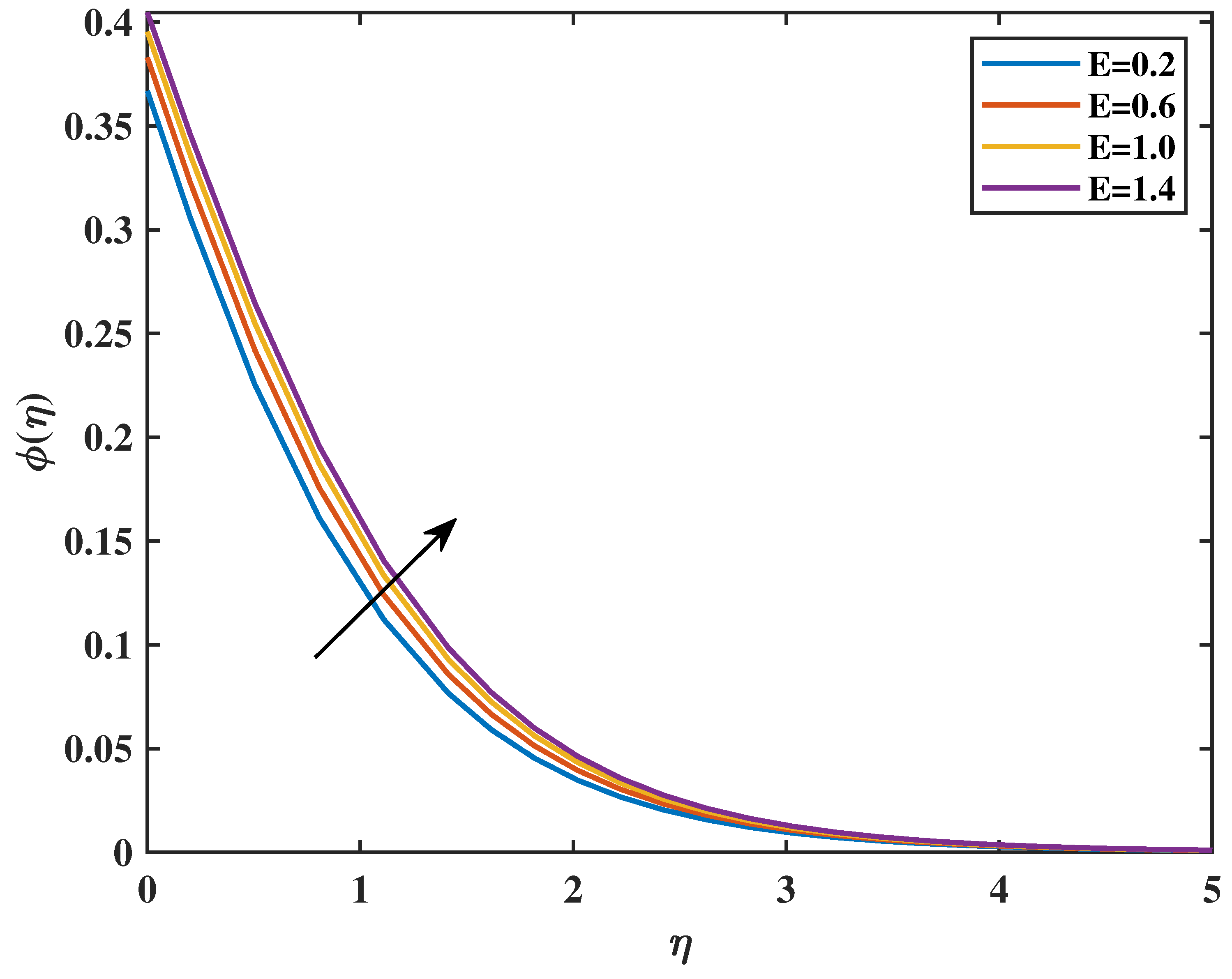
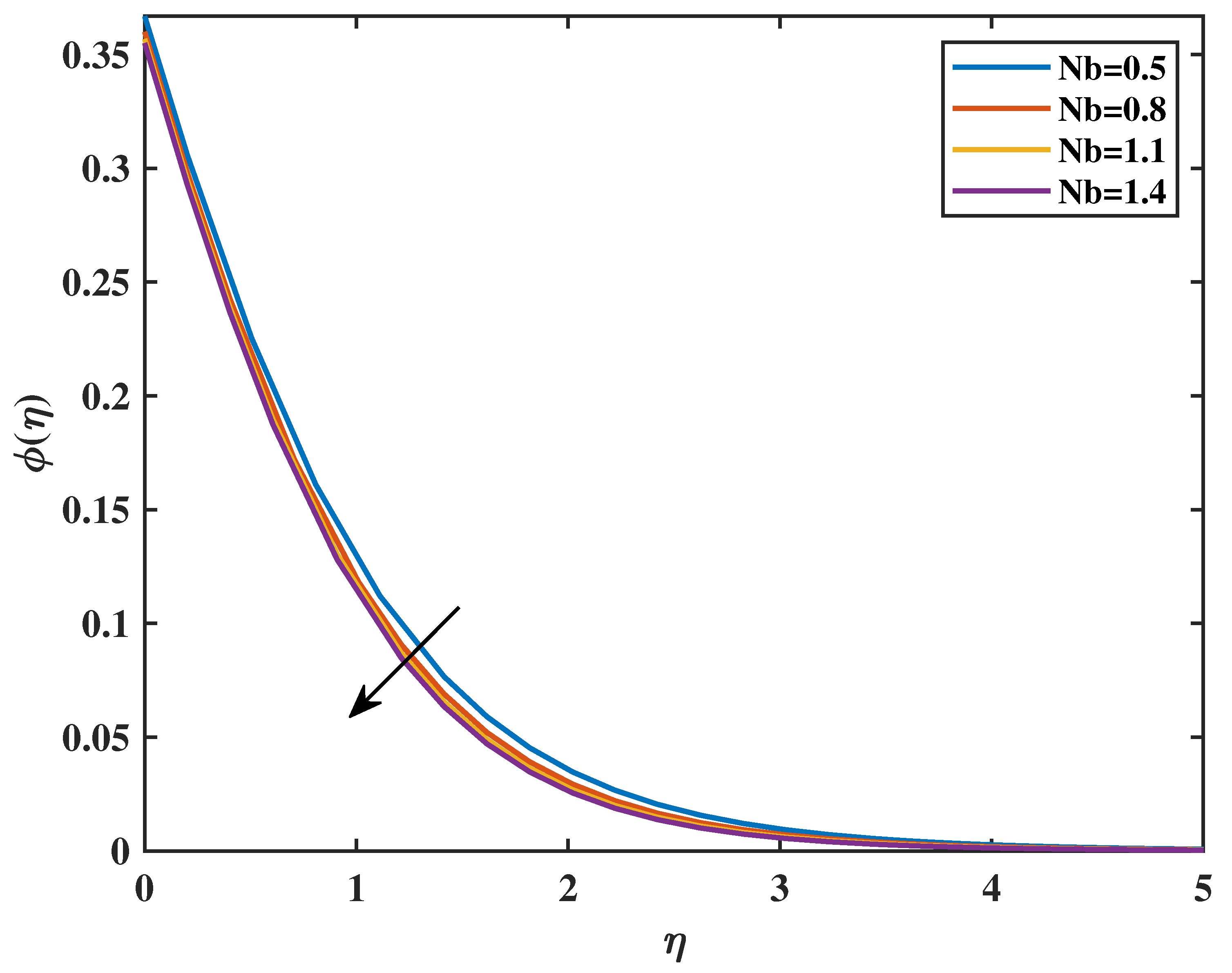
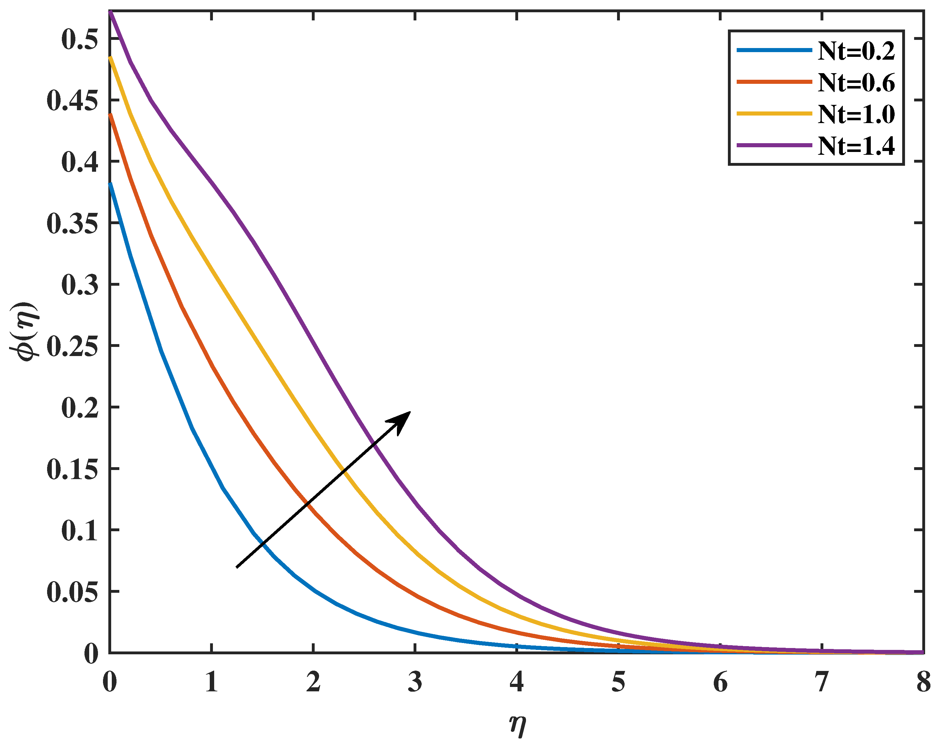
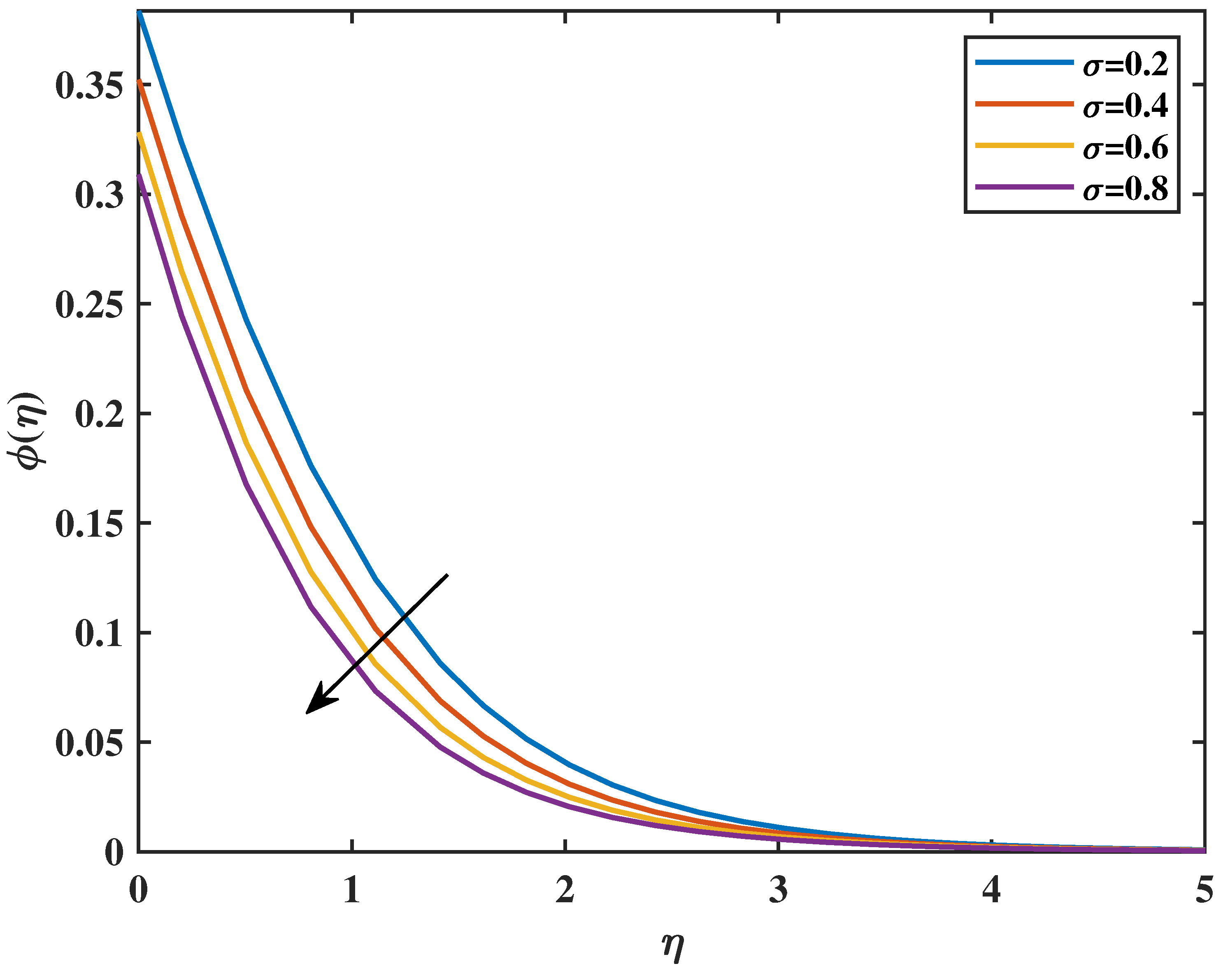
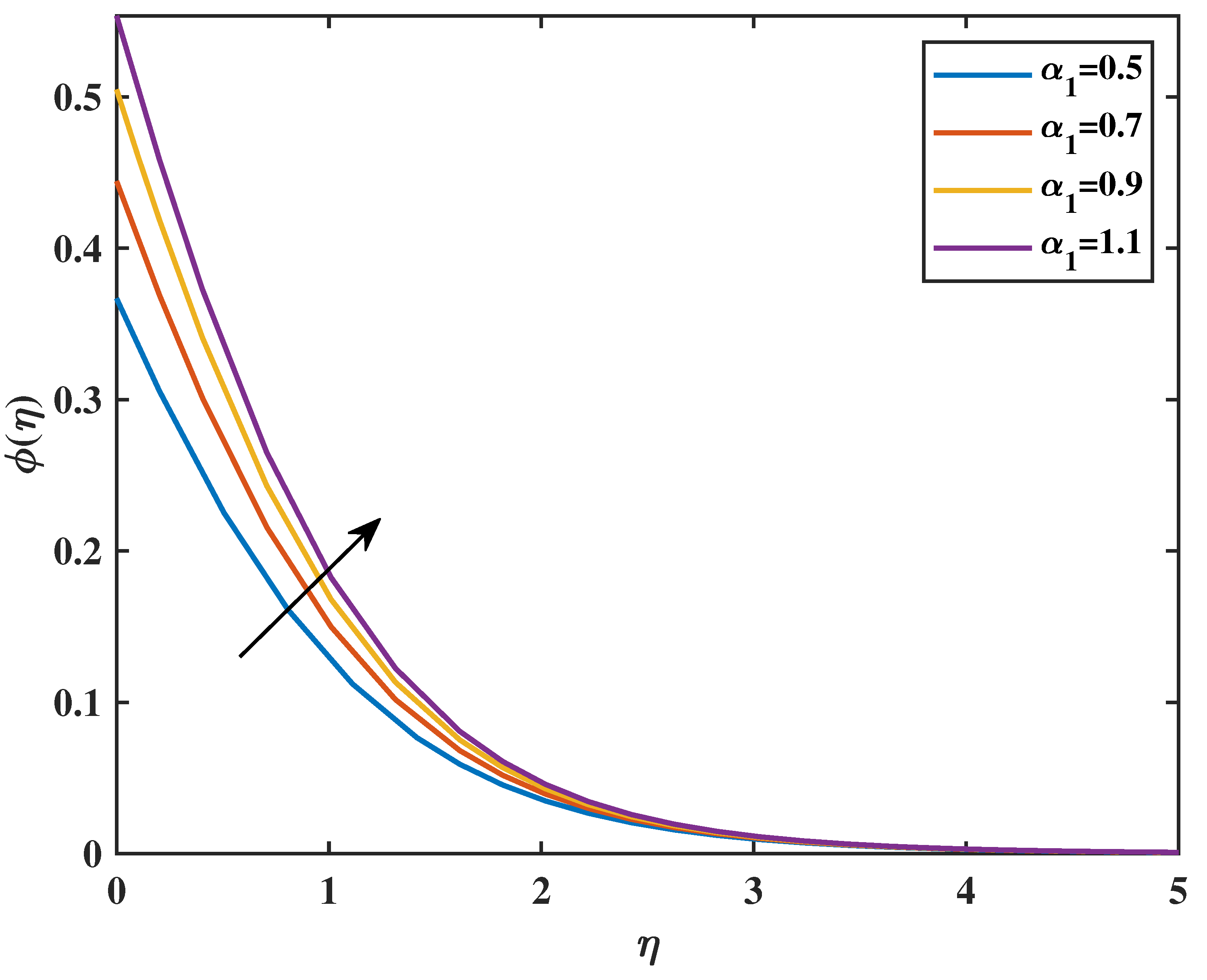
Figure 14 shows that for the rise in magnetic parameter, there is an increase in concentration profiles. In Figure 15, the relation between activation energy (E) and concentration profile ϕ ( η ) is analyzed. For larger values of activation energy (E), there is a rise in concentration ϕ ( η ) of nanoparticles in nanofluid. The effect of N b on concentration profile ϕ ( η ) is discussed in Figure 16. This figure demonstrates how the concentration profile is lowered with an increase in N b . This is because an increase in Brownian motion enhances random motion, which disperses the particles; hence, concentration decreases. The consequences of thermophoresis parameter ( N t ) for concentration profiles are discussed in Figure 17. The reduction in thermophoretic parameter values results in an elevation in the concentration profile. Thermophoresis induces a suction-like effect between the particles, resulting in surface cooling and a subsequent decrease in mass transfer. A noticeable deviation in the slope of the concentration curve ϕ ( η ) occurs within the interval 1 < η < 2 . This irregularity arises due to the strengthened thermophoretic influence in the near-wall region, where the competition between molecular diffusion and thermophoretic transport becomes more pronounced, leading to a brief enhancement in particle movement before the profile gradually levels off farther from the wall. Figure 18 illustrates how the behavior of the distribution of nanoparticle concentration changes as the reaction rate constant changes. As expected, an increment in the parameter of chemical reaction ( σ > 0 ) is accompanied by a drop in the concentration profile. Figure 19 illustrates the variation in concentration with change in concentration slip parameter ( α 1 ). In this, it is observed that the concentration profiles of nanoparticles is enhanced as the concentration slip parameter increases.

4.4. Other Physical Quantities

The variations in the Nusselt number and skin friction coefficient for nanofluid flow at different dimensionless parameter values are shown in Table 1 and Table 2, respectively. For larger inputs of the magnetic parameter M, σ , and the Darcy–Forchheimer parameter F r , the skin friction coefficient of the Powell–Eyring nanofluid flow increased; however, when the values of N and Q rose, it dropped. For larger inputs of M , N t , and N b , the Nusselt number of the Powell–Eyring nanofluid flow exhibited diminishing behavior, whereas at higher values of R d and B i , it exhibited increasing behavior.

5. Artificial Neural Network Analysis

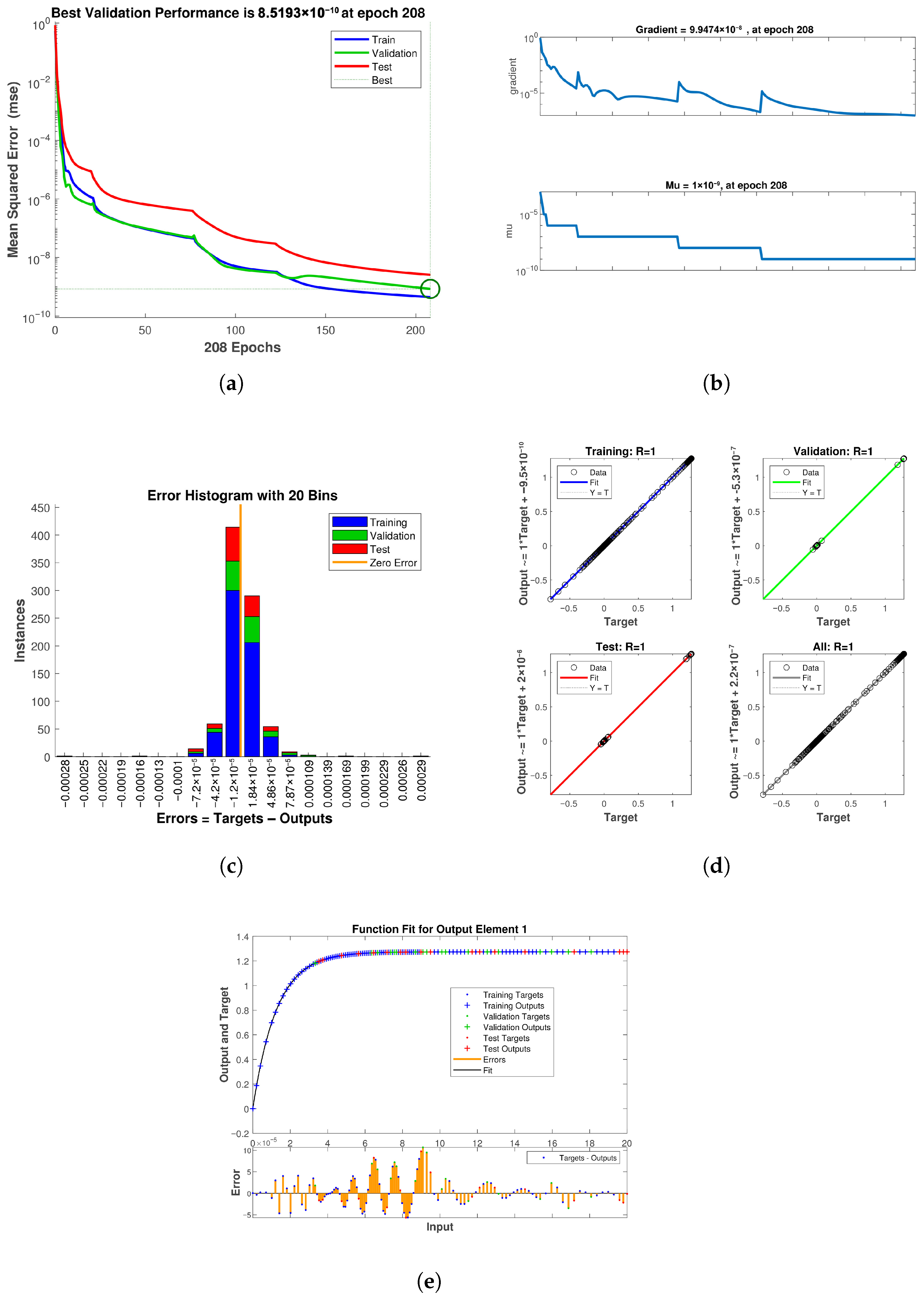
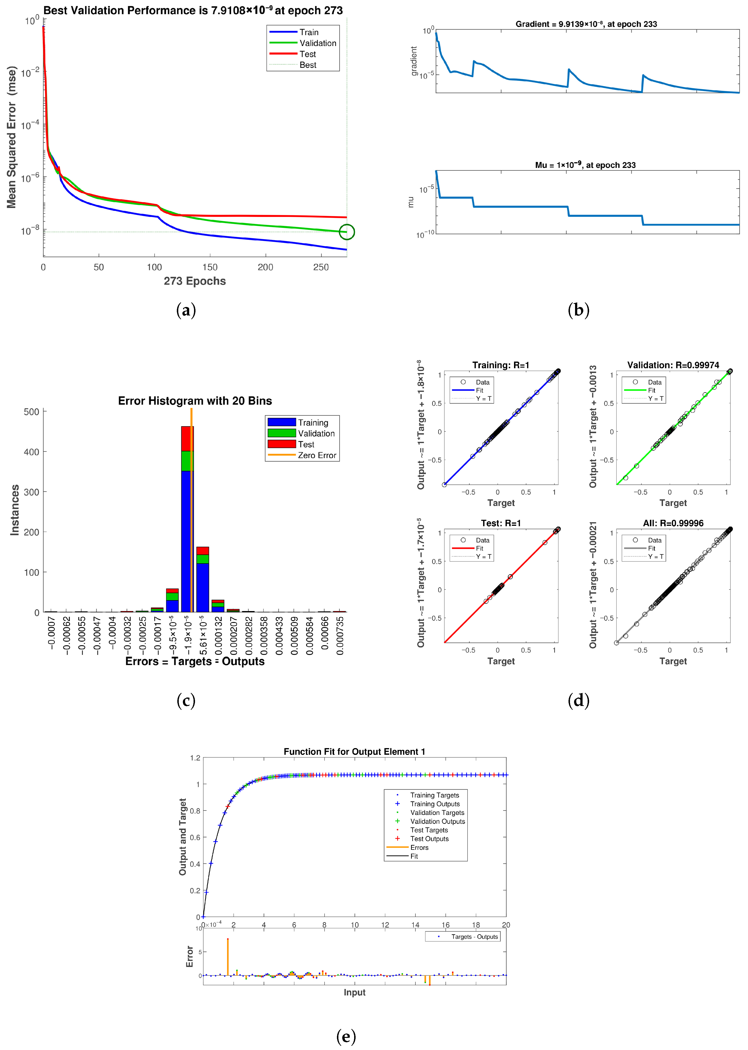
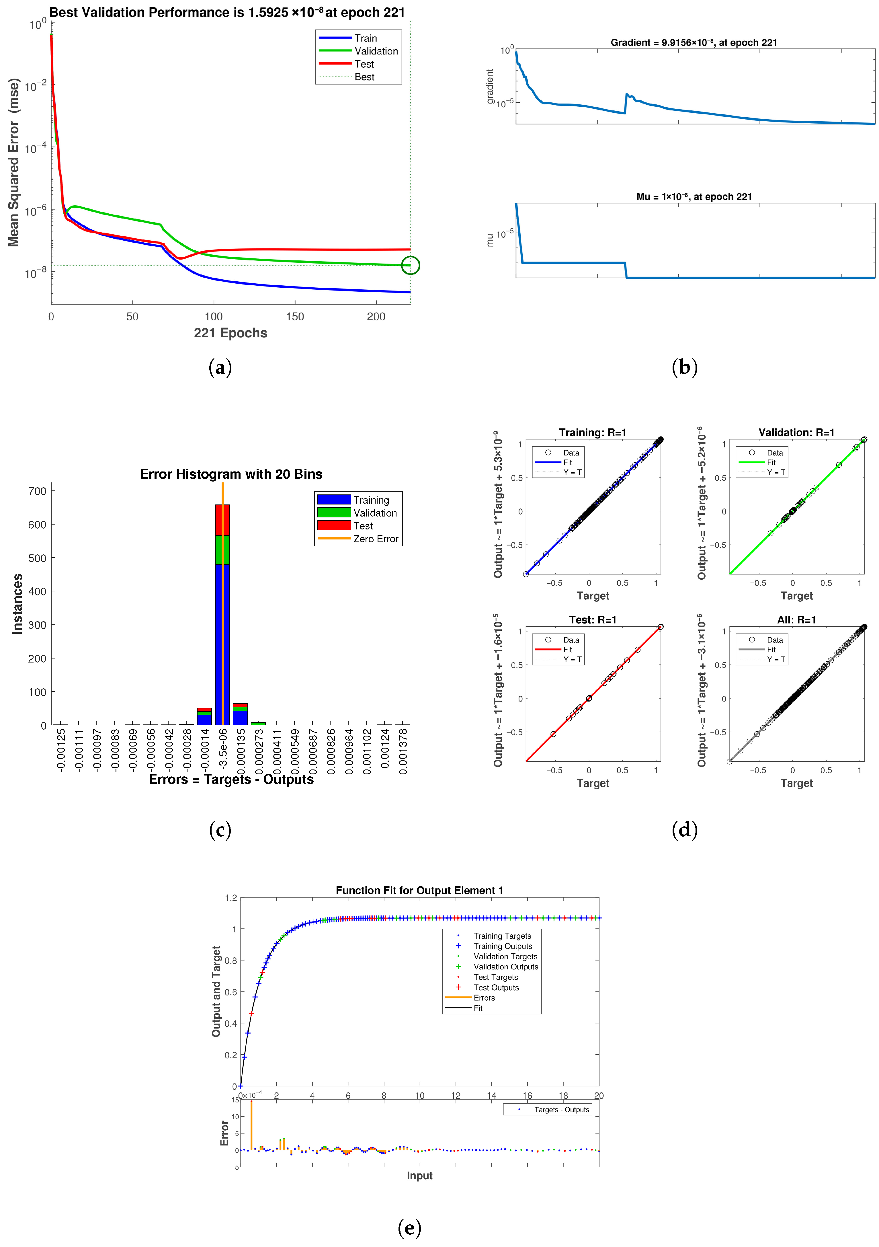
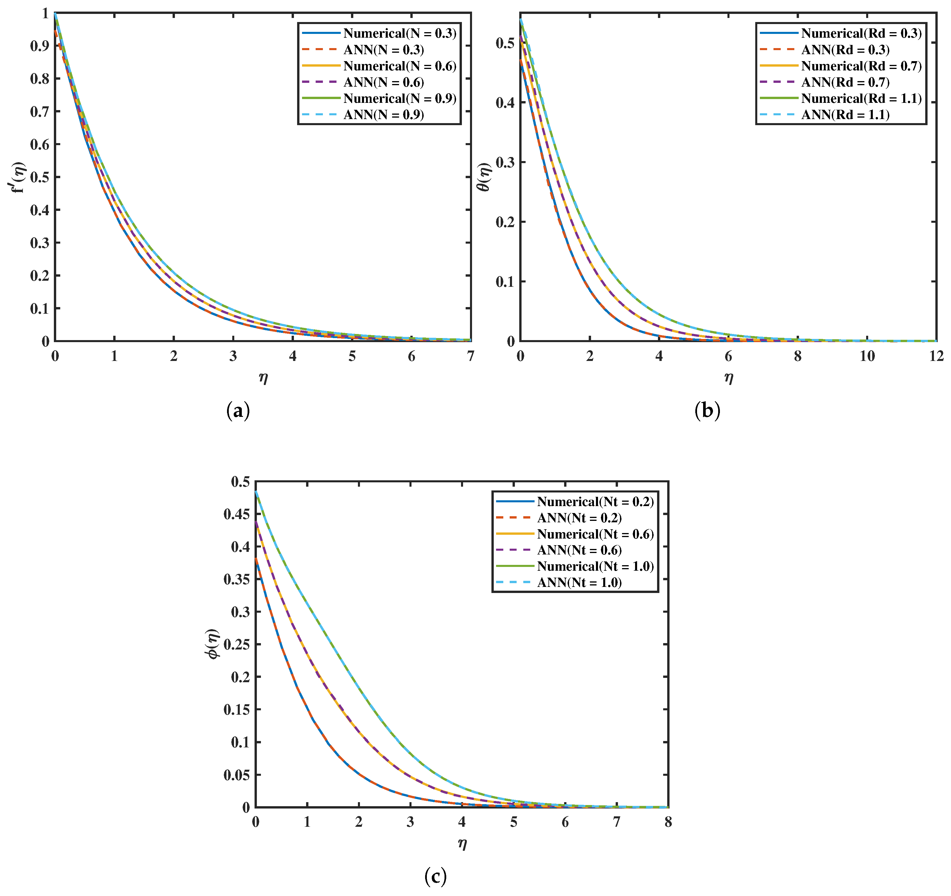
Artificial neural networks represent computational architectures that draw inspiration from the functional dynamics of the human brain. ANNs are constructed upon simulated neuronal elements that are interconnected through diverse configurations to establish a network. Analogous to the human brain, ANNs can learn, retain information, and establish associations among data that may initially appear disordered. Progressions in computational capabilities have facilitated the deployment of ANNs in addressing pragmatic challenges in various domains. The ANN constitutes a prominent example of nonlinear computational methodologies that endeavor to emulate the human neural architecture [33,34]. ANN frameworks possess the capability to effectively analyze and forecast intricate nonlinear process parameters through the utilization of approximation functions. The field of modeling has witnessed a significant surge of interest in ANNs, attributable to their advantageous properties as a robust technique proficient in learning complex and nonlinear processes [35]. Motivated by the complex structure of the human brain, ANNs have become a potent computational paradigm that can mimic cognitive processes including learning, categorization, prediction, generalization, and data grouping. ANNs handle difficult tasks with comparable efficiency by imitating the evolutionary patterns of neural processing. The development of various network topologies is made possible by advancements in training algorithms and the configuration of inter-neuronal connections, which are typically organized into three fundamental layers: input, hidden, and output. The hybrid computational framework used in this study combines Mathematica and MATLAB to construct and train ANN models. First, numerical datasets are generated using MATLAB’s neural network toolbox, and these are used for training. The ANN-LMA approach is a very effective substitute for skillfully handling the complexities of our research, as it exhibits commendable efficacy in the realm of nonlinear optimization challenges [36]. Thirteen neurons make up the first layer, and there are fourteen neurons in the second layer. Additionally, the network is trained for 3000 epochs. A rapid surrogate for the numerical solver was constructed using a feed-forward ANN with two hidden layers (13 and 14 neurons) trained using the Levenberg–Marquardt method and training data produced from high-accuracy simulations. The network exhibited outstanding prediction accuracy, with best validation MSEs of 8.52 × 10 10 for the Powell–Eyring parameter model, 7.91 × 10 9 for the thermal radiation model, and 1.59 × 10 8 for the thermophoresis model, obtained at epochs 208, 273, and 221, respectively. Across training, validation, and testing, regression graphs displayed R values ranging from 0.9997 to 1.0000, and error histograms were symmetric about zero with little dispersion, suggesting unbiased predictions. The ANN was found to accurately represent temperature profiles for various radiation parameters R d , which reflect enhanced radiative heating and thermal-layer thickening; concentration profiles for thermophoresis parameters N t , which show particle redistribution consistent with stronger thermophoretic forces; and velocity profiles for varying Powell–Eyring parameters N, which capture the rise in near-wall velocity with higher N. These results were verified by comparisons using numerical solutions. Small deviations only happened in distant areas with little real-world significance. An effective tool for quick parametric research, optimization, and real-time applications in MHD nanofluid heat transfer issues, the ANN generated predictions nearly instantaneously after training. Figure 20 shows the ANN training results for the Powell–Eyring parameter case. The mean squared error decreases rapidly with increasing epochs and stabilizes at a very small value, reflecting excellent learning efficiency. The training states confirm smooth convergence without instability, while the error histogram is narrow and centered around zero, highlighting minimal and unbiased errors. The regression plot indicates R 1.0 , which confirms that the ANN predictions are almost identical to the numerical targets. Figure 21 illustrates the ANN performance for the thermal radiation parameter. The best validation error is achieved within a few hundred epochs, indicating that the network converged quickly. The gradient and training state curves remain stable, showing no overfitting or divergence. The error histogram is symmetric about zero, suggesting that the prediction errors are evenly distributed. Regression plots again display a correlation coefficient very close to unity, confirming strong agreement between ANN outputs and reference data. Figure 22 presents the ANN training for the thermophoresis parameter. The mean squared error curve shows rapid reduction and reaches an extremely small value, verifying that the network captured the thermophoretic influence accurately. The error histogram demonstrates that most errors are clustered very close to zero, while regression plots confirm almost perfect alignment between predicted and target values across training, validation, and testing datasets. This reflects the robustness of the ANN in modeling nonlinear thermophoretic effects. Figure 23 summarizes the overall ANN validation through comparative function-fit plots. The predicted profiles for velocity, temperature, and concentration closely follow the numerical results across the domain, with only negligible deviations in far-field regions where the gradients are weak. The overlap between target and output curves illustrates that the ANN generalizes well beyond training data, making it a reliable surrogate model for quick parametric evaluations of the nanofluid system. Table 3 provides an overview of the ANN-LMA training conducted in this study.

6. Conclusions

A numerical investigation is carried out to examine the combined impacts of thermal radiation, activation energy, and Darcy–Forchheimer resistance on Powell–Eyring nanofluid motion in a porous medium interacting with a Riga plate. The problem is mathematically formulated using the Buongiorno model. Nonlinear PDEs are transformed into ODEs via similarity adjustments. MATLAB BVP4C is utilized to acquire the final outcomes. The only purpose of the Mathematica/NDSolve ANN datasets is to train surrogate models. Additionally, tables for skin friction and Nusselt numbers against various parameters are obtained. The outcomes of the current research are as follows:
  • Our computations show that increasing M slows the flow and reduces local heat transfer, while increasing Q may produce a local near-wall acceleration and modify the heat-transfer distribution.
  • By increasing the inputs of magnetic parameter, porosity, fluid parameter, and Darcy–Forchheimer number, the velocity profiles declines.
  • The wall-parallel electromagnetic force created by the Riga parameter Q locally increases the near-wall velocity.
  • The heat transfer is enhanced with rising values of the magnetic parameter, thermal radiation, Brownian motion, thermophoresis forces, and thermal Biot number.
  • The concentration curves are boosted for larger values of the magnetic parameter, activation energy, thermophoresis forces, and concentration Biot number.
  • An increase in the Brownian motion parameter and the chemical reaction parameter causes the concentration distributions to decline, reflecting enhanced particle diffusion and reactive consumption in the fluid.
  • The wall velocity drops by around 14% when the Hartmann number (M = (1.2) increases; the velocity is lowered by about 11% when the Forchheimer drag increases by 0.2; and the heat transfer rate rises by about 9% when the Biot number climbs from 0.1 to 0.3.
  • The skin friction coefficient of Powell–Eyring nanofluid flow is enhanced by higher inputs of magnetic parameter M and the σ Darcy–Forchheimer parameter F r , while it declines with the increasing values of N and Q.
  • For larger inputs of M , N t , and N b , the Nusselt number of the Powell–Eyring nanofluid flow exhibits diminishing behavior, whereas higher values of R d and B i cause it to exhibit increasing behavior.
Additional analysis highlights three notable physical behaviors emerging from the present investigation:
  • Variations in fluid viscosity together with Darcy–Forchheimer drag markedly affect the momentum transport. An intensified Darcy–Forchheimer resistance acts as an additional inertial barrier, thereby lowering the fluid motion across the porous matrix.
  • The interplay between thermophoretic forces and chemical interaction modifies the species distribution. Stronger thermophoresis drives nanoparticles further from the wall, whereas elevated reaction intensity promotes concentration depletion near the surface.
  • Adjustments in permeability and radiative heat flux directly alter the thermal field. Enhanced radiation contributes to the growth of the thermal layer, while increasing porosity generally diminishes near-wall convection strength.

Author Contributions

Conceptualization, M.F.M. and S.A.A.S.; Methodology, Z.A. and A.R.A.; Validation, S.A.A.S.; Formal analysis, A.R.A. and S.A.A.S.; Investigation, Z.A.; Resources, A.R.A.; Data curation, M.F.M.; Writing—original draft, Z.A.; Writing—review & editing, Z.A. and M.F.M.; Supervision, S.A.A.S.; Project administration, M.F.M.; Funding acquisition, A.R.A. All authors have read and agreed to the published version of the manuscript.

Funding

This work was supported and funded by the Deanship of Scientific Research at Imam Mohammad Ibn Saud Islamic University (IMSIU) (grant number IMSIU-DDRSP2502).

Institutional Review Board Statement

The authors declare that there is no conflict with publication ethics.

Informed Consent Statement

The authors declare that there is no conflict with the publication of this paper.

Data Availability Statement

Data sharing does not apply to this article, as no datasets were generated or analyzed during the current study.

Conflicts of Interest

The authors declare no conflicts of interest.

Nomenclature

ρ n f     Nanofluid density (kg·m−3) σ ˜ Electrical conductivity (S·m−1)
QRiga plate forcing parameter (W·m−3) ( u ˜ , v ˜ ) Velocity components (m·s−1)
fDimensionless primary velocity P r Prandtl number
N u Nusselt number ( N , λ ) Fluid parameters
θ Dimensionless temperature ( x , y ) Cartesian coordinates (m)
α 1 Temperature Biot number ν n f Kinematic viscosity of nanofluid (m2·s−1)
T Temperature away from the surface (K) R d Radiation parameter
T ^ Non-dimensional temperature (K) S h        Sherwood number
k * Mean absorption coefficient j * Current density
C f Skin friction factorkPermeability of porous medium (m2)
T w Temperature at surface (K) η Dimensionless variable
ρ c p Heat capacity (J·kg−1·K−1) K n f Thermal conductivity of nanofluid (W·m−1·K−1)
F r Darcy–Forchheimer coefficient F 0 Inertial coefficient
EActivation energy (J·mol−1) σ * Chemical reaction variable
ϕ Dimensionless concentration a 1 Diameter of the magnets
mPower index of velocity N t Thermophoresis coefficient
k r Chemical reaction rate C Ambient concentration
R e ( x ) Reynolds number N b Brownian motion coefficient
h 1 Connective variable D ˜ T Diffusion variable
D ˜ B Brownian diffusion factor T m Mean fluid temperature
δ Porosity coefficient (s−1) ψ Stream function
nFitted rate constantKBoltzmann constant (J·K−1)
σ ˜ Electrical conductivity c p Specific heat (J·kg−1·K−1)
C ˜ Fluid ambient concentration C ˜ w Concentration at wall
E c Eckert number L e Lewis number
δ ˜ Temperature difference parameter B i Thermal Biot number
α 1 Concentration slip parameterMHartmann number

References

  1. Berman, N.S. Drag reduction by polymers. Annu. Rev. Fluid Mech. 1978, 10, 47–64. [Google Scholar] [CrossRef]
  2. Guo, T.; Xiao, Z.; Sui, Y.; Huang, B.; Fu, C.; Yao, L. Optimization of gas–liquid two-phase flow law and structural parameters of Laval supersonic atomizing nozzle. Phys. Fluids 2025, 37, 073396. [Google Scholar]
  3. Masuda, H.; Ebata, A.; Teramae, K.; Hishinuma, N. Alteration of Thermal Conductivity and Viscosity of Liquid by Dispersing Ultra-Fine Particles, Dispersion of Al2O3, SiO2, and TiO2 Ultra-Fine Particles. Netsu Bussei 1993, 7, 227–233. [Google Scholar]
  4. Choi, S.U.; Eastman, J.A. Enhancing Thermal Conductivity of Fluids with Nanoparticles (No. ANL/MSD/CP-84938; CONF-951135-29); Argonne National Lab (ANL): Argonne, IL, USA, 1995. [Google Scholar]
  5. Eastman, J.A.; Choi, S.U.S.; Li, S.; Yu, W.; Thompson, L.J. Anomalously increased effective thermal conductivities of ethylene glycol-based nanofluids containing copper nanoparticles. Appl. Phys. Lett. 2001, 78, 718–720. [Google Scholar] [CrossRef]
  6. Awais, M.; Ullah, N.; Ahmad, J.; Sikandar, F.; Ehsan, M.M.; Salehin, S.; Bhuiyan, A.A. Heat transfer and pressure drop performance of Nanofluid: A state-of-the-art review. Int. J. Thermofluids 2021, 9, 100065. [Google Scholar] [CrossRef]
  7. Yaseen, N.; Shatat, F.; Alwawi, F.A.; Swalmeh, M.Z.; Kausar, M.S.; Sulaiman, I.M. Using micropolar nanofluid under a magnetic field to enhance natural convective heat transfer around a spherical body. J. Adv. Res. Fluid Mech. Therm. Sci. 2022, 96, 179–193. [Google Scholar] [CrossRef]
  8. Wu, J.; Lin, J.; Yan, Y.; You, Z.; Su, Z.; Long, J. Grooved-porous composite wick structures for highly efficient capillary-fed boiling heat transfer. Appl. Therm. Eng. 2024, 256, 124029. [Google Scholar] [CrossRef]
  9. Buongiorno, J. Convective transport in nanofluids. ASME J. Heat Mass Transf. 2006, 128, 240–250. [Google Scholar] [CrossRef]
  10. Owhaib, W.; Al-Kouz, W. Three-dimensional numerical analysis of flow and heat transfer of bi-directional stretched nanofluid film exposed to an exponential heat generation using modified Buongiorno model. Sci. Rep. 2022, 12, 10060. [Google Scholar]
  11. Wang, F.; Saeed, A.M.; Puneeth, V.; Shah, N.A.; Anwar, M.S.; Geudri, K.; Eldin, S.M. Heat and mass transfer of Ag–H2O nano-thin film flowing over a porous medium: A modified Buongiorno’s model. Chin. J. Phys. 2023, 84, 330–342. [Google Scholar] [CrossRef]
  12. Sindhu, S.; Sowmya, G.; Ramesh, N.L.; Gireesha, B.J. Heat transport analysis of nanoliquid in a microchannel with aggregation kinematics: A modified Buongiorno model approach. Int. J. Model. Simul. 2024, 1–21. [Google Scholar] [CrossRef]
  13. Zhu, X.; Zuo, Z.; Wang, W.; Jia, B.; Liu, R.; Yin, Q.; Zhang, M. Performance comparison and optimization of thermoelectric generator systems with/without stepped-configuration. Energy 2025, 335, 137924. [Google Scholar] [CrossRef]
  14. Zarei, A.; Karimipour, A.; Isfahani, A.H.M.; Tian, Z. Improve the performance of lattice Boltzmann method for a porous nanoscale transient flow by provide a new modified relaxation time equation. Phys. A Stat. Mech. Appl. 2019, 535, 122453. [Google Scholar] [CrossRef]
  15. Ibrahim, F.S.; Elaiw, A.M.; Bakr, A.A. Influence of viscous dissipation and radiation on unsteady MHD mixed convection flow of micropolar fluids. Appl. Math. Inf. Sci. 2008, 2, 143–162. [Google Scholar]
  16. Hayat, T.; Qasim, M.; Mesloub, S. MHD flow and heat transfer over permeable stretching sheet with slip conditions. Int. J. Numer. Methods Fluids 2011, 66, 963–975. [Google Scholar] [CrossRef]
  17. Patel, H.R.; Mittal, A.S.; Darji, R.R. MHD flow of micropolar nanofluid over a stretching/shrinking sheet considering radiation. Int. Commun. Heat Mass Transf. 2019, 108, 104322. [Google Scholar] [CrossRef]
  18. Kumar, K.G.; Rudraswamy, N.G.; Gireesha, B.J.; Manjunatha, S. Non linear thermal radiation effect on Williamson fluid with particle-liquid suspension past a stretching surface. Results Phys. 2017, 7, 3196–3202. [Google Scholar] [CrossRef]
  19. Bilal, M.; Sagheer, M.; Hussain, S. Numerical study of magnetohydrodynamics and thermal radiation on Williamson nanofluid flow over a stretching cylinder with variable thermal conductivity. Alex. Eng. J. 2018, 57, 3281–3289. [Google Scholar] [CrossRef]
  20. Rashid, M.; Alsaedi, A.; Hayat, T.; Ahmed, B. Magnetohydrodynamic flow of Maxwell nanofluid with binary chemical reactions and Arrhenius activation energy. Appl. Nanosci. 2020, 10, 2951–2963. [Google Scholar] [CrossRef]
  21. Li, Y.; Xia, Y.; Deng, W.; Gao, X.; Li, H.; Gao, X. Nucleate boiling heat transfer and critical heat flux in controllable droplet trains cooling. Appl. Therm. Eng. 2025, 267, 125824. [Google Scholar] [CrossRef]
  22. Tayebi, T.; Chamkha, A.J. Magnetohydrodynamic natural convection heat transfer of hybrid nanofluid in a square enclosure in the presence of a wavy circular conductive cylinder. J. Therm. Sci. Eng. Appl. 2020, 12, 031009. [Google Scholar] [CrossRef]
  23. Hayat, T.; Riaz, R.; Aziz, A.; Alsaedi, A. Influence of Arrhenius activation energy in MHD flow of third grade nanofluid over a nonlinear stretching surface with convective heat and mass conditions. Phys. A Stat. Mech. Appl. 2020, 549, 124006. [Google Scholar] [CrossRef]
  24. Maleque, K.A. Effects of exothermic/endothermic chemical reactions with Arrhenius activation energy on MHD free convection and mass transfer flow in presence of thermal radiation. J. Thermodyn. 2013, 2013, 692516. [Google Scholar] [CrossRef]
  25. Khan, A.; Kumam, W.; Khan, I.; Saeed, A.; Gul, T.; Kumam, P.; Ali, I. Chemically reactive nanofluid flow past a thin moving needle with viscous dissipation, magnetic effects and hall current. PLoS ONE 2021, 16, e0249264. [Google Scholar] [CrossRef]
  26. Lakshmi; Devi, G.; Niranjan, H.; Sivasankaran, S. Effects of chemical reactions, radiation, and activation energy on MHD buoyancy induced nano fluidflow past a vertical surface. Sci. Iran. 2022, 29, 90–100. [Google Scholar]
  27. Ahmadi, M.H.; Ghazvini, M.; Maddah, H.; Kahani, M.; Pourfarhang, S.; Pourfarhang, A.; Heris, S.Z. Prediction of the pressure drop for CuO/(Ethylene glycol-water) nanofluid flows in the car radiator by means of Artificial Neural Networks analysis integrated with genetic algorithm. Phys. Stat. Mech. Its Appl. 2020, 546, 124008. [Google Scholar] [CrossRef]
  28. Hojjat, M. Nanofluids as coolant in a shell and tube heat exchanger: ANN modeling and multi-objective optimization. Appl. Math. Comput. 2020, 365, 124710. [Google Scholar] [CrossRef]
  29. Shafiq, A.; Çolak, A.B.; Sindhu, T.N. Optimization of the numerical treatment of the Darcy–Forchheimer flow of Ree–Eyring fluid with chemical reaction by using artificial neural networks. Int. J. Numer. Methods Fluids 2023, 95, 176–192. [Google Scholar] [CrossRef]
  30. Çolak, A.B.; Sindhu, T.N.; Lone, S.A.; Shafiq, A.; Abushal, T.A. Reliability study of generalized Rayleigh distribution based on inverse power law using artificial neural network with Bayesian regularization. Tribol. Int. 2023, 185, 108544. [Google Scholar] [CrossRef]
  31. Kamsuwan, C.; Wang, X.; Seng, L.P.; Xian, C.K.; Piemjaiswang, R.; Piumsomboon, P.; Pratumwal, Y.; Otarawanna, S.; Chalermsinsuwan, B. Simulation of nanofluid micro-channel heat exchanger using computational fluid dynamics integrated with artificial neural network. Energy Rep. 2023, 9, 239–247. [Google Scholar] [CrossRef]
  32. El Jery, A.; Khudhair, A.K.; Abbas, S.Q.; Abed, A.M.; Khedher, K.M. Numerical simulation and artificial neural network prediction of hydrodynamic and heat transfer in a geothermal heat exchanger to obtain the optimal diameter of tubes with the lowest entropy using water and Al2O3/water nanofluid. Geothermics 2023, 107, 102605. [Google Scholar] [CrossRef]
  33. Pirdashti, M.; Curteanu, S.; Kamangar, M.H.; Hassim, M.H.; Khatami, M.A. Artificial neural networks: Applications in chemical engineering. Rev. Chem. Eng. 2013, 29, 205–239. [Google Scholar] [CrossRef]
  34. Luna, A.S.; Lima, E.R.; Alberton, K.P.F. Applications of artificial neural networks in chemistry and chemical engineering. Int. J. Comput. Res. 2016, 23, 19. [Google Scholar]
  35. Zulfiqar, M.; Samsudin, M.F.R.; Sufian, S. Modelling and optimization of photocatalytic degradation of phenol via TiO2 nanoparticles: An insight into response surface methodology and artificial neural network. J. Photochem. Photobiol. A Chem. 2019, 384, 112039. [Google Scholar] [CrossRef]
  36. Awan, S.E.; Ali, F.; Awais, M.; Shoaib, M.; Raja, M.A.Z. Intelligent Bayesian regularization-based solution predictive procedure for hybrid nanoparticles of AA7072-AA7075 oxide movement across a porous medium. ZAMM-J. Appl. Math. Mech. Für Angew. Math. Mech. 2023, 103, e202300043. [Google Scholar] [CrossRef]
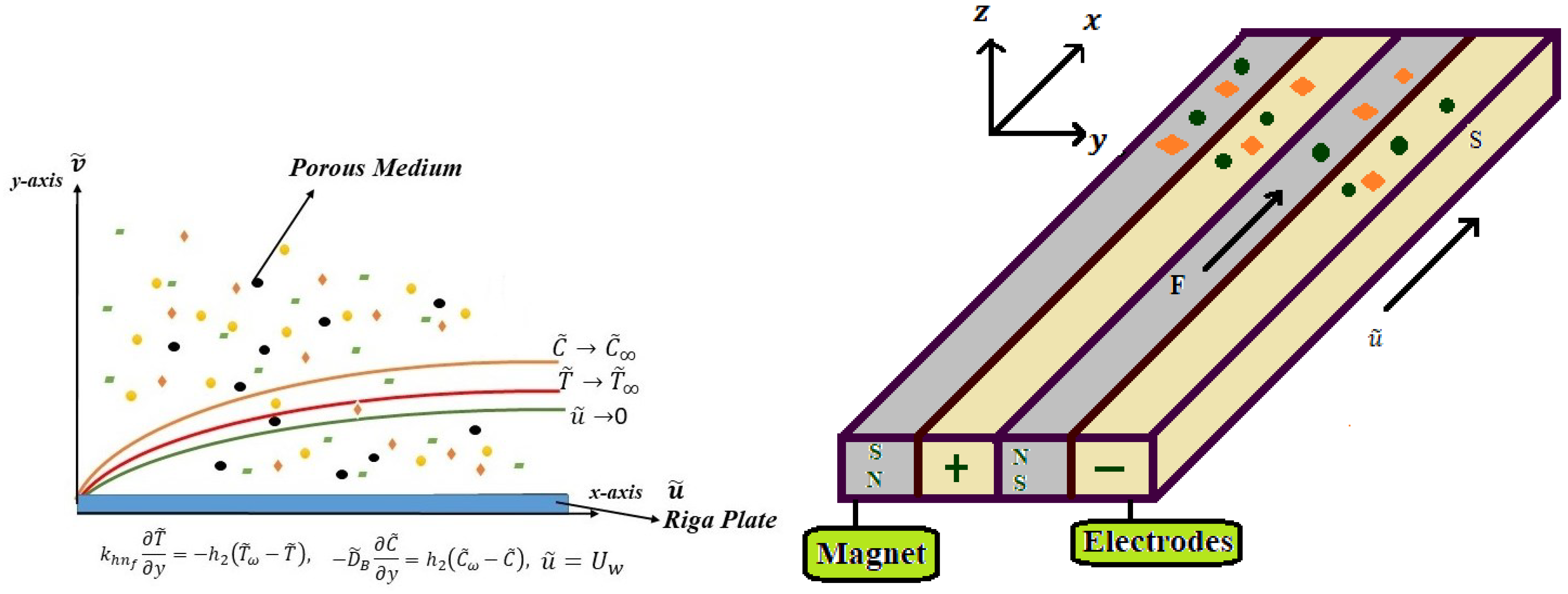
Figure 1. Configuration of this study.
Symmetry 17 01582 g001
Figure 2. Effect of M on f ( η ) : P r = 1.2 , m = 0.3 , N = 0.3 , λ = 0.2 , Q = 0.1 , β = 0.8 , δ = 0.1 ,   F r = 0.5 ,   N b = 0.5 , N t = 0.1 , R d = 0.3 , B i = 0.5 , E c = 0.5 , γ 1 = γ 2 = 0.2 , n = 1 , L e = 1.2 ,   E = 0.2 ,   δ ˜ = 0.1 , σ = 0.3 , α 1 = 0.5 .
Symmetry 17 01582 g002
Figure 3. Effect of β on f ( η ) : P r = 1.2 , m = 0.3 , N = 0.3 , λ = 0.2 , Q = 0.1 , M = 0.2 , δ = 0.1 ,   F r = 0.5 ,   N b = 0.5 , N t = 0.1 , R d = 0.3 , B i = 0.5 , E c = 0.5 , γ 1 = γ 2 = 0.2 , n = 1 , L e = 1.2 ,   E = 0.2 ,   δ ˜ = 0.1 , σ = 0.3 , α 1 = 0.5 .
Symmetry 17 01582 g003
Figure 4. Effect of N on f ( η ) : P r = 1.2 , m = 0.3 , λ = 0.2 , Q = 0.1 , M = 0.2 , β = 0.8 , δ = 0.1 ,   F r = 0.5 ,   N b = 0.5 , N t = 0.1 , R d = 0.3 , B i = 0.5 , E c = 0.5 , γ 1 = γ 2 = 0.2 , n = 1 , L e = 1.2 ,   E = 0.2 ,   δ ˜ = 0.1 , σ = 0.3 , α 1 = 0.5 .
Symmetry 17 01582 g004
Figure 5. Effect of Q on f ( η ) : P r = 1.2 , m = 0.3 , N = 0.3 , λ = 0.2 , M = 0.2 , β = 0.8 , δ = 0.1 ,   F r = 0.5 ,   N b = 0.5 , N t = 0.1 , R d = 0.3 , B i = 0.5 , E c = 0.5 , γ 1 = γ 2 = 0.2 , n = 1 , L e = 1.2 ,   E = 0.2 ,   δ ˜ = 0.1 , σ = 0.3 , α 1 = 0.5 .
Symmetry 17 01582 g005
Figure 6. Effect of δ on f ( η ) : P r = 1.2 , m = 0.3 , N = 0.3 , λ = 0.2 , Q = 0.1 , M = 0.2 , β = 0.8 ,   F r = 0.5 ,   N b = 0.5 , N t = 0.1 , R d = 0.3 , B i = 0.5 , E c = 0.5 , γ 1 = γ 2 = 0.2 , n = 1 , L e = 1.2 ,   E = 0.2 ,   δ ˜ = 0.1 , σ = 0.3 , α 1 = 0.5 .
Symmetry 17 01582 g006
Figure 7. Effect of β on f ( η ) : P r = 1.2 , m = 0.3 , N = 0.3 , λ = 0.2 , Q = 0.1 , M = 0.2 , β = 0.8 ,   δ = 0.1 ,   N b = 0.5 , N t = 0.1 , R d = 0.3 , B i = 0.5 , E c = 0.5 , γ 1 = γ 2 = 0.2 , n = 1 , L e = 1.2 , E = 0.2 , δ ˜ = 0.1 ,   σ = 0.3 ,   α 1 = 0.5 .
Symmetry 17 01582 g007
Figure 8. Effect of λ on f ( η ) : P r = 1.2 , m = 0.3 , N = 0.3 , Q = 0.1 , M = 0.2 , β = 0.8 , δ = 0.1 ,   F r = 0.5 ,   N b = 0.5 , N t = 0.1 , R d = 0.3 , B i = 0.5 , E c = 0.5 , γ 1 = γ 2 = 0.2 , n = 1 , L e = 1.2 ,   E = 0.2 ,   δ ˜ = 0.1 , σ = 0.3 , α 1 = 0.5 .
Symmetry 17 01582 g008
Figure 9. Effect of M on f ( η ) : P r = 1.2 , m = 0.3 , N = 0.3 , λ = 0.2 , Q = 0.1 , β = 0.8 , δ = 0.1 ,   F r = 0.5 ,   N b = 0.5 , N t = 0.1 , R d = 0.3 , B i = 0.5 , E c = 0.5 , γ 1 = γ 2 = 0.2 , n = 1 , L e = 1.2 ,   E = 0.2 ,   δ ˜ = 0.1 , σ = 0.3 , α 1 = 0.5 .
Symmetry 17 01582 g009
Figure 10. Effect of R d on f ( η ) : P r = 1.2 , m = 0.3 , N = 0.3 , λ = 0.2 , Q = 0.1 , M = 0.2 , β = 0.8 ,   δ = 0.1 ,   F r = 0.5 , N b = 0.5 , N t = 0.1 , B i = 0.5 , E c = 0.5 , γ 1 = γ 2 = 0.2 , n = 1 , L e = 1.2 , E = 0.2 ,   δ ˜ = 0.1 ,   σ = 0.3 , α 1 = 0.5 .
Symmetry 17 01582 g010
Figure 11. Effect of B i on f ( η ) : P r = 1.2 , m = 0.3 , N = 0.3 , λ = 0.2 , Q = 0.1 , M = 0.2 , β = 0.8 ,   δ = 0.1 ,   F r = 0.5 , N b = 0.5 , N t = 0.1 , R d = 0.3 , E c = 0.5 , γ 1 = γ 2 = 0.2 , n = 1 , L e = 1.2 , E = 0.2 ,   δ ˜ = 0.1 ,   σ = 0.3 , α 1 = 0.5 .
Symmetry 17 01582 g011
Figure 12. Effect of N b on f ( η ) : P r = 1.2 , m = 0.3 , N = 0.3 , λ = 0.2 , Q = 0.1 , M = 0.2 , β = 0.8 ,   δ = 0.1 ,   F r = 0.5 , N t = 0.1 , R d = 0.3 , B i = 0.5 , E c = 0.5 , γ 1 = γ 2 = 0.2 , n = 1 , L e = 1.2 , E = 0.2 ,   δ ˜ = 0.1 ,   σ = 0.3 , α 1 = 0.5 .
Symmetry 17 01582 g012
Figure 13. Effect of N t on f ( η ) : P r = 1.2 , m = 0.3 , N = 0.3 , λ = 0.2 , Q = 0.1 , M = 0.2 , β = 0.8 ,   δ = 0.1 ,   F r = 0.5 , N b = 0.5 , R d = 0.3 , B i = 0.5 , E c = 0.5 , γ 1 = γ 2 = 0.2 , n = 1 , L e = 1.2 , E = 0.2 ,   δ ˜ = 0.1 ,   σ = 0.3 , α 1 = 0.5 .
Symmetry 17 01582 g013
Figure 14. Effect of M on f ( η ) : P r = 1.2 , m = 0.3 , N = 0.3 , λ = 0.2 , Q = 0.1 , β = 0.8 , δ = 0.1 ,   F r = 0.5 ,   N b = 0.5 , N t = 0.1 , R d = 0.3 , B i = 0.5 , E c = 0.5 , γ 1 = γ 2 = 0.2 , n = 1 , L e = 1.2 ,   E = 0.2 ,   δ ˜ = 0.1 , σ = 0.3 , α 1 = 0.5 .
Symmetry 17 01582 g014
Figure 15. Effect of E on f ( η ) : P r = 1.2 , m = 0.3 , N = 0.3 , λ = 0.2 , Q = 0.1 , M = 0.2 , β = 0.8 ,   δ = 0.1 ,   F r = 0.5 ,   N b = 0.5 , N t = 0.1 , R d = 0.3 , B i = 0.5 , E c = 0.5 , γ 1 = γ 2 = 0.2 , n = 1 , L e = 1.2 ,   δ ˜ = 0.1 ,   σ = 0.3 , α 1 = 0.5 .
Symmetry 17 01582 g015
Figure 16. Effect of N b on f ( η ) : P r = 1.2 , m = 0.3 , N = 0.3 , λ = 0.2 , Q = 0.1 , M = 0.2 , β = 0.8 ,   δ = 0.1 ,   F r = 0.5 , N t = 0.1 , R d = 0.3 , B i = 0.5 , E c = 0.5 , γ 1 = γ 2 = 0.2 , n = 1 , L e = 1.2 , E = 0.2 ,   δ ˜ = 0.1 ,   σ = 0.3 , α 1 = 0.5 .
Symmetry 17 01582 g016
Figure 17. “Effect of N t on f ( η ) : P r = 1.2 , m = 0.3 , N = 0.3 , λ = 0.2 , Q = 0.1 , M = 0.2 , β = 0.8 ,   δ = 0.1 ,   F r = 0.5 , N b = 0.5 , R d = 0.3 , B i = 0.5 , E c = 0.5 , γ 1 = γ 2 = 0.2 , n = 1 , L e = 1.2 , E = 0.2 ,   δ ˜ = 0.1 ,   σ = 0.3 , α 1 = 0.5 ”.
Symmetry 17 01582 g017
Figure 18. Effect of σ on f ( η ) : P r = 1.2 , m = 0.3 , N = 0.3 , λ = 0.2 , Q = 0.1 , M = 0.2 , β = 0.8 ,   δ = 0.1 ,   F r = 0.5 , N b = 0.5 , N t = 0.1 , R d = 0.3 , B i = 0.5 , E c = 0.5 , γ 1 = γ 2 = 0.2 , n = 1 , L e = 1.2 ,   E = 0.2 ,   δ ˜ = 0.1 , α 1 = 0.5 .
Symmetry 17 01582 g018
Figure 19. Effect of α 1 on f ( η ) : P r = 1.2 , m = 0.3 , N = 0.3 , λ = 0.2 , Q = 0.1 , M = 0.2 , β = 0.8 ,   δ = 0.1 ,   F r = 0.5 , N b = 0.5 , N t = 0.1 , R d = 0.3 , B i = 0.5 , E c = 0.5 , γ 1 = γ 2 = 0.2 , n = 1 , L e = 1.2 ,   E = 0.2 ,   δ ˜ = 0.1 , σ = 0.3 .
Symmetry 17 01582 g019
Figure 20. ANN training for Powell–Eyring parameter. (a) Mean squared error. (b) Training states. (c) Error histogram. (d) Regression analysis. (e) Function fit.
Symmetry 17 01582 g020
Figure 21. ANN training for thermal radiation parameter. (a) Mean squared error. (b) Training states. (c) Error histogram. (d) Regression analysis. (e) Function fit.
Symmetry 17 01582 g021
Figure 22. ANN training for thermophoresis parameter. (a) Mean squared error. (b) Training states. (c) Error histogram. (d) Regression analysis. (e) Function fit.
Symmetry 17 01582 g022
Figure 23. Comparison of ANN and BVP4C for different parameters. (a) Velocity for N. (b) Temperature for R d . (c) Concentration for N t .
Symmetry 17 01582 g023
Table 1. Skin friction coefficient numerical results vs. multiple parameter values.
MNQ σ Fr Re 0.5 C f
0.20.30.10.10.5−0.7402
0.4 −0.6274
0.6 −0.4701
0.10.2 −0.6452
0.5 −1.0000
0.8 −1.2643
0.30.3 −0.7775
0.6 −1.0956
0.9 −1.3397
0.10.2 −0.7548
0.4 −0.6926
0.6 −0.6101
0.10.4−0.7888
0.8−0.7283
1.2−0.6307
Table 2. Nusselt number numerical results vs. various parameter values.
M Rd Nb Nt Bi Re 0.5 Nu
0.20.30.50.10.50.2841
0.4 0.2591
0.6 0.2368
0.10.4 0.3199
0.7 0.3819
1.0 0.4390
0.30.6 0.2956
0.8 0.2909
1.0 0.2861
0.50.3 0.2932
0.5 0.2884
0.7 0.2836
0.10.40.2621
0.70.3532
1.00.4099
Table 3. ANN-LMA training summary.
Epoch MSE Gradient mu
208 8.5193 × 10 10 9.9474 × 10 8 1 × 10 9 Powell–Eyring
273 7.9108 × 10 9 9.9139 × 10 8 1 × 10 9 Rd
221 1.5925 × 10 8 9.9156 × 10 8 1 × 10 8 Nt
Disclaimer/Publisher’s Note: The statements, opinions and data contained in all publications are solely those of the individual author(s) and contributor(s) and not of MDPI and/or the editor(s). MDPI and/or the editor(s) disclaim responsibility for any injury to people or property resulting from any ideas, methods, instructions or products referred to in the content.