Positioning-Based Uplink Synchronization Method for NB-IoT in LEO Satellite Networks

Abstract

With the growth of Internet of Things (IoT) business demands, NB-IoT integrating low earth orbit (LEO) satellite communication systems is considered a crucial component for achieving global coverage of IoT networks in the future. However, the long propagation delay and significant Doppler frequency shift of the satellite-to-ground link pose substantial challenges to the uplink and downlink synchronization in LEO satellite-based NB-IoT networks. To address this challenge, we first propose a Multiple Segment Auto-correlation (MSA) algorithm to detect the downlink Narrow-band Primary Synchronization Signal (NPSS), specifically tailored for the large Doppler frequency shift of LEO satellites. After detection, downlink synchronization can be realized by determining the arrival time and frequency of the NPSS. Then, to complete the uplink synchronization, we propose a position-based scheme to obtain the Timing Advance (TA) values and pre-compensated Doppler shift value. In this scheme, we formulate a time difference of arrival (TDOA) equation using the arrival times of NPSSs from different satellites or at different times as observations. After solving the TDOA equation using the Chan method, the uplink synchronization is completed by obtaining the TA values and pre-compensated Doppler shift value from the terminal position combined with satellite ephemeris. Finally, the feasibility of the proposed scheme is verified in an Iridium satellite constellation. Compared to conventional GNSS-assisted methods, the approach proposed in this paper reduces terminal power consumption by 15–40%. Moreover, it achieves an uplink synchronization success rate of over 98% under negative SNR conditions.

1. Introduction

As the core direction of the development of next-generation information technologies, the Internet of Everything (IoE) is a key enabler for future digitalization and intelligent transformation. To realize the vision of IoE in future 6G networks, achieving global network coverage is a fundamental prerequisite. However, the construction and maintenance costs of terrestrial base stations in remote areas are prohibitively high. Currently, more than 80% of land areas and over 95% of oceans are not covered by terrestrial networks. As a result, the use of satellites for global coverage of wireless networks has become a research hotspot [1,2].

For terminals in these regions that require Positioning, Navigation, and Timing (PNT) services, Global Navigation Satellite System (GNSS) technologies are commonly used to obtain location and related information [3]. Nevertheless, GNSS suffers from several drawbacks, including high power consumption, frequent signal unavailability, and reliance on external systems. As an alternative to GNSS, PNT services via low earth orbit (LEO) satellites are gaining increasing attention [4,5]. Compared to medium earth orbit GNSS satellites, LEO satellites are much closer to the earth, allowing for stronger satellite signals that can provide PNT services even under GNSS-denied conditions—such as signal blockage, inability to receive signals from four GNSS satellites simultaneously, or signal interference. Although LEO satellite-based positioning has lower accuracy than GNSS, it is more valuable for IoT terminals with low power consumption requirements and less stringent positioning accuracy needs [6,7].

NB-IoT is a mature, widely deployed low-power wide-area (LPWA) technology in terrestrial networks. It is one of the communication technologies designed for the Internet of Things, targeting application scenarios characterized by low data rates, low power consumption, and massive device connectivity. Similar technologies include LoRa. Earlier this year, Iridium Communications (McLean, VA, USA), a well-established satellite operator, officially launched Project Stardust, a direct-to-satellite NB-IoT Non-Terrestrial Network (NTN) initiative based on 3GPP standards. The project has begun to foster collaboration across the NB-IoT industry ecosystem.

One of the major challenges in LEO satellite-to-ground networks is uplink synchronization. Terrestrial networks use Timing Advance (TA) mechanisms to achieve uplink synchronization [8]. Traditional Timing Advance strategies require user equipment to first capture downlink synchronization signals and extract synchronization information. However, in satellite networks, the vast distance between satellites and ground terminals exceeds the maximum allowable TA value. Furthermore, the high-speed movement of satellites causes rapid TA value obsolescence, necessitating frequent updates. Traditional methods in which terminals transmit preamble signals to obtain TA values are not feasible in satellite channels [9]. To address this, 3GPP has proposed that terminals may use GNSS to obtain their positions and then calculate TA values using satellite ephemeris data for synchronization [10,11]. While this approach is viable for 5G NR terminals, it is unsuitable for NB-IoT devices due to GNSS’s high power consumption [12,13]. Therefore, it is essential to develop a novel uplink synchronization solution tailored to IoT devices with low-power requirements.

1.1. Related Work

In the context of achieving uplink synchronization for terminals without GNSS assistance in LEO satellite scenarios, several studies have been conducted. Paper [14] compares GNSS and LEO-based positioning schemes and proposes evaluation metrics for IoT terminals to perform PNT services, including positioning accuracy, power consumption, hardware availability, and network accessibility. These metrics will also serve as key indicators for evaluating the proposed scheme in this paper. Paper [15] suggests that terminals can obtain TDOA and FDOA measurements over a time window of 2–12 s to estimate their positions and subsequently calculate TA values using satellite ephemeris broadcast data. However, this method requires the terminal to remain in receive mode for extended periods, resulting in significant power consumption, making it unsuitable for low-power NB-IoT devices. Moreover, the paper does not provide a detailed analysis of power consumption. In [16], a method called SPIN is proposed, in which the terminal measures the downlink primary synchronization signal to acquire observation data and then solves an observation equation. The paper also includes a comparison of power consumption with GNSS-based approaches. However, it does not analyze the specific signal format nor describe how the observations are obtained. In [17], a receiver model is designed that incorporates pilot signal insertion and Doppler shift estimation. While it provides a complete receiver framework, it requires modification of the existing signal structure and leads to increased power consumption on the transmitter side. Paper [18] proposes that, for NB-IoT terminals, uplink frequency synchronization can be achieved by compensating the downlink frequency offset estimation into the uplink and performing frequency tracking. However, this study does not detail a specific downlink synchronization mechanism. Additionally, some approaches estimate uplink TA values without relying on terminal position by modifying the signal structure. Papers [19,20] propose 5G synchronization signal detection algorithms under LEO satellite channels that utilize the multipath energy window of the signal and cyclic prefix-based joint time-frequency estimation method. These methods aim to address the severe Doppler shift inherent in LEO channels, which renders traditional synchronization techniques ineffective. Therefore, it is necessary to redesign detection algorithms specifically for synchronization signals to improve the overall synchronization performance of the system.

1.2. Contributions

In this paper, we investigate the uplink synchronization issue of NB-IoT in LEO satellite scenarios. The terminal obtains observation values by detecting the NPSS, formulates a TDOA equation to determine its position, and then estimates the TA and Doppler offset using satellite ephemeris. The main contributions of this work are summarized as follows:

(1)

Position-aided uplink synchronization for NB-IoT terminals: To address the challenges of large Doppler shifts and varying numbers of visible satellites in LEO satellite scenarios, we propose a position-aided uplink synchronization method. Observation values are obtained through NPSS detection, and a TDOA equation is constructed to estimate the terminal’s position, which is then combined with satellite ephemeris to complete uplink synchronization.

(2)

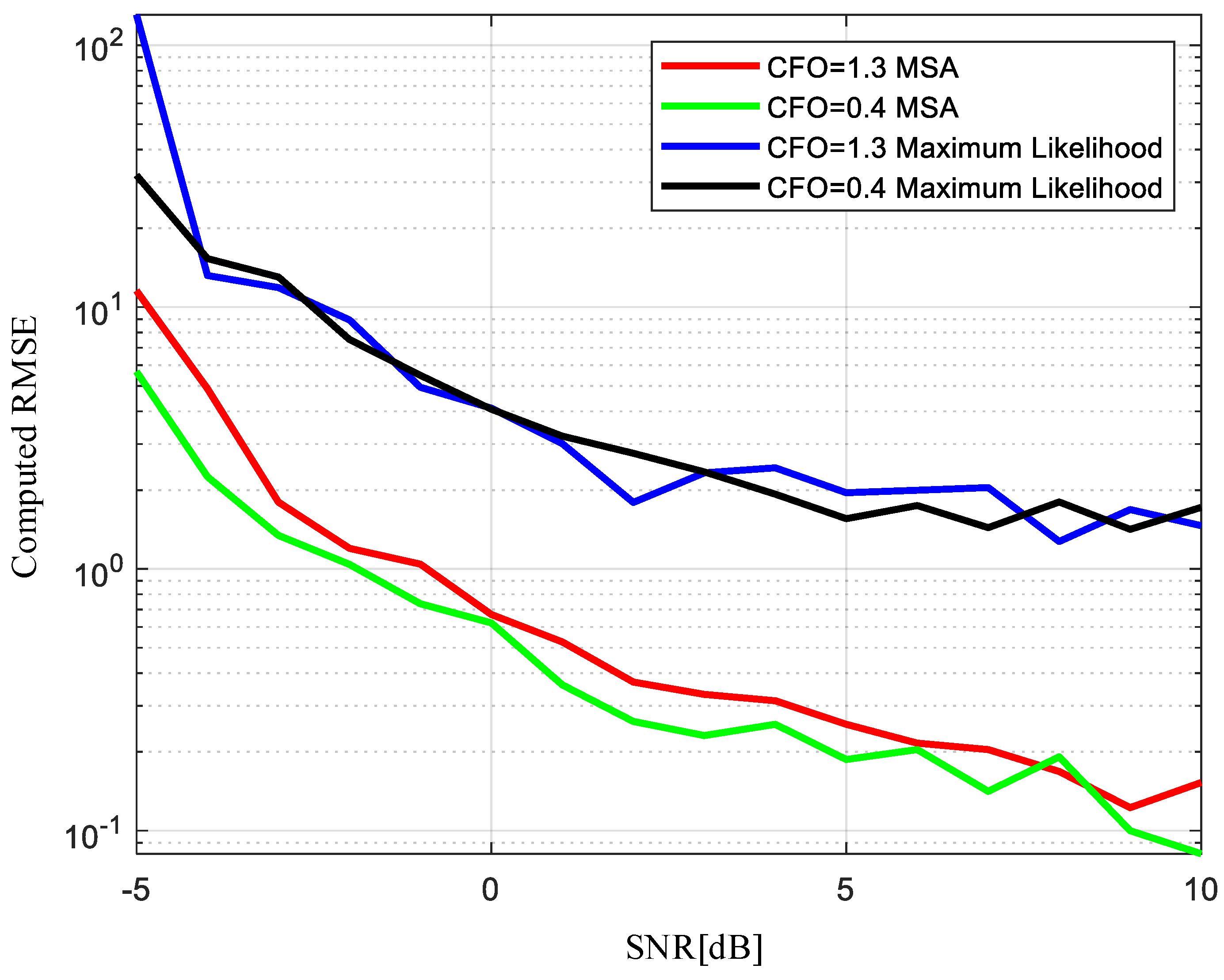
Multiple Segment Auto-correlation (MSA) detection method for NPSS: To cope with the detection of NPSSs under the high-dynamics and large Doppler shift conditions of LEO satellites, we propose the MSA algorithm, which exploits the symmetry of NPSSs. This algorithm leverages the time-domain repetition property of the NPSS to achieve robust acquisition of timing and frequency observation values under severe Doppler conditions.

(3)

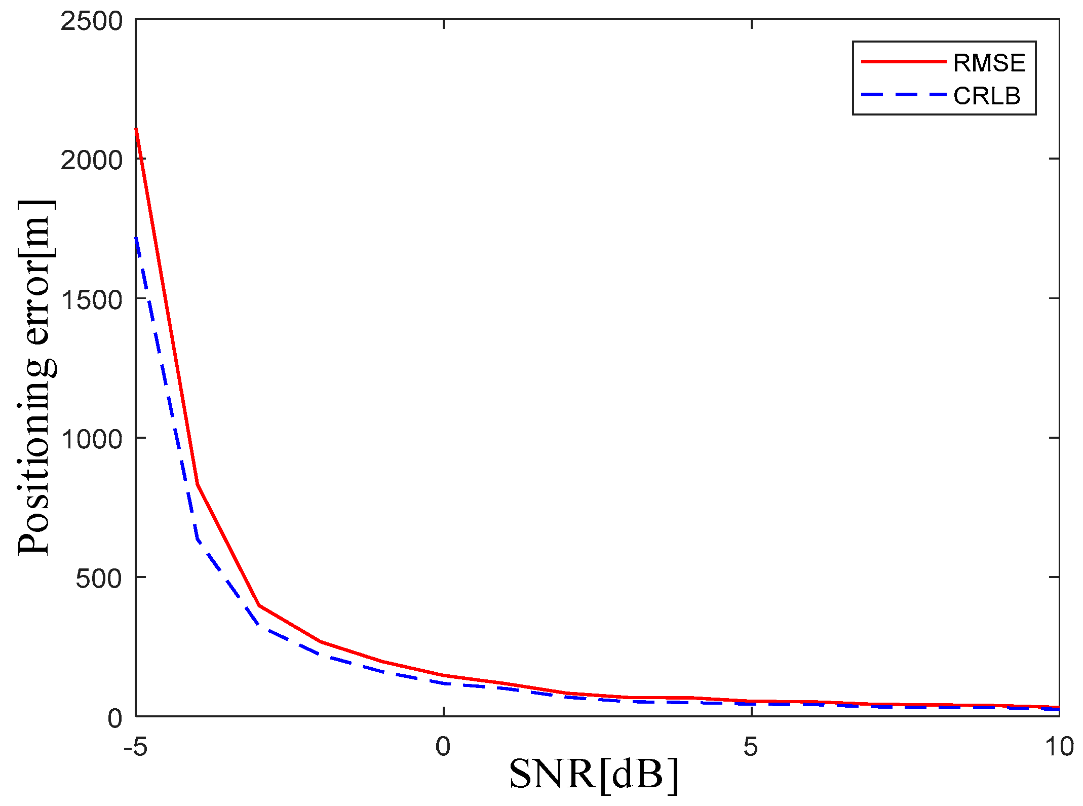
Terminal positioning via NPSS-based delay observations: Based on the time delay observations from NPSSs, we establish TDOA equations under different numbers of visible satellites to estimate the terminal position. Furthermore, we derive the Cramér–Rao lower bound (CRLB) and analyze the power consumption characteristics of IoT terminals. Under an SNR ratio of −2 dB, the positioning error can be maintained at around 200 m.

(4)

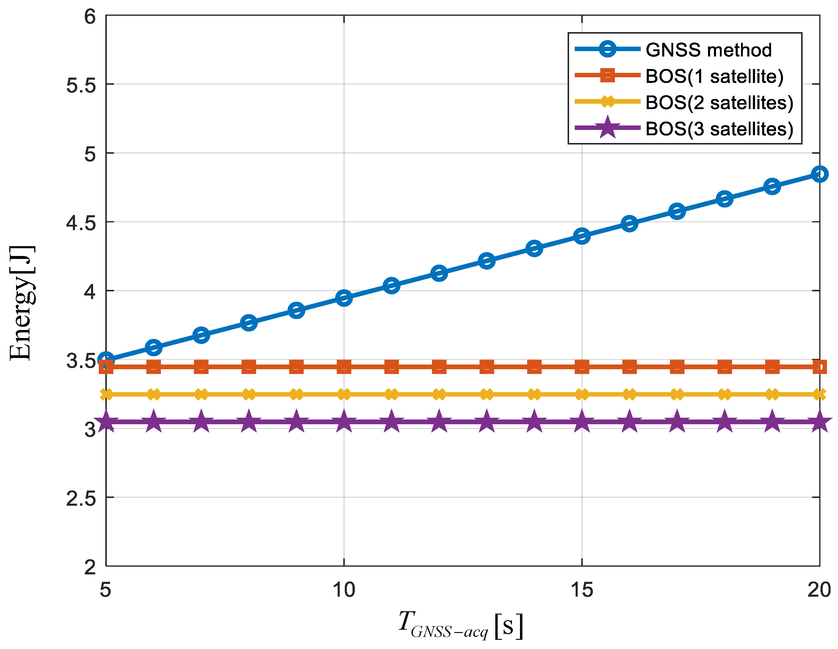
Simulation under the Iridium constellation: We simulate the performance of the proposed algorithm under the Iridium satellite constellation configuration. The simulation results demonstrate that the approach proposed in this paper reduces terminal power consumption by 15–40% while still meeting the uplink synchronization requirements of the NB-IoT system.

2. System Model

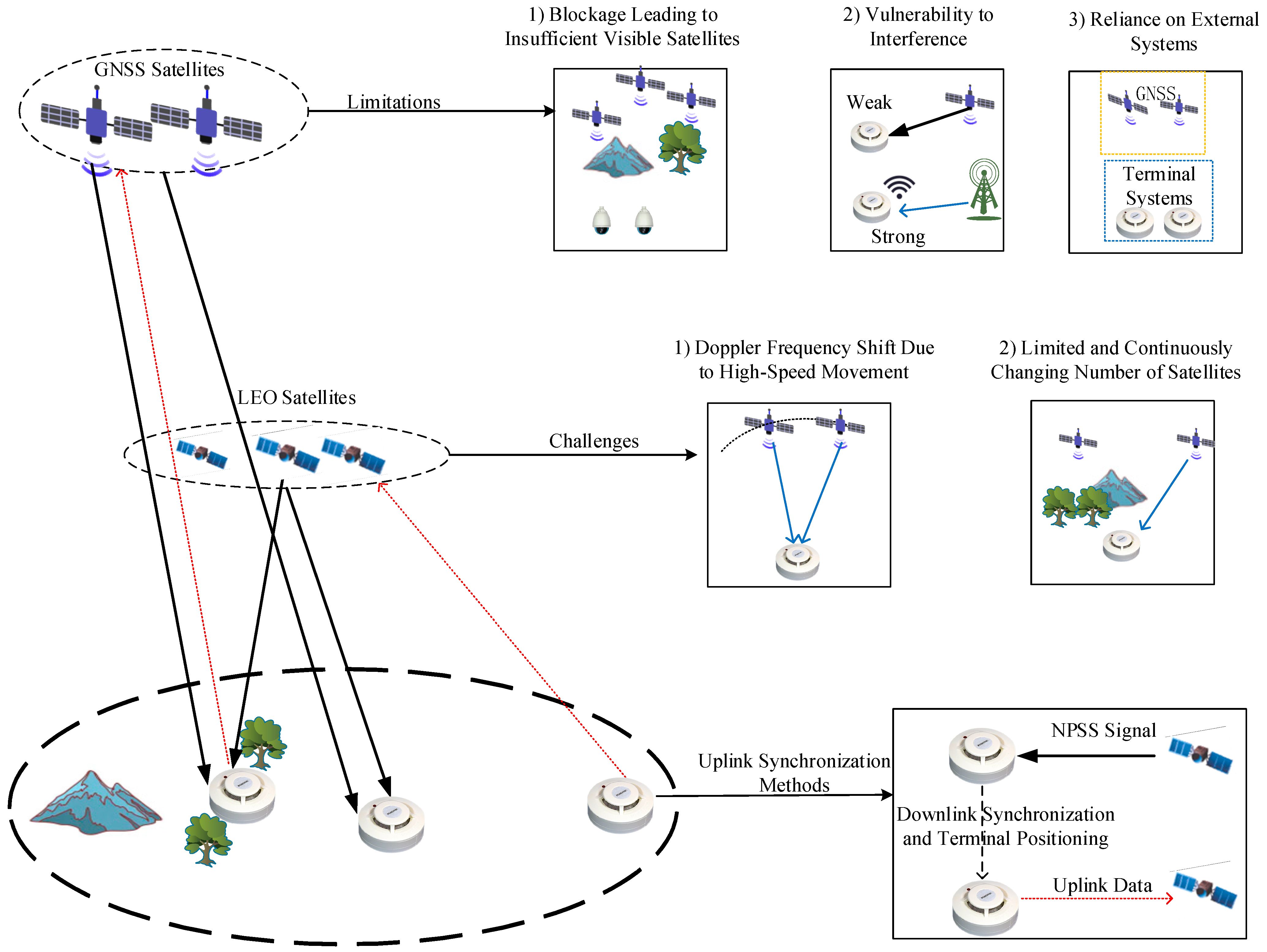
2.1. Problem Scenario and Technical Challenges

Figure 1 illustrates the system architecture of an LEO and GNSS satellite-based IoT network built upon the NB-IoT framework. The NB-IoT system adopts an Orthogonal Frequency Division Multiplexing (OFDM) transmission scheme. During uplink synchronization, the base station (BS) requires that the uplink signals from all user equipment (UE) arrive nearly simultaneously, ideally within one CP duration, to ensure correct demodulation. To achieve this, NB-IoT employs a TA mechanism: terminals located farther from the BS are instructed to transmit earlier, so that their signals arrive at the BS in alignment with others. In terrestrial NB-IoT systems, the terminal first performs time and frequency synchronization by detecting the downlink synchronization signal broadcast by the BS. It cross-correlates the received signal with a local reference to identify the peak position, enabling synchronization. This is followed by a random access procedure, where the terminal sends a preamble sequence to the BS. Upon receiving the Message 1 (MES1), the BS detects the preamble, calculates the required TA value, and sends it back to the UE via Message 2 (MES2).

However, this conventional TA-based synchronization strategy is not directly applicable in satellite NB-IoT systems. First, the large Doppler frequency shift in satellite channels causes traditional correlation-based synchronization algorithms to fail. Second, the high mobility of satellites results in a very short validity period for the TA value, necessitating frequent updates and thus consuming excessive signaling resources.

To address this, 3GPP proposes that most NTN terminals be equipped with GNSS receivers for uplink synchronization. With knowledge of its own position and satellite ephemeris data broadcast by the satellite, a terminal can compute the required TA value and the pre-compensated Doppler shift. However, in practical NB-IoT LEO satellite communication scenarios, GNSS signal reception may be blocked due to environmental obstructions, or the terminal may be unable to simultaneously receive signals from four GNSS satellites. Additionally, GNSS signals may suffer from interference. For NB-IoT devices that are power-constrained, relying on a GNSS that is external to the system results in substantial additional power consumption. This has motivated research into leveraging the communication signals themselves for PNT services. In this approach, the communication system provides terminal positioning capabilities without GNSS assistance. However, realizing positioning using communication signals in LEO satellite systems faces significant technical challenges, including large Doppler shifts and time-varying numbers of visible satellites.

To this end, this paper explores the use of the NB-IoT downlink broadcast signal, namely the Narrowband Primary Synchronization Signal, to enable terminal positioning. By combining this with satellite ephemeris data, a pre-compensation-based uplink synchronization scheme is proposed, specifically tailored to LEO satellite scenarios.

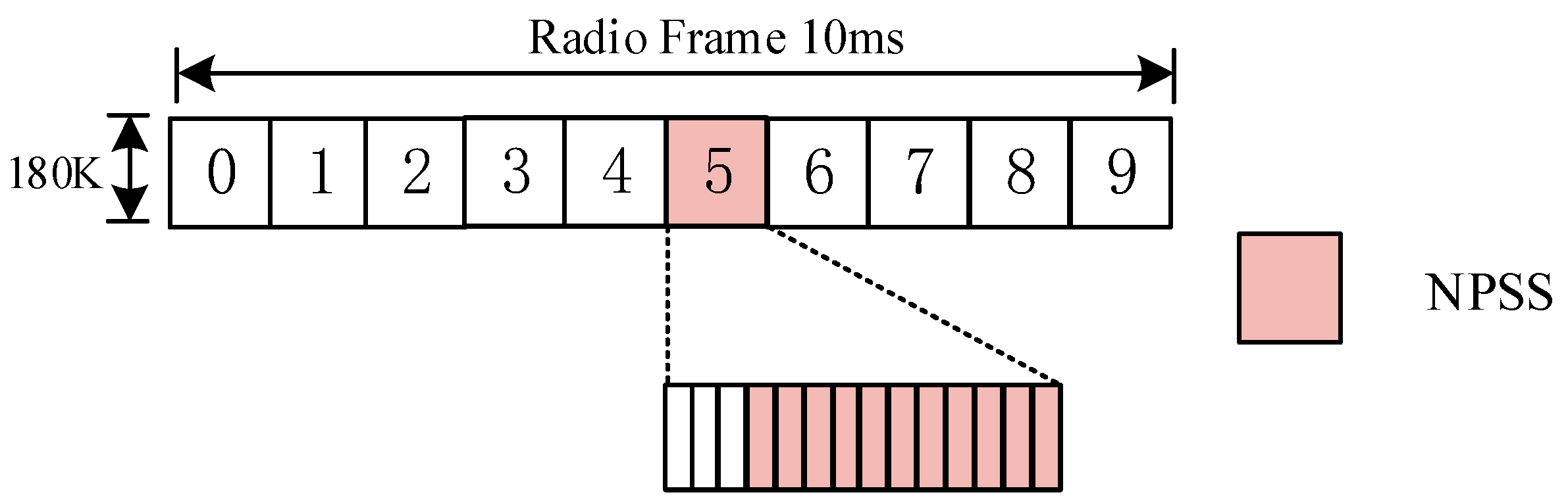
2.2. Downlink NPSS in NB-IoT

This study focuses on utilizing the NPSS received by NB-IoT terminals to estimate time-delay and Doppler shift observations. Figure 2 illustrates the structure of the downlink NPSS in NB-IoT systems. In NB-IoT, each radio frame (RF) has a duration of 10 ms and is composed of 10 subframes (SFs), each lasting 1 ms. Each subframe consists of two 0.5 ms slots, and each slot contains seven OFDM symbols. The NPSS is transmitted in the fifth subframe of every radio frame, with a repetition period of 10 ms.

The NPSS in the NB-IoT downlink is generated based on an 11-length short Zadoff–Chu (ZC) sequence using the following formula:

$$S(k)=e^{-{\displaystyle \frac{j\pi uk(k-1)}{11}}},k=1,2,\dots ,11$$

(1)

Here, $k$ denotes the sequence index, and $u$ is the physical root index used to generate the ZC sequence. In the NB-IoT system, $u=5$. The resulting 11-point short ZC sequence is transformed into the time domain using the inverse fast Fourier transform (IFFT). By adding a CP and repeating the signal 10 times according to the rules, we obtain the NPSS $x(n)$. The corresponding signal received by the NB-IoT terminal, denoted as $y(n)$, is expressed as [15]:

$$y(n)={\displaystyle \sum _{l=0}^{L-1}h(l)x(n-\delta -l)e^{j2\pi n\epsilon /N}}+\omega (n)$$

(2)

where $\delta$ represents the normalized symbol timing offset, $\epsilon$ represents the normalized carrier frequency offset, $n$ denotes the sample index, $N$ denotes the point of FFT, $h(l)$ represents the impulse response of the multipath channel with $L$ uncorrelated taps, and $w(n)$ is additive white Gaussian noise (AWGN) with zero mean and variance ${\sigma }^2$.

The NPSS is generated from an 11-point short ZC sequence. The ZC sequence has excellent correlation properties, as its autocorrelation function is nearly zero at all non-zero lags. However, in satellite channels with large Doppler shifts, the peak of the correlation function is significantly degraded, which affects synchronization accuracy.

Compared with the 5G primary synchronization signal (PSS), which occupies 127 subcarriers in the frequency domain and spans 1 OFDM symbol in the time domain, the NB-IoT NPSS only occupies 11 subcarriers in the frequency domain but spans 11 OFDM symbols in the time domain. This design aligns with NB-IoT’s narrowband characteristics—the system has a bandwidth of only 180 kHz, necessitating a longer time-domain signal duration to ensure sufficient detection performance. Therefore, the synchronization method proposed in Section 3 is specifically designed to exploit the time-domain symmetry of NPSS under large Doppler conditions.

3. Position-Aided Uplink Synchronization Method

To address the uplink synchronization issue of NB-IoT terminals in LEO satellite networks, this paper proposes a position-aided uplink synchronization method named based on synchronization signals (BOS). The method first detects the NPSS transmitted by the satellite to estimate time delay and Doppler shift observation values. Then, a TDOA equation is constructed using the delay observations and satellite ephemeris to solve for the terminal’ s position. Finally, the TA value and Doppler pre-compensation are calculated based on the terminal position and satellite ephemeris, completing uplink synchronization.

Furthermore, to assess the theoretical performance bound of the proposed algorithm, the CRLB for the positioning algorithm is derived. Based on this, a receiver block diagram is designed for the terminal, and the power consumption of the uplink synchronization process is analyzed under different numbers of visible satellites.

3.1. NPSS Detection

To tackle the significant Doppler shift in satellite channels, this paper proposes a time delay estimation method for NPSS named Multi-Section Correlation Algorithm (MSA), which combines coarse and fine estimation stages. Building upon this, a hybrid time-frequency domain approach is used to estimate the Doppler shift observation value, improving the accuracy of time delay and Doppler estimation under high-dynamic LEO satellite channels. The overall estimation process, shown in Figure 3, includes three main parts: coarse estimation of time delay, fine estimation of time delay, and Doppler shift observation estimation. First, for each sampling point, coarse synchronization detection is performed on a signal with a length of one NPSS by dividing it into 11 equal segments and applying segment-wise autocorrelation to obtain a coarse synchronization point. Next, a more accurate calculation is carried out in the frequency domain around the coarse synchronization point by correlating the signal with 11 locally stored ZC sequences, yielding the fine synchronization point. Finally, Doppler frequency offset estimation and compensation are performed on the time-synchronized signal.

3.1.1. Coarse Estimation of Time Delay Observations

Due to the time-domain repetition characteristics of the NPSS, the traditional autocorrelation-based Doppler cancellation algorithm produces significant side peaks at positions corresponding to one OFDM symbol interval, which adversely affect detection performance. Therefore, when using conjugate multiplication of the signal to mitigate Doppler frequency offset, it is necessary to fully exploit the time-domain autocorrelation properties of the ZC sequence to design an appropriate metric function. We adopt the commonly used 1.92 MHz sampling rate for NB-IoT, which, combined with the 15 kHz subcarrier spacing, results in an FFT size of 128. The specific steps of the algorithm are described below.

$y(n)$ is the received signal defined in Equation (2). For each sampling point $n$, the subsequent signal segment of one NPSS duration is divided equally into 11 parts, yielding $z_1,z_2,z_3\dots \dots z_{11}$:

$$z_m=y\left\{\left[n+N\cdot \left(m-1\right)\right]:\left[n+N\cdot m\right]\right\},m=1,2,\dots \dots ,11;$$

(3)

As shown in Figure 4, each of the 11 signal segments is cross-correlated with the complex conjugates of the other 10 segments, resulting in 11 correlation values $v_m$:

$$\begin{array}{ll}{v}_m& ={\displaystyle \sum _{i=1}^{11}{z}_m\cdot {z^{*}}_i}\\ & ={\displaystyle \sum _{i=1}^{11}{\displaystyle \sum _{d=0}^{N-1}y(n+d+N\cdot m-N)\cdot y{(n+d+N\cdot i)}^{*}}}, i\ne m\end{array}$$

(4)

Here, $d$ is a counting variable introduced by the correlation operation. $i\ne m$ holds because the autocorrelation values of the individual segments are large. To prevent these from contributing to the final result and causing false peaks, they are excluded from the calculation. All frames are independent of each other and free from corruption. We ignore multipath and other interference. Substituting Equation (2) into the computation yields:

$$v_m={\displaystyle \sum _{i=1}^{11}{\displaystyle \sum _{d=0}^{N-1}x(n+d+N*m-N-\delta )\cdot x(n+d+N*i-\delta )}}\cdot e^{j2\pi (n+d+N*m-N)\epsilon /N}\cdot e^{-j2\pi (n+d+N*l)\epsilon /N}$$

(5)

For each sampling point $n$, 11 different correlation values $v_m$ are obtained corresponding to different values of $m$. The metric value $p(n)$ at sampling point $n$ is defined as the minimum among these 11 correlation values:

$$p(n)={\left[\min \left(v_1,v_2,\dots ,v_{11}\right)\right]}^2$$

(6)

According to the position of the sampling point $n$, the sampling point distribution is classified into three categories in Figure 5: partially overlapping, fully aligned, and the start positions of adjacent symbols. Correlation between two identical ZC sequences produces a distinct peak, but in the presence of Doppler frequency offset, the peak may be reduced or shifted.

(I)

$n\ne \delta +a\cdot N,a=0,\pm 1,\pm 2\dots \dots ;$ When the current sampling point is located in the middle of an OFDM symbol or outside the NPSS, the result is small due to the correlation properties of the ZC sequence.

(II)

$n=\delta$; When the current sampling point corresponds to the start position of the NPSS, a peak appears. Due to the time-domain repetition property of NPSS, the 11 OFDM symbols starting from the beginning are identical. Our algorithm fully exploits this characteristic, so we can get $x(d+N\ast m-N)=x(d+N\cdot i)=x(d)$. The resulting metric $v(m)$ is calculated as follows:

$$\begin{array}{ll}v(m)& ={\displaystyle \sum _{i=1}^{11}{e}^{j2\pi \epsilon (m-i-1)}{\displaystyle \sum _{d=0}^{N-1}x(d+N*m-N)\cdot x(d+N\cdot i)}}\\ & ={\displaystyle \sum _{i=1}^{11}{e}^{j2\pi \epsilon (m-i-1)}{\displaystyle \sum _{d=0}^{N-1}{\left|x(d)\right|}^2}}\\ & =A{\displaystyle \sum _{i=1}^{11}{e}^{j2\pi \epsilon (m-i-1)}}\end{array}$$

(7)

In the final result, $A={\displaystyle \sum _{d=0}^{N-1}{\left|x(d)\right|}^2}$ is a fixed constant, and ${\displaystyle \sum _{i=1}^{11}{e}^{j2\pi \epsilon (m-i-1)}}$ is unaffected by carrier frequency offset $\epsilon$. Therefore, the resulting peak is not influenced by Doppler shift. At this point, the values $v(m)$ corresponding to different $m$ are similar, and the minimum among them is taken as the metric value at sampling point $n$.

(III)

$n=\delta +a\cdot N,a=\pm 1,\pm 2\dots \dots \pm 11;$ When the current sampling point is located at an integer multiple of the OFDM symbol interval adjacent to the actual synchronization point, a peak may also appear. However, the resulting values of $v(m)$ vary significantly across different $m$ values. The minimum $v(m)$ is approximately equivalent to the correlation value with uncorrelated noise $x(n)$, resulting in a small metric value at sampling point $n$.

By examining the detection metric over all sampling points $n$, the location of the peak indicates the coarse synchronization point ${\widehat{n}}_k$:

$${\widehat{n}}_k=\underset{n}{\max }p(n)$$

(8)

3.1.2. Fine Estimation of Time Delay Observations

In NB-IoT LEO satellite communication scenarios, situations such as low satellite elevation angles or signal blockage often result in low SNR at the terminal. To enhance synchronization performance under low SNR conditions, a more accurate synchronization algorithm is applied in the frequency domain based on the coarse estimation. Performing more intensive computations around the coarse synchronization point can improve estimation accuracy under low SNR conditions. Specifically, the sampling point obtained from the coarse estimation algorithm is used as the coarse synchronization point. Then, leveraging the good frequency-domain correlation properties of the ZC sequence, precise synchronization is performed in the frequency domain.

First, a segment of 40 samples before and after the coarse synchronization point ${\widehat{n}}_k$ is selected and transformed into the frequency domain using an FFT of length $N$ to obtain $r(k)$:

$$r(k)=FFT\left[y\left(n\right)\right]$$

(9)

$r(k)$ denotes the FFT result of the received signal when processing begins from some sampling point before timing synchronization is achieved.

$s(k)$ is the locally generated 11-element ZC sequence; its generation formula is given in Equation (1). By performing circular shifts on $s(k)$, 11 local reference sequences $z{c}_1,z{c}_2,\dots \dots z{c}_{11}$ are obtained. $k$ is a counting variable. Each of these reference sequences is then correlated with the FFT-processed received signal to identify the peak and determine the fine timing point, resulting in 11 correlation values:

$$u_{i,n}={\displaystyle \sum _{k=1}^{11}r(k)\cdot z{c}_i(k)},i=1,2,\dots ,11$$

(10)

The maximum value of $u_{i,n}$ is selected as the metric value for the corresponding sampling point. By performing correlation in the frequency domain with the circularly shifted local sequences and selecting the maximum value, the influence of Doppler frequency offset is mitigated. This process is repeated for the sampling points near the coarse synchronization point, and the metric values of each sampling point are plotted. The point corresponding to the maximum value is designated as the fine synchronization point $\widehat{n}$:

$$\widehat{n}=\underset{n}{\max }(u_{1,n}, u_{2,n}\dots u_{11,n})$$

(11)

This fine synchronization algorithm effectively enhances detection accuracy in low signal-to-noise ratio environments, thereby improving the overall uplink synchronization performance of the terminal.

3.1.3. Frequency Offset Estimation Algorithm

After completing time synchronization, frequency synchronization needs to be performed to complete the entire downlink synchronization process. Given the known starting position of the NPSS, we begin by performing an FFT on the signal starting from the fine synchronization point, using a length equivalent to one OFDM symbol, to convert it into the frequency domain:

$$y(k)=FFT\left[y\left(n\right)\right]$$

(12)

where $y(k)$ represents the FFT output based on the correctly aligned sampling point after timing synchronization has been completed. $y(k)$ is correlated in parallel with the 11 local sequences $z{c}_1,z{c}_2,\dots \dots z{c}_{11}$ to estimate the integer multiple frequency offset. ${\epsilon }_i$ is the integer part of the Doppler frequency offset, and ${\epsilon }_f$ is the fractional part. In the algorithm, these two components are calculated separately. The local sequence that produces the maximum correlation value is identified, and the corresponding integer frequency offset ${\epsilon }_i$ is eliminated. This results in the integer frequency offset compensation factor $b$:

$$b=e^{-j2\pi {\epsilon }_{i}n/N}$$

(13)

After multiplying $b$ with the received signal, the remaining signal with only the fractional frequency offset ${\epsilon }_i$ is expressed as:

$$\begin{array}{ll}{y}_i(n)& =x(n)e^{j2\pi n\epsilon /N}\cdot e^{-j2\pi {\epsilon }_i\cdot n/N}\\ & =x(n)e^{j2\pi n{\epsilon }_f/N}\end{array}$$

(14)

The fractional frequency offset ${\widehat{\epsilon }}_f$ is estimated by performing correlation calculations in the time domain:

$$\begin{array}{ll}\chi & ={\displaystyle \sum _{n=0}^{N-1}{y}_i\left(n\right)\cdot y_i\left(n+N\right)}\\ & ={\displaystyle \sum _{n=0}^{N-1}x(n)e^{j2\pi n{\epsilon }_i/N}\cdot x\left(n+N\right)e^{-j2\pi {\epsilon }_{i}n/N}}\\ & ={\displaystyle \sum _{n=0}^{N-1}{\left|x\left(n\right)\right|}^2{e}^{-j2\pi {\epsilon }_i}}\end{array}$$

(15)

The result of the fractional frequency offset estimation is given by:

$${\widehat{\epsilon }}_f=-\arg (\chi )/2\pi$$

(16)

All steps of the NPSS detection process are provided in Algorithm 1.

Algorithm 1: NPSS Detection Algorithm

Input: System model parameters, received signal.

Output: Time synchronization point, doppler frequency offset.

1: For all d, do

2:     Divide the 11N-length signal into $z_m$.

3:     For m = 1 to 11, do

4:       Calculate $v_m={\displaystyle \sum _{i=1}^{11}{z}_m\cdot z_i}$;

5:       Calculate $p(n)={\left[\min \left(v_1,v_2,\dots ,v_{11}\right)\right]}^2$ and select the maximum value point as the coarse synchronization point ${\widehat{n}}_k=\underset{n}{\max }p(n)$;

End for

6: For n = ${\widehat{n}}_k-40$ to ${\widehat{n}}_k+40$, do

7:    Compute the FFT of N-length signal $r(k)=FFT\left[y\left(n\right)\right]$;

8:    Calculate $u_{i,n}={\displaystyle \sum _{k=1}^{11}r(k)\cdot z{c}_i(k)}$; select the maximum value point as the fine synchronization point $\widehat{n}=\underset{n}{\max }(u_{i,n})$;

End for

9:       Compute the FFT of the N-length signal located at point $\widehat{n}$, $y(k)=FFT\left[y\left(n\right)\right]$;

10:   Perform the correlation operation on $y(k)$ and $z{c}_1,z{c}_2,\dots \dots z{c}_{11}$;

11:   Obtain ${\epsilon }_i$ by finding by the maximum value;

12:   Calculate ${\widehat{\epsilon }}_f$ by ${\widehat{\epsilon }}_f=-\arg (R)/2\pi$;

13: End

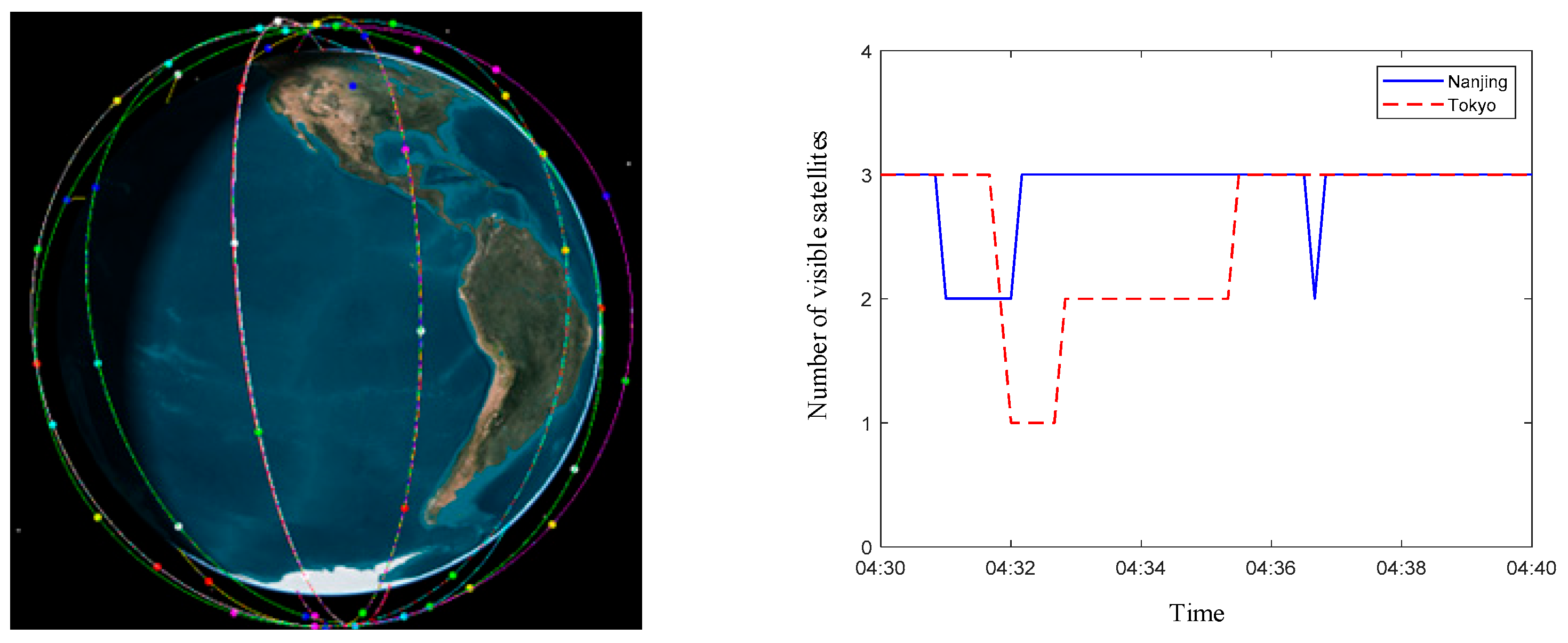
3.2. TDOA Positioning

Based on the previous section’s analysis of the time-delay and Doppler observations of the NPSS in the satellite channel, this section utilizes these time-delay observations to establish a TDOA equation for determining the terminal’ s position.

In this study, we focus on NB-IoT terminal positioning within the Iridium satellite constellation, which consists of 66 satellites in polar orbits. Figure 6 shows the number of visible satellites within a 10-min period for different regions under the Iridium constellation. From the figure, it is clear that the terminal is able to see three or two satellites for most of the time, while occasionally seeing only one satellite. Therefore, we categorize the research into three scenarios based on the number of visible satellites.

Under the Iridium constellation, the time differences between signals received from multiple visible satellites are typically within 5 ms, which is smaller than the NPSS period of 10 ms. Thus, the terminal only needs to detect the number of NPSSs received within one cycle to determine the number of visible satellites.

TDOA is a positioning algorithm which requires only three satellite observation points and their corresponding signal arrival times at the terminal to establish the necessary equations for positioning. Our research focuses on the selection of satellite observation points and the estimation of signal arrival times.

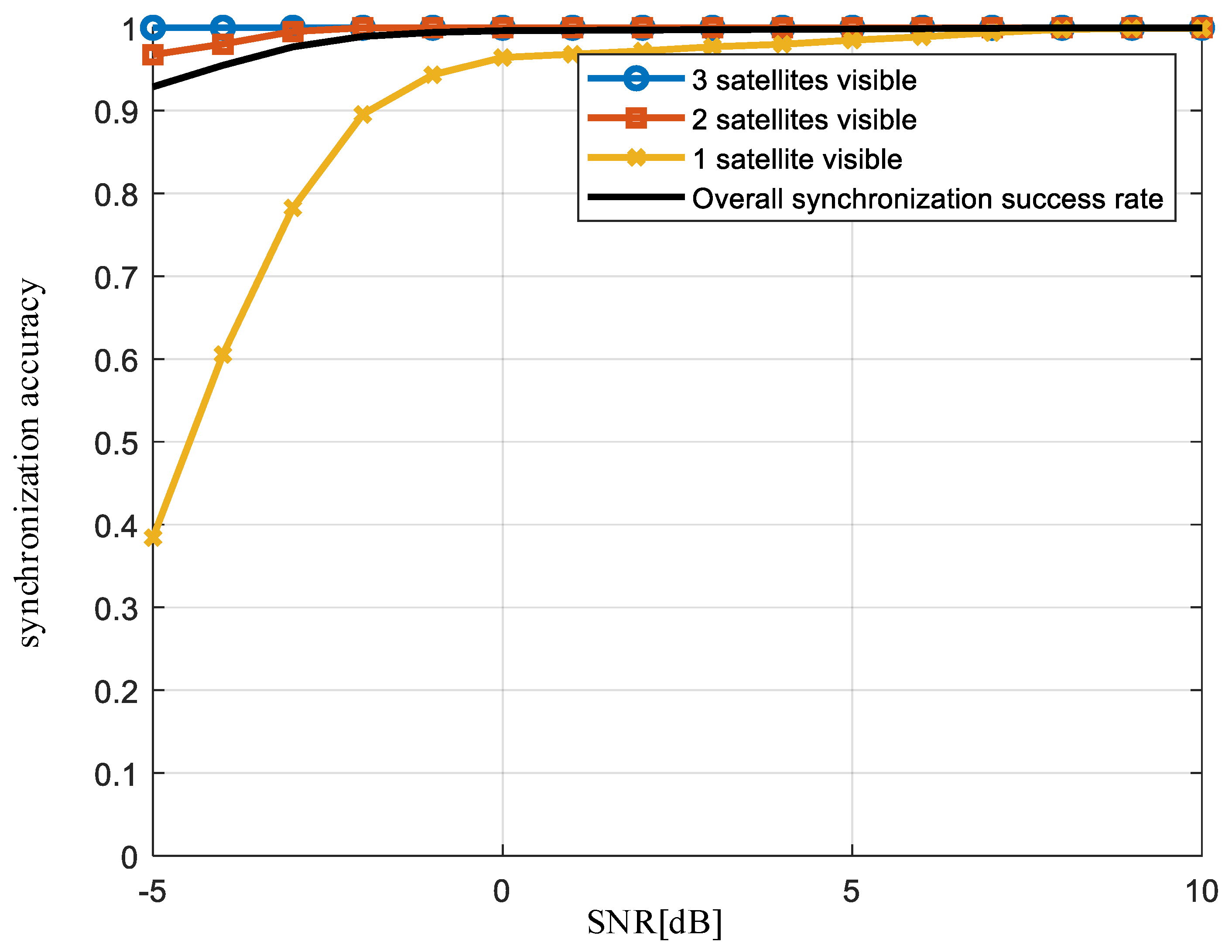
3.2.1. Scenario 1: Three Satellites Visible

In the scenario shown in Figure 7, the ground terminal $q=(x,y,z)$ can observe three satellites: $S_1$, $S_2$, and $S_3$. When there is a need for data upload, the terminal begins by utilizing the MSA algorithm from the previous section to detect the downlink NPSS. Once the first NPSS is detected, the terminal then detects two additional NPSSs within 10 ms, confirming that the scenario involves three visible satellites. The terminal records the arrival times of the three NPSSs and the satellite ephemeris to formulate the TDOA equations. The NB-IoT terminal must be equipped with an elevation sensor to incorporate surface constraints.

The distances from the three low earth orbit satellites $S_1$, $S_2$, and $S_3$ to the ground terminal are denoted as $r_1,r_2,r_3$:

$$\left\{\begin{array}{l}{r}_1=\left|s_1-q\right|=\sqrt{{(x_1-x)}^2+{(y_1-y)}^2+{(z_1-z)}^2}\\ r_2=\left|s_2-q\right|=\sqrt{{(x_2-x)}^2+{(y_2-y)}^2+{(z_2-z)}^2}\\ r_3=\left|s_3-q\right|=\sqrt{{(x_3-x)}^2+{(y_3-y)}^2+{(z_3-z)}^2}\end{array}\right.$$

(17)

Here, $\left(x_i,y_i,z_i\right)$ represents the coordinate values of satellite $S_i$. Let $\Delta t_1,\Delta t_2$ represent the time differences between the arrival times of the second and third NPSSs detected by the NB-IoT terminal, relative to the first NPSS’s arrival time. Let $\Delta r_2,\Delta r_3$ represent the distance differences at the time of signal transmission between the second and third satellites and the first satellite to the ground terminal, respectively. The distance difference equations can be written as:

$$\Delta r_i=r_i-r_1=c\cdot \Delta t_i,i=2,3$$

(18)

where $c$ is the speed of electromagnetic wave propagation. Assuming a spherical Earth model, the radius of the Earth and the altitude of the NB-IoT terminal are denoted by $R$ and $h_n$. Figure 8 illustrates the receiver timeline, where $L_1,L_2,L_3$ represent the arrival times of the three NPSSs.

$\Delta t_1$ denote the time difference of arrival between the signals transmitted from satellite $S_1$ and satellite $S_2$, $\Delta t_2$ denote the time difference of arrival between the signals transmitted from satellite $S_1$ and satellite $S_3$. They are respectively denoted as:

$$\Delta t_1=L_2-L_1\Delta t_2=L_3-L_1$$

(19)

Thus, the following TDOA equations can be derived, including the surface constraints which the terminal coordinates satisfy and the spherical equation of the earth:

$$\left\{\begin{array}{l}{r}_2-r_1=c\Delta t_1\\ r_3-r_1=c\Delta t_2\\ x^2+y^2+z^2={(R+h_n)}^2\end{array}\right.$$

(20)

Substituting Equations (17) and (18) and squaring both sides yields:

$$\Delta r_i^2+2\Delta r_i{r}_1+r_1^2={(R+h_n)}^2+s_i^T{s}_i-2s_i^{T}q,i=2,3$$

(21)

From the first equation in the system of equations, we obtain:

$$r_1^2={(R+h_n)}^2+s_1^T{s}_1-2s_1^{T}q$$

$$\Delta r_i^2+2\Delta r_i{r}_1=s_i^T{s}_i-s_1^T{s}_1-2{(s_i-s_1)}^{T}q,i=2,3$$

(22)

During the solving process, it is necessary to first express $q$ in terms of a linear expression of $r_1$ and then use Equation (22) to solve for $r_1$. Ultimately, the solution for $q$ in terms of $r_1$ is obtained as:

$$\widehat{q}=G_1^{-1}{G}_2$$

(23)

where

$$G_1=-2\left[\begin{array}{l}{s}_1^T\\ s_2^T-s_1^T\\ s_3^T-s_1^T\end{array}\right],G_2=\left(\begin{array}{ccc}-(R+h_n{)}^2-s_1^T{s}_1& 0& 1\\ \Delta r_1^2-s_2^T{s}_2+s_1^T{s}_1& 2\Delta r_1& 0\\ \Delta r_2^2-s_3^T{s}_3+s_1^T{s}_1& 2\Delta r_2& 0\end{array}\right)\left(\begin{array}{l}1\\ r_1\\ r_1^2\end{array}\right)$$

(24)

3.2.2. Scenario 2: Dual Satellite Visibility

In the Scenario depicted in Figure 9, when the terminal detects only one additional NPSS within 10 ms after detecting the first NPSS, it can conclude that the system is in a dual-satellite visible scenario. At this point, there are fewer visible satellites, and the terminal is unable to immediately calculate its position. The terminal records the arrival times of the NPSSs, denoted as $L_1$ and $L_2$, and the satellite real-time ephemeris $S_1(x_1,y_1,z_1)$, $S_2(x_2,y_2,z_2)$. It then enters the Power Saving Mode (PSM) for a duration of $T$. After the PSM sleep period, the terminal re-detects the NPSSs. If three satellites are now visible, it directly uses the method from the three-satellite visible scenario to calculate the position. If the three-satellite visible scenario is not detected, the terminal records the arrival time $L_3$ of the first NPSS and the satellite ephemeris $S_3(x_3,y_3,z_3)$. The time difference for the dual-satellite visible scenario is given by:

$$\begin{array}{l}\Delta t_1=L_2-L_1\\ \Delta t_2=L_3-L_1-T\end{array}$$

(25)

In dual-satellite and single-satellite visible scenarios, it is necessary to detect downlink satellite signals at different time instances in order to obtain observational values. The longer the interval between observations, the better the geometric configuration of the satellites becomes, resulting in higher positioning accuracy. However, NB-IoT terminals are power-constrained IoT devices, operating in four general power states: transmission, reception, light sleep, and deep sleep. Between two consecutive signal detection events for acquiring observations, the terminal must enter deep sleep mode for a prolonged interval denoted as $T$. A longer observation interval $T$ leads to higher energy consumption and longer synchronization latency but improves positioning accuracy. Conversely, a shorter $T$ reduces power consumption but may result in insufficient positioning and TA estimation accuracy, potentially failing to meet the synchronization requirements for NB-IoT uplink. Therefore, depending on the accuracy requirements, each terminal can adaptively adjust its observation interval $T$ to strike a balance between positioning accuracy and power consumption. To ensure better satellite geometry for localization, this paper sets 100 s.

Accordingly, the TDOA equations with surface constraints can be formulated as:

$$\left\{\begin{array}{l}{r}_2-r_1=c\Delta t_1\\ r_3-r_1=c\Delta t_2\\ x^2+y^2+z^2={(R+h_n)}^2\end{array}\right.$$

(26)

The terminal’s coordinates can be determined using the method outlined earlier.

3.2.3. Scenario 3: Single-Satellite Visibility

In the scenario shown in Figure 10, if no additional NPSSs are detected within 10 ms after the reception of the first NPSS, the terminal determines that it is in a single-satellite visibility scenario. In this case, the terminal records the arrival time of the NPSS as $L_1$ and the corresponding satellite ephemeris as $S_1(x_1,y_1,z_1)$, then enters PSM for a duration of $T$ seconds. After exiting PSM, the terminal performs another NPSS detection. If three satellites are detected at that time, the terminal directly applies the method described in Scenario 1 for positioning. If only two satellites are detected, the terminal records the arrival times of the two NPSSs as $L_2,L_3$ and combines this information with the previously recorded arrival time $L_1$ and satellite ephemeris $S_1(x_1,y_1,z_1)$ to perform the positioning calculation. In this case, the observation value a is given by:

$$\begin{array}{l}\Delta t_1=L_2-L_1-T\\ \Delta t_2=L_3-L_1-T\end{array}$$

(27)

If the terminal still detects only a single satellite at this time, it records the arrival time of the NPSS as $L_2$ and the corresponding satellite ephemeris as $S_2(x_2,y_2,z_2)$, then re-enters PSM for another duration of $T$ seconds. Upon waking, the terminal repeats the above procedure. If the single-satellite visibility condition persists, it records the NPSS arrival time as $L_3$ and the satellite ephemeris as $S_3(x_3,y_3,z_3)$. The observation value at this point is given by:

$$\begin{array}{l}\Delta t_1=L_2-L_1-T\\ \Delta t_2=L_3-L_1-2T\end{array}$$

(28)

Substituting into Equation (23), the terminal coordinates can be obtained. The entire TDOA positioning process is presented in Algorithm 2.

Algorithm 2: TDOA Localization Algorithm

Input: Satellite positions, NPSS detection time within 10 ms, detection interval time $T$.

Output: Terminal location.

1: Initialize

2: Detect the number of NPSSs $K$ within 10 ms, record the arrival time $L_i$

3:   While $K=3$, do

4:    Calculate $\Delta t_1,\Delta t_2$ using Formula (19) and Obtain $\widehat{q}=G_1^{-1}h$ using Formula (23);

5:   While $K=2$, do

6:    Record the arrival time $L_1,L_2$, enter PSM mode for $T$ time then update $K$;

7:    Jump to step 3 if $K=3$, record the first arrival time $L_3$;

8:    Calculate $\Delta t_1,\Delta t_2$ using Formula (25) and obtain $\widehat{q}$ using Formula (23);

9:   While $K=1$, do

10:    Record the arrival time $L_1$, enter PSM mode for $T$ time, then update $K$;

11:     Jump to step 3 if $K=3$, calculate $\Delta t_1,\Delta t_2$ using Formula (27), and obtain $\widehat{q}$ using Formula (25) if $K=2$;

12:   Record the arrival time $L_2$, enter PSM mode for $T$ time then update $K$;

13:     Jump to step 3 if $K=3$, record the arrival time $L_3$, calculate $\Delta t_1,\Delta t_2$ using Formula (28), and obtain $\widehat{q}$ using Formula (23);

14:   End

3.3. Error Analysis

This paper adopts the Root Mean Squared Error (RMSE) of the positioning error to evaluate performance. The position of the NB-IoT terminal is represented by $q$, and the positioning error can be denoted as $RMSE=\sqrt{E[(\widehat{q}-q){(\widehat{q}-q)}^T]}$.

The following derivation presents the CRLB of the positioning error under the proposed NPSS detection algorithm. To simplify the analysis, it is assumed that the observations are independent and follow a Gaussian distribution. Define three satellites $s_1,s_2,s_3$ with coordinates $(x_1,y_1,z_1),(x_2,y_2,z_2),(x_3,y_3,z_3)$. The distances between the three satellites and the unknown position $q$ with coordinates $(x,y,z)$ is denoted as $r_1,r_2,r_3$, respectively. Let $\Delta t_1,\Delta t_2$ represent the time differences of arrival between signals transmitted by $s_1,s_2$ and satellites $s_1,s_3$. The corresponding observation model can be expressed as:

$$\begin{array}{l}\Delta t_1={\displaystyle \frac{r_2-r_1}{c}}+{\lambda }_1\\ \Delta t_2={\displaystyle \frac{r_3-r_1}{c}}+{\lambda }_2\end{array}$$

(29)

where $c$ denotes the speed of light, and ${\lambda }_1,{\lambda }_2$ represent observational errors assumed to follow a Gaussian distribution. $r_1,r_2,r_3$ can be expressed as:

$$\left\{\begin{array}{l}{r}_1=\left|s_1-n\right|=\sqrt{{(x_1-x)}^2+{(y_1-y)}^2+{(z_1-z)}^2}\\ r_2=\left|s_2-n\right|=\sqrt{{(x_2-x)}^2+{(y_2-y)}^2+{(z_2-z)}^2}\\ r_3=\left|s_3-n\right|=\sqrt{{(x_3-x)}^2+{(y_3-y)}^2+{(z_3-z)}^2}\end{array}\right.$$

(30)

Define the parameter vector $\theta =[x,y,z]$. Since $q$ is subject to the surface constraint, it satisfies $z=\sqrt{R^2-x^2-y^2}$. Accordingly, the parameter vector can be redefined as $\theta =[x,y]$. The observation vector is denoted by $\mu =[{\mu }_1,{\mu }_2]$, and the measurement equation is given by $\mu =g(\theta )+\lambda$, where

$$\begin{array}{ll}g\left(\theta \right)=& [\sqrt{{\left(x_2-x\right)}^2+{\left(y_2-y\right)}^2+{\left(z_2-z\right)}^2}-\sqrt{{\left(x_1-x\right)}^2+{\left(y_1-y\right)}^2+{\left(z_1-z\right)}^2},\\ & \sqrt{{\left(x_3-x\right)}^2+{\left(y_3-y\right)}^2+{\left(z_3-z\right)}^2}-\sqrt{{\left(x_1-x\right)}^2+{\left(y_1-y\right)}^2+{\left(z_1-z\right)}^2}]/c\end{array}$$

(31)

Next, we compute the Jacobian matrix $J$, where the element in the $i$ row and $j$ column is denoted as ${\displaystyle \frac{\partial g_i}{\partial {\theta }_j}}$. The Jacobian matrix can then be expressed as:

$$J=\left(\begin{array}{cc}{\displaystyle \frac{\partial g_1}{\partial x}}& {\displaystyle \frac{\partial g_1}{\partial y}}\\ {\displaystyle \frac{\partial g_2}{\partial x}}& {\displaystyle \frac{\partial g_2}{\partial y}}\end{array}\right)$$

(32)

The Fisher Information Matrix $I$ is computed:

$$I=J^T\cdot {\beta }^{-1}\cdot J$$

(33)

Here, $\beta$ denotes the covariance matrix of the observation noise. The observation errors are assumed to be independent and follow a Gaussian distribution. As a result, $\beta$ is a diagonal matrix, with its diagonal elements representing the variances of the observation errors:

$$\beta =\left(\begin{array}{cc}{\rho }^2& 0\\ 0& {\rho }^2\end{array}\right)$$

(34)

Finally, the Cramér–Rao lower bound is given by the diagonal elements of the inverse of the Fisher Information Matrix $I$:

$$CRLB=\sqrt{trace(I^{-1})}$$

(35)

The CRLB is compared with the RMSE to verify the positioning performance. After completing the positioning, the terminal needs to estimate the TA and perform Doppler frequency offset pre-compensation using satellite ephemeris and its own position to complete the entire uplink synchronization process. $U_{\widehat{n}-sat}$ represents the distance from the computed position $\widehat{q}$ to the satellite; $U_{n-sat}$ represents the distance from the true position $q$ to the satellite; and $\Delta U$ denotes the difference between $U_{\widehat{n}-sat}$ and $U_{n-sat}$. To ensure that the uplink signal from each terminal received by the satellite falls within the range of one CP, $\Delta U$ should satisfy:

$$\Delta U=\left|U_{n-sat}-U_{\widehat{n}-sat}\right|\le (cp/2)\cdot c$$

(36)

In this paper, the length of the cyclic prefix is taken as one-quarter of the OFDM symbol length, and the calculated target value is approximately 2500 m:

$$\Delta U\le 2500 \mathrm{m}$$

(37)

When the distance between the position obtained after localization and the satellite is less than 2500 m compared to the true distance from the position to the satellite, the NB-IoT terminal can correctly complete the uplink synchronization based on the computed TA value and pre-compensated Doppler frequency offset.

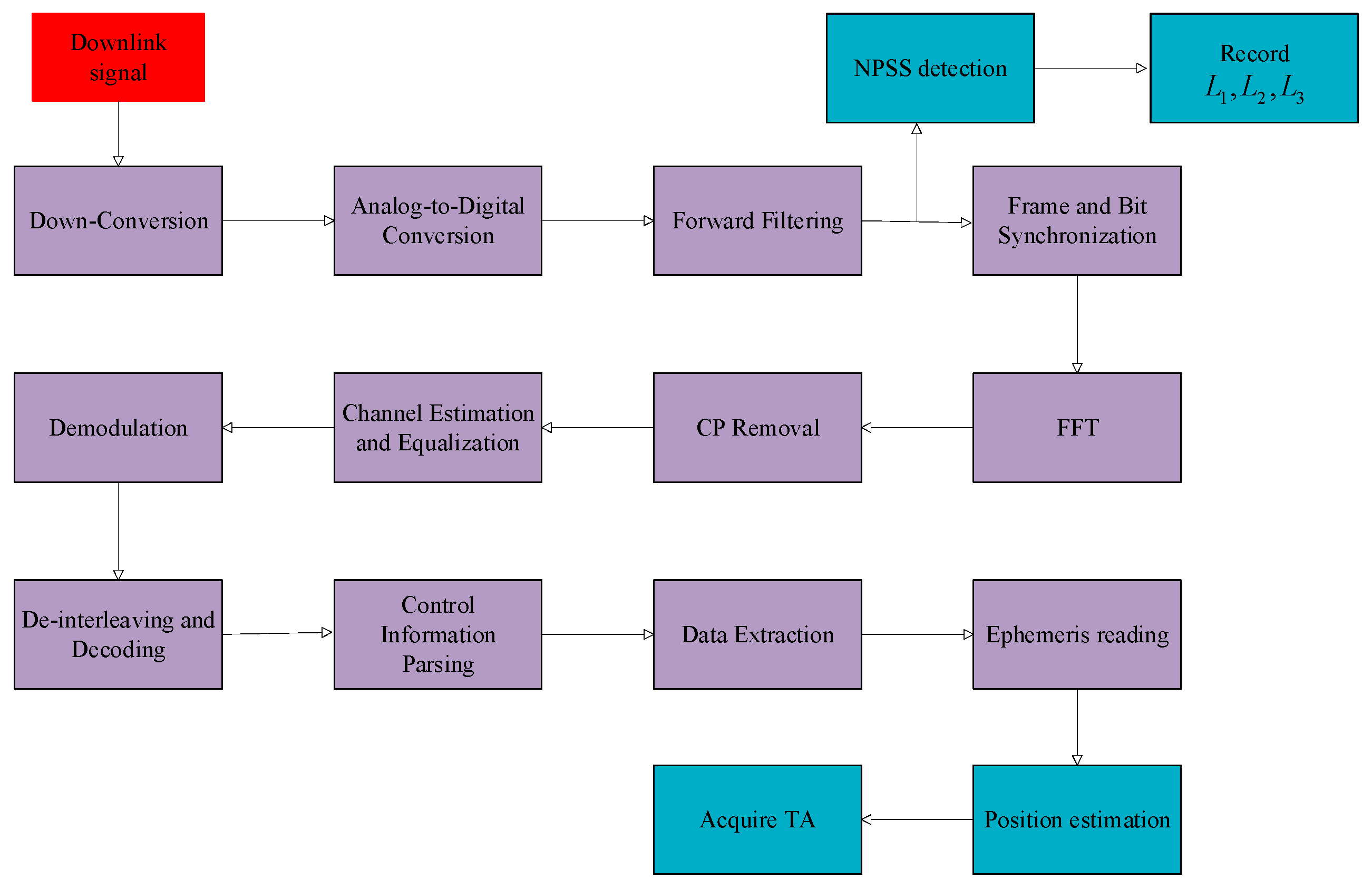
3.4. Receiver Architecture

Considering the engineering design requirements, this paper proposes the architecture of an NB-IoT terminal receiver for satellite communication using the BOS method in Figure 11. After down-conversion, analog-to-digital conversion (ADC), and forward filtering, the received signal undergoes frame synchronization using the NPSS detection method outlined in this paper. During this process, observation values $L_1,L_2,L_3$ are recorded. After performing FFT to remove the CP of the OFDM symbols, channel equalization and estimation are carried out. Data is demodulated and decoded to extract satellite ephemerides, and the TDOA algorithm proposed in this paper is used for position estimation. Finally, the TA value is calculated to complete the uplink synchronization.

3.5. Energy Consumption and Algorithm Complexity Analysis

For NB-IoT terminals, power consumption is a critical metric in evaluating performance. The uplink synchronization algorithm based on position assistance proposed in this paper can serve as an alternative to GNSS. To validate its superiority in terms of power consumption, this section compares the power consumption generated by this uplink synchronization scheme without external system assistance to that of GNSS-assisted uplink synchronization. According to the power consumption study in [14], the power consumption caused by computations during the uplink synchronization process has negligible impact on the battery life, with the primary determinant of power consumption being the duration of the NB terminal’s states.

For simplicity, this paper classifies the NB terminal’s states into reception, transmission, light sleep, and PSM. As pointed out in the 3GPP report, the workflow for a terminal using a GNSS-based solution is as follows:

In Figure 12, before transmitting uplink data, the terminal needs to perform GNSS positioning, and during the GNSS positioning process, the Radio Resource Control (RRC) connection must be disconnected. According to data from the 3GPP standard, this portion of the power consumption accounts for 30–50% of the UE’s total power consumption. By utilizing its own signals for positioning calculations, the terminal can save a significant amount of power during this process. Although the positioning accuracy of GNSS is higher than that of the BOS method, NB terminals do not require such high positioning accuracy to successfully complete uplink synchronization. For IoT terminals of this type, the solution presented in this paper is more valuable. The following section provides a detailed analysis of the states and duration of the NB terminal during the uplink synchronization process in both solutions, followed by a power consumption comparison analysis.

Power Consumption Analysis of the BOS Method: Assuming that an IoT terminal reports data at a 2-h reporting interval, this section analyzes the terminal’s state transitions and computes the corresponding power consumption according to the NB-IoT protocol. Finally, the results are compared with those of the GNSS-based method.

The total power consumption of the BOS-based scheme can be expressed as:

$$E_{BOS}=E_{sync}+E_{RA}+E_{UL}+E_{DRX}+E_{PSM}+E_{extra}$$

(38)

$E_{RA}=P_{TX}(T_{msg1}+T_{msg3})+P_{RX}(T_{msg2}+T_{msg4})+2P_{DRX}{T}_{RTT}$ denotes the energy consumed during the random access;$E_{UL}=P_{TX}{T}_{date}+P_{DRX}{T}_{RTT}$ refers to the energy consumed during uplink data transmission; $E_{DRX}=P_{DRX}(T_{DRX}-T_{PO})+P_{RX}{T}_{PO}$ denotes the energy consumed in DRX; $E_{PSM}=P_{PSM}(T_{PSM}-T_{DRX})$ denotes the energy consumed in PSM; $E_{extra}$ indicates the power consumption of the barometric altitude sensor; and $E_{sync}=P_{RX}{T}_{sync}$ represents the energy consumed by the NB-IoT terminal during downlink synchronization and terminal positioning using the proposed method. The definitions and values of the remaining parameters are provided in

Table 1. Meaning and value of important notations.

Notation	Meaning	Value
$P_{TX}$	Transmission power	545 mW
$P_{RX}$	Reception power	90 mW
$P_{DRX}$	Power consumption during light sleep	3 mW
$P_{PSM}$	Power consumption during deep sleep	0.015 mW
$T_{msg1}$	Msg1 duration	0.01 s
$T_{msg2}$	Msg2 duration	0.01 s
$T_{msg3}$	Msg3 duration	0.01 s
$T_{msg4}$	Msg4 duration	0.01 s
$T_{RTT}$	RTT between UE and satellite	0.03 s
$T_{date}$	UL date duration	0.5 s
$T_{DRX}$	DRX cycle	1 s
$T_{PSM}$	PSM cycle	100 s
$E_{atti}$	Power consumption of elevation sensor	1 mW
$N_{GNSS}$	The number of GNSS satellites	4
$T_{GNSS-acq}$	GNSS acquisition duration	5–20 s
$T_{GNSS-track}$	GNSS tracking duration	1 s

.

Power Consumption Analysis of the GNSS-based Method:

$$\begin{array}{ll}{E}_{GNSS}=& P_{RX}(T_{GNSS-acq}+N_{GNSS}{T}_{GNSS-track})\\ & +N_{GNSS}(E_{sync’}+E_{RA})+E_{UL}\\ & +E_{DRX}+E_{PSM}\end{array}$$

(39)

The definitions and values of all parameters involved are listed in Table 1. A detailed comparative simulation analysis of the power consumption for both schemes is presented in the next section.

We analyze the algorithm complexity in

Table 2. Comparison of algorithm complexity.

Algorithm	Complexity
MSA	$O\left(1.39e^6\cdot n\right)$
Maximum Likelihood	$O\left(1.04e^6\cdot n\right)$

. In the MSA, the main computational burden comes from complex multiplications during correlation operations as well as a large number of complex multiplications involved in the FFT process. In contrast, the maximum likelihood algorithm only involves complex multiplications during correlation. The final results show that MSA incurs approximately 33% more computational cost compared to the conventional algorithm.

4. Simulation Analysis

The accuracy of the NPSS detection algorithm directly affects the acquisition of TDOA observation values and the subsequent synchronization precision. Figure 13 compares the detection performance of the proposed MSA algorithm with the maximum likelihood (ML) algorithm under various signal-to-noise ratios and Doppler frequency offsets. The results indicate that the MSA algorithm can achieve a timing error within one symbol duration even under negative SNR conditions and maintains reliable detection performance under severe Doppler shifts. Although the MSA algorithm demonstrates superior detection capability compared to the ML algorithm, it incurs a higher computational complexity.

Figure 14 presents the distribution of uplink TA estimation errors under different SNR conditions for three distinct scenarios using the proposed BOS scheme. In the three-satellite and two-satellite visibility cases, favorable satellite geometry results in lower positioning errors and narrower TA ambiguity ranges, allowing successful uplink synchronization even at low SNR levels. However, in the single-satellite scenario, the weak satellite geometry significantly degrades positioning accuracy, causing the BOS scheme to reach the threshold of acceptable TA estimation accuracy at around −4 dB. Nevertheless, single-satellite visibility is relatively rare in the Iridium constellation and thus does not significantly impact the overall performance of the BOS approach.

Figure 15 illustrates the uplink synchronization success rates under different visible satellite scenarios. In the Iridium constellation, the proportions of triple-satellite, dual-satellite, and single-satellite visibility are approximately 6:3:1. Based on this distribution, the proposed scheme achieves an uplink synchronization success rate of 98% even under negative SNR conditions.

Figure 16 compares the RMSE of the proposed TDOA-based positioning method with the CRLB. The results demonstrate that the proposed method achieves positioning accuracy close to the CRLB under low SNR conditions, indicating its effectiveness as a reliable localization approach.

Figure 17 shows the positioning error over a 50-min period in the Nanjing and Tokyo regions under an SNR of −2 dB using the proposed algorithm. It can be observed that while the error fluctuates significantly over different time windows, it generally remains around 200 m. Figure 18 illustrates the impact of the NB terminal’s sleep duration $T$ on TA estimation under the dual-satellite visibility scenario. A clear negative correlation is observed. However, an excessively large $T$ value would increase power consumption during the synchronization process. Therefore, we choose 100 s as the sleep duration.

Figure 19 presents a comparison of energy consumption between the GNSS-based scheme and the proposed BOS scheme under different satellite visibility scenarios. It is evident that the GNSS-based approach incurs significantly higher energy consumption compared to the BOS scheme. The three-satellite case exhibits the lowest power consumption, as only a single measurement is required to complete uplink synchronization. Overall, the BOS scheme achieves an energy saving of approximately 15% to 40% compared to the GNSS-based method.

5. Conclusions

In this paper, we propose a new uplink synchronization method for NB-IoT by calculating the terminal’s TA value and achieving uplink synchronization through detection of the NPSS broadcasted by satellites. To address the significant Doppler frequency shifts present in LEO satellites, an MSA algorithm is designed to enhance NPSS detection performance by exploiting the symmetry of NPSSs. An additional 33% increase in computational complexity results in improved NPSS detection performance. TDOA equations are established for different visible satellite scenarios, and uplink synchronization is achieved by combining terminal self-positioning with satellite ephemeris. Finally, compared to traditional GNSS-assisted approaches, the method proposed in this paper lowers terminal power consumption by 15–40% and maintains an uplink synchronization success rate exceeding 98%, even in negative SNR environments.

At present, our work remains at the simulation level. In the future, we plan to investigate its feasibility at the hardware level.

References

1. Yang, M.; Dong, X.; Hu, M. Design and simulation for hybrid LEO communication and navigation constellation. In Proceedings of the 2016 IEEE Chinese Guidance, Navigation and Control Conference (CGNCC), Nanjing, China, 12–14 August 2016; pp. 1665–1669. [Google Scholar]
2. Vaezi, M.; Azari, A.; Khosravirad, S.R.; Shirvanimoghaddam, M.; Azari, M.M.; Chasaki, D.; Popovski, P. Cellular, wide-area, and non-terrestrial IoT: A survey on 5G advances and the road toward 6G. IEEE Commun. Surv. Tutor. 2022, 24, 1117–1174. [Google Scholar] [CrossRef]
3. Lin, J.; Hou, Z.; Zhou, Y.; Tian, L.; Shi, J. Map estimation based on Doppler characterization in broadband and mobile LEO satellite communications. In Proceedings of the 2016 IEEE 83rd Vehicular Technology Conference (VTC Spring), Nanjing, China, 15–18 May 2016; pp. 1–5. [Google Scholar]
4. Hu, D.; Song, C. Design of the inter satellite link of low earth orbit mobile satellite communication systems. Radio Commun. Technol. 2017, 43, 11–15. [Google Scholar]
5. Wang, A.; Wang, P.; Miao, X.; Li, X.; Ye, N.; Liu, Y. A review on non-terrestrial wireless technologies for smart city Internet of Things. Int. J. Distrib. Sens. Netw. 2020, 16, 1550147720936824. [Google Scholar] [CrossRef]
6. Wang, W.; Liu, A.; Zhang, Q.; You, L.; Gao, X.Q.; Zheng, G. Robust multigroup multicast transmission for frame-based multi-beam satellite systems. IEEE Access 2018, 6, 46074–46083. [Google Scholar] [CrossRef]
7. You, L.; Li, K.-X.; Wang, J.; Gao, X.Q.; Xia, X.-G.; Ottersten, B. Massive MIMO transmission for LEO satellite communications. IEEE J. Sel. Areas Commun. 2020, 38, 1851–1865. [Google Scholar] [CrossRef]
8. Kapovits, A.; Corici, M.I.; Gheorghe-Pop, I.D.; Gavras, A.; Burkhardt, F.; Schlichter, T.; Covaci, S. Satellite communications integration with terrestrial networks. China Commun. 2018, 15, 22–38. [Google Scholar] [CrossRef]
9. Pardhasaradhi, B.; Srinath, G.; Raghu, J.; Srihari, P. Position estimation in indoor using networked GNSS sensors and a range-azimuth sensor. Inf. Fusion. 2023, 89, 189–197. [Google Scholar] [CrossRef]
10. Zhang, L.; Zhang, T.; Shin, H.-S. An efficient constrained weighted least squares method with bias reduction for TDOA-based localization. IEEE Sens. J. 2021, 21, 10122–10131. [Google Scholar] [CrossRef]
11. Zhu, F.; Ba, T.; Zhang, Y.; Gao, X.; Wang, J. Terminal location method with NLOS exclusion based on unsupervised learning in 5G-LEO satellite communication systems. Int. J. Satell. Commun. Netw. 2020, 38, 425–436. [Google Scholar] [CrossRef]
12. Lin, X.; Lin, Z.; Löwenmark, S.E.; Rune, J.; Karlsson, R. Doppler shift estimation in 5G new radio non-terrestrial networks. In Proceedings of the 2021 IEEE Global Communications Conference (GLOBECOM), Madrid, Spain, 7–11 December 2021; pp. 1–6. [Google Scholar]
13. Kodheli, O.; Astro, A.; Querol, J.; Gholamian, M.; Kumar, S.; Maturo, N.; Chatzinotas, S. Random access procedure over non-terrestrial networks: From theory to practice. IEEE Access 2021, 9, 109130–109143. [Google Scholar] [CrossRef]
14. Janssen, T.; Koppert, A.; Berkvens, R.; Weyn, M. A survey on IoT positioning leveraging LPWAN, GNSS, and LEO-PNT. IEEE Internet Things J. 2023, 10, 11135–11159. [Google Scholar] [CrossRef]
15. Wang, W.; Chen, T.; Ding, R.; Seco-Granados, G.; You, L.; Gao, X. Location-based timing advance estimation for 5G integrated LEO satellite communications. IEEE Trans. Veh. Technol. 2021, 70, 6002–6017. [Google Scholar] [CrossRef]
16. Chandrika, V.R.; Chen, J.; Lampe, L.; Vos, G.; Dost, S. SPIN: Synchronization signal-based positioning algorithm for IoT nonterrestrial networks. IEEE Internet Things J. 2023, 10, 20846–20867. [Google Scholar] [CrossRef]
17. Wei, Q.; Chen, X.; Ni, Z.; Jiang, C.; Huang, Z.; Zhang, S. Integrated Doppler positioning in a narrowband satellite system: Performance bound, parameter estimation, and receiver architecture. IEEE Internet Things J. 2024, 11, 10893–10910. [Google Scholar] [CrossRef]
18. Xv, H.; Sun, Y.; Zhao, Y.; Peng, M.; Zhang, S. Joint beam scheduling and beamforming design for cooperative positioning in multi-beam LEO satellite networks. IEEE Trans. Veh. Technol. 2024, 73, 5276–5287. [Google Scholar] [CrossRef]
19. Tao, T. Research on Positioning and Downlink Synchronization Technology of Low Earth Orbit Satellite Mobile Communication. Master’s Thesis, Southeast University, Nanjing, China, 2019. [Google Scholar]
20. Tong, Y. Design of Time-Frequency Synchronization Technology for 5G Integrated Low Earth Orbit Satellite Mobile Communication Systems. Master’s Thesis, Southeast University, Nanjing, China, 2019. [Google Scholar]
Figure 1. Illustration of LEO and GNSS satellite-based IoT network.
Symmetry 17 00984 g001
Figure 2. NPSS structure diagram.
Symmetry 17 00984 g002
Figure 3. Flowchart of the MSA algorithm.
Symmetry 17 00984 g003
Figure 4. Computation diagram for different m values.
Symmetry 17 00984 g004
Figure 5. Illustrations of three sampling point distributions.
Symmetry 17 00984 g005
Figure 6. Iridium satellite constellation diagram.
Symmetry 17 00984 g006
Figure 7. Three-satellite visible scenario diagram.
Symmetry 17 00984 g007
Figure 8. Receiver timing diagram.
Symmetry 17 00984 g008
Figure 9. Two-satellite visibility scenario diagram.
Symmetry 17 00984 g009
Figure 10. Single-satellite visibility scenario diagram.
Symmetry 17 00984 g010
Figure 11. Receiver architecture diagram.
Symmetry 17 00984 g011
Figure 12. GNSS system flowchart.
Symmetry 17 00984 g012
Figure 13. Comparison diagram of NPSS detection algorithms.
Symmetry 17 00984 g013
Figure 14. Comparison of TA values under different scenarios.
Symmetry 17 00984 g014
Figure 15. Synchronization accuracy under different scenarios.
Symmetry 17 00984 g015
Figure 16. Comparison between positioning method and the Cramér–Rao lower bound.
Symmetry 17 00984 g016
Figure 17. Positioning accuracy at different times and in different regions.
Symmetry 17 00984 g017
Figure 18. Impact of different T values on TA estimation.
Symmetry 17 00984 g018
Figure 19. Power consumption comparison between proposed method and GNSS-based method.
Symmetry 17 00984 g019