Classes of Multivalent Spirallike Functions Associated with Symmetric Regions

Abstract

We define a function to unify the well-known class of Janowski functions with a class of spirallike functions of reciprocal order. We focus on the impact of defined function on various conic regions which are symmetric with respect to the real axis. Further, we have defined a new subclass of multivalent functions of complex order subordinate to the extended Janowski function. This work bridges the studies of various subclasses of spirallike functions and extends well-known results. Interesting properties have been obtained for the defined function class. Several consequences of our main results have been pointed out.

1. Introduction and Definitions

Let $\mathbb{N},\mathbb{R},$ and $\mathbb{C}$ represent the respective sets of natural numbers, real numbers, and complex numbers. For $p\in \mathbb{N}$, we let ${\mathcal{N}}_p$ denote the class of functions $\varphi$ of the form

$$\varphi \left(z\right)=z^p+\sum _{n=p+1}^{\infty }{a}_n{z}^n$$

(1)

which are analytic in the open unit disc $\mathbb{E}=\{z:z\in \mathbb{C}\mathrm{and}|z|<1\}$. We let $\mathcal{C}$ and ${\mathcal{S}}^{*}$ denote the well-known subclass of ${\mathcal{N}}_1$ which are convex and starlike in $\mathbb{E}$. Additionally, let $\mathcal{P}$ consist of functions $\chi$ which are analytic and is given by

$$\chi \left(z\right)=1+\sum _{n=1}^{\infty }{R}_n{z}^n,z\in \mathbb{E},R_1>0$$

(2)

and satisfies $Re\left(\chi \left(z\right)\right)>0$, $z\in \mathbb{E}$. For $-\pi /2<\sigma <\pi /2$, a function $\varphi \in {\mathcal{N}}_p$ is said to be $\sigma$-spiral in $\mathbb{E}$ if

$$Re\left\{e^{i\sigma }\frac{z{\varphi }^{\prime }\left(z\right)}{\varphi \left(z\right)}\right\}>0,(z\in \mathbb{E}).$$

(3)

Similarly, a function $\varphi \in {\mathcal{N}}_p$ is said to be convex $\sigma$-spiral in $\mathbb{E}$ if

$$Re\left\{e^{i\sigma }\left(1+\frac{z{\varphi }^{″}\left(z\right)}{{\varphi }^{\prime }\left(z\right)}\right)\right\}>0,(z\in \mathbb{E}).$$

(4)

We denote $\sigma$-spiral functions and convex $\sigma$-spiral functions, respectively, by ${\mathcal{SL}}_p\left(\sigma \right)$ and ${\mathcal{CS}}_p\left(\sigma \right)$.

The reciprocal class of $\sigma$-spiral functions was defined by Uyanik et al. in [1], by replacing $>0$ in the right hand side of the inequality (3) by $<\lambda$, $(\lambda >pcos\sigma )$. We denote the reciprocal class by ${\mathcal{RS}}_p(\sigma ,\lambda )$. Similar generalization was used to define reciprocal convex $\sigma$-spiral, by replacing $>0$ in the right hand side of the inequality (4) by $<\lambda$, $(\lambda >pcos\sigma )$ and is denoted by ${\mathcal{RC}}_p(\sigma ,\lambda )$. Further, it was established in [1] that the function $\varphi \left(z\right)\in R{S}_p(\sigma ,\lambda )$ if and only if

$$e^{i\sigma }\frac{z{\varphi }^{\prime }\left(z\right)}{\varphi \left(z\right)}\prec 2\lambda -p{e}^{-i\sigma }+\frac{2\left(pcos\sigma -\lambda \right)}{1-z},(z\in \mathbb{E}),$$

(5)

where $-\frac{\pi }{2}<\sigma <\frac{\pi }{2}$ and $\lambda >pcos\sigma$. Here ≺ denotes the usual subordination of analytic function. Similarly, $\varphi \in {\mathcal{N}}_p$ is said to be in ${\mathcal{RC}}_p(\sigma ,\lambda )$ if and only if it satisfies the condition

$$e^{i\sigma }\left(1+\frac{z{\varphi }^{″}\left(z\right)}{{\varphi }^{\prime }\left(z\right)}\right)\prec 2\lambda -p{e}^{-i\sigma }+\frac{2\left(pcos\sigma -\lambda \right)}{1-z},(z\in \mathbb{E}).$$

Purpose, Motivation and Novelty

The main purpose of this paper is to define a function ${\Delta }_{\sigma }^{\lambda }\left(z\right)$ (see (7)) so as to unify the superordinate function in (5) with the well-known class of Janowski functions. Our study would consolidate or unify the study of various subclasses related to spirallike and reciprocal spirallike functions.

Aouf [2] ([Equation 1.4]) defined the class $\mathcal{P}(U,V,p,\lambda )$ which consists of functions $h\left(z\right)=p+{\sum }_{n=1}^{\infty }{p}_n{z}^n$ analytic in the unit disc such that $h\left(z\right)\in \mathcal{P}(U,V,p,\lambda )$ if and only if

$$h\left(z\right)=\frac{p+\left[pV+(U-V)(p-\lambda )\right]w\left(z\right)}{\left[1+Vw\left(z\right)\right]},(-1\le V<U\le 1,0\le \lambda <1)$$

(6)

where $w\left(z\right)$ is the Schwartz function. The class $\mathcal{P}(U,V,p,\lambda )$ is an extension of the famous Janowski class of functions [3]. Motivated by the class recently studied by Breaz et al. [4] and in view of generalizing the superordinate function in (5), we now define and study the following relation

$$\begin{array}{c}{\Delta }_{\sigma }^{\lambda }\left(z\right)=\frac{\left[(1+U{e}^{-2i\sigma })p{e}^{i\sigma }+\lambda (V-U)\right]\chi \left(z\right)+\left[(1-U{e}^{-2i\sigma })p{e}^{i\sigma }-\lambda (V-U)\right]}{\left[(V+1)\chi \left(z\right)+(1-V)\right]},\end{array}$$

(7)

where $-1\le V<U\le 1,-\frac{\pi }{2}<\sigma <\frac{\pi }{2},\lambda >pcos\sigma$ and $\chi \left(z\right)\in \mathcal{P}$.

To study the impact of ${\Delta }_{\sigma }^{\lambda }\left(z\right)$ on various conic regions, we consider the following:

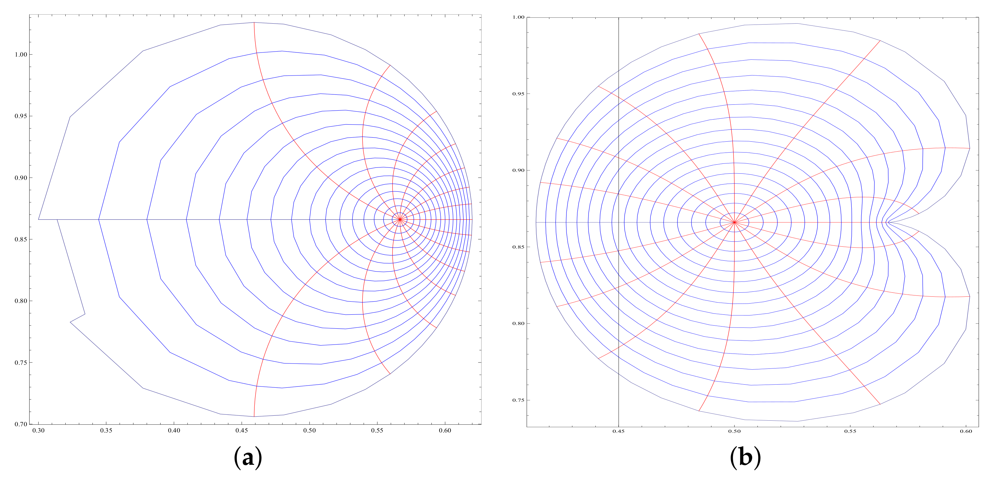
• $\chi \left(z\right)=\frac{1}{1-z}$ which maps unit disc onto the half plane $Re\left(w\right)>0.5$
• $\chi \left(z\right)=z^2+2z+2$ which maps the unit disc onto interior of the cardioid region with cusp on the left hand side

For an admissible choice of the parameter $U=0.5,V=-0.5$, $p=1,\sigma =\frac{\pi }{3}$ and $\lambda =0.6$, if the function

• $\chi \left(z\right)=\frac{1}{1-z}$, then ${\Delta }_{\sigma }^{\lambda }\left(z\right)$ maps the unit disc on to the interior of the circular domain (See Figure 1a).
  

  Figure 1. Impact of ${\Delta }_{\sigma }^{\lambda }\left(z\right)$ on the conic region $\chi \left(z\right)$ if $U=0.5,V=-0.5$, $p=1,\sigma =\frac{\pi }{3}$ and $\lambda =0.6$ (a) The image of the unit disc under the mapping of ${\Delta }_{\sigma }^{\lambda }\left(z\right)$, if $\chi \left(z\right)=1/1-z$. (b) The image of the unit disc under the mapping of ${\Delta }_{\sigma }^{\lambda }\left(z\right)$, if $\chi \left(z\right)=z^2+2z+2$.
• $\chi \left(z\right)=z^2+2z+2$, then ${\Delta }_{\sigma }^{\lambda }\left(z\right)$ maps unit disc onto a cardioid region which is magnified and the cusp of the cardioid gets rotated on to the right hand side (see Figure 1b).

Hence, the type of impact of ${\Delta }_{\sigma }^{\lambda }\left(z\right)$ on various regions is not the same.

Remark 1.

Now we will list some recent studies, which are special cases of ${\Delta }_{\sigma }^{\lambda }\left(z\right)$.

1

If we let $\sigma =0$ in (7), then ${\Delta }_{\sigma }^{\lambda }\left(z\right)$ reduces to

$$\aleph \left(z\right)=\frac{\left[(1+U)p+\lambda (V-U)\right]\chi \left(z\right)+\left[(1-U)p-\lambda (V-U)\right]}{\left[(V+1)\chi \left(z\right)+(1-V)\right]}.$$

The function $\aleph \left(z\right)$ was defined and studied by Breaz et al. in [4].

2

If we let $U=1,V=-1$ and $\chi \left(z\right)=(1+z)/(1-z)$ in (7), then ${\Delta }_{\sigma }^{\lambda }\left(z\right)$ reduces to $2\lambda -p{e}^{-i\sigma }+\frac{2\left(pcos\sigma -\lambda \right)}{1-z}$ (see the superordinate function in (5)).

For the function $\varphi \in {\mathcal{N}}_p$ given by (1) and $h\in {\mathcal{N}}_p$ of the form $h\left(z\right)=z^p+{\displaystyle \sum _{n=p+1}^{\infty }}{\Gamma }_n{z}^n$, the Hadamard product (or convolution) of these two function is defined by

$$\Omega \left(z\right):=(\varphi \ast h)\left(z\right):=z^p+\sum _{n=p+1}^{\infty }{a}_n{\Gamma }_n{z}^n,z\in \mathbb{E}.$$

(8)

Unless otherwise mentioned

$$-1\le V<U\le 1,\left|\sigma \right|<\frac{\pi }{2},\lambda >pcos\sigma .$$

Definition 1.

For $-{\displaystyle \frac{\pi }{2}}<\sigma <{\displaystyle \frac{\pi }{2}}$, $0\le \eta \le 1$, $\lambda \ge pcos\sigma$, $b\in \mathbb{C}\setminus \left\{0\right\}$ and $\Omega =\varphi \ast h$ defined as in (8), we say that the function ϕ belongs to the class ${\mathcal{LS}}_{\sigma }(\lambda ,\eta ;b;\chi ;h;U,V)$ if it satisfies the subordination condition

$$e^{i\sigma }\left[p+\frac{1}{b}\left\{\frac{\eta z^2{\Omega }^{″}\left(z\right)+[p(1-\eta )+\eta ]z{\Omega }^{\prime }\left(z\right)}{p(1-\eta )\Omega \left(z\right)+\eta z{\Omega }^{\prime }\left(z\right)}-p\right\}\right]\prec {\Delta }_{\sigma }^{\lambda }\left(z\right),$$

(9)

where “≺” denotes subordination and ${\Delta }_{\sigma }^{\lambda }\left(z\right)$ is defined as in (7).

Remark 2.

Recall that ${\mathcal{RS}}_p(\sigma ,\lambda )$ were defined as a generalization of the class ${\mathcal{RS}}_1(0,\lambda )$ introduced by Uralegaddi [5]. Further, the class ${\mathcal{RS}}_p(\sigma ,\lambda )$ was extended and studied by various authors (see [1,6,7,8,9,10]). Very recently, Altınkaya in [11] introduced and studied a new subclass of spirallike functions closely related to the defined function class ${\mathcal{LS}}_{\sigma }(\lambda ,\eta ;b;\chi ;h;U,V)$. We note that all the above mentioned studies can be obtained as special cases of our class ${\mathcal{LS}}_{\sigma }(\lambda ,\eta ;b;\chi ;h;U,V)$. The details of the special cases will be pointed out when we derive applications of our main results.

2. Preliminaries

Here, we prepare the groundwork that is required to obtain our main results. Firstly, we begin with the discussion of obtaining the Maclaurin series for the function ${\Delta }_{\sigma }^{\lambda }\left(z\right)$. From (7), we see that

$$\begin{array}{c}{\Delta }_{\sigma }^{\lambda }\left(z\right)=\frac{\left[\lambda (V-U)-(1-U{e}^{-2i\sigma })p{e}^{i\sigma }\right]}{(V-1)}\left[1-\frac{\left[(1+U{e}^{-2i\sigma })p{e}^{i\sigma }+\lambda (V-U)\right]\chi \left(z\right)}{\left[\lambda (V-U)-(1-U{e}^{-2i\sigma })p{e}^{i\sigma }\right]}\right]\\ \times {\left[1-\frac{(V+1)\chi \left(z\right)}{V-1}\right]}^{-1}\\ =\frac{\left[\lambda (V-U)-(1-U{e}^{-2i\sigma })p{e}^{i\sigma }\right]}{(V-1)}+\left\{\frac{\left[\lambda (V-U)-(1-U{e}^{-2i\sigma })p{e}^{i\sigma }\right](V+1)}{{(V-1)}^2}\right.-\\ \left.\frac{\left[(1+U{e}^{-2i\sigma })p{e}^{i\sigma }+\lambda (V-U)\right]}{(V-1)}\right\}\chi \left(z\right)\\ +\left\{\frac{\left[\lambda (V-U)-(1-U{e}^{-2i\sigma })p{e}^{i\sigma }\right]{(V+1)}^2}{{(V-1)}^3}-\frac{\left[(1+U{e}^{-2i\sigma })p{e}^{i\sigma }+\lambda (V-U)\right](V+1)}{{(V-1)}^2}\right\}{\left[\chi \left(z\right)\right]}^2+\cdots \\ =-\frac{2p{e}^{i\sigma }}{V-1}\left[1+\left(\frac{V+1}{V-1}\right)+{\left(\frac{V+1}{V-1}\right)}^2+\cdots \right]+\frac{2\left[U(p{e}^{-i\sigma }-\lambda )-V(p{e}^{i\sigma }-\lambda )\right]R_1}{{(V-1)}^2}\\ \left[1+2\left(\frac{V+1}{V-1}\right)+3{\left(\frac{V+1}{V-1}\right)}^2+\cdots \right]z+\cdots \\ =-\frac{2p{e}^{i\sigma }}{V-1}{\left[1-\left(\frac{V+1}{V-1}\right)\right]}^{-1}+\frac{2\left[U(p{e}^{-i\sigma }-\lambda )-V(p{e}^{i\sigma }-\lambda )\right]R_1}{{(V-1)}^2}{\left[1-\left(\frac{V+1}{V-1}\right)\right]}^{-2}z+\cdots \end{array}$$

Hence, (7) can be rewritten as

$${\Delta }_{\sigma }^{\lambda }\left(z\right)=p{e}^{i\sigma }+\frac{\left[U(p{e}^{-i\sigma }-\lambda )-V(p{e}^{i\sigma }-\lambda )\right]R_1}{2}z+\cdots$$

(10)

Remark 3.

In [12], Karthikeyan et al. have showed that convex function becomes starlike by varying the parameters in ${\Delta }_0^{\lambda }\left(z\right)$. Hence, the function ${\Delta }_{\sigma }^{\lambda }\left(z\right)$ may be convex univalent or starlike univalent depending on the function $\chi \left(z\right)$. It cannot be concluded that impact of ${\Delta }_{\sigma }^{\lambda }\left(z\right)$ on a convex region does not affect the convexity. However, if ${\Delta }_{\sigma }^{\lambda }\left(z\right)$ is to be convex univalent, it is always possible to find a function χ such that ${\Delta }_{\sigma }^{\lambda }\left(z\right)$ is convex univalent in $\mathbb{E}$. For example, if we choose $\chi \left(z\right)=\sqrt{1+z}$ then ${\Delta }_{\sigma }^{\lambda }\left(z\right)$ is convex univalent in $\mathbb{E}$ for all admissible values of the parameters involved. It is well-known that $\sqrt{1+z}$ is convex univalent in $\mathbb{E}$ (see Lemma 2.5 [13]), the function ${\Delta }_{\sigma }^{\lambda }\left(z\right)$ does not alter the conic $\sqrt{1+z}$ except for translation, magnification, and rotation. That is, it does not affect the convexity or univalence as we vary the parameters involved (see Figure 2a–d).

Figure 2. Impact of ${\Delta }_{\sigma }^{\lambda }\left(z\right)$ on the conic region $\chi \left(z\right)=\sqrt{1+z}$. (a) if $U=0.5,V=-0.5$, $p=1,\sigma =\frac{\pi }{3}$ and $\lambda =0.6$; (b) if $U=1,V=-1$, $p=1,\sigma =\frac{\pi }{3}$ and $\lambda =0.6$; (c) if $U=1,V=-1$, $p=2,\sigma =\frac{\pi }{3}$ and $\lambda =0.6$; (d) if $U=0,V=-0.5$, $p=1,\sigma =\frac{\pi }{3}$ and $\lambda =0.6$.

We need the following result to obtain the coefficient inequality.

Lemma 1

([14], Theorem VII). Let $\chi \left(z\right)={\displaystyle \sum _{n=1}^{\infty }}{a}_n{z}^n$ be analytic in $\mathbb{E}$ and $g\left(z\right)={\displaystyle \sum _{n=1}^{\infty }}{b}_n{z}^n$ be analytic and convex in $\mathbb{E}$. If $\chi \left(z\right)\prec g\left(z\right)$, then $\left|a_n\right|\le \left|b_1\right|$ for $n=1,2,\cdots$.

We will use the following results to obtain the solution of the Fekete–Szegő problem for the functions that belong to the classes we defined in the first section.

Lemma 2.

([15], page 41). If $\vartheta \left(z\right)=1+{\displaystyle \sum _{n=1}^{\infty }}{\vartheta }_n{z}^n\in \mathcal{P}$, then $|{\vartheta }_n|\le 2$ for all $n\ge 1$, and the inequality is sharp for ${\vartheta }_{\mu }\left(z\right)={\displaystyle \frac{1+\mu z}{1-\mu z}}$, $\left|\mu \right|\le 1$.

Lemma 3.

([16]). If $\vartheta \left(z\right)=1+{\displaystyle \sum _{n=1}^{\infty }}{\vartheta }_n{z}^n\in \mathcal{P}$, and v is complex number, then

$$\left|{\vartheta }_2-v{\vartheta }_1^2\right|\le 2max\left\{1;|2v-1|\right\},$$

and the result is sharp for the functions

$${\vartheta }_1\left(z\right)=\frac{1+z}{1-z}\mathrm{and}{\vartheta }_2\left(z\right)=\frac{1+z^2}{1-z^2}.$$

3. Main Results

3.1. Integral Representation of ${\mathcal{LS}}_{\sigma }(\lambda ,\eta ;b;\chi ;h;U,V)$

For $\varphi \in {\mathcal{LS}}_{\sigma }(\lambda ,\eta ;b;\chi ;h;U,V)$, we have by the definition of subordination

$$\frac{\eta z{\Omega }^{″}\left(z\right)+[p(1-\eta )+\eta ]{\Omega }^{\prime }\left(z\right)}{p(1-\eta )\Omega \left(z\right)+\eta z{\Omega }^{\prime }\left(z\right)}-\frac{p}{z}=\frac{b\left\{e^{-i\sigma }{\Delta }_{\sigma }^{\lambda }\left[w\left(z\right)\right]-p\right\}}{z},$$

(11)

where w is analytic in $\mathbb{E}$ with $w\left(0\right)=0$ and $\left|w\right(z\left)\right|<1$. Integrating (11), we have (integrating $z_0$ to z with $z_0\ne 0$ and then let $z_0\to 0$)

$$log\left[\frac{(1-\eta )\Omega \left(z\right)+(\eta /p)z{\Omega }^{\prime }\left(z\right)}{z^p}\right]={\int }_0^z\frac{b\left\{e^{-i\sigma }{\Delta }_{\sigma }^{\lambda }\left[w\left(t\right)\right]-p\right\}}{t}dt.$$

(12)

Equivalently (12) can be rewritten as

$$(1-\eta )\Omega \left(z\right)+(\eta /p)z{\Omega }^{\prime }\left(z\right)=z^{p}exp\left({\int }_0^z\frac{b\left\{e^{-i\sigma }{\Delta }_{\sigma }^{\lambda }\left[w\left(t\right)\right]-p\right\}}{t}dt\right).$$

(13)

We have two cases, namely

• For $\eta =0$, trivially we have

  $$\Omega \left(z\right)=z^{p}exp\left({\int }_0^z\frac{b\left\{e^{-i\sigma }{\Delta }_{\sigma }^{\lambda }\left[w\left(t\right)\right]-p\right\}}{t}dt\right).$$
• For $0<\eta \le 1$,

  $$\Omega \left(z\right)=\frac{p}{\eta }{z}^{p\left(1-\frac{1}{\eta }\right)}{\int }_0^z{u}^{\frac{p}{\eta }-1}exp\left({\int }_0^u\frac{b\left\{e^{-i\sigma }{\Delta }_{\sigma }^{\lambda }\left[w\left(t\right)\right]-p\right\}}{t}dt\right)du.$$

Summarizing the above discussion, we have

Theorem 1.

If $\varphi \in {\mathcal{LS}}_{\sigma }^{\eta }(\lambda ,\eta ;b;\chi ;h;U,V)$, then

(i) 

for $0<\eta \le 1$,

$$\Omega \left(z\right)=\frac{p}{\eta }{z}^{p\left(1-\frac{1}{\eta }\right)}{\int }_0^z{u}^{\frac{p}{\eta }-1}exp\left({\int }_0^u\frac{b\left\{e^{-i\sigma }{\Delta }_{\sigma }^{\lambda }\left[w\left(t\right)\right]-p\right\}}{t}dt\right)du.$$

(14)

(ii) 

for $\eta =0$,

$$\Omega \left(z\right)=z^{p}exp\left({\int }_0^z\frac{b\left\{e^{-i\sigma }{\Delta }_{\sigma }^{\lambda }\left[w\left(t\right)\right]-p\right\}}{t}dt\right).$$

(15)

Corollary 1.

If $\varphi \in {\mathcal{RS}}_p(\sigma ,\lambda )$, then

$$\varphi \left(z\right)=z^{p}exp\left((2\lambda -pcos\sigma )e^{-i\sigma }{\int }_0^z\frac{\left[w\right(t\left)\right]}{t(1-w(t\left)\right)}dt\right).$$

(16)

Similarly, if $\varphi \in {\mathcal{RC}}_p(\sigma ,\lambda )$, then

$$\varphi \left(z\right)=p{\int }_0^z{u}^{p-1}exp\left((2\lambda -pcos\sigma )e^{-i\sigma }{\int }_0^u\frac{\left[w\right(t\left)\right]}{t(1-w(t\left)\right)}dt\right)du.$$

(17)

Proof. 

Setting $U=1$, $V=-1$, $h\left(z\right)=z^p+{\sum }_{n=p+1}^{\infty }{z}^n$ and $\chi \left(z\right)=(1+z)/(1-z)$ in (13), we get

$$(1-\eta )\varphi \left(z\right)+(\eta /p)z{\varphi }^{\prime }\left(z\right)=z^{p}exp\left((2\lambda -pcos\sigma )e^{-i\sigma }{\int }_0^z\frac{\left[w\right(t\left)\right]}{t(1-w(t\left)\right)}dt\right).$$

(18)

We get (16) if we let $\eta =0$ in (18). If we let $\eta =1$ in (18) and then integrate the resulting equation, we obtain (17). □

Remark 4.

Note that Uyanik et al. [1] did not obtain the integral representation for the classes ${\mathcal{RS}}_p(\sigma ,\lambda )$ and ${\mathcal{RC}}_p(\sigma ,\lambda )$. However, Shi et al. in [17] (Theorem 1 & Corollary 1) obtained the integral representation for the meromorphic analogue of ${\mathcal{RS}}_p(\sigma ,\lambda )$ and ${\mathcal{RC}}_p(\sigma ,\lambda )$.

3.2. Coefficient Inequalities and Solution to The Fekete–Szegő Problem

We need the following result to obtain the coefficient estimate for functions in the class ${\mathcal{LS}}_{\sigma }(\lambda ,\eta ;b;\chi ;h;U,V)$.

Lemma 4.

Let ${\Delta }_{\sigma }^{\lambda }\left(z\right)$ be convex univalent in $\mathbb{E}$. If $r\left(z\right)=p{e}^{i\sigma }+{\displaystyle \sum _{n=1}^{\infty }}{r}_n{z}^n$ is analytic in $\mathbb{E}$ and satisfies

$$r\left(z\right)\prec \frac{\left[(1+U{e}^{-2i\sigma })p{e}^{i\sigma }+\lambda (V-U)\right]\chi \left(z\right)+\left[(1-U{e}^{-2i\sigma })p{e}^{i\sigma }-\lambda (V-U)\right]}{\left[(V+1)\chi \left(z\right)+(1-V)\right]},$$

(19)

then

$$\left|r_n\right|\le \frac{\left|\left[U(p{e}^{-i\sigma }-\lambda )-V(p{e}^{i\sigma }-\lambda )\right]R_1\right|}{2},n\ge 1.$$

(20)

Proof. 

Note that from Remark 3, it is possible to find a function $\chi$ so that ${\Delta }_{\sigma }^{\lambda }\left(z\right)$ is convex univalent in $\mathbb{E}$. From (10), we have

$${\Delta }_{\sigma }^{\lambda }\left(z\right)=p{e}^{i\sigma }+\frac{\left[U(p{e}^{-i\sigma }-\lambda )-V(p{e}^{i\sigma }-\lambda )\right]R_1}{2}z+\cdots ,z\in \mathbb{E}.$$

The assumption (19) is equivalent to

$$r\left(z\right)-p{e}^{i\sigma }\prec {\Delta }_{\sigma }^{\lambda }\left(z\right)-p{e}^{i\sigma }.$$

Additionally, because the convexity of ${\Delta }_{\sigma }^{\lambda }\left(z\right)$ implies the convexity of ${\Delta }_{\sigma }^{\lambda }\left(z\right)-p{e}^{i\sigma }$, from Lemma 1 it follows the conclusion (20). □

Theorem 2.

Let $\varphi \in {\mathcal{LS}}_{\sigma }(\lambda ,\eta ;b;\chi ;h;U,V)$ and χ be chosen so that ${\Delta }_{\sigma }^{\lambda }\left(z\right)$ is convex univalent in $\mathbb{E}$. If $-1\le V<0$, then, for $k=1,2,3,\dots$

$$\left|a_{p+k}\right|\le \frac{p}{\left[p+k\eta \right]\left|{\Gamma }_{p+k}\right|}\prod _{j=0}^{k-1}\frac{\left|b\left[U(p{e}^{-i\sigma }-\lambda )-V(p{e}^{i\sigma }-\lambda )\right]R_1\right|+2j}{2(j+1)}.$$

(21)

Proof. 

Consider

$$\eta z^2{\Omega }^{″}\left(z\right)+[p(1-\eta )+\eta ]z{\Omega }^{\prime }\left(z\right)=\left\{p+b\left[e^{-i\sigma }r\left(z\right)-p\right]\right\}\left[p(1-\eta )\Omega \left(z\right)+\eta z{\Omega }^{\prime }\left(z\right)\right]$$

(22)

where $r\left(z\right)=p{e}^{i\sigma }+{\displaystyle \sum _{n=1}^{\infty }}{r}_n{z}^n$ is analytic in $\mathbb{E}$ and satisfies the subordination condition $r\left(z\right)\prec {\Delta }_{\sigma }^{\lambda }\left(z\right)$. Equivalently, (22) can be rewritten as

$$\begin{array}{c}{p}^2{z}^p+{\displaystyle \sum _{n=p+1}^{\infty }}n\left[p(1-\eta )+n\eta \right]a_n{\Gamma }_n{z}^n\\ =\left[p+{\displaystyle \sum _{n=1}^{\infty }}b{r}_n{e}^{-i\sigma }{z}^n\right]\left[p{z}^p+{\displaystyle \sum _{n=p+1}^{\infty }}\left[p(1-\eta )+n\eta \right]a_n{\Gamma }_n{z}^n\right].\end{array}$$

On equating the coefficient of $z^{p+k}$, we get

$$\begin{array}{c}(p+k)\left(p+\eta k\right)a_{p+k}{\Gamma }_{p+k}=p\left(p+\eta k\right){\Gamma }_{p+k}{a}_{p+k}+b{e}^{-i\sigma }{\displaystyle \sum _{i=0}^{k-1}}\left[p(1-\eta )+(p+i)\eta \right]r_{k-i}{\Gamma }_{p+i}{a}_{p+i},\end{array}$$

where $a_p=1,{\Gamma }_p=1$. On computation, we have

$$\begin{array}{c}\left|a_{p+k}\right|\le \frac{\left|b\right|}{k(p+\eta k)|{\Gamma }_{p+k}|}\times \left[{\displaystyle \sum _{i=0}^{k-1}}\left|r_{n-i}\right|\left[p(1-\eta )+(p+i)\eta \right]\left|{\Gamma }_{p+i}\right|\left|a_{p+i}\right|\right]\end{array}$$

Using (20) in the above inequality, we have

$$\begin{array}{c}\left|a_{p+k}\right|\le \frac{\left|b\right||R_1|\left|U(p{e}^{-i\sigma }-\lambda )-V(p{e}^{i\sigma }-\lambda )\right|}{2k(p+\eta k)|{\Gamma }_{p+k}|}\\ {\displaystyle \sum _{i=0}^{k-1}}\left[p(1-\eta )+(p+i)\eta \right]\left|{\Gamma }_{p+i}\right|\left|a_{p+i}\right|.\end{array}$$

(23)

Taking $k=1$ in (23), we get

$$\left|a_{p+1}\right|\le \frac{p\left|b\right||R_1|\left|U(p{e}^{-i\sigma }-\lambda )-V(p{e}^{i\sigma }-\lambda )\right|}{2(p+\eta )|{\Gamma }_{p+1}|}$$

The hypothesis is true for $k=1$. Now let $k=2$ in (23), we get

$$\begin{array}{c}\left|a_{p+2}\right|\le \frac{\left|b\right||R_1|\left|U(p{e}^{-i\sigma }-\lambda )-V(p{e}^{i\sigma }-\lambda )\right|}{4(p+2\eta )|{\Gamma }_{p+2}|}\left\{p+|{\Gamma }_{p+1}|\{p+\eta \right\}\left|a_{p+1}\right|\}\\ \le \frac{p\left|b\right||R_1|\left|U(p{e}^{-i\sigma }-\lambda )-V(p{e}^{i\sigma }-\lambda )\right|}{4(p+2\eta )|{\Gamma }_{p+2}|}\left\{1+\frac{\left|b\right||R_1|\left|U(p{e}^{-i\sigma }-\lambda )-V(p{e}^{i\sigma }-\lambda )\right|}{2}\right\}.\end{array}$$

If we let $k=2$ in (21), we have

$$\begin{array}{c}\left|a_{p+2}\right|\le \frac{p}{\left[p+2\eta \right]\left|{\Gamma }_{p+k}\right|}[\frac{\left|b\left[U(p{e}^{-i\sigma }-\lambda )-V(p{e}^{i\sigma }-\lambda )\right]R_1\right|}{2}\\ \times \frac{\left|b\left[U(p{e}^{-i\sigma }-\lambda )-V(p{e}^{i\sigma }-\lambda )\right]R_1\right|+2}{4}]\\ \le \frac{p\left|b\right||R_1|\left|U(p{e}^{-i\sigma }-\lambda )-V(p{e}^{i\sigma }-\lambda )\right|}{4(p+2\eta )|{\Gamma }_{p+2}|}\left\{1+\frac{\left|b\right||R_1|\left|U(p{e}^{-i\sigma }-\lambda )-V(p{e}^{i\sigma }-\lambda )\right|}{2}\right\}.\end{array}$$

Therefore hypothesis of the theorem is true for $k=2$. Now let us suppose (21) is valid for $k=2,3,\dots m$, we get

$$\begin{array}{c}\hfill \left|a_{p+m}\right|\le \frac{p}{\left[p+m\eta \right]\left|{\Gamma }_{p+m}\right|}{\displaystyle \prod _{j=0}^{m-1}}\frac{\left|b\left[U(p{e}^{-i\sigma }-\lambda )-V(p{e}^{i\sigma }-\lambda )\right]R_1\right|+2j}{2(j+1)}.\end{array}$$

By induction hypothesis, we have

$$\begin{array}{c}\frac{\left|b\right||R_1|\left|U(p{e}^{-i\sigma }-\lambda )-V(p{e}^{i\sigma }-\lambda )\right|}{2mp}{\displaystyle \sum _{i=0}^{m-1}}\left[p(1-\eta )+(p+i)\eta \right]\left|{\Gamma }_{p+i}\right|\left|a_{p+i}\right|\\ \le {\displaystyle \prod _{j=0}^{m-1}}\frac{\left|b\left[U(p{e}^{-i\sigma }-\lambda )-V(p{e}^{i\sigma }-\lambda )\right]R_1\right|+2j}{2(j+1)}.\end{array}$$

From the above inequality, we have

$$\begin{array}{c}{\displaystyle \prod _{j=0}^m}\frac{\left|b\left[U(p{e}^{-i\sigma }-\lambda )-V(p{e}^{i\sigma }-\lambda )\right]R_1\right|+2j}{2(j+1)}\\ \ge \frac{\left|b\right||R_1|\left|U(p{e}^{-i\sigma }-\lambda )-V(p{e}^{i\sigma }-\lambda )\right|}{2pm}\frac{\left|b\left[U(p{e}^{-i\sigma }-\lambda )-V(p{e}^{i\sigma }-\lambda )\right]R_1\right|+2m}{2(m+1)}\\ {\displaystyle \sum _{i=0}^{m-1}}\left[p(1-\eta )+(p+i)\eta \right]\left|{\Gamma }_{p+i}\right|\left|a_{p+i}\right|\\ \ge \frac{\left|b\right||R_1|\left|U(p{e}^{-i\sigma }-\lambda )-V(p{e}^{i\sigma }-\lambda )\right|}{2p(m+1)}[\left[p(1-\eta )+(p+m)\eta \right]\left|{\Gamma }_{p+m}\right|\left|a_{p+m}\right|\\ +{\displaystyle \sum _{i=0}^{m-1}}\left[p(1-\eta )+(p+i)\eta \right]\left|{\Gamma }_{p+i}\right|\left|a_{p+i}\right|]\\ =\frac{\left|b\right||R_1|\left|U(p{e}^{-i\sigma }-\lambda )-V(p{e}^{i\sigma }-\lambda )\right|}{2p(m+1)}\left[{\displaystyle \sum _{i=0}^m}\left[p(1-\eta )+(p+i)\eta \right]\left|{\Gamma }_{p+i}\right|\left|a_{p+i}\right|\right],\end{array}$$

implies that inequality is true for $k=m+1$. Hence the assertion of the Theorem. □

If we let $\chi \left(z\right)=1+{\sum }_{n=1}^{\infty }2z^n$, $U=1$, $V=-1$, $b=1$, $\eta =0$ and ${\Gamma }_n=1$$(n\ge p+1)$ in Theorem 2, we get

Corollary 2.

([1] ([Theorem 2])). If $\varphi \in {\mathcal{RS}}_p(\sigma ,\lambda )$, then

$$\left|a_{p+k}\right|\le \frac{1}{k!}{\displaystyle \prod _{j=0}^{k-1}}\left[2(\lambda -pcos\sigma )+j\right],(k=1,2,3,\dots ).$$

Letting $\chi \left(z\right)=1+{\sum }_{n=1}^{\infty }2z^n$, $U=1$, $V=-1$, $b=1$, $\eta =1$ and ${\Gamma }_n=1$$(n\ge p+1)$ in Theorem 2, we get

Corollary 3.

If $\varphi \in {\mathcal{RC}}_p(\sigma ,\lambda )$, then

$$\left|a_{p+k}\right|\le \frac{p}{(p+k)k!}{\displaystyle \prod _{j=0}^{k-1}}\left[2(\lambda -pcos\sigma )+j\right],(k=1,2,3,\dots ).$$

Theorem 3.

If $\varphi \left(z\right)=z^p+a_{p+1}{z}^{p+1}+a_{p+2}{z}^{p+2}+\cdots \in {\mathcal{LS}}_{\sigma }(\lambda ,\eta ;b;\chi ;h;U,V)$, then we have for all $\mu \in \mathbb{C}$ we have

$$\left|a_{p+2}-\mu a_{p+1}^2\right|\le \frac{p\left|\left[U(p{e}^{-i\sigma }-\lambda )-V(p{e}^{i\sigma }-\lambda )\right]b{R}_1\right|}{4(p+2\eta ){\Gamma }_{p+2}}max\left\{1,|2{\mathcal{Q}}_1-1|\right\},$$

where ${\mathcal{Q}}_1$ is given by

$$\begin{array}{c}{\mathcal{Q}}_1=\frac{1}{4}\left\{(V+1)R_1+2\left(1-\frac{R_2}{R_1}\right)-\frac{p{e}^{-i\sigma }b\left[U(p{e}^{-i\sigma }-\lambda )-V(p{e}^{i\sigma }-\lambda )\right]R_1}{(p+\eta ){\Gamma }_{p+1}}\right.\\ \left.+\frac{2\mu p{e}^{-i\sigma }b{R}_1\left[U(p{e}^{-i\sigma }-\lambda )-V(p{e}^{i\sigma }-\lambda )\right](p+2\eta ){\Gamma }_{p+2}}{{(p+\eta )}^2{\Gamma }_{p+1}^2}\right\}.\end{array}$$

The inequality is sharp for each $\mu \in \mathbb{C}$.

Proof. 

As $\varphi \in {\mathcal{LS}}_{\sigma }(\lambda ,\eta ;b;\chi ;h;U,V)$, by (9) we have

$$p+\frac{1}{b}\left\{\frac{\eta z^2{\Omega }^{″}\left(z\right)+[p(1-\eta )+\eta ]z{\Omega }^{\prime }\left(z\right)}{p(1-\eta )\Omega \left(z\right)+\eta z{\Omega }^{\prime }\left(z\right)}-p\right\}=e^{-i\sigma }{\Delta }_{\sigma }^{\lambda }\left[w\left(z\right)\right].$$

(24)

Thus, let $\vartheta \in \mathcal{P}$ be of the form $\vartheta \left(z\right)=1+{\sum }_{k=1}^{\infty }{\vartheta }_n{z}^n$ and defined by

$$\vartheta \left(z\right)=\frac{1+w\left(z\right)}{1-w\left(z\right)},z\in \mathbb{E}.$$

On computation, we have

$$w\left(z\right)=\frac{1}{2}{\vartheta }_{1}z+\frac{1}{2}\left({\vartheta }_2-\frac{1}{2}{\vartheta }_1^2\right)z^2+\frac{1}{2}\left({\vartheta }_3-{\vartheta }_1{\vartheta }_2+\frac{1}{4}{\vartheta }_1^3\right)z^3+\cdots ,z\in \mathbb{E}.$$

The right hand side of (24)

$$\begin{array}{c}p+b\left\{e^{-i\sigma }{\Delta }_{\sigma }^{\lambda }\left[w\left(z\right)\right]-p\right\}=p+\frac{b{e}^{-i\sigma }\left[U(p{e}^{-i\sigma }-\lambda )-V(p{e}^{i\sigma }-\lambda )\right]R_1}{2}\\ \left[\frac{1}{2}{\vartheta }_{1}z+\frac{1}{2}\left({\vartheta }_2-\frac{1}{2}{\vartheta }_1^2\right)z^2+\cdots \right]+\frac{b{e}^{-i\sigma }\left[U(p{e}^{-i\sigma }-\lambda )-V(p{e}^{i\sigma }-\lambda )\right]}{2}\\ \left[R_2-\frac{R_1^2}{2}{(V+1)}^2\right]{\left[\frac{1}{2}{\vartheta }_{1}z+\frac{1}{2}\left({\vartheta }_2-\frac{1}{2}{\vartheta }_1^2\right)z^2+\cdots \right]}^2+\cdots \\ =p+\frac{b{e}^{-i\sigma }{R}_1{\vartheta }_1\left[U(p{e}^{-i\sigma }-\lambda )-V(p{e}^{i\sigma }-\lambda )\right]}{4}z+\\ \frac{b{e}^{-i\sigma }\left[U(p{e}^{-i\sigma }-\lambda )-V(p{e}^{i\sigma }-\lambda )\right]R_1}{4}\left[{\vartheta }_2-{\vartheta }_1^2\left(\frac{(V+1)R_1+2\left(1-\frac{R_2}{R_1}\right)}{4}\right)\right]z^2+\cdots .\end{array}$$

(25)

The left hand side of (24) is given by

$$\begin{array}{c}\frac{\eta z^2{\Omega }^{″}\left(z\right)+[p(1-\eta )+\eta ]z{\Omega }^{\prime }\left(z\right)}{p(1-\eta )\Omega \left(z\right)+\eta z{\Omega }^{\prime }\left(z\right)}=p+\frac{(p+\eta )}{p}{\Gamma }_{p+1}{a}_{p+1}z\\ +\left[\frac{2(p+2\eta )}{p}{\Gamma }_{p+2}{a}_{p+2}-\frac{(p+\eta )}{p}{\Gamma }_{p+1}{a}_{p+1}^2\right]z^2+\cdots .\end{array}$$

(26)

From (25) and (26), we obtain

$$a_{p+1}=\frac{p{e}^{-i\sigma }b{R}_1{\vartheta }_1\left[U(p{e}^{-i\sigma }-\lambda )-V(p{e}^{i\sigma }-\lambda )\right]}{4(p+\eta ){\Gamma }_{p+1}}$$

(27)

and

$$\begin{array}{c}\hfill a_{p+2}=\frac{p{e}^{-i\sigma }b\left[U(p{e}^{-i\sigma }-\lambda )-V(p{e}^{i\sigma }-\lambda )\right]R_1}{8(p+2\eta ){\Gamma }_{p+2}}[{\vartheta }_2-\frac{1}{4}\left\{(V+1)R_1\right.\\ \hfill \left.+2\left(1-\frac{R_2}{R_1}\right)-\frac{p{e}^{-i\sigma }b\left[U(p{e}^{-i\sigma }-\lambda )-V(p{e}^{i\sigma }-\lambda )\right]R_1}{(p+\eta ){\Gamma }_{p+1}}\right\}{\vartheta }_1^2].\end{array}$$

(28)

To prove the Fekete–Szegő inequality for the class ${\mathcal{LS}}_{\sigma }(\lambda ,\eta ;b;\chi ;h;U,V)$, we consider

$$\begin{array}{c}\left|a_{p+2}-\mu a_{p+1}^2\right|=\left|\frac{p{e}^{-i\sigma }b\left[U(p{e}^{-i\sigma }-\lambda )-V(p{e}^{i\sigma }-\lambda )\right]R_1}{8(p+2\eta ){\Gamma }_{p+2}}\right[{\vartheta }_2-\frac{1}{4}\left\{(V+1)R_1\right.\\ \left.+2\left(1-\frac{R_2}{R_1}\right)-\frac{p{e}^{-i\sigma }b\left[U(p{e}^{-i\sigma }-\lambda )-V(p{e}^{i\sigma }-\lambda )\right]R_1}{(p+\eta ){\Gamma }_{p+1}}\right\}{\vartheta }_1^2]\\ -\frac{\mu p^2{e}^{-2i\sigma }{b}^2{R}_1^2{\vartheta }_1^2{\left[U(p{e}^{-i\sigma }-\lambda )-V(p{e}^{i\sigma }-\lambda )\right]}^2}{16{(p+\eta )}^2{\Gamma }_{p+1}^2}|\end{array}$$

$$\begin{array}{c}=\left|\frac{p{e}^{-i\sigma }b\left[U(p{e}^{-i\sigma }-\lambda )-V(p{e}^{i\sigma }-\lambda )\right]R_1}{8(p+2\eta ){\Gamma }_{p+2}}\right[{\vartheta }_2-\frac{{\vartheta }_1^2}{4}\left\{(V+1)R_1\right.\\ +2\left(1-\frac{R_2}{R_1}\right)-\frac{p{e}^{-i\sigma }b\left[U(p{e}^{-i\sigma }-\lambda )-V(p{e}^{i\sigma }-\lambda )\right]R_1}{(p+\eta ){\Gamma }_{p+1}}\\ \left.\left.+\frac{2\mu p{e}^{-i\sigma }b{R}_1\left[U(p{e}^{-i\sigma }-\lambda )-V(p{e}^{i\sigma }-\lambda )\right](p+2\eta ){\Gamma }_{p+2}}{{(p+\eta )}^2{\Gamma }_{p+1}^2}\right\}\right]|\end{array}$$

$$\begin{array}{c}\le \frac{p\left|b\left[U(p{e}^{-i\sigma }-\lambda )-V(p{e}^{i\sigma }-\lambda )\right]R_1\right|}{8(p+2\eta ){\Gamma }_{p+2}}\left[2+\frac{|{\vartheta }_1{|}^2}{4}\left(\left|\frac{2R_2}{R_1}-(V+1)R_1\right.\right.\right.\\ -2\left(1-\frac{R_2}{R_1}\right)-\frac{p{e}^{-i\sigma }b\left[U(p{e}^{-i\sigma }-\lambda )-V(p{e}^{i\sigma }-\lambda )\right]R_1}{(p+\eta ){\Gamma }_{p+1}}\\ \left.\left.-\frac{2\mu p{e}^{-i\sigma }b{R}_1\left[U(p{e}^{-i\sigma }-\lambda )-V(p{e}^{i\sigma }-\lambda )\right](p+2\eta ){\Gamma }_{p+2}}{{(p+\eta )}^2{\Gamma }_{p+1}^2}\left\}\right|-2\right)\right].\end{array}$$

(29)

Denoting

$$\begin{array}{c}H:=|\frac{2R_2}{R_1}-(V+1)R_1-\frac{p{e}^{-i\sigma }b\left[U(p{e}^{-i\sigma }-\lambda )-V(p{e}^{i\sigma }-\lambda )\right]R_1}{(p+\eta ){\Gamma }_{p+1}}\\ -\frac{2\mu p{e}^{-i\sigma }b{R}_1\left[U(p{e}^{-i\sigma }-\lambda )-V(p{e}^{i\sigma }-\lambda )\right](p+2\eta ){\Gamma }_{p+2}}{{(p+\eta )}^2{\Gamma }_{p+1}^2}\left\}\right|,\end{array}$$

if $H\le 2$, from (29) we obtain

$$\left|a_{p+2}-\mu a_{p+1}^2\right|\le \frac{p\left|b\left[U(p{e}^{-i\sigma }-\lambda )-V(p{e}^{i\sigma }-\lambda )\right]R_1\right|}{4(p+2\eta ){\Gamma }_{p+2}}.$$

(30)

Further, if $H\ge 2$ from (29) we deduce

$$\begin{array}{c}\left|a_{p+2}-\mu a_{p+1}^2\right|\le \frac{p\left|b\left[U(p{e}^{-i\sigma }-\lambda )-V(p{e}^{i\sigma }-\lambda )\right]R_1\right|}{4(p+2\eta ){\Gamma }_{p+2}}\left(\right|\frac{2R_2}{R_1}-(V+1)R_1\\ -\frac{p{e}^{-i\sigma }b\left[U(p{e}^{-i\sigma }-\lambda )-V(p{e}^{i\sigma }-\lambda )\right]R_1}{(p+\eta ){\Gamma }_{p+1}}\\ -\frac{2\mu p{e}^{-i\sigma }b{R}_1\left[U(p{e}^{-i\sigma }-\lambda )-V(p{e}^{i\sigma }-\lambda )\right](p+2\eta ){\Gamma }_{p+2}}{{(p+\eta )}^2{\Gamma }_{p+1}^2}\left\}\right|).\end{array}$$

(31)

The equality for (30) will be attained if ${\vartheta }_1=0$, ${\vartheta }_2=2$. Equivalently, by Lemma 3 we have $\vartheta \left(z^2\right)={\vartheta }_2\left(z\right)={\displaystyle \frac{1+z^2}{1-z^2}}$. Therefore, the extremal function of the class ${\mathcal{LS}}_{\sigma }(\lambda ,\eta ;b;\chi ;h;$$U,V)$ is given by

$$\begin{array}{c}p+\frac{1}{b}\left\{\frac{\eta z^2{\Omega }^{″}\left(z\right)+[p(1-\eta )+\eta ]z{\Omega }^{\prime }\left(z\right)}{p(1-\eta )\Omega \left(z\right)+\eta z{\Omega }^{\prime }\left(z\right)}-p\right\}\\ =e^{-i\sigma }\frac{\left[(1+U)p+\sigma (V-U)\right]\vartheta \left(z^2\right)+\left[(1-U)p-\sigma (V-U)\right]}{\left[(V+1)\vartheta \left(z^2\right)+(1-V)\right]}.\end{array}$$

Similarly, the equality for (30) holds if ${\vartheta }_2=2$. Equivalently, by Lemma 3 we have $\vartheta \left(z\right)={\vartheta }_1\left(z\right)={\displaystyle \frac{1+z}{1-z}}$. Therefore, the extremal function in ${\mathcal{LS}}_{\sigma }(\lambda ,\eta ;b;\chi ;h;U,V)$ is given by

$$\begin{array}{c}p+\frac{1}{b}\left\{\frac{\eta z^2{\Omega }^{″}\left(z\right)+[p(1-\eta )+\eta ]z{\Omega }^{\prime }\left(z\right)}{p(1-\eta )\Omega \left(z\right)+\eta z{\Omega }^{\prime }\left(z\right)}-p\right\}\\ =e^{-i\sigma }\frac{\left[(1+U)p+\sigma (V-U)\right]{\vartheta }_1\left(z\right)+\left[(1-U)p-\sigma (V-U)\right]}{\left[(V+1){\vartheta }_1\left(z\right)+(1-V)\right]},\end{array}$$

and the proof of the theorem is complete. □

Corollary 4.

If $\varphi \left(z\right)=z+a_2{z}^2+a_3{z}^3+\cdots \in {\mathcal{S}}^{*}\left(\psi \right)$ and $\psi \left(z\right)=1+R_{1}z+R_2{z}^2+\cdots$, with $R_1,R_2\in \mathbb{R}$, $R_1>0$, then for all $\mu \in \mathbb{C}$ we have

$$\left|a_3-\mu a_2^2\right|\le \frac{R_1}{2}max\left\{1;\left|R_1+\frac{R_2}{R_1}-2\mu R_1\right|\right\}.$$

The inequality is sharp for the function ${\varphi }_{*}$ given by

$${\varphi }_{*}\left(z\right)=\left\{\begin{array}{cc}{\displaystyle zexp{\int }_0^z\frac{\psi \left(t\right)-1}{t}dt,}\hfill & if|R_1+{\displaystyle \frac{R_2}{R_1}}-2\mu R_1|\ge 1,\hfill \\ {\displaystyle zexp{\int }_0^z{\displaystyle \frac{\psi \left(t^2\right)-1}{t}}dt,}\hfill & if|R_1+{\displaystyle \frac{R_2}{R_1}}-2\mu R_1|\le 1.\hfill \end{array}\right.$$

(32)

Proof. 

In Theorem 3, taking $U=1$, $V=-1$, ${\Gamma }_n=p=b=1$ and $\sigma =\eta =0$ we get the inequality

$$\left|a_3-\mu a_2^2\right|\le \left\{\begin{array}{cc}{\displaystyle \frac{R_1}{2},}\hfill & \mathrm{if}|R_1+{\displaystyle \frac{R_2}{R_1}}-2\mu R_1|\le 1,\hfill \\ {\displaystyle \frac{R_1}{2}\left|R_1+\frac{R_2}{R_1}-2\mu R_1\right|,}\hfill & \mathrm{if}|R_1+{\displaystyle \frac{R_2}{R_1}}-2\mu R_1|\ge 1.\hfill \end{array}\right.$$

□

4. Properties of Q-Spirallike Functions

Keeping with the recent trend of research, in this section we will define a class replacing the classical derivative with a quantum derivative in ${\mathcal{LS}}_{\sigma }(\lambda ,\eta ;b;\chi ;h;U,V)$.

We begin with a brief introduction on quantum calculus. For $\varphi \in {\mathcal{N}}_p$ given by (1) and $0<q<1$, the Jackson’s q-derivative operator or q-difference operator for a function $\varphi \in {\mathcal{N}}_p$ is defined by (see [18,19])

$${\mathcal{T}}_q\varphi \left(z\right):=\left\{\begin{array}{cc}{\varphi }^{\prime }\left(0\right),\hfill & \mathrm{if}z=0,\hfill \\ {\displaystyle \frac{\varphi \left(z\right)-\varphi \left(qz\right)}{(1-q)z}},\hfill & \mathrm{if}z\ne 0.\hfill \end{array}\right.$$

(33)

From (33), if $\varphi$ has the power series expansion (1) we can easily see that ${\mathcal{T}}_q\varphi \left(z\right)=p{z}^{p-1}+{\displaystyle \sum _{n=p+1}^{\infty }}{\left[n\right]}_q{a}_n{z}^{n-1}$, for $z\ne 0$, where ${\left[n\right]}_q$ is defined by

$${\left[n\right]}_q:=\frac{1-q^n}{1-q},$$

and note that $\underset{q\to 1^{-}}{lim}{\mathcal{T}}_q\varphi \left(z\right)={\varphi }^{\prime }\left(z\right)$. Throughout this paper, we let denote

$${\left({\left[n\right]}_q\right)}_k:={\left[n\right]}_q{[n+1]}_q{[n+2]}_q\cdots {[n+k-1]}_q.$$

The q-Jackson integral is defined by (see [20])

$$I_q\left[\varphi \left(z\right)\right]:={\int }_0^z\varphi \left(t\right)d_{q}t=z(1-q){\displaystyle \sum _{n=0}^{\infty }}{q}^n\varphi \left(z{q}^n\right)$$

(34)

provided the q-series converges. Srivastava et al. [21,22,23,24,25,26,27,28] introduced several function classes using quantum derivative and also studied its impact involving conic regions. Let ${\mathcal{T}}_q^2\varphi \left(z\right)=\mathcal{T}\left[{\mathcal{T}}_q\varphi \left(z\right)\right]$ denote the second order q-difference.

Definition 2.

For $-{\displaystyle \frac{\pi }{2}}<\sigma <{\displaystyle \frac{\pi }{2}}$, $0\le \eta \le 1$, $\lambda \ge pcos\sigma$, $b\in \mathbb{C}\setminus \left\{0\right\}$ and $\Omega =\varphi \ast h$ defined as in (8), we say that the function ϕ belongs to the class ${\mathcal{QS}}_{\sigma }(\lambda ,\eta ;b;\chi ;h;U,V)$ if it satisfies the subordination condition

$$e^{i\sigma }\left({\left[p\right]}_q+\frac{1}{b}\left\{\frac{\eta q{z}^2{\mathcal{T}}_q^2\Omega \left(z\right)+({\left[p\right]}_q(1-\eta )+\eta )z{\mathcal{T}}_q\Omega \left(z\right)}{{\left[p\right]}_q(1-\eta )\Omega \left(z\right)+\eta z{\mathcal{T}}_q\Omega \left(z\right)}-{\left[p\right]}_q\right\}\right)\prec {{\rm Y}}_q(\sigma ,\lambda ;z),$$

(35)

where ${{\rm Y}}_q(\sigma ,\lambda ;z)$ is the $q$-analogue of ${\Delta }_{\sigma }^{\lambda }\left(z\right)$, which is defined by

$${{\rm Y}}_q(\sigma ,\lambda ;z)=\frac{\left[(1+U{e}^{-2i\sigma }){\left[p\right]}_q{e}^{i\sigma }+\lambda (V-U)\right]\chi \left(z\right)+\left[(1-U{e}^{-2i\sigma }){\left[p\right]}_q{e}^{i\sigma }-\lambda (V-U)\right]}{\left[(V+1)\chi \left(z\right)+(1-V)\right]}.$$

(36)

Remark 5.

We note that everything in classical calculus cannot be generalized to quantum calculus, notably the chain rule needs adaptation. Hence, logarithmic differentiation needs some application of analysis. In [29], Agrawal and Sahoo obtained the following result on logarithmic differentiation. For $\varphi \in {\mathcal{N}}_1$ and $0<q<1$, we have

$$I_q\frac{{\mathcal{T}}_q\varphi \left(z\right)}{\varphi \left(z\right)}=\frac{q-1}{lnq}log\varphi \left(z\right),$$

(37)

where $I_q\varphi$ is the Jackson q-integral, defined as in (34).

Integral Representation, Coefficient Estimates and Fekete-Szegö Inequalities of ${\mathcal{QS}}_{\sigma }(\lambda ,\eta ;b;\chi ;h;U,V)$

Analogous to the result obtained in Theorem 1, we now present the integral representation for functions f belonging to the family ${\mathcal{QS}}_{\sigma }(\lambda ,\eta ;b;\chi ;h;U,V)$.

Theorem 4.

Let $\varphi \in {\mathcal{QS}}_{\sigma }(\lambda ,\eta ;b;\chi ;h;U,V)$ and $e^{i\sigma }{\Delta }_{\sigma }^{\lambda }\left(z\right)$ is convex in $\mathbb{E}$ with $Re\left(b\left\{e^{-i\sigma }{\Delta }_{\sigma }^{\lambda }\left[w\left(z\right)\right]-{\left[p\right]}_q\right\}\right)>0$, then

$$\Omega \left(z\right)=\left\{\begin{array}{cc}{z}^{p}exp\left\{\frac{lnq}{q-1}{\int }_0^z\frac{b\left\{e^{-i\sigma }{\Delta }_{\sigma }^{\lambda }\left[w\left(t\right)\right]-{\left[p\right]}_q\right\}}{t}{d}_{q}t\right\},\hfill & if \eta =0\hfill \\ {\int }_0^z{u}^{p-1}exp\left\{\frac{lnq}{q-1}{\int }_0^u\frac{b\left\{e^{-i\sigma }{\Delta }_{\sigma }^{\lambda }\left[w\left(t\right)\right]-p\right\}}{t}{d}_{q}t\right\}{d}_{q}u,\hfill & if \eta =1.\hfill \end{array}\right.$$

(38)

Proof. 

Suppose that ${\mathcal{M}}_{\eta }^p\left(z\right)={\left[p\right]}_q(1-\eta )\Omega \left(z\right)+\eta z{\mathcal{T}}_q\Omega \left(z\right)$, then the condition (35) can be rewritten as

$$\frac{{\mathcal{T}}_q{\mathcal{M}}_{\eta }^p\left(z\right)}{{\mathcal{M}}_{\eta }^p\left(z\right)}-\frac{{\left[p\right]}_q}{z}=\frac{b\left\{e^{-i\sigma }{\Delta }_{\sigma }^{\lambda }\left[w\left(z\right)\right]-{\left[p\right]}_q\right\}}{z}.$$

Integrating the above expression (see (37)), we have

$$\frac{q-1}{lnq}log\left\{\frac{{\mathcal{M}}_{\eta }^p\left(z\right)}{z^p}\right\}={\int }_0^z\frac{b\left\{e^{-i\sigma }{\Delta }_{\sigma }^{\lambda }\left[w\left(t\right)\right]-{\left[p\right]}_q\right\}}{t}{d}_{q}t.$$

or equivalently,

$${\left[p\right]}_q(1-\eta )\Omega \left(z\right)+\eta z{\mathcal{T}}_q\Omega \left(z\right)=z^{p}exp\left\{\frac{lnq}{q-1}{\int }_0^z\frac{b\left\{e^{-i\sigma }{\Delta }_{\sigma }^{\lambda }\left[w\left(t\right)\right]-{\left[p\right]}_q\right\}}{t}{d}_{q}t\right\}.$$

Thus, if $\varphi \in {\mathcal{QS}}_{\sigma }^{\eta }(\lambda ,\eta ;b;\psi ;h;U,V)$, then we have

$$\Omega \left(z\right)=z^{p}exp\left\{\frac{lnq}{q-1}{\int }_0^z\frac{b\left\{e^{-i\sigma }{\Delta }_{\sigma }^{\lambda }\left[w\left(t\right)\right]-{\left[p\right]}_q\right\}}{t}{d}_{q}t\right\},(\mathrm{if} \eta =0),$$

and

$$\Omega \left(z\right)={\int }_0^z{u}^{p-1}exp\left\{\frac{lnq}{q-1}{\int }_0^u\frac{b\left\{e^{-i\sigma }{\Delta }_{\sigma }^{\lambda }\left[w\left(t\right)\right]-{\left[p\right]}_q\right\}}{t}{d}_{q}t\right\}{d}_{q}u,(\mathrm{if} \eta =1).$$

Hence the proof of the Theorem. □

Theorem 5.

Let $\varphi \in {\mathcal{QS}}_{\sigma }(\lambda ,\eta ;b;\chi ;h;U,V)$ and χ be chosen so that ${{\rm Y}}_q(\sigma ,\lambda ;z)$ is convex univalent in $\mathbb{E}$. If $-1\le V<0$, then, for $k=1,2,3,\dots$

$$\left|a_{p+k}\right|\le \frac{{\left[p\right]}_q}{\left\{{\left[p\right]}_q(1-\eta )+{[p+k]}_q\eta \right\}\left|{\Gamma }_{p+k}\right|}{\displaystyle \prod _{j=0}^{k-1}}\frac{\left|b\left[U({\left[p\right]}_q{e}^{-i\sigma }-\lambda )-V({\left[p\right]}_q{e}^{i\sigma }-\lambda )\right]R_1\right|+2q^p{\left[j\right]}_q}{2q^p{[j+1]}_q}.$$

(39)

Proof. 

Consider

$$\eta q{z}^2{\mathcal{T}}_q^2\Omega \left(z\right)+[p(1-\eta )+\eta ]z{\mathcal{T}}_q\Omega \left(z\right)=\left\{p+b\left[e^{-i\sigma }r\left(z\right)-p\right]\right\}\left[p(1-\eta )\Omega \left(z\right)+\eta z{\mathcal{T}}_q\Omega \left(z\right)\right]$$

(40)

where $r\left(z\right)=p{e}^{i\sigma }+{\displaystyle \sum _{n=1}^{\infty }}{r}_n{z}^n$ is analytic in $\mathbb{E}$ and satisfies the subordination condition $r\left(z\right)\prec {\Delta }_{\sigma }^{\lambda }\left(z\right)$. Using the equality $q{[p-1]}_q={\left[p\right]}_q-1$, we can rewrite (40) as

$$\begin{array}{c}{\left({\left[p\right]}_q\right)}^2{z}^p+{\displaystyle \sum _{n=p+1}^{\infty }}{\left[n\right]}_q\left\{{\left[p\right]}_q(1-\eta )+{\left[n\right]}_q\eta \right\}{a}_n{\Gamma }_n{z}^n\\ =\left({\left[p\right]}_q+{\displaystyle \sum _{n=1}^{\infty }}b{r}_n{e}^{-i\sigma }{z}^n\right)\left({\left[p\right]}_q{z}^p+{\displaystyle \sum _{n=p+1}^{\infty }}\left\{{\left[p\right]}_q(1-\eta )+{\left[n\right]}_q\eta \right\}{a}_n{\Gamma }_n{z}^n\right).\end{array}$$

On equating the coefficient of $z^{p+k}$, we get

$$\begin{array}{c}{[p+k]}_q\left\{{\left[p\right]}_q(1-\eta )+{[p+k]}_q\eta \right\}{a}_{p+k}{\Gamma }_{p+k}={\left[p\right]}_q\left\{{\left[p\right]}_q(1-\eta )+{[p+k]}_q\eta \right\}{\Gamma }_{p+k}{a}_{p+k}\\ +b{e}^{-i\sigma }{\displaystyle \sum _{i=0}^{k-1}}\left\{{\left[p\right]}_q(1-\eta )+{[p+i]}_q\eta \right\}{r}_{k-i}{\Gamma }_{p+i}{a}_{p+i},\end{array}$$

where $a_p=1,{\Gamma }_p=1$. On computation, we have

$$\begin{array}{c}|a_{p+k}|\le \frac{\left|b\right|}{\left\{{\left[p\right]}_q(1-\eta )+{[p+k]}_q\eta \right\}\left\{{[p+k]}_q-{\left[p\right]}_q\right\}\left|{\Gamma }_{p+k}\right|}\\ \times \left[{\displaystyle \sum _{i=0}^{k-1}}\left|r_{n-i}\right|\left\{{\left[p\right]}_q(1-\eta )+{[p+i]}_q\eta \right\}|{\Gamma }_{p+i}||a_{p+i}|\right]\end{array}$$

Using (20) in the above inequality, we have

$$\begin{array}{c}\left|a_{p+n}\right|\le \frac{\left|b\right||R_1|\left|U({\left[p\right]}_q{e}^{-i\sigma }-\lambda )-V({\left[p\right]}_q{e}^{i\sigma }-\lambda )\right|}{2\left\{{\left[p\right]}_q(1-\eta )+{[p+k]}_q\eta \right\}\left\{{[p+k]}_q-{\left[p\right]}_q\right\}\left|{\Gamma }_{p+k}\right|}\\ {\displaystyle \sum _{i=0}^{k-1}}\left\{{\left[p\right]}_q(1-\eta )+{[p+i]}_q\eta \right\}\left|{\Gamma }_{p+i}\right||a_{p+i}|.\end{array}$$

(41)

Using the equality $\left\{{[p+k]}_q-{\left[p\right]}_q\right\}=q^p{\left[k\right]}_q$ and following the steps as Theorem 2, we can establish the assertion of the Theorem. □

For completeness, we just state the following result.

Theorem 6.

If $\varphi \left(z\right)=z^p+a_{p+1}{z}^{p+1}+a_{p+2}{z}^{p+2}+\cdots \in {\mathcal{QS}}_{\sigma }(\lambda ,\eta ;b;\chi ;h;U,V)$, then we have for all $\mu \in \mathbb{C}$ we have

$$\left|a_{p+2}-\mu a_{p+1}^2\right|\le \frac{{\left[p\right]}_q\left|\left[U({\left[p\right]}_q{e}^{-i\sigma }-\lambda )-V({\left[p\right]}_q{e}^{i\sigma }-\lambda )\right]b{R}_1\right|}{4({\left[p\right]}_q+2\eta ){\Gamma }_{p+2}}max\left\{1,|2{\mathcal{Q}}_2-1|\right\},$$

where ${\mathcal{Q}}_2$ is given by

$$\begin{array}{c}{\mathcal{Q}}_2=\frac{1}{4}\left\{(V+1)R_1+2\left(1-\frac{R_2}{R_1}\right)-\frac{{\left[p\right]}_q{e}^{-i\sigma }b\left[U({\left[p\right]}_q{e}^{-i\sigma }-\lambda )-V({\left[p\right]}_q{e}^{i\sigma }-\lambda )\right]R_1}{({\left[p\right]}_q+\eta ){\Gamma }_{p+1}}\right.\\ \left.+\frac{2\mu {\left[p\right]}_q{e}^{-i\sigma }b{R}_1\left[U({\left[p\right]}_q{e}^{-i\sigma }-\lambda )-V({\left[p\right]}_q{e}^{i\sigma }-\lambda )\right]({\left[p\right]}_q+2\eta ){\Gamma }_{p+2}}{{({\left[p\right]}_q+\eta )}^2{\Gamma }_{p+1}^2}\right\}.\end{array}$$

The inequality is sharp for each $\mu \in \mathbb{C}$.

5. Conclusions

We have defined a new family of multivalent spirallike functions of reciprocal order, which was entirely motivated by Uyanik et al. [1]. Integral representation and solutions to the Fekete–Szegö problem are the main results of this paper. We also point out relevant connections which we investigate here, with those in several related earlier works on this subject.

This study can be extended by replacing $\chi \left(z\right)$ in ${\Delta }_{\sigma }^{\lambda }\left(z\right)$ with special functions such as exponential function, Legendre polynomial, q-Hermite polynomial, Chebyshev polynomial, or Fibonacci sequence. Additionally, notice that in definition of ${\mathcal{LS}}_{\sigma }(\lambda ,\eta ;b;\chi ;h;U,V)$ we have used convolution of two functions which opens the door to many real life applications. Further, if $h\left(z\right)$ in (8) is replaced with generalized Mittag–Leffler function, we enter the fascinating world of fractional differential equations.

References

1. Uyanik, N.; Shiraishi, H.; Owa, S.; Polatoglu, Y. Reciprocal classes of p-valently spirallike and p-valently Robertson functions. J. Inequal. Appl. 2011, 2011, 61. [Google Scholar] [CrossRef] [Green Version]
2. Aouf, M.K. On a class of p-valent starlike functions of order α. Internat. J. Math. Math. Sci. 1987, 10, 733–744. [Google Scholar] [CrossRef] [Green Version]
3. Janowski, W. Some extremal problems for certain families of analytic functions I. Ann. Polon. Math. 1973, 10, 297–326. [Google Scholar] [CrossRef] [Green Version]
4. Breaz, D.; Karthikeyan, K.R.; Senguttuvan, A. Multivalent prestarlike functionswith respect to symmetric points. Symmetry 2022, 14, 20. [Google Scholar] [CrossRef]
5. Uralegaddi, B.A.; Ganigi, M.D.; Sarangi, S.M. Univalent functions with positive coefficients. Tamkang J. Math. 1994, 25, 225–230. [Google Scholar] [CrossRef]
6. Owa, S.; Srivastava, H.M. Some generalized convolution properties associated with certain subclasses of analytic functions. JIPAM J. Inequal. Pure Appl. Math. 2002, 3, 42. [Google Scholar]
7. Nunokawa, M. A sufficient condition for univalence and starlikeness. Proc. Japan Acad. Ser. A Math. Sci. 1989, 65, 163–164. [Google Scholar] [CrossRef]
8. Owa, S.; Nishiwaki, J. Coefficient estimates for certain classes of analytic functions. JIPAM J. Inequal. Pure Appl. Math. 2002, 3, 72. [Google Scholar]
9. Polatoğlu, Y.; Bolcal, M.; Şen, A.; Yavuz, E. An investigation on a subclass of p-valently starlike functions in the unit disc. Turkish J. Math. 2007, 31, 221–228. [Google Scholar]
10. Arif, M.; Umar, S.; Mahmood, S.; Sokół, J. New reciprocal class of analytic functions associated with linear operator. Iran. J. Sci. Technol. Trans. A Sci. 2018, 42, 881–886. [Google Scholar] [CrossRef]
11. Altınkaya, Ş. On the inclusion properties for ϑ-spirallike functions involving both Mittag-Leffler and Wright function. Turkish J. Math. 2022, 46, 1119–1131. [Google Scholar] [CrossRef]
12. Karthikeyan, K.R.; Lakshmi, S.; Varadharajan, S.; Mohankumar, D.; Umadevi, E. Starlike functions of complex order with respect to symmetric points defined using higher order derivatives. Fractal Fract. 2022, 6, 116. [Google Scholar] [CrossRef]
13. Kumar, S.S.; Kumar, V.; Ravichandran, V.; Cho, N.E. Sufficient conditions for starlike functions associated with the lemniscate of Bernoulli. J. Inequal. Appl. 2013, 2013, 176. [Google Scholar] [CrossRef] [Green Version]
14. Rogosinski, W. On the coefficients of subordinate functions. Proc. London Math. Soc. 1943, 48, 48–82. [Google Scholar] [CrossRef]
15. Pommerenke, C. Univalent Functions; Studia Mathematica/Mathematische Lehrbücher, Band XXV; Vandenhoeck & Ruprecht: Göttingen, Germany, 1975. [Google Scholar]
16. Ma, W.; Minda, D. A unified treatment of some special classes of univalent functions. In Lecture Notes Analysis, I, Proceedings of the Conference on Complex Analysis, Tianjin, China, 19–23 June 1992; International Press Inc.: Cambridge, MA, USA, 1994; pp. 157–169. [Google Scholar]
17. Shi, L.; Wang, Z.G.; Zeng, M.H. Some subclasses of multivalent spirallike meromorphic functions. J. Inequal. Appl. 2013, 2013, 336. [Google Scholar] [CrossRef] [Green Version]
18. Annaby, M.H.; Mansour, Z.S. q-Fractional Calculus and Equations; Lecture Notes in Mathematics 2056; Springer: Berlin/Heidelberg, Germany, 2012. [Google Scholar]
19. Aral, A.; Gupta, V.; Agarwal, R.P. Applications of q-Calculus in Operator Theory; Springer: New York, NY, USA, 2013. [Google Scholar]
20. Jackson, F.H. On q-definite integrals. Quart. J. Pure Appl. Math. 1910, 41, 193–203. [Google Scholar]
21. Srivastava, H.M.; Ahmad, Q.Z.; Khan, N.; Khan, N.; Khan, B. Hankel and Toeplitz determinants for a subclass of q-starlike functions associated with a general conic domain. Mathematics 2019, 7, 181. [Google Scholar] [CrossRef] [Green Version]
22. Srivastava, H.M.; Khan, B.; Khan, N.; Ahmad, Q.Z.; Tahir, M. Coefficient inequalities for q-starlike functions associated with the Janowski functions. Hokkaido Math. J. 2019, 48, 407–425. [Google Scholar] [CrossRef]
23. Srivastava, H.M.; Khan, B.; Khan, N.; Ahmad, Q.Z.; Tahir, M. A generalized conic domain and its applications to certain subclasses of analytic functions. Rocky Mountain J. Math. 2019, 49, 2325–2346. [Google Scholar] [CrossRef]
24. Srivastava, H.M.; Khan, N.; Darus, M.; Rahim, M.T.; Ahmad, Q.Z.; Zeb, Y. Properties of spiral-like close-to-convex functions associated with conic domains. Mathematics 2019, 7, 706. [Google Scholar] [CrossRef] [Green Version]
25. Srivastava, H.M.; Raza, N.; AbuJarad, E.S.A.; Srivastava, G.; AbuJarad, M.H. Fekete-Szegö inequality for classes of (p,q)-starlike and (p,q)-convex functions. Rev. Real Acad. Cienc. Exactas Fís. Natur. Ser. A Mat. (RACSAM) 2019, 113, 3563–3584. [Google Scholar] [CrossRef]
26. Srivastava, H.M.; Tahir, M.; Khan, B.; Ahmad, Q.Z.; Khan, N. Some general classes of q-starlike functions associated with the Janowski functions. Symmetry 2019, 11, 292. [Google Scholar] [CrossRef] [Green Version]
27. Srivastava, H.M.; Tahir, M.; Khan, B.; Ahmad, Q.Z.; Khan, N. Some general families of q-starlike functions associated with the Janowski functions. Filomat 2019, 33, 2613–2626. [Google Scholar] [CrossRef]
28. Srivastava, H.M.; Khan, N.; Khan, S.; Ahmad, Q.Z.; Khan, B. A class of k-symmetric harmonic functions involving a certain q-derivative operator. Mathematics 2021, 9, 1812. [Google Scholar] [CrossRef]
29. Agrawal, S.; Sahoo, S.K. A generalization of starlike functions of order alpha. Hokkaido Math. J. 2017, 46, 15–27. [Google Scholar] [CrossRef] [Green Version]
Figure 1. Impact of Δ σ λ ( z ) on the conic region χ ( z ) if U = 0.5 , V = 0.5 , p = 1 , σ = π 3 and λ = 0.6 (a) The image of the unit disc under the mapping of Δ σ λ ( z ) , if χ ( z ) = 1 / 1 z . (b) The image of the unit disc under the mapping of Δ σ λ ( z ) , if χ ( z ) = z 2 + 2 z + 2 .
Symmetry 14 01598 g001
Figure 2. Impact of Δ σ λ ( z ) on the conic region χ ( z ) = 1 + z . (a) if U = 0.5 , V = 0.5 , p = 1 , σ = π 3 and λ = 0.6 ; (b) if U = 1 , V = 1 , p = 1 , σ = π 3 and λ = 0.6 ; (c) if U = 1 , V = 1 , p = 2 , σ = π 3 and λ = 0.6 ; (d) if U = 0 , V = 0.5 , p = 1 , σ = π 3 and λ = 0.6 .
Symmetry 14 01598 g002
Publisher’s Note: MDPI stays neutral with regard to jurisdictional claims in published maps and institutional affiliations.