Application of Gray Relational Analysis and Computational Fluid Dynamics to the Statistical Techniques of Product Designs

Abstract

During the development of fan products, designers often encounter gray areas when creating new designs. Without clear design goals, development efficiency is usually reduced, and fans are the best solution for studying symmetry or asymmetry. Therefore, fan designers need to figure out an optimization approach that can simplify the fan development process and reduce associated costs. This study provides a new statistical approach using gray relational analysis (GRA) to analyze and optimize the parameters of a particular fan design. During the research, it was found that the single fan uses an asymmetry concept with a single blade as the design, while the operation of double fans is a symmetry concept. The results indicated that the proposed mechanical operations could enhance the variety of product designs and reduce costs. Moreover, this approach can relieve designers from unnecessary effort during the development process and also effectively reduce the product development time.

1. Introduction

During the development of new fan products, it is necessary to repeatedly experiment and test to optimize the product. However, the conventional design and development of a fan is usually limited by standard methods, and the fan is the best solution to study symmetry or asymmetry. This method consists of multiple rounds of simulations and experiments. When a designer comes up with a new idea, it takes a long time to test and verify the parameters of the impeller profile. During the research, the single fan uses an asymmetry concept and the singular blade is used as the design, while the double fans constitute an asymmetry concept. In order to optimize the best method of symmetry or asymmetry regarding the mechanical principle of the blades, a new statistical method of gray relational analysis (GRA) analysis and the optimization of specific fan design parameters are required. In 2012, Kim et al. [1] suggested that a detailed blade design and optimized tip clearance is important for performance, and the geometric parameters of a blade were calculated and the results served as the flow criteria. The geometric parameters of a blade were also determined by calculations and verified by the simulation results of Computational Fluid Dynamics (CFD) and experiments. In 2010, Hurault et al. [2] studied the impact of the turbulence in axial-flow fans, and the fans that had been studied were provided with radial, swept-forward, and swept-backward blades. He compared the results of experiments and CFD with those obtained by Rhee et al. [3]. However, there are many gray zones for the blade parameters during the process of development, and therefore most of the parameters are difficult to determine. In 2009, Lai et al. [4] applied the method of gray relational analysis (GRA) to product design evaluation (PDE) models when designing new product models. The final results solved the problem of complicated probabilities in the application of ergonomics to human comfort. In 2011, Wei et al. [5] proposed an optimal alternative solution package with the concept of the largest gray correlation degree, and the package was used to determine the negative ideal solution with a minimal degree of gray relation. The method is simple and effective, and it is also easy to calculate. In 2012, Qiu et al. [6] applied GRA to the verification of simulation models and simulation techniques for modeling, and improved the technique of GRA by considering data curves’ geometrical shape. The rationality and effectiveness of GRA have been further verified by case studies. Li et al. [7] proposed that the important achievements by the continuous and diverse values of the gray system theory can be predictable and controllable. Under indeterminate conditions, he applied GRA to typical gray matrix problems and solved the problem of indeterminate and gray zones. The theory of GRA is one of the most mature and most broadly utilized gray system theories. During the analysis, the calculations were conducted on the basis of value comparisons, and in general, the comparison of parameters was also an important index for the analysis. Gray relational analysis supplies a simple way of analyzing a sequence of relationships or behaviors of a system. The analysis has the characteristics of quantitative and sequential analysis, and it can be applied to a random sequence of major and minor factors. This approach can analyze and confirm the factors affecting the target factors or the factors’ degrees of improvement. It substantially affects the quantitative analysis of the factors of a system with a trend of dynamic development [8].

Li’s work aims to investigate the possibility of using tip nozzles on ducted fans under conditions of large blade pitch angles and high ruggedness. The aerodynamic performance and flow field of the hovering ducted fan are studied numerically at a certain range of blade pitch angles at three operating speeds. Numerical experiments were performed using a shear stress transfer k-ω turbulence model and a fine, high-quality structured grid. The maximum thrust, peak efficiency, and stall margin of a ducted fan with a sharp jet are the main objectives of this study. The results show that under the condition of stall margin, the thrust of the fan with the tip nozzle increased by 30%. The improvement in aerodynamics seems to increase with increasing blade pitch angle because the separation flow at the front of the blade becomes uniform and reattaches to the blade surface due to the entrainment of the tip jet. The nozzles that are angled in the downward flushing direction can increase the nozzle ejection efficiency at larger blade pitch angles. Tip nozzles are suitable for fans with large pitch angles and high ruggedness [9]. Wang research proposed an integrated device called a wind energy fan (WEF), which uses wind energy to directly drive a fan connected to a wind turbine through a drive shaft. This vertical wind turbine can achieve underground ventilation. A test platform was established to test the WEF performance, considering three transmission ratios and two wind turbines with three and five blades. The results show that the transmission ratio has a significant effect on the fan air volume and should be selected to obtain the rated air volume. A wind turbine with three blades is easier to start, and its air volume is 5.43–17.85% higher than a wind turbine with five blades. Based on the aerodynamic characteristics of vertical fans and axial fans, a method of matching power and speed was proposed. This scheme is an effective wind energy technology, which can realize the active utilization of wind energy [10]. Wu used CFD simulations to study the transient characteristics of blade forces in fans with uneven blade spacing. Based on this, a “[T] -h” model for predicting blade forces was developed, and then a prediction based on simulation results and CFD research was developed based on the Lowson model [11]. David evaluated the performance of these underground fan systems in four different deep gold mines in South Africa. Of the six systems, the overall efficiency of the auxiliary fan system was 5%, with an average fan efficiency of 33% of the 33 fans. The results show that these fans deviate significantly from the design operating point. Therefore, current underground fan practices have significant shortcomings. Our detailed studies have concluded that the combination of underground auxiliary fan systems can lead to significant energy inefficiencies. Therefore, maintaining good underground fan operation (such as optimal fan selection, pipe design, and maintenance) is critical to the efficiency of the mine ventilation network [12].

It is clear from the above analysis that no one has yet attempted to apply GRA to fan design. Based on this observation, a new concept of applying GRA to fan design is proposed in this study. After the relationship between parameters of a fan design is determined by GRA, the performance of new fan designs can be improved by the optimization of parameters. To verify the performance improvement, the CFD software, FLUENT, is used to obtain numerical results of the fan’s performance, including flow rate and static pressure [1].

2. Model for Investigation

2.1. Development of the Model

Gray relational analysis is utilized in this study to establish the relationship between the indeterminate and gray zones of parameters for fan products. From the results of related methods, the optimal approach for the parameter analysis of a product can be determined by the results obtained. The flow chart of this study is shown in Figure 1. It includes the principles for the calculation of GRA. When using GRA to assess each of the fan parameters, a value is considered valid if it surpasses the threshold value of 0.7, which is recommended.

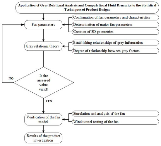
Figure 1. Framework of the development procedure.

For the evaluation of design parameters, it is usually difficult to predict the performance gain due to design optimization without making prototypes for measurement. However, the cost of making prototypes can be huge when the design optimization is based on a large number of design parameters. Therefore, simulation by CFD software is an important tool for a designer to predict the performance indicators of a new fan design, including air-flow rate and static pressure. By comparing these indicators, which are available from CFD simulation, the flow-field characteristics can be captured, and the optimal design can be determined among several candidates. The CFD simulation results are also compared with the experiment results in this study for the validation of this method.

2.2. Fan Model for Investigation

A schematic diagram of a symmetrical dual-impeller fan model in a case study is shown in Figure 2a, in which the initial impeller diameter is 80 mm. The main components, including the impellers, motors, and the base, are shown in Figure 2b, which is an exploded view of the fan model.

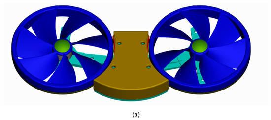
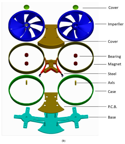
Figure 2. Fan parameters: (a) assembled dual-impeller fan; (b) exploded view of dual-impeller fan.

The operational principle of fans is mostly by means of the rotation of blades causing the pressure difference between the fore and aft ends to happen, driving the rapid flow of the surrounding air. This takes away the heat of the heat-dissipating body and results in a temperature decrease. For a typical design, after the design of a cooling element is shaped, the impedance curve of the element is fixed [13]. Therefore, it is the most often used approach in the typical cooling element design process to change the design of a fan to match the cooling element and enhance the overall cooling efficiency [14,15]. Therefore, it is rather important to find out and know the performance curves of different fans when designing cooling elements [16,17].

2.3. Fan Parameters Affecting the Performance Curve

• Blade pitch angle: The larger the pitch angle, the larger the pressure difference between the blade’s upper and lower surfaces. Under the same rotation speed, the air pressure is also larger with a larger pitch angle. However, when the pressure of the lower surface is too large, the phenomenon of recirculation may occur, and this instead reduces the fan’s performance. Therefore, the blade pitch angle should also be increased to a certain extent.
• Blade spacing: When the distance between the blades is too small, this leads to air-flow disturbance, which increases the friction on the blade surfaces and reduces fan efficiency. When the distance between blades is too large, this leads to an increase of pressure loss and insufficient air pressure [18].
• The number of blades: This affects other specifications of fan blades, such as the sectional curve and pitch angle. The width of each blade usually depends on its height. To guarantee that blade spacing will not affect the air pressure, the approach of increasing the number of blades is usually adopted as a remedy in comparatively thinner fans.

3. Research Methods

3.1. Gray Relational Theory

Assuming a space in relation to the gray information as

$$\left\{Q\left(X\right),R\right\}$$

(1)

where Q(X) is the factor set in relation to the gray information, and R is the relation of mutual influence. The factor subset X₀(k) is taken as the reference sequence, and X_i (k), i ≠ 0 is the comparison sequence [8]:

$$X_0=\left[x_0\left(1\right),x_0\left(2\right),\cdots ,x_i\left(k\right)\right]$$

(2)

$$X_i=\left[x_i\left(1\right),x_i\left(2\right),\cdots ,x_i\left(k\right)\right],i\in I,k\in N$$

(3)

The correlation coefficient in relation to the gray information for X_i(k) on X₀(k) is defined as

$$r_i\left(k\right)=r\left[X_0\left(k\right),X_i\left(k\right)\right]$$

(4)

The correlation degree in relation to the gray information for X_i on X₀ is

$$r\left(X_0,X_i\right)=\frac{1}{n}{\displaystyle \sum _{k=1}^{n}r\left[X_0\left(k\right),X_i\left(k\right)\right]}=\frac{1}{n}{\displaystyle \sum _{k=1}^n{r}_i\left(k\right)}$$

(5)

where the quantitative model of the correlation coefficient of gray information relationship for X_i(k) on X₀(k) is defined as

$$r_i\left(k\right)=r\left[X_0\left(k\right),X_i\left(k\right)\right]=\frac{\Delta \min +\zeta \Delta \max }{{\Delta }_{0,i}\left(k\right)+\zeta \Delta \max }$$

(6)

In the equation, ${\Delta }_{0,i}=\left|X_0\left(k\right)-X_i\left(k\right)\right|$ is the absolute difference of two comparison sequences, $\Delta \min =\underset{i\in I}{\min } \underset{k}{\min }\left|X_0\left(k\right)-X_i\left(k\right)\right|$ is the minimum of the absolute differences of all comparison sequences [19], $\Delta \max =\underset{i\in I}{\max } \underset{k}{\max }\left|X_0\left(k\right)-X_i\left(k\right)\right|$ is the maximum of the absolute differences of all comparison sequences, and $\zeta$ is the distinguishing coefficient. Its value is adjusted according to the practical demands of the system. Typically, its value is between 0 and 1, and is usually assigned as 0.5.

From the analysis mentioned above, four major equations of GRA and the quantitative model of the correlation degree are employed to establish the analysis model in relation to the gray information. The procedure is as follows.

Step 1: The initialization of the original sequence.

Step 2: Obtain the difference sequence, ${\Delta }_{0,i}=\left|X_0\left(k\right)-X_i\left(k\right)\right|$.

Step 3: Obtain the minimum of the absolute differences of all comparison sequences $\Delta \min$ and the maximum value $\Delta \max$.

Step 4: Calculate the gray correlation degree $r_i\left(k\right)$. The distinguishing coefficient is assigned as 0.5. Substitute the difference sequence, the minimum, and the maximum of the absolute differences into the quantitative model of the correlation degree in relation to the gray information to obtain the gray correlation degree $r_i\left(k\right)$.

Step 5: Calculate the correlation degree in relation to the gray information $X_i$ on $X_0$.

Step 6: Sort the degree of relationship between the major factor and all other factors in the gray system.

3.2. Governing Equations

In three-dimensional Cartesian coordinates, the governing equations are as follows (FLUENT User’s Guide) [1,20].

(1) Continuity equation:

$$\frac{\partial u}{\partial x}+\frac{\partial v}{\partial y}+\frac{\partial w}{\partial z}=0$$

(7)

(2) Momentum equations:

X direction:

$$\frac{\partial u}{\partial t}+\frac{\partial (u^2)}{\partial x}+\frac{\partial (uv)}{\partial y}+\frac{\partial (uw)}{\partial z}=-\frac{1}{\rho }\frac{\partial P}{\partial x}+v\left[\frac{{\partial }^{2}u}{\partial x^2}+\frac{{\partial }^{2}u}{\partial y^2}+\frac{{\partial }^{2}u}{\partial z^2}\right]$$

(8)

Y direction:

$$\frac{\partial v}{\partial t}+\frac{\partial (uv)}{\partial x}+\frac{\partial (v^2)}{\partial y}+\frac{\partial (vw)}{\partial z}=-\frac{1}{\rho }\frac{\partial (P-P_0)}{\partial z}+v\left[\frac{{\partial }^{2}v}{\partial x^2}+\frac{{\partial }^{2}v}{\partial y^2}+\frac{{\partial }^{2}v}{\partial z^2}\right]$$

(9)

Z direction:

$$\frac{\partial w}{\partial t}+\frac{\partial (uw)}{\partial x}+\frac{\partial (vw)}{\partial y}+\frac{\partial (w^2)}{\partial z}=-\frac{1}{\rho }\frac{\partial P}{\partial z}+v\left[\frac{{\partial }^{2}w}{\partial x^2}+\frac{{\partial }^{2}w}{\partial y^2}+\frac{{\partial }^{2}w}{\partial z^2}\right]$$

(10)

(3) Energy equation:

$$\frac{\partial T}{\partial t}+\frac{\partial (uT)}{\partial x}+\frac{\partial (vT)}{\partial y}+\frac{\partial (wT)}{\partial z}=\alpha (\frac{{\partial }^{2}T}{\partial x^2}+\frac{{\partial }^{2}T}{\partial y^2}+\frac{{\partial }^{2}T}{\partial z^2})+\frac{q}{p{C}_P}$$

(11)

(4) Governing equations can be represented by the general equations as follows:

$$\frac{\partial (\rho \phi )}{\partial t}+\frac{\partial (\rho \phi u)}{\partial x}+\frac{\partial (\rho \phi v)}{\partial y}+\frac{\partial (\rho \phi w)}{\partial z}=\frac{\partial }{\partial x}\left(\mathsf{\Gamma }\frac{\partial \phi }{\partial x}\right)+\frac{\partial }{\partial y}\left(\mathsf{\Gamma }\frac{\partial \phi }{\partial y}\right)+\frac{\partial }{\partial z}\left(\mathsf{\Gamma }\frac{\partial \phi }{\partial z}\right)+s$$

(12)

where $\frac{\partial (\rho \phi u)}{\partial x}+\frac{\partial (\rho \phi v)}{\partial y}+\frac{\partial (\rho \phi w)}{\partial z}$ is the convective term, $\frac{\partial }{\partial x}\left(\mathsf{\Gamma }\frac{\partial \phi }{\partial x}\right)+\frac{\partial }{\partial y}\left(\mathsf{\Gamma }\frac{\partial \phi }{\partial y}\right)+\frac{\partial }{\partial z}\left(\mathsf{\Gamma }\frac{\partial \phi }{\partial z}\right)$ is the diffusive term, S is the source term, and $\frac{\partial (\rho \phi )}{\partial t}$ is the unsteady term and is not considered when the system is in steady state. Symbol $\varnothing$ represents physical variables such as u, v, w, k, ε, and T (Table 1). The velocity components in the x, y, and z directions are u, v, and w, respectively; Γ is the corresponding diffusivity of each physical variable. Since we are looking for a steady-state solution, the variables are independent of time. Therefore, the partial derivatives of u, v, w, and T with respect to t are equal to zero.

Table 1. Symbols of independent variables.

Continuity	1
X-momentum	u
Y-momentum	v
Z-momentum	w

3.3. Standard k−ε Turbulence Model

Due to its extensive range of applications and reasonable precision, the standard k−ε model has become one of the main tools that are used for the calculation of turbulent flow fields. The standard k−ε turbulence model is a type of semi-empirical turbulence mode. Based on the fundamental physical control equations, the model can be used to derive the transport equations for the turbulence kinetic energy (k) and the rate of dissipation of turbulence energy (ε) as follows.

Turbulence kinetic energy equation (k)

$$\frac{\partial }{\partial t}(\rho k)+\frac{\partial }{\partial x_i}(\rho k{u}_i)=\frac{\partial }{\partial x_j}\left[\left(\mu +\frac{{\mu }_t}{{\sigma }_k^{}}\right)\frac{\partial k}{\partial x_j}\right]+G_k+G_b-\rho \epsilon -Y_M$$

(13)

(1) Equation of the rate of dissipation (ε)

$$\frac{\partial }{\partial t}(\rho \epsilon )+\frac{\partial }{\partial x_i}(\rho \epsilon u_i)=\frac{\partial }{\partial x_j}\left[\left(\mu +\frac{{\mu }_t}{{\sigma }_{\epsilon }^{}}\right)\frac{\partial \epsilon }{\partial x_j}\right]+C_{1s}\frac{\epsilon }{k}(G_k+C_{3\epsilon }{G}_b)-C_{2g\rho }\frac{{\epsilon }^2}{k}$$

(14)

(2) Coefficient of turbulent viscosity $\left({\mu }_t\right)$

$${\mu }_t=\rho C_{\mu }\frac{k^2}{\epsilon }$$

(15)

where $G_k$ indicates the turbulence kinetic energy that is generated by the laminar velocity gradient, $G_b$ indicates the turbulence kinetic energy that is generated by buoyancy, $Y_M$ indicates the fluctuation that is generated by the excessive diffusion in compressible turbulent flows, and ${\sigma }_k$ and ${\sigma }_{\epsilon }$ are the turbulence Prandtl number of kinetic energy and dissipation, respectively. Further, $C_{1\epsilon }$, $C_{2\epsilon }$, and $C_{3\epsilon }$ are empirical numbers, and their recommended numbers are shown in Table 2.

Table 2. Coefficients of standard k–ε turbulence model.

$C_{1\epsilon }$	$C_{2\epsilon }$	$C_u$	$C_k$	$C_{\epsilon }$
1.44	1.92	0.09	1.0	1.3

The k−ε model is based on the assumption that the flow field is fully turbulent and the molecular viscosity is negligible. Therefore, better results will be obtained from the calculation of fully turbulent flow fields.

3.4. Performance Testing Equipment for Wind Turbines

The main device of the performance testing equipment for fans is an outlet-chamber wind tunnel that conforms to AMCA 210-99. The principal parts include flow setting means, multiple nuzzles, flow-rate regulating devices, etc. The major function is to supply a good and stable flow field for measurement and acquire the complete performance curves [21].

3.5. Calculation of Flow Rates

Regarding the measured pressure difference between the nozzle outlet and inlet ($P{L}_5$ and $P{L}_6$), the flow rates on the cross-sections of nozzles shown in Figure 3 can be obtained by the nozzle coefficients. For the calculation of the outlet flow rate of the fan under test, the effect of density variations must be considered.

Figure 3. Schematic of measurement planes.

The equation for the calculation of flow rates in a test chamber with multiple nuzzles [22,23] is

$$Q_5=265.7Y\sqrt{\Delta P/{\rho }_5}{\displaystyle \sum _n\left(C_n{A}_{6n}\right)}$$

(16)

where

$Q_5$	the total flow rate measured by a bank of nozzles, CMM
$\Delta P$	the pressure difference across the nozzles, mm-Aq
${\rho }_5$	the air density upstream of the nozzles, $kg/m^3$
$Y$	expansion factor
$C_n$	the discharge coefficient of the nth nozzle (Nozzle Discharge Coefficient
$A_{6n}$	the cross-sectional area of the nth nozzle’s throat, $m^2$

3.6. Method of Measurements

(a) Start the measurement from the point of the maximum flow rate (i.e., the point at which the static pressure of a fan is zero). Pay attention to the pressure difference across the nozzles, which should be between 0.5 inch-Aq and 2.5 inch-Aq. If the differential pressure reading is not within this range, this indicates that the flow rate measured for the time being is incorrect. It is required to adjust the nozzle switch to respond to the variations in flow rate accordingly.

(b) After the completion of the data acquisition on the point of maximum flow rate, adjust the pressure to adequate values by means of the shutter of the auxiliary fan and inverter.

(c) Increase the pressure sequentially; the nozzle switch, the shutter of the auxiliary fan, and the inverter must be adjusted during each of the changes. After the system turns stable, then acquire a group of data by the data acquisition system [24,25].

(d) Store 10 sets of data in 10 different files, and use a computer program to calculate the values of air flow rate ($Q$), pressure ($\Delta P$), and efficiency ($\eta$).

(e) Import the calculation results into CAD software to draw the performance curves of the fans

This section expatiates on the procedures of the performance–curve measurement of fans based on the experience acquired after many rounds of measurements.

$$P_s=P_t-P_v$$

(17)

$$P_t=P_{t_2}-P_{t_1}$$

(18)

where P_s is the static pressure of the fan under test;

P_t is the total pressure of the fan under test;

P_v is the dynamic pressure of the fan under test;

$P_{t_2}$ is the total pressure at the fan’s outlet (or plane $P{L}_2$);

$P_{t_1}$ is the total pressure at the fan’s inlet (or plane $P{L}_1$).

Since in this experiment there was no duct at the inlet of the fan under test, therefore $P_{t_1}=0$ On the other hand, the measured static pressure at the outlet is the same as the static pressures measured at the measuring plane PL₇. Therefore, $P_{s_2}=P_{s_7}$.

$$P_{t_2}=P_{s_7}+P_v$$

(19)

$$P_s=P_{s_7}$$

(20)

It is concluded from the above equation that the static pressure of the fan under test happens to be equal to the static pressure obtained at the outlet test chamber $P_{t7}$. The calculation of dynamic pressures is

$$P_{v_2}=\frac{{\rho }_2{V}_2^2}{19.6}$$

(21)

where $P_{v_2}$ is the outlet dynamic pressure of the fan under test, mm-Aq;

$V_2$ is the outlet air velocity of the fan under test, m/s;

ρ₂ is the outlet air density of the fan under test, kg/m³;

and $V_2=\frac{Q_2}{60A_2}=\frac{Q}{60A_2}\cdot \frac{\rho }{{\rho }_2}$$=\frac{Q}{50{\rho }_2{A}_2}$

where Q₂ is the outlet flow rate of the fan under test, CMM;

Q is the standard flow rate of the fan under test, CMM;

A₂ is the outlet cross-sectional area of the fan under test, m²;

ρ is the density of air at STP (1.2 kg/m³).

$$P_t=P_s+P_v=P_s+P_{v_2}.$$

$$P_t=P_s+\frac{{\rho }_2{V}_2^2}{19.6}$$

(22)

3.7. Method of Measuring the Performance Curves of Fans

With a fixed amount of power, the flow rate varies inversely proportional to the output air pressure. Since the efficiency of fans changes as the flow rate varies, a non-linear relationship between the flow rate and the air pressure exists, and this forms the performance curve of fans [26]. The measurement process is shown in Figure 4.

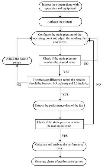
Figure 4. Operational flow chart of fan performance measurements.

3.8. Fan Performance Test Equipment

In terms of performance measurement, the detailed installation and operation of measurement equipment and instruments are described as follows. Regarding the fan performance measurement equipment, the fan performance test body used in this paper uses the AMCA 210-99 standard export wind tunnel, mainly including the main body. The main functions of the rectifier plate, multi-nozzle, and air volume adjustment device are to simulate the air flow conditions downstream of various fans, and to provide a good and stable measurement flow field, so that a complete performance curve can be obtained.

The test platform includes the body, rectifier plate, multiple nozzles, and auxiliary fans (see Figure 4, Figure 5, Figure 6, Figure 7, Figure 8 and Figure 9) to provide an ideal measurement benchmark; with the air volume adjustment device, it can simulate the outlet of the fan to be tested for various system impedances and even use in free air. The details are as follows:

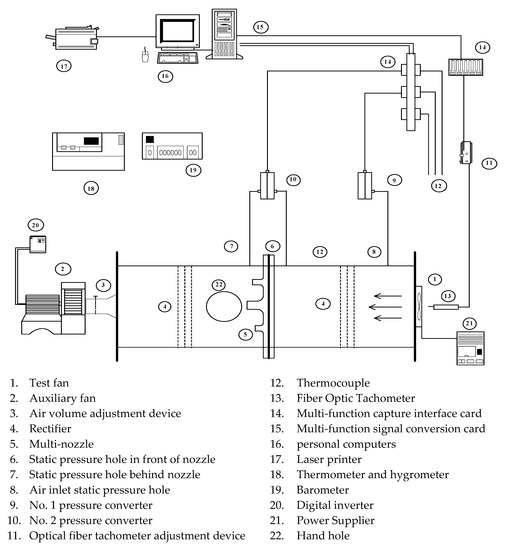
Figure 5. Main specifications of fan performance test.

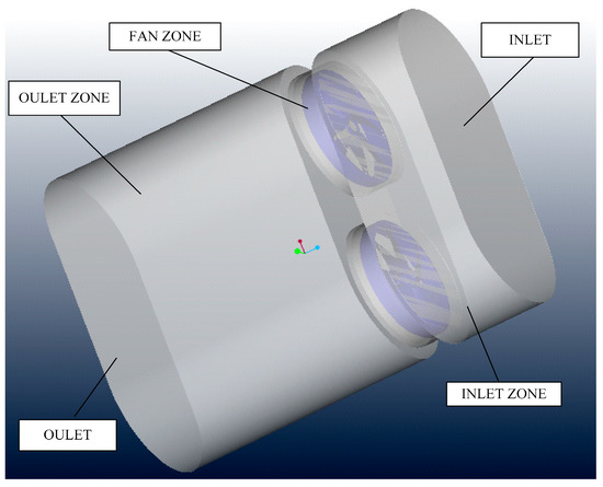
Figure 6. Model of the dual-impeller fan.

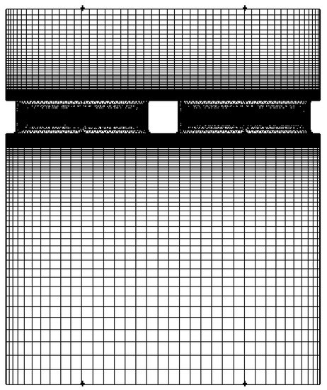
Figure 7. Structure of the numerical model of the dual-impeller fan for the case study.

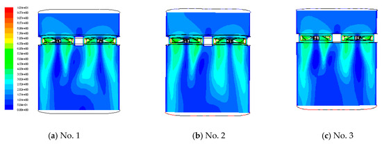
Figure 8. Contours of velocity on the centerline section.

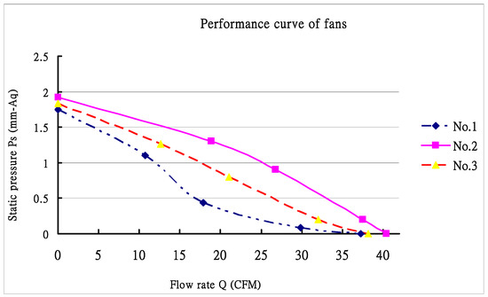
Figure 9. Fan performance curves.

(1) The body

The cross-sectional area of the outlet wind tunnel should be designed to be more than 16 times the maximum measurable area of the air outlet of the axial flow fan (because the test surface required by the axial flow fan is large, the wind tunnel is designed in this way).

(2) Rectifier

There is one set consisting of a front and one back box, with three pieces in each group. The area opening rate should be maintained at 50–60%. It is used to stabilize the fluid flow and ensure the reliability of measurement. Since the measurement of Sections 6 and 7 downstream of the nozzle and the static pressure of the fan are located upstream of the rectifier plate, in order to avoid the design of the rectifier plate affecting the measurement of these two sections, the maximum bounce velocity of the rectifier plate must be maintained at Sections 2 and 6 within 10% of the flow rate. Meanwhile, the measurement section (upstream of the nozzle) is also encountered downstream of the rectifier, so it specifies a local maximum speed of 0.1 M downstream of the rectifier unless the local maximum speed is less than 2 m/s; otherwise, it must not exceed 25% of the average flow rate.

(3) Multi-nozzle

This wind tunnel has seven nozzles with throat diameters of 30, 25, 25, 20, 15, 10, and 5. The nozzles with different diameters can measure different air volumes. The test fans with different nozzles can measure different air volumes. As air flows through the nozzle, a speed boundary layer is formed between the solid surface, and the correction factor is needed when calculating the flow rate. When the fluid velocity is slow, the speed boundary layer is relatively large, and the error is also relatively small when estimating the flow rate. It is large, so the Reynolds number will be set above 12,000 during the measurement; in order to avoid excessive changes in the air properties such as density and temperature, the flow rate will be controlled below Mach number 0.1 during the test. In order to prevent the flow fields between the nozzles from interfering with each other, the position of the nozzles is also clearly specified in the AMCA (Air Movement and Control Association, AMCA) specification, as shown in Figure 5.

4. Case Study

To investigate the influence of various parameters on fan performance, three different fan designs are investigated in this study and their parameters are shown in Table 3.

Table 3. Table of fan parameters.

Fan Design No.	No. 1	No. 2	No. 3
Rotation speed	2000	2000	2000
Leading-edge radius	61	63	65
Blade count	7	9	11
Outside diameter of the fan	70	72	74
Hub incidence angle	1	3	6
Tip incidence angle	0	3	6
Hub stagger angle	1	2	3
Tip stagger angle	0.75	0.85	0.95

The purpose of this step is to find new fan designs with potential performance gains, and those three representative designs as shown in Table 4 are categorized in order to determine the design direction of this study based on the results obtained from GRA.

Table 4. Models of new fan designs.

No. 1	No. 2	No. 3
7 blades	9 blades	11 blades

4.1. Analysis of the Correlation Degree of Gray Information

The procedures of building the analysis model in relation to the gray information are explained sequentially as follows.

Step 1: The initial values of the design parameters for evaluation are shown in Table 5. These values are converted by GRA for initialization, and the results are shown in Table 6.

Table 5. Initial values of design parameters.

Fan Design No.		1	2	3
Rotation speed	X0	2000	2000	2000
Leading-edge radius	X1	61	63	65
Blade count	X2	7	9	11
Outside diameter of the fan	X3	70	72	74
Hub incidence angle	X4	1	3	6
Tip incidence angle	X5	1	3	6
Hub stagger angle	X6	1	2	3
Tip stagger angle	X7	0.75	0.85	0.95

Table 6. Initialization of design parameters for gray relational analysis (GRA) $X_0=\left[x_0\left(1\right),x_0\left(2\right),\cdots ,x_i\left(k\right)\right]$.

Fan Design No.		1	2	3
Rotation speed	X0	0.3333	0.3333	0.3333
Leading-edge radius	X1	0.3228	0.3333	0.3439
Blade count	X2	0.2593	0.333	0.4074
Outside diameter of the fan	X3	0.3241	0.333	0.3426
Hub incidence angle	X4	0.1	0.3	0.6
Tip incidence angle	X5	0.1	0.3	0.6
Hub stagger angle	X6	0.1667	0.3333	0.5
Tip stagger angle	X7	0.2941	0.3333	0.3725

Step 2: Obtain the difference sequence,${\Delta }_{0,i}=\left|X_0\left(k\right)-X_i\left(k\right)\right|$, as shown in Table 7.

Table 7. Difference sequence ${\Delta }_{0,i}=\left|X_0\left(k\right)-X_i\left(k\right)\right|$.

Fan Design No.		1	2	3
Leading-edge radius	X1	0.0106	0.0000	0.0106
Blade count	X2	0.0741	0.0000	0.0741
Outside diameter of the fan	X3	0.0093	0.0000	0.0093
Hub incidence angle	X4	0.2333	0.0333	0.2667
Tip incidence angle	X5	0.2333	0.0333	0.2667
Hub stagger angle	X6	0.1667	0.0000	0.1667
Tip stagger angle	X7	0.0392	0.0000	0.0392

Step 3: From Table 7, the maximum and minimum values of the difference sequence can be determined as $\Delta \min ={\Delta }_{1,1}(2)=0.0000$ and $\Delta \max ={\Delta }_{4,3}\left(1\right)=0.2667$, respectively.

Step 4: Set the threshold value for gray correlation degrees at 0.5. The gray correlation degrees of various variance factors can be obtained as shown in Table 8.

Table 8. Gray correlation degree $r_i\left(k\right)$.

Fan Design No.		1	2	3
Leading-edge radius	X1	0.9265	1.0000	0.9265
Blade count	X2	0.6429	1.0000	0.6429
Outside diameter of the fan	X3	0.9351	1.0000	0.9351
Hub incidence angle	X4	0.3637	0.8000	0.3334
Tip incidence angle	X5	0.3637	0.8000	0.3334
Hub stagger angle	X6	0.4445	1.0000	0.4445
Tip stagger angle	X7	0.7727	1.0000	0.7727

Step 5: Calculate each variance factor $X_i$ for its average difference in the design parameters $X_0$ of the correlation degree in relation to the gray information $r\left(X_0,X_i\right)$. The resulting correlation degrees in relation to the gray information are shown in Table 9.

Table 9. Correlation degrees in relation to the gray information $r\left(X_0,X_i\right)$.

Factor		Correlation Degree
Leading-edge radius	X1	0.9510
Blade count	X2	0.7619
Outside diameter of the fan	X3	0.9567
Hub incidence angle	X4	0.4990
Tip incidence angle	X5	0.4990
Hub stagger angle	X6	0.6297
Tip stagger angle	X7	0.8485

4.2. Configuration of the Numerical Model

As shown in Figure 6, a numerical model of the dual-impeller fan was built for the case study. The dimensions of the inlet and outlet zones were determined based on the recommended values in order to reflect a real scenario of no impedance to the air flow into the ambient.

4.3. Settings of Model Parameters

A. Settings of boundary conditions

The main consideration of the settings of boundary conditions is to reflect the physical phenomena of the surrounding environment and objects around the target model. It is critical to meet the physical phenomena or else the calculation result of the simulation might be affected. A designer might also be misguided into making a wrong decision. In this case study, the boundary conditions include the inlet boundary condition, outlet boundary condition, and wall boundary condition, which are described as follows.

1. Inlet boundary condition: The inlet condition is for the initial calculation. In order to simulate the condition of a fan in an infinite domain, a normal atmospheric pressure of P0 is set at the inlet.

2. Outlet boundary condition: In order to simulation the air flow that is generated by the rotating impellers into the ambient, a normal atmospheric pressure of P0 is also set at the outlet.

3. Wall boundary condition: For a fluid flow passing along a wall, it needs to satisfy not only the non-permeable condition but also the no-slip condition.

In addition to the above-mentioned conditions, this case study includes the following assumptions in order to simplify the complexity of the flow field calculation.

• The flow field is at a steady state and the fluid is non-compressible air.
• The turbulence model that is used in this case study is k–ε with an eddy correction.
• The influence of gravitation is neglected.
• Relevant fluid properties, including the viscosity coefficient, density, and specific heat, are constants.
• A rotation speed of 2000 RPM is set for the fluid in the rotating zone.
• The fluid velocity at the surface of a solid is zero, and this is the no-slip condition.
• The heat radiation term and the buoyancy term are neglected, while physical properties are independent of temperature. This is because when the temperature of fluid is different at different locations, the buoyancy force is generated due to the variation in its density. However, air is driven by fans under forced convection while the natural convective effect is much less effective; therefore, the buoyance term can be neglected. On the other hand, the heat convective term due to the fluid’s sensible heat and latent heat is much larger than the heat radiation term, and therefore the radiation term can be neglected.

B. Mesh settings

As shown in Figure 7, the total number of cells is 1,957,013 for the dual impellers and 2,659,498 for the entire system, including the inlet and the outlet. As the mesh for the inlet and the outlet is used for the analysis of the upstream and downstream flow fields and for the boundary conditions, more cells are required at the locations that are closer to the dual impellers in order to simulate the complicated flow field locally. For the domain that is upstream to the dual impellers, the size of a cell is the largest at the inlet. Similarly, the size of a cell is the largest at the outlet for the domain that is downstream to the impellers. This is because no complex geometry exists at either the inlet or the outlet.

4.4. Simulation Results of Fans

The results of numerical simulation make it easy to understand the aerodynamic characteristics and the flow field of fans, which serve as the foundation for further investigation, analysis, and improvement. The contours of pressure, as shown in Figure 8, allow us to better understand the influence of pressure on the entire system in the flow field being analyzed as well as the velocity distribution of the fluid at the centerline section.

Lastly, the one to be compared is the resulting flow rate by numerical calculations. Based on the predicted flow rates of Table 10 by simulation at the outlet, it is known that the flow rate of 40.4 CFM in No. 2 is the maximum, whereas the change of incidence angle still has the effect of increasing the flow rate, but for the phenomenon of recirculation occurring along the upper edge of the impeller and between the blades, no big improvement is observed.

Table 10. Predicted flow rates by simulation.

Fan Design No.	1	2	3
Rotation speed when the maximum flow rate occurs (RPM)	2000	2000	2000
Maximum static pressure Ps (mm-Aq)	1.75	1.92	1.83
Maximum flow rate Q (CFM, Cubic feet per minute)	37.3	40.4	38.2

The weighted averages of the correlation degrees x₁~x_n are determined by the following equation. By applying the weighted averages to the flow rate and the static pressure of each fan design, the resulting values of maximum flow rate and maximum static pressure are shown in Table 11.

Table 11. Weighted averages of the maximum flow rate and the maximum static pressure.

Fan Design No.	1	2	3
Maximum static pressure Ps (mm-Aq)	0.3182	0.3491	0.3327
Maximum flow rate Q (CFM)	0.3218	0.3486	0.3296

In this study, simulation of three kinds of different fan designs designated as No. 1, No. 2, and No. 3 was conducted separately. Verifications of the various results obtained, including flow rates and air pressures, were also conducted by the simulation. With the simulation results obtained, consistency verification was further conducted on these results by the correlation degree of gray information. Observation and comparison were conducted both on the maximum static pressure and the maximum flow rate. It can be found in the simulation results that the maximum flow rate of No. 2 is apparently 9% higher than that of No. 1, whereas the maximum static pressure of No. 2 is also about 8% higher than that of No. 1, as shown in Figure 6.

4.5. Comparison Between the Results of Simulation and Experiment

Method of measuring the performance curve of a fan

The testing of fan characteristics is accomplished on a wind tunnel, as shown in Figure 9. The performance of a fan is usually determined by several operating points instead of a single point of static pressure versus air flow rate, because it is typically not considered as a stable system. Moreover, when a fan operates under a constant input power, the resulting flow rate varies inversely proportional to the output air pressure. In this study, the procedure of measuring fan performance is as follows.

• Preparatory work for measurements
  • Turn on the thermometer, hygrometer, barometer, fiber-optic tachometer, and inverter one hour before measurement. Make sure the equipment operates at a stable state. A testing workbench with a wind tunnel is shown in Figure 10a. The fan to be tested is mounted on the front plate of the main chamber. Care should be taken to ensure that the fan is sealed adequately to prevent leakage.
    

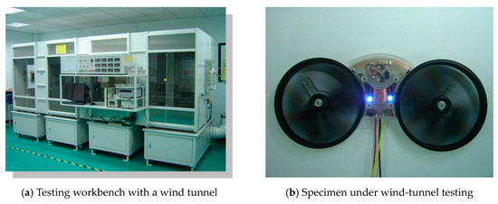    Figure 10. Wind-tunnel testing.
  • Turn on the test fan and the auxiliary blower for several minutes until both of them run stably. Adjust the blast gate from fully open to fully closed and check the air flow through the chamber. Check the readings of each of the equipment.
  • Measure the pressure difference between the free-flow condition (free deliver) and the no-flow condition (shut off). Divide the pressure difference into nine segments for determining the pressure increment and the data acquisition points.
• Measurement procedure
  • Start the measurement from the free-flow condition with a static pressure of 0. Pay attention to the pressure difference between the nozzle array. The pressure difference needs to be in the range of 0.5–2.5 mm-Aq or the measured air-flow rate could be incorrect. In this case, it is required to select another nozzle from the nozzle array for a different range of air-flow rates.
  • After the data under the free-flow condition are determined, use the blast gate and the inverter of the auxiliary blower to adjust the pressure to a desired range.
  • Increase the pressure to the next range of these nine segments by swapping the nozzle and adjusting the blast gate and the inverter. Use the data-acquisition system to take data of system readings after it has been stabilized. Repeat this step for all of these nine segments.
  • Pull out the data that are recorded in files and calculate the air-flow rate, air pressure, and efficiency of the computer program.
  • Summarize the calculation results in the performance curve of the fan.

The performance improvement that is predicted by the numerical simulation is further compared to the result that is obtained from the wind-tunnel testing, as shown in Table 12. Both the difference in the pressure drop and that in the air-flow rate are within 5%, which indicates a small difference between the simulation and the experiment results.

Table 12. Comparison between results from the simulation and the experiment.

	Results from the Simulation	Results from the Experiment
Rotation speed at the maximum flow rate (RPM)	2000
Maximum static pressure Ps (mm-Aq)	1.92	1.75
Maximum flow rate Q (CFM)	40.4	38.3

5. Results and Discussion

In this study, the gray design GRA was used to determine the important design parameters for improving the design performance of the fan with the best solution for symmetry or asymmetry. Based on the results obtained by GRA, the priority of design parameters for improving performance was determined, and GRA stated that the second design can provide better performance than the other two designs. The effects of these design parameters are further studied through numerical simulations and experiments. The simulation results also showed that the static pressure of the No. 2 design was 1.92 mm-Aq, and its flow rate was 40.4 CFM. Compared to the other two designs, it was obvious that performance-wise, No. 2 was the best of the three fan designs. By taking the weighted averages of the correlation degrees for the design parameters, the resulting maximum static pressures were No. 1: 0.3182, No. 2: 0.3491, and No. 3: 0.3327. Moreover, the maximum flow rates were No. 1: 0.3218, No. 2: 0.3486, and No. 3: 0.3296. It is clear that the maximum flow rate of No. 2 was the largest among these three designs. The most important design parameters can be determined by GRA at an earlier stage of fan design.

The results of the case study indicated that among fan parameters, the one with the greatest influence was the leading-edge radius. The outside diameter is another design parameter that shows a higher correlation degree. However, it is already known that an oversized fan could cause a stall, which leads to the phenomenon of rapidly deteriorating fan performance. Moreover, in space-constrained applications, the outside diameter is typically not selected as one of the design variables, because increasing the outside diameter leads to a bigger fan, which might fail to fit into the available space.

References

- Bredell, J.R.; KrÃÃger, D.G.; Thiart, G.D. Numerical investigation of fan performance in a forced draft air-cooled steam condenser. Appl. Therm. Eng. 2006, 26, 846–852. [Google Scholar] [CrossRef]
- Hurault, J.; Kouidri, S.; Bakir, F.; Rey, R. Experimental and numerical study of the sweep effect on three-dimensional flow downstream of axial flow fans. Flow Meas. Instrum. 2010, 21, 155–165. [Google Scholar] [CrossRef]
- Rhee, D.H.; Cho, H.H. Effect of vane/blade relative position on heat transfer characteristics in a stationary turbine blade: Part 2. Blade surface. Int. J. Therm. Sci. 2008, 47, 1544–1554. [Google Scholar] [CrossRef]
- Lai, H.H.; Chen, C.H.; Chen, Y.C.; Yeh, J.W.; Lai, C.F. Product design evaluation model of child car seat using gray relational analysis. Adv. Eng. Inform. 2009, 23, 165–173. [Google Scholar] [CrossRef]
- Wei, G.W. Grey relational analysis method for 2-tuple linguistic multiple attribute group decision making with incomplete weight information. Expert Syst. Appl. 2011, 38, 4824–4828. [Google Scholar] [CrossRef]
- Qiu, B.; Wang, F.; Li, Y.; Zuo, W. Research on Method of Simulation Model Validation Based on Improved Grey Relational Analysis. Phys. Procedia 2012, 25, 1118–1125. [Google Scholar] [CrossRef]
- Li, Q.X. Grey dynamic input–output analysis. J. Math. Anal. Appl. 2009, 359, 514–526. [Google Scholar] [CrossRef][Green Version]
- Trivedi, H.V.; Singh, J.K. Application of Grey System Theory in the Development of a Runoff Prediction Model. Biosyst. Eng. 2005, 92, 521–526. [Google Scholar] [CrossRef]
- Li, L.; Huang, G.; Chen, J. Aerodynamic characteristics of a tip-jet fan with a large blade pitch angle. Aerosp. Sci. Technol. 2019, 91, 49–58. [Google Scholar] [CrossRef]
- Wang, Z.; Wu, Y.; Lu, S.; Meng, X.; Zhang, J. A study on model experiment and aerodynamic match of Wind Energy Fan. Sustain. Cities Soc. 2019, 49, 101618. [Google Scholar] [CrossRef]
- Wu, Y.; Pan, D.; Peng, Z.; Hua, O. Blade force model for calculating the axial noise of fans with unevenly spaced blades. Appl. Acoust. 2019, 146, 429–436. [Google Scholar] [CrossRef]
- Villiers, D.J.; Mathews, M.J.; Maré, P.; Kleingeld, M.; Arndt, D. Evaluating the impact of auxiliary fan practices on localised subsurface ventilation. Int. J. Min. Sci. Technol. 2019, 29, 933–941. [Google Scholar] [CrossRef]
- Tournier, J.M.; El-Genk, M.S. Axial flow, multi-stage turbine and compressor models. Energy Convers. Manag. 2009, 51, 16–29. [Google Scholar] [CrossRef]
- Qian, X.; Deba, D. Design of heterogeneous turbine blade. Comput. Aided Des. 2003, 35, 319–329. [Google Scholar] [CrossRef]
- Lin, H.H. Application of Fuzzy Decision Model to the Design of a Pillbox for Medical Treatment of Chronic Diseases. Appl. Sci. 2019, 9, 4909. [Google Scholar] [CrossRef]
- Lin, S.C.; Huang, C.L. An integrated experimental and numerical study of forward–curved centrifugal fan. Exp. Therm. Fluid Sci. 2002, 26, 421–434. [Google Scholar] [CrossRef]
- Li, Y.L.; Liu, J.; Ou, H.; Du, Z.H. Internal flow mechanism and experimental research of low pressure axial fan with forward-skewed blades. J. Hydrodyn. Ser. B 2008, 20, 299–305. [Google Scholar] [CrossRef]
- Niu, M.; Zang, S. Experimental and numerical investigations of tip injection on tip clearance flow in an axial turbine cascade. Exp. Therm. Fluid Sci. 2011, 35, 1214–1222. [Google Scholar] [CrossRef]
- Yao, C. Application of Gray Relational Analysis Method in Comprehensive Evaluation on the Customer Satisfaction of Automobile 4S Enterprises. Phys. Procedia 2012, 33, 1184–1189. [Google Scholar]
- FLUENT User’s Guide. Available online: https://www.ansys.com/products/fluids/ansys-fluent (accessed on 1 January 2019).
- Lin, H.H.; Huang, Y.Y. Application of ergonomics to the design of suction fans. In Proceedings of the 1st IEEE International Conference on Knowledge Innovation and Invention, Jeju Island, South Korea, 23–27 July 2018; pp. 203–206. [Google Scholar]
- Hsiao, S.W.; Lin, H.H.; Lo, C.H.; Ko, Y.C. Automobile shape formation and simulation by a computer-aided systematic method. Concurr. Eng. Res. Appl. 2016, 24, 290–301. [Google Scholar] [CrossRef]
- Lin, H.H. Improvement of Human Thermal Comfort by Optimizing the Airflow Induced by a Ceiling Fan. Sustainability 2019, 11, 3370. [Google Scholar] [CrossRef]
- Lin, H.H.; Hsiao, S.W. A Study of the Evaluation of Products by Industrial Design Students. Eurasia J. Math. Sci. Technol. Educ. 2018, 14, 239–254. [Google Scholar] [CrossRef]
- Hsiao, S.W.; Lin, H.H.; Lo, C.H. A study of thermal comfort enhancement by the optimization of airflow induced by a ceiling fan. J. Interdiscip. Math. 2016, 19, 859–891. [Google Scholar] [CrossRef]
- Lin, H.H.; Cheng, J.H. Application of the Symmetric Model to the Design Optimization of Fan Outlet Grills. Symmetry 2019, 11, 959. [Google Scholar] [CrossRef]
© 2020 by the authors. Licensee MDPI, Basel, Switzerland. This article is an open access article distributed under the terms and conditions of the Creative Commons Attribution (CC BY) license (http://creativecommons.org/licenses/by/4.0/).