A Remote Sensing Baseline and Time Sequence of Land Cover Change for the Conservation of Rainbowfish (Melanotaenia spp.) from the Bird’s Head Peninsula, Western New Guinea

Margaret Kalacska; Oliver Lucanus; Hans Georg Evers; Juan Pablo Arroyo-Mora

doi:10.3390/land15020332

Abstract

Rainbowfish of the genus Melanotaenia are highly endemic freshwater fishes found only in Australia and New Guinea. Although widespread, most species have narrow geographic ranges, making them particularly vulnerable to environmental change. Currently, 43 described (and many undescribed) Melanotaenia species occur in the Bird’s Head and Bird’s Neck region of Western New Guinea, 29 of which are currently classified as critically endangered, endangered, or vulnerable by the IUCN Red List, including two that may be extinct in the wild. We generated a high-spatial-resolution baseline land cover classification of rainbowfish habitats using low-cloud Planet Labs quarterly basemap mosaics and compared it with a moderate-resolution Landsat 8 OLI-derived classification to assess how spatial resolution influences land cover classification. Using the full 40-year Landsat archive, we quantified decadal land cover change around species type localities and identified localized disturbance events that may affect rainbowfish habitats. For species described from large rivers and lakes, changes in water-body extent over time were quantified. Deforestation varied widely, ranging from little or no detectable change in remote, difficult-to-access locations (e.g., M. misoolensis, M. sneideri), to landscapes heavily modified by logging, urbanization, mining, and agriculture (e.g., M. boesemani, M. arfakensis). Around the type localities, from the high-resolution imagery, we detected ~2939 ha of cleared land, whereas from the Landsat classification we identified only 31 ha of clearing, indicating that most of the fine-scale deforestation was not resolved at the Landsat scale. Time-sequence analyses indicate that over one-third of type localities experienced one or more localized disturbance events over the last 40 years. Land cover change in this region is highly dynamic and differs from commonly studied frontier deforestation patterns elsewhere. It also underscores a critical conservation challenge where rainbowfish species are being discovered in landscapes that are simultaneously undergoing rapid, spatially heterogeneous change. The same infrastructure that enables biological exploration also accelerates habitat modification. These changes threaten the persistence of highly endemic rainbowfish and underscore the value of multi-scale spatial and temporal remote sensing approaches for assessing habitat change in remote, biodiverse regions. The framework presented here is also broadly applicable to other narrowly distributed endemic taxa.

Keywords:

CubeSat; land cover; land use; biodiversity; satellite; forest cover; freshwater; Landsat; GEOBIA

1. Introduction

Though often overshadowed by large-scale industrial logging and land conversion for agriculture and other land uses, small-scale deforestation (e.g., [1]) can have substantial ecological impacts, especially for endemic species. The removal of even small forest areas (e.g., 1–100 hectares) can disrupt fragile ecosystems such as freshwater habitats [2], which support local endemic fish species highly adapted to narrow environmental conditions (e.g., temperature, water chemistry, clarity, and food availability). Even minor alterations can lead to habitat fragmentation, reduced genetic diversity, and the extinction of vulnerable species [3]. Forest cover loss at both local and landscape scales can further disrupt soil health and hydrological processes, because trees play a critical role in maintaining soil structure and reducing erosion [4,5]. When trees or forest stands are removed, soils become more susceptible to degradation, increased runoff, and sedimentation into nearby water bodies, which can degrade water quality and affect the aquatic biota [6,7]. Moreover, ref. [8] shows that forest cover loss alters hydrologic and climatic conditions across forest biomes, with tropical rainforests exhibiting early-stage declines in water yield and concurrent warming following relatively small reductions in tree cover. Thus, understanding the effects of small-scale deforestation across spatial scales is critical for prioritizing conservation efforts for endemic species in freshwater ecosystems.

Melanotaeniids (order Atheriniformes) are one of only four endemic fish families (alongside Lepidogalaxidae, Neoceradontidae, and Pseudomugilidae) with a distribution restricted to the freshwaters of Australia–New Guinea. The Melanotaeniidae or rainbowfishes are small (10–12 cm SL), colorful fishes that occur in a wide range of lotic and lentic habitats from clear, rapidly flowing streams to semi-stagnant mudholes. While many species have quite narrow ranges, they are the most widespread family within Australia and New Guinea, where they are often the most abundant fish present [9]. The highest species diversity occurs in New Guinea, which can be divided into three major biogeographic regions. North of the Central Range, species diversity is dominated by the genera Chilatherina, Glossolepis, and Melanotaenia. South of the Central Range, Iriatherina and a particularly high diversity of Melanotaenia species can be found. The third region comprises the Vogelkop Peninsula (Bird’s Head Peninsula) together with the region to the southeast, commonly referred to as the Bird’s Neck. Recent phylogenetic evidence indicates that Melanotaenia contains three main lineages, northern, southern, and western, corresponding with these major biogeographic regions [9]. Within the western region, 29 species of Melanotaenia are classified as critically endangered, endangered, or vulnerable by the IUCN Red List, including two that may be extinct in the wild.

Satellite time-sequence analysis of land cover and land use change (e.g., forest vs. non-forest) is a crucial approach for understanding how landscapes evolve over time due to both natural dynamics (e.g., wildfires, forest gaps) and human activities (e.g., deforestation, urban development) [10,11]. Long-term archived satellite imagery provides consistent, repeatable, and broad-scale observations of the Earth’s surface, making it an invaluable tool for monitoring land cover change across different temporal (years to decades) and spatial scales (local to landscape). The Landsat series’ extensive archives, spanning over 50 years of digital, multispectral (four to seven spectral bands) imagery at medium spatial resolution (30 m), are the most widely used Earth observation (EO) dataset for satellite image time-series analysis [12]. This wealth of EO data from Landsat provides consistent surface reflectance suitable for applying diverse time-series methods and has been widely used worldwide across different applications and geographic locations [13]. Given the medium spatial resolution from Landsat, applications involving features below a small minimum mapping unit [14], or those requiring very high temporal resolution (e.g., to overcome persistent cloud cover in tropical regions), can benefit from newer commercial EO systems such as the Planet Dove constellation, which provides satellite imagery dating back to 2016 with near-daily revisit times at a spatial resolution of ~4 m [15].

In this study, we assess land cover change surrounding the type localities of 43 rainbowfish species endemic to the Bird’s Head and Bird’s Neck region of Western New Guinea, within 5 km and 300 m spatial buffers. Previous remote sensing studies have mapped land cover and forest change broadly across Western New Guinea (e.g., [16,17,18,19,20,21]); however, these analyses have not been explicitly designed to evaluate habitat change at spatial scales relevant to narrowly distributed freshwater taxa. Forest loss in the region is primarily associated with timber extraction, oil palm expansion, and agriculture [19]. Due to persistently high cloud cover [22], we first generated a baseline high spatial resolution land cover classification using a low-cloud Planet Labs quarterly basemap mosaic and compared it to a classification derived from moderate resolution Landsat 8 OLI imagery to evaluate how spatial resolution influences the detection of change. We then used the full 40-year Landsat archive to produce three decadal change analyses (within 5 km buffers) and to identify localized disturbance events within 300 m buffers that may affect rainbowfish habitat conditions (e.g., via altered thermal regimes). For species inhabiting large rivers and lakes, where small-area buffers are less informative, we instead quantified changes in waterbody extent. Our study underscores the importance of multi-scale spatial and temporal analyses in this understudied yet highly biodiverse region [23]. The approaches presented here are broadly applicable and could be used to assess habitat change for other narrowly distributed endemic plant and animal taxa.

2. Materials and Methods

2.1. Study Area

New Guinea is the world’s largest tropical island and the most floristically diverse island globally [23]. It ranks among the top 1% of global regions for conservation importance based on terrestrial biodiversity, carbon storage, and freshwater resources [24]. Politically, the island is divided between the independent nation of Papua New Guinea in the east and the western half administered by Indonesia. The western region, referred to as Western New Guinea, Indonesian New Guinea, or Tanah Papua, is administratively divided into the provinces of Papua and West Papua. In this study, we focus on the Bird’s Head Peninsula (Vogelkop) and the adjacent Bird’s Neck region of Western New Guinea (Figure 1). We also include the four islands closest to the mainland with described rainbowfish species (Rumberpon, Misool, Batanta, and Waigeo), resulting in a total study area of 119,262.6 km².

Figure 1. Map of the study area in Western New Guinea (Bird’s Head and Bird’s Neck). The names of the described species (red points) included in the analyses can be found in Table 1. The yellow points are examples of currently undescribed, potentially new species found on an expedition by author H.G.E. The blue points also represent potentially new species (J. Graf pers. communication, 15 January 2026). The yellow dashed line indicates the Central Ayamaru Plateau.

Table 1. List of Melanotaenia species included in this study. Map No. corresponds to locations shown in Figure 1. The IUCN Red List categories are CR = critically endangered, EN = endangered, LC = least concern, NA = not assessed, NT = near threatened, PE = possibly extinct in the wild, VU = vulnerable. YC is the year the species holotype was collected, as mentioned in the description.

Species	YC	Map No.	IUCN Red List	IUCN Threats
M. ajamaruensis (Allen & Cross, 1980)	1955	14	CR-PE	-Invasive non-native/alien species/diseases
M. ammeri (Allen, Unmack & Hadiaty, 2008)	2008	29	NT	-Oil & gas drilling
M. angfa (Allen, 1990)	1989	25	LC
M. arfakensis (Allen, 1990)	1989	19	EN	-Housing & urban areas -Annual & perennial non-timber crops -Mining & quarrying -Invasive non-native/alien species/diseases
M. arguni (Kadarusman, Hadiaty & Pouyaud, 2012)	2010	28	EN	-Annual & perennial non-timber crops -Oil & gas drilling
M. batanta (Allen & Renyaan, 1998)	1998	3	VU	-Habitat shifting & alteration
M. boesemani (Allen & Cross, 1980)	1948	15	EN	-Fishing & harvesting aquatic resources -Invasive non-native/alien species/diseases -Problematic native species/diseases -Habitat shifting & alteration
M. bowmani (Allen, Unmack & Hadiaty, 2016)	2012	43	CR	-Mining & quarrying
M. catherinae (de Beaufort, 1910)	1910	1	LC	-Mining & quarrying -Invasive non-native/alien species/diseases
M. dumasi (Weber, 1907)	1903	41	LC
M. erikrobertsi (Allen, Hadiaty & Unmack, 2014)	1982	8	LC
M. etnaensis (Allen, Unmack & Hadiaty, 2016)	2013	39	LC
M. fasinensis (Kadarusman, Sudarto, Paradis & Pouyaud, 2010)	2007	12	EN	-Wood & pulp plantations -Marine & freshwater aquaculture -Invasive non-native/alien species/diseases
M. flavipinnis (Allen, Hadiaty & Unmack, 2014)	1999	6	LC
M fredericki (Fowler, 1939)	1938	7	NT	-Housing & urban areas -Commercial & industrial areas -Annual & perennial non-timber crops -Fishing & harvesting aquatic resources
M. grunwaldi (Allen, Unmack & Hadiaty, 2016)	2012	42	VU	-Mining & quarrying
M. irianjaya (Allen, 1985)	1982	44	VU	-Annual & perennial non-timber crops -Oil & gas drilling -Logging & wood harvesting
M. cf irianjaya	2013 *	17	VU	-Annual & perennial non-timber crops -Oil & gas drilling -Logging & wood harvesting
M. jakora (Graf, Ohee, Herder & Haryono, 2023)	2006	20	NA
M. kamaka (Allen & Renyaan, 1996)	1991	37	LC
M. klasionensis (Kadarusman, Avarre & Pouyaud, 2015)	2008	10	CR	-Annual & perennial non-timber crops -Invasive non-native/alien species/diseases
M. kokasensis (Allen, Unmack & Hadiaty, 2008)	2008	26	CR	-Housing & urban areas -Logging & wood harvesting
M. lacunosa (Allen, Unmack & Hadiaty, 2016)	1997	38	CR	-Problematic native species/diseases -Droughts
M. lakamora (Allen & Renyaan, 1996)	1995	35	EN	-Habitat shifting & alteration
M. laticlavia (Allen, Hadiaty & Unmack, 2014)	2013	18	VU	-Mining & quarrying
M. longispina (Kadarusman, Avarre & Pouyaud, 2015)	2008	9	CR	-Annual & perennial non-timber crops -Invasive non-native/alien species/diseases
M. mairasi (Allen & Hadiaty, 2011)	2010	33	CR	-Droughts
M. mamahensis (Allen, Unmack & Hadiaty, 2016)	2015	40	VU	-Invasive non-native/alien species/diseases
M. manibuii (Kadarusman, Slembrouck & Pouyaud, 2015)	2007	21	EN	-Housing & urban areas -Annual & perennial non-timber crops -Mining & quarrying -Invasive non-native/alien species/diseases
M. misoolensis (Allen, 1982)	1948	5	LC
M. multiradiata (Allen, Hadiaty & Unmack, 2014)	1999	16	VU	-Housing & urban areas -Invasive non-native/alien species/diseases
M. naramasae (Kadarusman, Nugraha & Pouyaud, 2015)	2009	27	EN	-Annual & perennial non-timber crops -Mining & quarrying -Logging & wood harvesting
M. parva (Allen, 1990)	1989	24	CR-PE	-Invasive non-native/alien species/diseases
M. pierucciae (Allen & Renyaan, 1996)	1995	36	LC
M. rumberponensis (Kadarusman, Ogistira & Pouyaud, 2015)	2008	23	LC
M. salawati (Kadarusman, Sudarto, Slembrouck & Pouyaud, 2011)	2008	4	NT	-Habitat shifting & alteration
M. sembrae (Kadarusman, Avarre & Pouyaud, 2015)	2008	13	EN	-Housing & urban areas
M. sikuensis (Kadarusman, Sudarto & Pouyaud, 2015)	2007	22	VU	-Mining & quarrying
M. sneideri (Allen & Hadiaty, 2013)	2013	34	CR	-Droughts
M. susii (Kadarusman, Avarre & Pouyaud, 2015)	2008	11	CR	-Housing & urban areas -Logging & wood harvesting -Invasive non-native/alien species/diseases
M. synergos (Allen & Unmack, 2008)	1992	2	VU	-Habitat shifting & alteration
M. urisa (Kadarusman, Setiawibawa & Pouyaud, 2012)	2010	30	CR	-Logging & wood harvesting -Habitat shifting & alteration
M. veoliae (Kadarusman, Caruso & Pouyaud, 2012)	2010	31	VU	-Logging & wood harvesting -Droughts
M. wanoma (Kadarusman, Segura & Pouyaud, 2012)	2010	32	VU	-Logging & wood harvesting -Droughts

* The year author H.G.E. collected specimens.

The Bird’s Head Peninsula exhibits pronounced geographic and topographic heterogeneity. In the north, the Tamrau Mountains in the northwest and the Arfak Mountains in the northeast dominate the landscape, separated by the broad Kebar Valley (Figure 1). The Central Ayamaru Plateau and the Bomberai Peninsula are characterized by extensive karst landscapes. The Bomberai Peninsula remains largely undeveloped, with vast tracts accessible only by air. By contrast, the Central Ayamaru Plateau, including the Ayamaru Lakes, smaller adjacent lacustrine systems, and the southern corridor from Sorong to Teminabuan, has undergone rapid urban expansion over recent decades.

Karst formations on the Central Ayamaru Plateau are particularly difficult to traverse and host complex hydrological systems in which streams and rivers flow at the surface for several kilometers before disappearing underground, only to re-emerge farther downstream. For example, Melanotaenia fasinensis is known exclusively from the Fasin River, a short reach of the Kladuk River system near Ween village that becomes subterranean after only a few kilometers [25]. Melanotaenia species inhabit almost every creek and river on the Central Ayamaru Plateau.

The Bird’s Neck region is dominated by the Lengguru Foldbelt, a complex orogenic system formed through oblique convergence between the Australian and Pacific plates [26]. The region comprises a series of imbricated, fault-bounded mountain wedges that isolate numerous endorheic and semi-endorheic intermontane valleys. In the lower reaches of these valleys, extensive karst landscapes have developed, forming complex subterranean systems characterized by deeply incised canyon networks, caves, and fragmented surface–subsurface river systems. This geomorphic complexity underpins exceptionally high biodiversity, with numerous new plant and animal taxa described from the region in recent years (e.g., [27,28]). Notably, of the 15 rainbowfish species documented during a large multinational expedition in 2014, more than half are considered likely to be new to science [29].

Despite this biological significance, large portions of the region, including near Bintuni Bay, remain isolated. Exceptionally rugged karst terrain occurs in the Lengguru Foldbelt, the Bomberai Peninsula, and within the adjacent Triton Lakes complex (Lake Kamakawaiar, Lake Lakamora, and Lake Aiwasso), where access is limited to helicopter transport under favorable weather conditions. These logistical constraints have made field exploration both challenging and costly, contributing to persistent knowledge gaps in one of the island’s most biodiverse landscapes. The karst landscapes of the region are widely recognized as among the most inaccessible and understudied ecosystems [30].

The complex geologic history of Western New Guinea, particularly within the Bird’s Head and Bird’s Neck regions, has generated exceptional habitat diversity and high species richness [31]. Numerous small, isolated river basins drain rapidly from mountainous and karst terrain directly to the sea. This geomorphological and hydrological isolation has promoted narrowly restricted species distributions and exceptionally high levels of endemism, particularly among freshwater taxa.

2.2. The Family Melanotaeniidae

Within Western New Guinea (Bird’s Head and Bird’s Neck), there is a complex of Melanotaenia species with similar morphology and coloration. A number of these species occur in the region near Lake Ayamaru, e.g., Melanotaenia ajamaruensis, M. boesemani, M. ericrobertsi, M. fasinensis, M. longispina, M. susii and M. klasionensis (referred to as the species from Central Ayamaru Plateau according to [32]) Others, such as M. arfakensis, M. irianjaya, M. veoliae, M. laticlavia, M. multiradiata, and M. wanoma, occur more broadly across the Birds Head region. Several species are endemic to the isthmus between the Birds Head and the Birds Neck, such as M. angfa, M. parva, M. sikuensis, M. manibuii, and others. Finally, there is a group of species endemic to the Bird’s Neck, namely three species of the “Goldiei group” that apparently migrated from the South (M. goldiei and related species typically occurr in the South of New Guinea with their “sister” species complex, the “Trifasciata group” from Northern Australia) through the Omba–Woromi corridor, a low elevation (up to 160 m) area linking the respective southern and northern drainages [33] along with their close southern relatives: M. bowmani, M. etnaensis, M. dumasi, M. grunwaldi, M. lacunosa and M. mamahensis. The Bird’s Head region and the adjacent Bird’s Neck of West Papua are hot spots for recent discoveries. A summary provided by ref. [34] included the seven species known to inhabit the Bird’s Head mainland at that time. Using DNA barcoding, ref. [30] found exceptionally high levels of cryptic diversity and endemism in the Bird’s Head and Bird’s Neck regions. Their analyses revealed nearly 30 distinct evolutionary lineages within the 15 nominal rainbowfish species sampled, with all detected lineages restricted to a single lake or watershed. Currently, 37 described species, plus several undescribed forms, are known from the region. In this study, we include the 37 described species as well as six species from the nearby islands of Rumberpon, Waigeo, Salawati, Batanta, and Misool (Figure 1, Table 1) for a total of 43 species. For M. irianjaya (Figure 1, map #44), a species widespread north and south of Bintuni Bay [35], we also include a second sampling location (M. cf. irianjaya; Figure 1, map #17) based on specimens collected by author H.G.E. in 2013. Several rainbowfish species are widely represented in the aquarium hobby [30], with examples of four commonly traded species shown in Figure 2.

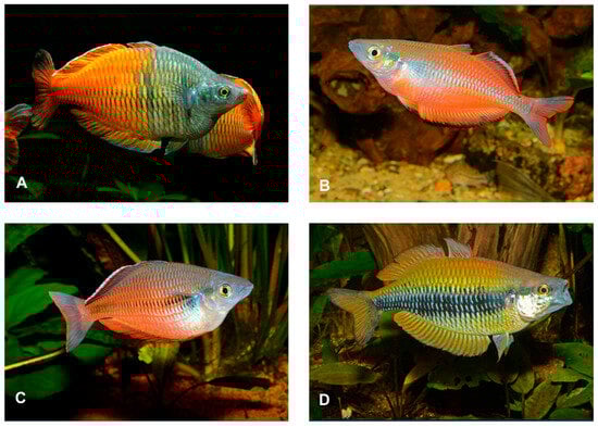
Figure 2. Aquarium photographs of male specimens of (A) M. boesemani, (B) M. susii, (C) M. fasinensis, and (D) M. sikuensis.

The collection and formal description of Melanotaenia species were sporadic throughout the 20th century, with low numbers recorded per year (Figure 3). Activity increased from the 1990s onward, culminating in a pronounced surge between 2008 and 2015. Species descriptions are strongly clustered between 2010 and 2016, reflecting a concentrated period of taxonomic activity. Overall, most formal descriptions are relatively recent, highlighting that a large proportion of known rainbowfish diversity has only been documented in the past two decades. In addition to the relatively high number of described Melanotaeniids, there are still many undescribed forms. Dense vegetation and challenging terrain with limited access in much of Western New Guinea make it almost impossible to investigate the distribution pattern for these species, and the genetic relationships between the different forms are only partially known [32]. Photographs illustrating some examples of Melanotaenia habitats are shown in Figure 4.

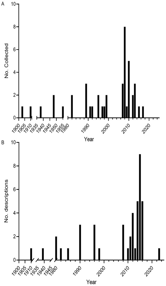
Figure 3. (A) Number of Melanotaenia type specimens from the study area collected per year; (B) number of Melanotaenia species described per year.

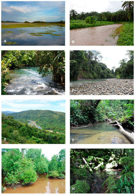
Figure 4. Examples of rainbow fish habitats in the study area: (A) Lake Ayamaru, home to M. boesemani. (B) Prafi River near Manokwari, type locality of M. arfakensis. (C) The Kali Alawit creek in the Central Ayamaru Plateau, habitat of M. ajamaruensis. (D) Braidplain of the Sungai Mega stream in the Tamrau Mountains, habitat of M. ericrobertsi. (E) Primary forest is still commonly found surrounding rivers on the Bird’s Head Peninsula. (F) The Kali Aitafoh in the Ayamaru District drains the foothills of the Tamrau mountains. (G) Mangroves north of Sorong. (H) Many creeks and rivers on the Central Ayamaru Plateau are spring water, flowing over ground for just a few kilometers before going underground again. The soft limestone of this karst region covers a labyrinth of caves and underground waterways.

2.3. Satellite Imagery

We used several satellite data sources, including the complete Landsat 4–9 archive from 1984 to 2025, a global quarterly cloud-minimized basemap from Planet Labs, and high-resolution multispectral imagery from the PlanetScope Dove-R, SuperDove, and RapidEye constellations. Each source, which corresponds to a different scale of ecological threat, is described here briefly.

2.3.1. Imagery Description

The Landsat program is the longest continuous satellite record of the Earth’s land surface, beginning with Landsat-1 in 1972 and continuing through Landsat-9 launched in 2021, with Landsat Next planned for launch in late 2030/31 [36]. The series consists of successive multispectral missions providing medium-resolution (30 m pixel size) global imaging. Landsat-4 TM, operational 1982–1993, and Landsat-5 TM, operational 1984–2013, provided seven spectral bands spanning the visible to shortwave infrared wavelengths plus one thermal band. Landsat-7 ETM+ (1999–2025) also provided the seven spectral bands, one thermal band, and an additional 15 m panchromatic band. The newest in the series, Landsat-8 and Landsat-9 OLI/TIRS launched in 2013 and 2021, respectively, expanded the system to 11 operational bands (eight reflective, one panchromatic, plus two thermal). For all analyses, only the reflective optical bands with a 30 m pixel size were used. The Landsat series has been comprehensively described in the literature, including sensor development and long-term data continuity [37,38]. These data were used for a moderate-resolution land cover map generation, multi-decadal forest cover change analyses, a time-sequence analysis of disturbance, and to supplement the surface water extent analysis (Section 2.4.2, Section 2.4.4, Section 2.5 and Section 2.6).

The global quarterly cloud-minimized basemap is a mosaic constructed from best-available daily PlanetScope imagery using automated cloud and haze masking and is optimized for human viewing and computer vision analytics [39]. It was used to create the high-spatial resolution baseline land cover classification (Section 2.4.1). The PlanetScope constellation consists of more than 430 triple-CubeSats (i.e., miniature satellites). The Dove-R satellites within that constellation have acquired four-band multispectral imagery from blue to near-infrared wavelengths since 2019, while the SuperDoves have acquired eight band imagery within the same spectral range since 2020 [40,41]. Analytic surface reflectance images orthorectified to a 3 m pixel size were used here. The RapidEye constellation, operational from 2009 to 2020 [42], comprised five multispectral satellites, which acquired five bands from blue to near-infrared wavelengths [43]. The orthorectified, atmospherically corrected imagery used here has a pixel size of 5 m. The PlanetScope and RapidEye images were used for the surface water extent analysis (Section 2.6) and for visualization of small-scale deforestation events from the time-sequence analysis (Section 2.5).

The spatial analyses were applied using 300 m or 5 km buffers surrounding the type localities, whole-lake boundaries for lacustrine species, and 5 km reaches for species described from major rivers. The 300 m buffer was used to represent the immediate aquatic habitat and adjacent riparian zone most directly influencing water quality, shading, and thermal stability. Many of the Melanotaenia species considered occur in very small streams (often <5 m wide) that are frequently obscured by dense canopy cover or become subterranean over short distances in the karst landscape, precluding explicit stream mapping; in this context, the 300 m buffer provides a spatial proxy that captures local land cover conditions. The 5 km buffer was used to capture broader landscape-scale influences (e.g., cumulative land use change and infrastructure development). In the absence of fine hydrological delineations for many small streams in our study area, these buffers serve as analytical proxies for local- versus landscape-scale influences on freshwater habitats. A flowchart for the analyses is shown in Appendix A (Figure A1).

2.3.2. Temporal Cloud Cover Assessment

Type localities in Western New Guinea fall within a region identified from satellite-based global cloud climatologies as among the most persistently cloudy areas on Earth [22]. To evaluate the depth and quality of the available satellite record, we quantified the density of Landsat observations across the study area with Google Earth Engine (GEE) [44] using the combined archives of Landsat 4–9 (Collection 2, Level 2). We calculated two distinct metrics of data availability: the total per-pixel observation count from 1984 to 2025 and the specific cloud-free observation count for two example years: 2014 and 2021. For the latter, cloud filtering was implemented using the QA_pixel band to mask pixels contaminated by clouds, cloud shadows, and cirrus.

2.4. Land Cover Change

2.4.1. High-Spatial Resolution Baseline Land Cover

A total of 83 Planet visual global quarterly basemap quads from Q4-2021 (October–December) covered the 5 km buffers around the type localities (Table 1). Each quad is 4096 × 4096 pixels in size, with a spatial resolution of ~4.77 m per pixel [39]. The basemaps consist of four bands (blue, green, red, and an alpha mask). Only the RGB channels were used for analyses.

Classification of the basemap quads was carried out with eCognition Developer 9.4 (Trimble Geospatial, Sunnyvale, CA, USA) using a Geographic Object-Based Image Analysis (GEOBIA) approach [45]. GEOBIA approaches are particularly effective for high-spatial-resolution imagery where spatial–textural information supersedes limited spectral depth [46,47]. GEOBIA is also better suited to emulate human visual interpretation using pattern, texture, and object-based context than pixel-based classifications. Similarly to the methodology adopted by refs. [48,49] for high-resolution imagery, each of the 83 quads was first segmented using eCognition’s multiresolution segmentation algorithm (scale = 50, shape = 0.1, compactness = 0.5). Training samples were manually selected within each quad to represent the classes that were present from intact forest, water, soil, plantation, wetland, non-forest vegetation (agriculture or natural), and built-up areas (Figure 5). Object-level mean and standard deviation of brightness (mean of the channels), maximum band difference, and per-band RGB brightness values were included in the feature space for a nearest-neighbor classifier. The classification of each quad was exported as a shapefile and underwent a manual quality assessment check and cleaning in ArcGIS Pro v.3.5.3 (ESRI, Redlands, CA, USA).

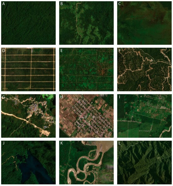
Figure 5. Examples of land cover classes for the GEOBIA classification. Each tile is extracted from the 2021 Q4 (September–December) Planet Visual Basemap. (A) Forest; (B) non-forest vegetation (light green); (C) wetland; (D,E) plantation; (F) exposed soil associated with roads and selective logging; (G) built-up areas with exposed soil, including new road construction; (H) mosaic of built-up areas and small-scale agriculture; (I) mosaic of built-up areas, agriculture, and remnant forest, with a river and a partially exposed riverbed visible; (J) deep water; (K) sediment-laden water; (L) forest in steep, high-relief terrain where extreme topography produces pronounced terrain-induced shadows.

2.4.2. Moderate-Spatial-Resolution Land Cover

To assess the impact of scale on the baseline land cover classification (Section 2.4.1), within the same 5 km buffers around the type localities for the year 2021, we developed a hierarchical classification workflow in GEE using a three-year (2019–2021) medoid composite derived from Landsat 8 Collection 2 surface reflectance data. Cloud cover was masked out by dilating the Landsat QA_pixel cloud and shadow bitmasks by 60 m (2 pixels). The final composite was generated using a medoid reducer to select the actual pixel observations closest to the multidimensional spectral median, ensuring spectral integrity.

Linear spectral mixture analysis was applied to the composite to derive fractional abundances for green vegetation (GV), non-photosynthetic vegetation (NPV), soil, and cloud endmembers. We also calculated a shade-normalized GV fraction (GV_S) [50] to help emphasize canopy structure and mitigate topographic effects (Equation (1)).

{G V}_{s} = \frac{G V}{(1 - s h a d e)}

(1)

Land cover was then assigned using a priority-based decision tree. First, any pixel with a cloud endmember fraction exceeding 0.4 was labeled as cloud, and water bodies were isolated by identifying pixels that simultaneously exhibited high shade abundance (shade ≥ 0.65) and low green vegetation abundance (GV ≤ 0.15), a combination characteristic of the low-reflectance properties of deep water. Next, following the ruleset defined by ref. [51], non-forest areas were identified where either the soil or NPV fractions represented the dominant spectral share (exceeding the GV fraction). Remaining pixels were classified as non-forest vegetation if they met the specific criteria defined in Equation (2) [51]:

0.56 < {G V}_{s} < 0.8 A N D

(2)

0.14 < N P V < 0.34 \land 0 < s o i l < 0.17 O R

{G V}_{s} < 0.8 a n d n o t p r e v i o u s l y i d e n t i f i e d a s N o n - f o r e s t

To ensure spatial cohesion, a post-classification majority filter was applied using a 3 × 3 pixel moving window, and the results were reprojected to the native 30 m Landsat pixel size. Final land cover areas were extracted for each 5 km buffer using the ee.Image.pixelArea() function.

2.4.3. Validation

We validated the high-resolution baseline classification through visual interpretation by expert remote sensing interpreters. A total of 747 thumbnails were extracted from the basemap, representing seven land cover classes: intact forest (n = 301), water (n = 88), soil (n = 76), plantation (n = 51), wetland (n = 87), non-forest vegetation (agriculture or natural) (n = 78), and built-up (n = 66), as seen in Figure 5. For each sample, a 30 m-diameter circle was drawn over the target land cover. Where the circle did not fully encompass the feature, a dot was placed within the circle to indicate the focal class. Following the approach of ref. [16], thumbnails were presented online using Survey Legend (Malmö, Sweden) across five separate surveys, each containing 51 questions. Before beginning, respondents reviewed instructions with example images for each land cover type. In each question, participants were shown a set of six thumbnails and asked to identify those corresponding to a specified land cover class (Figure 6). Each survey was independently completed by five expert interpreters. A sample was considered correctly classified if at least three of the five experts agreed with the GEOBIA classification label.

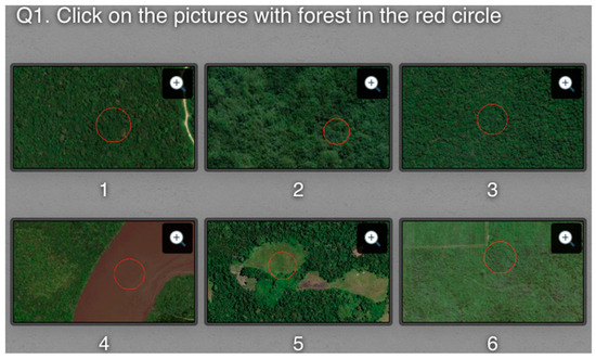
Figure 6. Example of one of the questions shown to the expert interpreters. The 30 m-diameter red circles represent the area to be examined.

2.4.4. Decadal Forest Change Analysis (1995–2025)

We used GEE to assess forest cover dynamics over a 30-year period within the same 5 km buffers around the type localities by implementing a multi-decadal change detection workflow using Landsat 4–9 Collection 2, Level 2 surface reflectance data. We defined four distinct epochs centered on 1995, 2005, 2015, and 2025, using a three-year temporal window for each to mitigate persistent cloud cover. Clouds and residual cloud edges were removed as described in Section 2.4.2. To synthesize representative cloud-free imagery while preserving the spectra, we generated composites using a medoid reducer, which selects the single actual pixel observation closest to the multidimensional median of all spectral bands.

Following the methodology described by ref. [50], linear spectral mixture analysis was performed on the epochal composites to decompose pixels into fractional abundances of GV, NPV, soil, and cloud endmembers. We then calculated the Normalized Difference Fraction Index (NDFI) (Equation (3)):

N D F I = \frac{{G V}_{s} - (N P V + s o i l)}{{G V}_{s} + N P V + s S o i l}

(3)

Forest change was quantified by computing the change in NDFI (

∆ N D F I)

between consecutive epochs (1995–2005, 2005–2015, and 2015–2025). Land cover change was categorized using a hierarchical classification logic. Transitions were classified as deforestation

(∆ N D F I \leq - 0.25)

, forest degradation/logging

(- 0.25 < ∆ N D F I \leq - 0.095)

, or vegetation regrowth

(∆ N D F I \geq 0.095)

. Pixels with an initial NDFI ≤ 0.3 were labeled as pre-existing non-forest to avoid false change detection in previously cleared areas. A stable forest was defined by a

∆ N D F I

between −0.095 and 0.095. To ensure spatial coherence, we applied a post-classification spatial majority filter using a 3 × 3 pixel window. Finally, class areas were calculated for each 5 km buffer using the ee.Image.pixelArea() function. To maintain the integrity of the decadal comparisons, a union masking strategy was employed for these classes. If a pixel was identified as cloud or water in either the starting or ending epoch of a specific transition period (e.g., 1995 or 2005), it was assigned to the respective “cloud” or “water” class in the final change map. This conservative approach ensured that remnant clouds or fluctuating water levels were not erroneously recorded as forest loss, degradation, or regrowth.

2.5. Time-Sequence Analysis of Disturbance

To determine disturbances in vegetation cover for species not associated with lakes or large rivers (Section 2.6), we used GEE to generate multi-decadal Normalized Difference Vegetation Index (NDVI) [52,53] time sequences within 300 m buffers of the type localities. The NDVI is a widely used spectral index derived from red and near-infrared reflectance that exploits the strong absorption of red light and high reflectance of near-infrared radiation by healthy vegetation, enabling the presence and density of vegetation to be mapped from remotely sensed imagery (Equation (4)):

N D V I = \frac{ρ N I R - ρ R e d}{ρ N I R + ρ R e d}

(4)

where

ρ N I R

is reflectance in the near-infrared band and

ρ R e d

is reflectance in the red band.

Landsat 4–9 Collection 2, Level 2 surface reflectance imagery (1984–2024) was retrieved and cloud-masked as described in Section 2.4.2. For each cloud-free acquisition, the mean and minimum NDVI were extracted within the 300 m buffer. The vectors representing the mean and minimum NDVI were analyzed in MATLAB v2025a (MathWorks, Natick, MA, USA). Missing values were first filled using a Modified Akima cubic Hermite interpolation based on ref. [54], which produces a smooth, shape-preserving curve while minimizing overshoot and oscillatory artifacts. Outliers were then detected using a 6-sample moving median window and replaced with interpolated values based on the same Modified Akima interpolation to maintain continuity in the series. The resulting time-sequences were smoothed using a third-degree Savitzky–Golay filter with a smoothing factor of 0.45–0.9 to reduce noise while preserving spectral shape. Divergence points were identified where the minimum NDVI exhibited a decreasing trend while the mean NDVI remained stable or increased, which we interpret as vegetation loss or disturbance in the vicinity of the type localities.

2.6. Surface Water Extent Classification

For species described from lakes (M. lacunosa, M. boesemani, M. kamaka, M. lakamora, M. parva, and M. sneideri) and large rivers (M. ericrobertsi and M. bowmani), surface water classifications were generated in GEE. The frequency of observation varied per species, based on image availability and cloud cover. For the smaller water bodies, a combination of RapidEye, PlanetScope Dove-R, and SuperDove imagery was used (Table 2). For the larger water bodies, the analyses were extended farther back in time with Landsat 5 and 7 Collection 2, Level 2 surface reflectance imagery (Table 2). As a visual comparison, for M. kamaka and M. lakamora, a satellite photograph with a nominal ground resolution of ~2.7–7.6 m from the declassified CORONA mission (KH-4A, panoramic J-1 camera) [55,56] taken on 29 June 1966 is included. Cloud cover precluded similar comparisons for other waterbodies.

Table 2. List of satellite imagery used for mapping the extent of surface water for the lake and large river species.

For the digital images listed in Table 2, surface water delineation was performed using an automated, multi-stage adaptive thresholding workflow implemented in GEE. The near-infrared (NIR) band was utilized as the primary spectral input due to the high absorptivity of water in this wavelength range and to ensure band consistency across all satellite sensors. A preliminary manual threshold (7.75%) was applied to isolate candidate water-pixels. From this constrained distribution, a global Otsu threshold was calculated to segment the image into an initial binary water mask [57]. To improve the precision of the water–land interface, an adaptive refinement strategy was employed. First, canny edge detection was applied to the global mask, and the resulting edges were buffered to sample the localized spectral transition between land and water. A secondary, adaptive Otsu threshold was then recalculated specifically for these buffered edge zones to resolve boundary ambiguities [57]. Given that Otsu thresholding relies on histogram separability [58], this single-band approach supports stable cross-sensor application, whereas index-based methods often require additional scene-dependent logic to achieve robustness across space and time [59]. The resulting raster masks were smoothed using a spatial mode filter with a 3, 5, or 30 m radius kernel (depending on the sensor). Finally, the processed masks were converted into vector polygons, and an area-based filter (minimum threshold of 8100 m²) was applied to retain contiguous water bodies.

3. Results

3.1. Cloud Cover

Cloud-free Landsat data availability exhibited pronounced spatial heterogeneity across the study area (Figure 7). In individual years (Figure 7B,C), large portions of the region were characterized by relatively few cloud-free acquisitions, with extensive areas receiving fewer than ~10–20 usable observations, particularly in persistently cloudy interior zones such as the Arfak Mountain Range and the Lengguru Foldbelt. The linear features visible in the acquisition-density maps correspond to overlaps between adjacent Landsat paths and rows, where increased revisit frequency results in locally elevated observation counts. These overlaps were particularly fortuitous for a few of the small island species M. catherinae, M. batanta, and M. salawati (Figure 1, map # 1, 3, and 4), as well as M. ericrobertsi and M. manibuii (Figure 1, map # 8 and 21) from the Bird’s Head region. Data availability was broadly similar between individual years (e.g., 2014 versus 2021), with substantial areas of the landscape remaining sparsely observed at annual timescales (maximum values < 50). These results are similar to those found by ref. [60] with a range of yearly valid cloud-free optical satellite images (combining both the Landsat and Sentinel-2 archives) from the type locality of M. sneideri, ranging from 0 to 7 (2017–2021), increasing to 17–41 valid observations for M. catherinae over the same period.

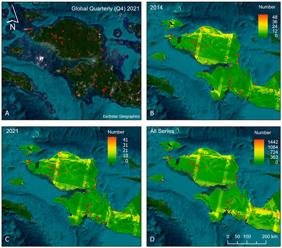
Figure 7. (A) Planet Labs visual basemap mosaic for the fourth quarter (October–December) of 2021 (global_quarterly_2021q4_mosaic). (B) Total number of cloud-free Landsat observations in 2014 derived from Landsat 7–9 Level 2, Collection 2 data. (C) Total number of cloud-free Landsat observations in 2021 derived from Landsat 7–9 Level 2, Collection 2 data. (D) Total number of cloud-free Landsat observations accumulated from 1984 to 2024 across Landsat 4–9 Level 2, Collection 2 data. Red points indicate the locations of the type localities.

When aggregated across the full Landsat archive (1984–2024) (Figure 7D), the number of cloud-free observations exceeded 1000 acquisitions in a few localized path/row overlap areas; however, most of the landmass accumulated fewer than 300 cloud-free observations over the full period (average of 7.5/year), which is just over the minimum of 7 recommended by ref. [61] for time-series analysis. These patterns demonstrate that long-term compositing is essential to mitigate chronic cloud contamination and to ensure robust detection of land cover change in this region.

Even the cloud-minimized Planet quarterly basemap mosaic (Figure 7A) used to generate the high-resolution baseline classification contained residual cloud and haze artifacts in some areas, such as the Pegunungan Kumawa Nature Reserve, where M. sneideri is found, and at a high elevation in the Lengguru Foldbelt, reflecting the persistent atmospheric limitations of optical remote sensing in this region. This residual contamination limited the availability of truly “wall-to-wall” cloud-free observations at fine spatial scales and highlights the importance of multi-temporal compositing, classification, and change-detection methods that minimize sensitivity to residual cloud and haze.

3.2. Land Cover Change

3.2.1. Baseline Land Cover

The accuracy assessment results (Table 3) indicate a high overall classification performance for the GEOBIA approach with the Planet visual basemap, with class labels showing strong agreement with interpretations by expert remote sensing analysts. The highest accuracies were obtained for the built-up and plantation classes, which exhibited no commission or omission errors, and for water, which showed only a small commission error (3.4%). These classes are readily distinguishable based on color and texture and are also easily recognized by human interpreters. Forest cover was likewise mapped reliably, with both commission and omission errors of only 1.7%.

Table 3. Accuracy assessment results from the expert visual interpreter surveys of the baseline classification generated from the 2021 global quarterly cloud-minimized basemap from PlanetLabs.

Soil, wetland, and non-forest vegetation exhibited comparatively lower accuracies; however, all retained overall accuracies from 85.9% to 89.7%. Confusion was most frequent between wetland and non-forest vegetation classes, reflecting the inherently fuzzy ecological boundary between these cover types, where shrubs and grasses commonly occur in both.

Class composition within the 5 km type locality buffers was broadly consistent between the Landsat 8 OLI and PlanetLabs visual basemap classifications (Figure 8) for the year 2021, with forest comprising the dominant land cover class for all species. Across species, total forest area estimates derived from the two classifications were similar, with the Landsat-based classification overestimating forest extent by approximately 14,254 ha (308,785 ha versus 294,531 ha). The most prominent differences between the two were concentrated in the non-forest subclasses (non-forest vegetation, non-forest, water, and wetland), which together represented a small proportion of total area but exhibited greater inter-sensor variability (Figure 8 and Figure 9). Within the 5 km buffers, the GEOBIA classification of the visual basemap identified 2938.9 ha of cleared land (non-forest), whereas the Landsat classification accounted for only 31.0 ha, indicating that 99% of fine-scale clearing detected at high-spatial resolution is not resolved as a distinct class in the 30 m pixel Landsat-based classification. Additionally, the visual basemap classification identified 1120.5 ha of wetland, whereas no wetland area was mapped in the Landsat-based classification. This result is not surprising, as the spectral mixture analysis applied to the Landsat imagery incorporates wetlands into the class with high proportions of green vegetation (GV), which in this study is interpreted as forest.

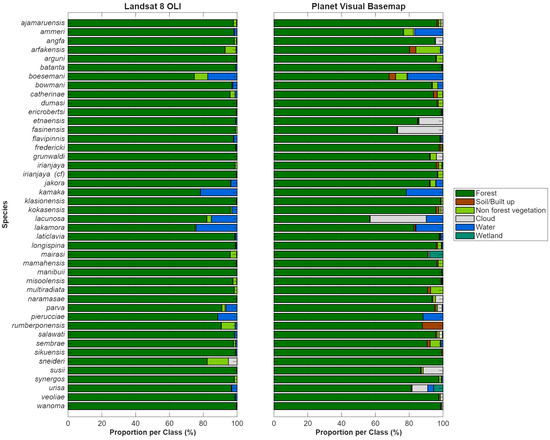
Figure 8. Comparison of land cover class composition within 5 km buffers surrounding type localities derived from Landsat 8 OLI and Planet visual basemap classifications.

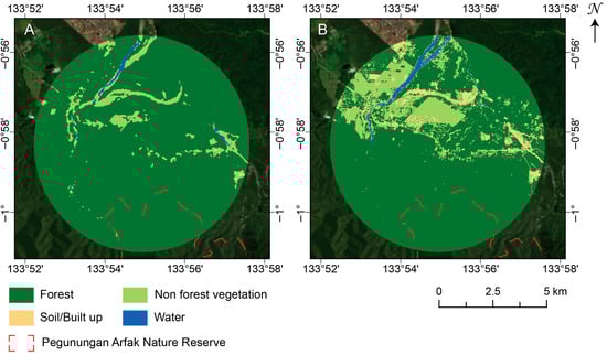
Figure 9. Example land-cover classifications within the 5 km buffer surrounding the type locality of M. arfakensis for 2021, derived from (A) Landsat 8 OLI composite processed in GEE using spectral mixture analysis, and (B) GEOBIA classification of the Planet Visual Basemap (Q4, September–December 2021). The background image is the 2021 Q4 Planet Visual Basemap.

On a species level, the largest discrepancies were observed for those whose habitats have larger proportions of cleared land, either as soil from clearing, roads, or settlements: M. arfakensis (Figure 9), M. boesemani, M. catherinae, M. dumasi, M. fredericki, M. kokasensis, M. misoolensis, and M. sembrae, resulting in an underestimation of landscape heterogeneity and non-forest cover. The comparison between classifications for M. arfakensis (Figure 9) clearly demonstrates that only the largest patches of non-forest vegetation are detected in the Landsat classification. Areas of cultivated fields with high biomass are frequently misclassified as forest in the Landsat results due to a strong green-vegetation (GV) component. Figure 9B (Planet basemap) also reveals substantially greater spatial fragmentation of non-forest vegetation and soil/built-up areas, particularly along field margins, roads, and settlement edges. In contrast, Figure 9A (Landsat) generalizes these features into larger, more homogeneous forest patches. This highlights the loss of fine-scale edge and patch structure at moderate-spatial resolution. Linear features (e.g., roads and narrow clearings) are clearly resolved in the Planet basemap classification but are largely absent or discontinuous in the Landsat result, with implications for detecting early-stage disturbance and infrastructure expansion with a higher likelihood of underestimation from moderate-resolution imagery. The river is consistently detected in both classifications, but the Planet basemaps provide clearer delineation of adjacent land cover context (e.g., exposed banks). Importantly, the Landsat classification may overestimate forest connectivity and underrepresent anthropogenic disturbance. An example of differences due to natural origins is for M. rumberponensis. The summit of Rumberpon Island, which has grassland surrounding exposed soil/rocks, was classified as non-forest vegetation from the Landsat composite (due to the presence of the grassland) but was classified as non-forest due to the exposed soil/rocks from the Planet basemap. Overall, these differences indicate that moderate-resolution Landsat classifications capture broad land cover patterns but underestimate fine-scale disturbance, landscape fragmentation, and edge complexity relative to high-resolution Planet basemaps.

The complicating influence of cloud cover is clear in the Landsat results for M. sneideri. Although the area surrounding the spring is entirely forested, approximately 5% of the Landsat composite is obscured by clouds, and cloud edges further confounded the spectral mixture analysis, leading to ~13% of the area being classified as non-forest vegetation. Cloud contamination also affected the high-resolution Planet visual basemap classifications, most notably for M. lacunosa, where 33% of the analysis area was obscured. Similarly, cloud cover masked 26.8% and 14.1% of the area for M. fasinensis and M. etnaensis, respectively. In total, 15 type localities exhibited residual cloud cover within the high-resolution classification areas.

Figure 10 illustrates examples of small-scale land cover disturbances as observed on the ground. The most common include road construction (Figure 10A), land clearing (Figure 10B), and timber harvesting (Figure 10F). Urban development (Figure 10D) is most prominent near the type localities of M. arfakensis, M. boesemani, M. multiradiata, M. cf. irianjaya, and M. sembrae. Oil palm plantations (Figure 10E) are encroaching on the habitat of M. longispina and are also present near the 5 km buffer surrounding the type locality of M. arfakensis. An important aspect of habitat alteration not captured by any remote sensing product is illustrated in Figure 10E. Local villagers are culturing tilapia cichlids (Oreochromis niloticus) in cages within Wensi Creek, near the type locality of M. ajamaruensis. Escaped individuals disperse throughout the river system, representing a source of biological disturbance that cannot be detected using remotely sensed observations.

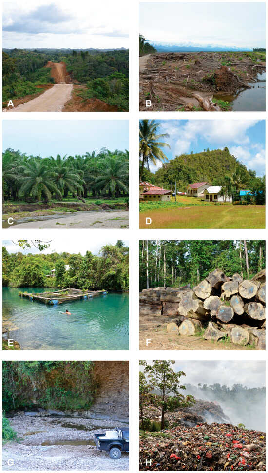
Figure 10. Examples of the land cover changes found throughout Western New Guinea: (A) road construction from Teminabuan to Ayamaru village in 2013; (B) deforestation in the Arfak region; (C) palm oil plantation near Manokwari. (D) Sasnik village on the Central Ayamaru Plateau. (E) The Wensi Creek (Kali Wensi) and its smaller affluents are the type locality of Melanotaenia ajamaruensis. The villagers are culturing Tilapia cichlids, Oreochromis niloticus, in cages in this river, from which the cichlids easily escape and spread throughout the whole river system. (F) Pile of illegally cut timber logs in the north of Bird’s Head Peninsula, officially a protected area (Tamrau Utara Nature Reserve). (G) Water abstraction at the type locality of M. klasioensis from a concrete factory located upstream. (H) Landfill near the city of Sorong.

3.2.2. Decadal Forest Change Analysis (1995–2025)

Results from the decadal forest-change analysis indicate that the 1995–2005 period experienced the highest levels of deforestation and disturbance within the 5 km buffers surrounding the type localities of most species, relative to the 2005–2015 and 2015–2025 epochs (Figure 11). An exception is M. catherinae, for which deforestation and disturbance coincide with the construction and subsequent expansion of Marinda Airport (RJM) between 2007 and 2014 [62]. For M. grunwaldi and M. cf. irianjaya, the 2005–2015 period also exhibited elevated levels of disturbance and forest loss. The type locality of M. grunwaldi lies between the city of Nabire and the town of Topo, where extensive small-scale clearing and regrowth are evident along a secondary road extending northwest from Topo toward Nabire, as well as along the Topo River, a tributary of the larger Wami River system. The Wami River and its major tributaries are highly turbid due to artisanal and small-scale gold mining (ASGM) along their banks. These ASGM activities are widespread south of Nabire, where small, informal mining operations are concentrated along river systems and are associated with localized deforestation, sediment disturbance, and often mercury use [63,64].

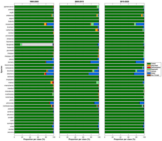
Figure 11. Multi-decadal forest change detection derived from the Landsat 4–9 Collection 2, Level 2 surface reflectance archive. Forest loss, disturbance, and regrowth were quantified across three epochs (1995–2005, 2005–2015, and 2015–2025) using a spectral mixture analysis change detection framework.

The 5 km buffer surrounding the type locality of M. cf. irianjaya lies south of, but partially overlaps with, the village of Hasik Jaya (SP II). The designation “SP” refers to Satuan Permukiman, a transmigration settlement unit, and “II” denotes the phase of development; thus, SP II represents the second planned transmigration settlement established in the Hasik Jaya area. For M. arfakensis, for which degradation and deforestation are seen across all three periods, the 5 km buffer intersects one of the rice production units (SP I) near Prafi Mulia village in Prafi District [65]. The buffer is also proximal to the city of Manokwari, the provincial capital of West Papua. The Prafi–Warmare–Maruni road dissects the buffer, linking the rice production area to the coast, and is associated with linear infrastructure development and agricultural activity along its corridor. This road is clearly seen in Figure 9B but is only discontinuously captured at the moderate resolution in Figure 9A.

3.3. Fine-Scale Forest Loss

Small-scale deforestation events were detected within 300 m buffers surrounding the type localities of multiple species (Figure 12). These events were expressed as divergence points in the NDVI time-sequence, characterized by decreases in minimum NDVI, while mean NDVI remained stable or increased, indicating localized clearing/vegetation loss (Figure 13, Figure 14 and Figure 15). The timing and frequency of these events varied among type localities, with some exhibiting multiple disturbance events over the Landsat record, while others showed none that could be reliably identified. No NDVI divergence points were identified for M. dumasi, M. manibuii, M. misoolensis, M. sikuensis, M. synergos, and M. urisa, and these were therefore omitted from Figure 12. Apparent temporal trends in disturbance frequency should be interpreted cautiously because the cloud-masked Landsat time-sequence is uneven through time, with lower observation density in earlier decades potentially reducing the detectability of short-duration events. For M. arfakensis, M. mamahensis, and M. cf. irianjaya, disturbance events corresponded to visually identifiable land cover changes in available cloud-free RapidEye and PlanetScope imagery (Figure 13, Figure 14 and Figure 15), providing qualitative corroboration of the time-sequence signals.

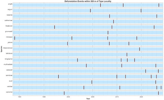
Figure 12. Small-scale deforestation events were detected within 300 m buffers surrounding the type localities of species not described from large lakes or rivers. Vertical bars indicate deforestation events in which the minimum NDVI time-sequence decreased while the mean NDVI remained stable or increased. Three species (M. arfakensis, M. mamahensis, and M. cf. irianjaya), for which cloud-free RapidEye and/or PlanetScope imagery was available to visually corroborate these events, are illustrated separately in Figure 13, Figure 14 and Figure 15.

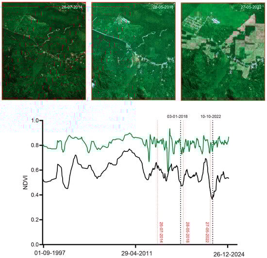
Figure 13. Time-sequence of mean NDVI (green) and minimum NDVI (black) within a 300 m radius of the type locality of M. arfakensis. Black dotted lines indicate the dates (DD-MM-YYYY) corresponding to the peaks of the identified disturbance events (3 January 2018 and 10 October 2022). Red dotted lines mark the acquisition dates of high-resolution satellite imagery available prior to and near these events, including RapidEye (26 July 2014) and PlanetScope imagery (Dove-R on 28 May 2018 and SuperDove on 27 May 2022).

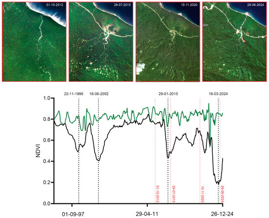
Figure 14. Time-sequence of mean NDVI (green) and minimum NDVI (black) within a 300 m radius of the type locality of M. mamahensis. Black dotted lines indicate the dates (DD-MM-YYYY) corresponding to the peaks of the identified main disturbance events (22 November 1998, 18 June 2002, 29 January 2015, and 18 March 2024). Red dotted lines mark the acquisition dates of high-resolution satellite imagery available prior to and near these events, including RapidEye (1 October 2012, 29 July 2015) and PlanetScope imagery (Dove-R on 10 November 2020 and SuperDove on 29 June 2024).

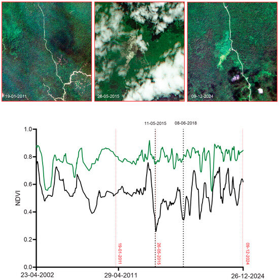
Figure 15. Time sequence of mean NDVI (green) and minimum NDVI (black) within a 300 m radius of the type locality of M. cf. irianjaya. Black dotted lines indicate the dates (DD-MM-YYYY) corresponding to the peaks of the identified main disturbance events (11 May 2015 and 8 June 2018). Red dotted lines mark the acquisition dates of high-resolution satellite imagery available prior to and near these events, including RapidEye (19 January 2011 and 26 May 2015) and PlanetScope imagery (SuperDove on 9 December 2024).

For M. arfakensis (Figure 13), the 300 m buffer lies outside the rice production units near Prafi Mulia village but nonetheless exhibits evidence of localized clearing. In 2018, small field-scale clearings are visible relative to the 2014 baseline, while by 2022 one side of the stream north of the Prafi–Warmare–Maruni road is entirely cleared. For M. mamahensis (Figure 14), timber extraction roads are visible by 2015, compared to 2012, when the forest surrounding the creek appeared undisturbed. Clearing and construction activity are also evident near the bridge crossing the creek in 2015. By 2020, portions of the timber extraction road network show signs of regeneration, and a new bridge is visible immediately south of the original crossing. In 2024, renewed construction activity and recent forest clearing are evident in the vicinity of the bridge. For M. cf. irianjaya, small-scale timber extraction is visible in the 2011 RapidEye imagery, while the forest surrounding the stream otherwise remains largely intact (Figure 15). By 2015, a large clearing is evident through a break in cloud cover, extending across both sides of the stream, where the streambed becomes clearly visible. By 2024, the cleared area appears to have been abandoned, with forest regeneration underway and timber extraction roads largely no longer discernible.

3.4. Surface Water

Figure 16, Figure 17, Figure 18 and Figure 19 illustrate surface water extent extracted for lakes and rivers (Table 2). For the M. boesemani type locality, surface water area varies substantially, ranging from 2.5 km² on 26 April 2017 to 37.9 km² on 23 December 2024. Although part of this variability likely reflects seasonal fluctuations, imagery from 12 April 2024 indicates a surface water extent of 15.6 km² for Lake Ayamaru, suggesting that interannual variability is also present. Because surface water mapping relied on optical satellite imagery, total water extent may be underestimated where aquatic vegetation obscures open water [66]. Photographs in ref. [67] document pronounced seasonal changes in water level, as well as extensive floating aquatic vegetation and large beds of submerged macrophytes (Potamogeton sp. and Vallisneria sp.). Even prior to large-scale land cover change around the series of lakes, seasonal water-level variation of approximately 0.5 m was reported, with high water clarity supporting extensive submerged vegetation and seasonal transitions of lake margins to marsh grasslands [68]. Several freshwater springs along the lake margins contribute to the lake system; however, some have become algae-laden and exhibit degraded water quality in recent years [67]. Recent local assessments further report that substantial portions of Lake Ayamaru have experienced drying and contraction, attributed to sedimentation and erosion processes, hydrological modification, and land use pressures in the surrounding catchment [67,69].

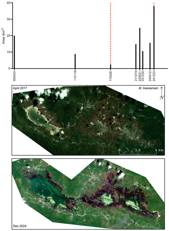
Figure 16. Surface water extent at the type locality of M. boesemani as mapped from optical satellite imagery (Landsat 7 ETM+, RapidEye, and PlanetScope Dove-R and SuperDove). Black bars indicate the total mapped surface water area (km²) for each observation date (YYMMDD). Dashed red lines denote dates for which corresponding satellite imagery is shown. The low water level observed in the April 2017 RapidEye image is characterized by bright, exposed shoreline sediments, whereas the high water level in the December 2024 PlanetScope SuperDove image shows a greater extent of surface water, as well as extensive exposed aquatic vegetation beds (light green).

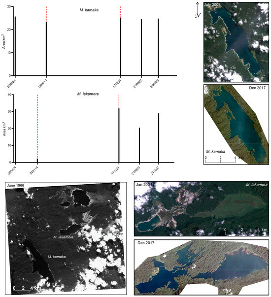
Figure 17. Surface water extent of Lake Kamakawaiar, the type locality of M. kamaka, and Lake Lakamora, the type locality of M. lakamora, as mapped from optical satellite imagery (Landsat 5 TM and PlanetScope Dove-R and SuperDove). Black bars indicate the total mapped surface water area (km²) for each observation date (YYMMDD). Dashed red lines denote dates for which corresponding satellite imagery is shown. A historical satellite photograph (June 1966) from the CORONA KH-4A mission is included for visual comparison prior to the availability of modern digital satellite imagery.

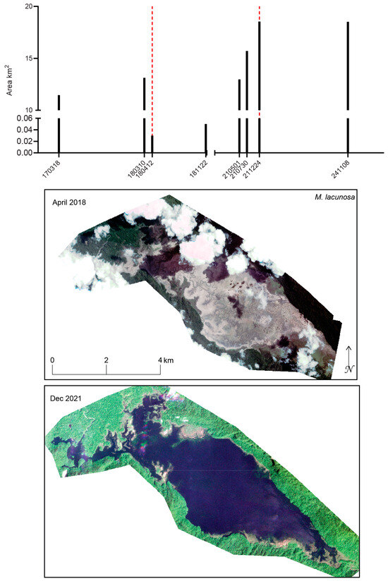
Figure 18. Surface water extent of the Mbuta Basin, into which the streams draining the type locality of M. lacunosa flow, as mapped from PlanetScope Dove-R and SuperDove imagery. Black bars indicate the total mapped surface water area (km²) for each observation date (YYMMDD). Dashed red lines denote dates for which corresponding satellite imagery is shown.

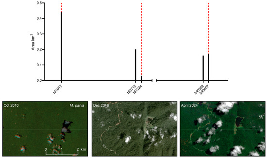
Figure 19. Surface water extent of Lake Kurumoi, the type locality of M. parva, as mapped from optical satellite imagery, including RapidEye, PlanetScope Dove-R, and SuperDove imagery. Black bars indicate the total mapped surface water area (km²) for each observation date (YYMMDD). Dashed red lines denote dates for which corresponding satellite imagery is shown.

Water levels in Lake Kamakawaiar, the type locality for M. kamaka, appear to have remained relatively stable across seasons and years, with mapped surface water extent ranging from 23.3 km² on 11 July 2005 to 25.7 km² on 24 April 2000 (Figure 17). Only a narrow ring of exposed rock [70] is visible in the low-water image from July 2005. The historical satellite photograph from 1966 shows a water level comparable to modern observations, potentially reflecting the lake’s depth, estimated at approximately 50 m [71]. In contrast to many other Indonesian lakes, the Triton Lakes system, of which Lake Kamakawaiar is a part, remains comparatively poorly studied [71]. Also part of the Triton Lakes system is Lake Lakamora (Figure 17), the type locality for M. lakamora. In contrast to Lake Kamakawaiar, surface water extent at Lake Lakamora varies substantially, ranging from a minimum of 2.3 km² on 14 January 2004, when water is present primarily in likely the deepest portion of the basin, to a maximum of 31.9 km² on 24 December 2017. The historical satellite photograph from 1966 (Figure 17) corroborates that this large variability in water level is a natural process, with surface water at that time limited largely to the western and central portions of the lake.

Of all the water bodies examined in this study, the Mbuta Basin, into which the streams draining the type locality of M. lacunosa flow, exhibits the most extreme variation in surface water extent (Figure 18). We focus on basin-scale water levels because the holotype and most paratypes were collected there [33]. This area was extremely remote and was accessible only by helicopter under favorable weather conditions until the coastal village of Kaimera and a road linking it to the basin were constructed beginning in 1992. The minimum surface water extent recorded was 0.03 km² on 12 April 2018 and 0.05 km² on 22 November 2018, whereas maximum extents of 18.54 km² and 18.52 km² were observed on 24 December 2021 and 8 November 2024, respectively. Because both minimum and maximum extents occurred during similar times of year, seasonality alone is unlikely to explain the magnitude of these changes. During low-water periods, the outlines of stream beds are visible within the basin, suggesting that shallow water may persist outside of the larger ponds. A photograph taken in April 1997 shows the basin surface as a marsh with small ponds and grasses described as 3–4 m tall, with type specimens collected from a creek up to 2 m deep [33]. In contrast, conditions in December 2013 were described as markedly different, with the basin resembling a continuous lake [33]. Located within the Lengguru Foldbelt, the region’s karst geology strongly suggests that the Mbuta Basin drains primarily through underground systems. Carbonate anticlines are separated by deep valleys that are locally closed and rifted, resulting in basins without surface outflow (i.e., endorheic systems), a defining characteristic of the Lengguru karst [26]. The Lengguru expeditions documented limestone karsts extending into the Ceram Sea to depths of ~120 m [29,72], suggesting that underground drainage from inland basins may re-emerge as submarine springs near Etna Bay. However, the subsurface drainage pathway from the Mbuta Basin has not yet been traced.

The surface water extent of Lake Kurumoi (Figure 19), the type locality of M. parva, also exhibits variability, ranging from a minimum of 0.03 km² on 24 December 2016 to a maximum of 0.44 km² on 12 October 2010. However, as with the surface water extent results for the Ayamaru Lakes (Figure 16), aquatic vegetation may obscure the true extent of open water in optical satellite imagery. The original species description reports dense stands of Ceratophyllum demersum in parts of the lake [34].

Similarly to Lake Kurumoi (Figure 20), the full surface-water extent of the high-altitude (∼1050 m) spring in the Kumawa Mountains that constitutes the type locality of M. sneideri may be substantially obscured by aquatic vegetation in optical satellite imagery (Figure 20). The species description notes that during the dry season, surface water is confined to a small spring emerging from limestone bedrock (approximately 1–2 m wide and 10–20 cm deep), which flows for ~600 m across the basin before draining back underground [73]. During periods of heavy rainfall, surface water expands and a small lake forms within the basin.

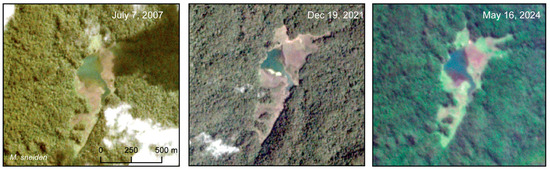
Figure 20. PlanetScope Dove-R and SuperDove imagery of the basin forming the type locality of M. sneideri. A small creek emerges from limestone bedrock and drains across the basin to form a small lake.

The two species described from large river systems (Figure 21), M. bowmani from the Siriwo River and M. ericrobertsi from the Kladuk River system, exhibit contrasting patterns in surface water extent. The Siriwo River shows pronounced seasonality, with the mapped surface-water area along the 5 km reach ranging from 1.33 km² on 6 December 2017 to 2.01 km² on 9 August 2021, along with differences in water clarity. In contrast, the surface water area mapped for the 5 km reach of the Kladuk River varies only slightly, from 0.38 km² on 23 December 2014 to 0.41 km² on 16 November 2024.

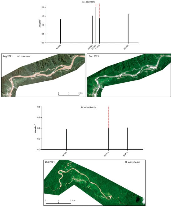
Figure 21. Surface extent of 5 km reach of the Siriwo River, the type locality of M. bowmani, and of the Kladuk River, the type locality of M. ericrobertsi, as mapped from optical satellite imagery (PlanetScope Dove-R and SuperDove). Black bars indicate the total mapped surface water area (km²) for each observation date (YYMMDD). Dashed red lines denote dates for which corresponding satellite imagery is shown.

4. Discussion

We show that land cover change around rainbowfish type localities is highly dynamic, spatially localized, and frequently undetected by moderate-resolution imagery, despite its ecological relevance for narrowly distributed freshwater species. Remote sensing provides a powerful means of assessing land cover change and potential threats to freshwater fish habitats across broad geographic areas; however, applications for restricted-range species impose particularly stringent requirements on spatial and temporal resolutions [74].

As described by ref. [22], Western New Guinea is among the most persistently cloudy regions on Earth, where cloud cover is a primary factor limiting the availability and quality of optical remotely sensed data. Persistent cloud cover (Figure 7; see examples in Figure 15, Figure 17 and Figure 18) thus emerges as a dual constraint, both reducing the number of usable optical observations and actively confounding land cover classification through cloud edges and haze. For the type localities of some species, such as M. sneideri, certain years contain no usable cloud-free observations from moderate-resolution EO systems [60]. The impact of this limitation is illustrated in Figure 8, where forest cover was erroneously classified as non-forest vegetation due to residual cloud and cirrus contamination in the Landsat imagery. The high temporal revisit frequency (near-daily) of satellite constellations such as PlanetScope can partially mitigate these challenges; however, as shown in Figure 1, even the least cloudy quarterly basemap mosaics still contain residual cloud cover. For some type localities, including M. lacunosa, M. fasinensis, and M. etnaensis, clouds obscured up to 33% of the 5 km buffers. One potential mitigation strategy would be to extend the compositing window from quarterly to annual periods by selecting the clearest pixels from monthly mosaics or daily imagery for these areas.

Our results also clearly demonstrate that spatial resolution fundamentally shapes interpretations of land cover change around rainbowfish type localities. Moderate-resolution Landsat classifications (30 m pixel size) capture general forest cover patterns but systematically fail to resolve fine-scale disturbances, including small agricultural clearings, narrow roads, settlement edges, and localized soil exposure (Figure 8 and Figure 9). These features are detected in the high-resolution visual basemap GEOBIA classification, indicating that disturbance relevant to small freshwater habitats can be effectively invisible at Landsat scales. For narrowly distributed species, the minimum mapping unit of Landsat and similar moderate-resolution systems often exceeds the spatial footprint of ecologically meaningful change. This effect has also been demonstrated elsewhere, where landscape features that cannot be resolved in moderate-resolution imagery become detectable with increased spatial detail [75].

An important consideration is that pixel size does not correspond directly to the area on the ground contributing energy to a given pixel. For all optical EO sensors, the effective ground area influencing each pixel is substantially larger than the nominal pixel dimensions. This area is described by the point spread function (PSF), a two-dimensional function describing the spatial response of the imaging system in both the along-track and across-track directions, and effectively introduces spatial blurring [76]. The PSF integrates the combined effects of sensor optics, detector characteristics, platform motion, and onboard electronics [76]. Atmospheric conditions at the time of image acquisition, including turbulence and aerosol loading, further influence the effective spatial response [77]. In practical terms, each 30 m Landsat pixel represents a weighted integration of reflected energy originating from an area larger than 30 m × 30 m. The same principle applies to higher-resolution systems, although the specific PSF characteristics vary among sensors. For satellite constellations such as PlanetScope and RapidEye, these characteristics also vary slightly between individual spacecraft. Consequently, fine-scale or spatially localized land-cover changes may be poorly resolved or entirely obscured in moderate-resolution imagery, particularly when disturbance features approach or fall below the effective spatial resolution of the sensor.

Overall, our results show that the moderate resolution Landsat classification tends to generalize heterogeneous landscapes around type localities with clear anthropogenic influence into large, contiguous forest patches, leading to an overestimation of forest connectivity and an underrepresentation of fragmentation, particularly within mosaics of agriculture, settlement, and remnant forest. This effect is clearly illustrated at the type locality of M. arfakensis (Figure 9), where the Planet visual basemap resolves fragmented land use that is interpreted as continuous forest in the Landsat classification. These findings underscore the importance of high-spatial-resolution imagery for capturing small-scale and temporally transient land cover change events in Western New Guinea. Previous studies (e.g., refs. [78,79]) have demonstrated the value of monthly PlanetScope mosaics made available through Norway’s International Climate and Forest Initiative (NICFI). Although the NICFI program was not renewed in 2025, Planet Labs subsequently launched the Tropical Forestry Observatory, which continues to provide monthly PlanetScope mosaics over tropical forests for non-commercial use [80].

Analysis of decadal land cover change (Figure 11) and NDVI-based time sequences (Figure 12, Figure 13, Figure 14 and Figure 15) show that land cover change around rainbowfish type localities neither follows a simple trajectory of progressive deforestation, nor conforms to the temporal signatures typically exploited by time-series deforestation algorithms such as Continuous Change Detection and Classification (CCDC) [81]. Instead, disturbance is episodic, characterized by localized pulses during specific years associated with infrastructure development, settlement expansion, or extractive activities, and in some cases followed by partial or apparent regrowth. However, it is important to consider that a loss in greenness (as indicated by the minimum NDVI) may also reflect non-anthropogenic processes, including canopy gap dynamics following tree mortality or windthrow events [82,83]. This pattern contrasts with more uniform frontier-expansion narratives reported for countries such as Brazil [84] and Madagascar [85], underscoring the importance of temporal context when interpreting long-term change.

Across type localities (Figure 11, Figure 12, Figure 13, Figure 14 and Figure 15), land cover change is driven by multiple spatially distinct processes, including road construction, built-up area expansion, smallholder agriculture, logging, and alluvial mining that operate at different spatial scales and affect aquatic habitats through mechanisms such as increased sediment loading, hydrologic alteration, riparian disturbance, and changes in water quality [86,87,88,89]. Although species-specific ecological studies remain limited for many rainbowfishes, refs. [90,91] highlight the importance of riparian habitat for maintaining M. arfakensis populations in the Nimbai River. They report that canopy cover moderates stream temperatures and contributes leaf litter that supports the riverine food web. Riparian vegetation also supports reproduction by providing substrates for egg attachment and by creating sheltered nursery habitats for larvae. While this current study evaluated the presence of land cover change with the buffers, future studies should expand the spatial analysis and quantify where within a given buffer the change has occurred (e.g., within a riparian zone vs. upland). Loss of forest cover closer to streams could indicate a greater impact on water temperature and sediment input.

Exploration and discovery of Melanotaenia species in Western New Guinea have historically been tightly coupled to physical access. Field surveys have largely followed access corridors created by logging, agriculture, and mining activities, which open roads into otherwise remote forest regions, or have relied on helicopter-supported expeditions (e.g., refs. [73,92]). Even large-scale terrestrial biodiversity assessments indicate that extensive areas of Western New Guinea remain biologically unexplored (e.g., ref. [23]), highlighting a strong accessibility-driven sampling bias. Most ichthyological exploration in the region has occurred since the 1980s, with many Melanotaenia species described only within the last 15 years (Figure 3). The number of undescribed and likely new species is already estimated to exceed the number of currently described taxa (Figure 1), and additional species descriptions within Melanotaenia are expected in the coming years. More than half of the Melanotaenia species collected by the Lengguru expedition in 2014 are likely new species [29]. Exploration by local aquarium exporters and enthusiasts, facilitated by improved access and amplified through social media, is likely to further accelerate species discovery. While overcollection for the ornamental trade has posed documented risks for some species (e.g., M. boesemani) [93], for many narrowly distributed taxa the dominant threats arise instead from habitat loss and degradation associated with mining, logging, agricultural expansion, and introduction of non-native species (discussed below) [67,94,95]. Importantly, most Melanotaenia currently traded in the aquarium industry are captive-bred either by commercial farms or hobbyists due to the logistical challenges of wild collection and the ease of captive reproduction [93]. This suggests that habitat degradation, rather than harvest pressure, represents the primary long-term risk for many species.

The coupling between access, discovery, and disturbance is further reinforced by Indonesia’s Transmigrasi program, which relocated populations from densely populated islands such as Java and Sulawesi to frontier regions of Western New Guinea [68,96]. Planned transmigration settlements (SP I, SP II, etc.) were typically established in sparsely populated areas and are strongly associated with localized land cover change, including forest clearing for housing, roads, and agriculture, the largest economic sector in the region. Although centrally funded transmigration expanded most rapidly during the late New Order period and declined following the mid-1980s oil-price collapse, settlement footprints and associated land use dynamics persisted [97]. In the 2010s–2020s, transmigration was increasingly embedded within broader frontier development strategies, such as the Merauke Integrated Food and Energy Estate (MIFEE), which led to the allocation of large agribusiness concessions and spatially heterogeneous land cover change, even though the program did not achieve its original mega-estate vision at scale [98].

Over the past three decades, the Bird’s Head region, and particularly the Central Ayamaru Plateau, has experienced substantial human pressure with pronounced impacts on native flora and fauna. Areas surrounding the Ayamaru lakes, the city of Teminabuan, and adjacent parts of the plateau have attracted increasing numbers of settlers from other Indonesian islands, often accompanied by the introduction of non-native plants and animals. Several introduced fish species, including Trichopodus trichopterus, Aplocheilus panchax (via eggs adhering to rice plants), and widely distributed aquaculture species such as Cyprinus carpio, Oreochromis niloticus, and the predatory snakehead Channa striata, now compete directly with native fish communities. For example, C. striata is abundant in tributaries of the Ayamaru Lakes, where it preys on M. boesemani and other native species [67]. Lake Ayamaru faces further interacting pressures such as hydrological modification associated with recent dam construction, water-level variability, and shoreline disturbance from road and settlement expansion [67].

The Kaliwensi River, the only known habitat of M. ajamaruensis, is threatened by tilapia (Oreochromis niloticus) escaped from aquaculture cages. Although tilapia is not predatory, they can outcompete native species for resources, introduce pathogens, and alter water quality and substrate conditions. As of April 2024, Lake Kurumoi, the only known habitat of M. parva, remains isolated, with no direct road access to its shoreline. When type specimens were collected in 1989, the African cichlid Oreochromis mossambicus was already present. Although its introduction pathway remains unclear, it may date to colonial-era fisheries introductions, similar to those documented in the Ayamaru Lakes during the late 1930s and 1950s [34,68]. The Mbuta Basin, home to several endemic Mogurnda species as well as Pelangia mbutensis and M. lacunosa, is likewise threatened by the introduction of tilapia and other non-native fish species. Remote sensing is unable to capture the introduction of alien species and pathogens, but the emergence of smallholder agriculture may also coincide with the introduction of foreign fish species used for aquaculture [96].

Several avenues for future work could help address the data limitations identified in this study and improve the detection and characterization of land cover change in persistently cloudy regions. First, observation gaps inherent to optical imagery can be mitigated through the use of synthetic aperture radar (SAR) data [60]. Because SAR operates independently of solar illumination and is largely unaffected by cloud cover or haze, it offers clear advantages for environmental monitoring in persistently cloudy regions. In particular, ref. [99] demonstrates that L-band SAR is highly sensitive to early-stage deforestation, whereas C-band SAR shows more limited sensitivity during initial disturbance but performs better during later phases of forest loss. However, SAR was not included in the present analysis because our objectives required coverage over the full ~40-year Landsat archive. Future work integrating SAR and optical datasets could therefore improve both the detection and temporal characterization of deforestation and degradation processes, similar to the decadal analysis presented in Figure 11.

Second, beyond sensor choice, emerging methodological advances offer additional pathways to overcome data limitations. Self-supervised machine learning models, such as Galileo [100], learn representations from multimodal remotely sensed data and have demonstrated strong performance in low-label regimes, making them potentially well-suited to data-sparse regions such as Western New Guinea. While these models are typically trained on specific sensor types, adaptations could enable their application across imagery from multiple platforms. Similarly, integrated multi-source representations that transcend individual sensors, such as AlphaEarth embeddings, which combine optical, SAR, LiDAR, climate, topographic, and subsurface water data, may help address data sparsity associated with persistent cloud cover and limited ground reference data [101]. However, both these approaches are forward-looking and are best suited to, and in the case of the embeddings, only available for, modern periods characterized by high-quality Earth observation and ancillary data.

5. Conclusions

The land cover dynamics shown here underscore a critical conservation challenge: many rainbowfish species are being discovered in landscapes that are simultaneously undergoing rapid, spatially heterogeneous change. The same infrastructure that enables biological exploration often accelerates habitat modification, while persistent cloud cover and coarse spatial resolution obscure early-stage disturbance in optical remote-sensing products. As a result, remote sensing, particularly when integrating high-resolution optical data, and potentially SAR, or emerging multimodal representations, may provide the only practical means of documenting baseline habitat conditions and tracking change in remote and logistically challenging regions.

Forest loss and degradation may affect freshwater habitats through multiple pathways, including increased water temperatures, altered nutrient inputs, sedimentation, and enhanced algal growth conditions that often favor hardy introduced species over native taxa. In remote and topographically complex environments where field access may require helicopter support, remote sensing remains among the only viable tools for monitoring land cover change and associated threats to freshwater biodiversity. For newly described rainbowfish species, such spatial context can complement type locality descriptions by documenting baseline habitat conditions and early disturbance signals relevant to conservation assessment. As mining, forestry, agriculture, and urbanization continue to expand across Western New Guinea, many rainbowfish habitats are likely to experience increasing pressure. Therefore, the datasets and analyses developed in this study are well-suited to regions where highly endemic fauna or flora are newly described, and field access is limited.

Beyond documenting past and ongoing change, this approach provides a practical basis for prioritizing conservation action. By identifying type localities and surrounding habitats experiencing the most rapid or recent disturbance, the analyses can help target sites for urgent field surveys to assess species persistence and habitat condition. When combined with existing field records, the spatial and temporal context provided by remote sensing supports repeatable monitoring, conservation inventories, and future IUCN evaluations, and offers a scalable template for other narrowly distributed taxa in remote, data-limited regions.

Author Contributions

Conceptualization, O.L., M.K. and H.G.E.; methodology, M.K.; validation, O.L. and M.K.; formal analysis, M.K. and O.L.; writing—original draft preparation, M.K., O.L., H.G.E. and J.P.A.-M.; writing—review and editing, M.K., O.L., H.G.E. and J.P.A.-M.; visualization, J.P.A.-M., O.L. and M.K. All authors have read and agreed to the published version of the manuscript.

Funding

This research received no external funding. Access to Planet Labs visual basemap, PlanetScope, and RapidEye imagery was provided by the Department of Geography, McGill University, and Planet’s Education and Research Program to M.K.

Data Availability Statement

The Landsat image archive is available online through Google Earth Engine: https://developers.google.com/earth-engine/datasets/catalog/landsat (accessed on 9 February 2026). The Planet Labs visual basemap quads, RapidEye, and PlanetScope imagery can be requested from Planet Labs through the Tropical Forest Observatory program, the Education and Research Program, or purchased commercially.

Acknowledgments

H.G.E. thanks Jeffrey Christian (Maju Aquarium) and several local fishermen in Timika, Sorong, Manokwari, Merauke, Nabire, and other regions of Western New Guinea for local support during several expeditions from 2011 to 2024. We gratefully acknowledge the expert remote sensing interpreters from the National Research Council of Canada and McGill University for their assistance with the classification validation process. Location data for potentially new species were kindly provided by Johannes Graf and Gary Lange. We further appreciate the thoughtful comments from four anonymous reviewers and Dominique Chabot from the National Research Council of Canada, which improved the manuscript. All authors have read and agreed to the published version of the manuscript.

Conflicts of Interest

The authors declare no conflicts of interest.

Appendix A

Figure A1. Flowchart of the main analytical steps of the analyses described in Section 2.4, Section 2.5 and Section 2.6.

References

Kalamandeen, M.; Gloor, E.; Mitchard, E.; Quincey, D.; Ziv, G.; Spracklen, D.; Spracklen, B.; Adami, M.; Aragao, L.; Galbraith, D. Pervasive Rise of Small-scale Deforestation in Amazonia. Sci. Rep. 2018, 8, 1600. [Google Scholar] [CrossRef]
Sweeney, B.W.; Bott, T.L.; Jackson, J.K.; Kaplan, L.A.; Newbold, J.D.; Standley, L.J.; Hession, W.C.; Horwitz, R.J. Riparian deforestation, stream narrowing, and loss of stream ecosystem services. Proc. Natl. Acad. Sci. USA 2004, 101, 14132–14137. [Google Scholar] [CrossRef]
Giam, X.; Ting, H.N.; Lok, A.; Heok, H.N. Local geographic range predicts freshwater fish extinctions in Singapore. J. Appl. Ecol. 2011, 48, 356–363. [Google Scholar] [CrossRef]
Dahanayake, A.C.; Webb, J.A.; Greet, J.; Brookes, J.D. How do plants reduce erosion? An Eco Evidence assessment. Plant Ecol. 2024, 225, 593–604. [Google Scholar] [CrossRef]
Labrière, N.; Locatelli, B.; Laumonier, Y.; Freycon, V.; Bernoux, M. Soil erosion in the humid tropics: A systematic quantitative review. Agric. Ecosyst. Environ. 2015, 203, 127–139. [Google Scholar] [CrossRef]
Kukula, K.; Bylak, A. Synergistic impacts of sediment generation and hydrotechnical structures related to forestry on stream fish communities. Sci. Total Environ. 2020, 737, 139751. [Google Scholar] [CrossRef] [PubMed]
Wantzen, K.M.; Mol, J.H. Soil Erosion from Agriculture and Mining: A Threat to Tropical Stream Ecosystems. Agriculture 2013, 3, 660–683. [Google Scholar] [CrossRef]
Dominguez-Tuda, M.; Gutierrez-Jurado, H.A. Global analysis of forest tipping points leading to changing water cycle dynamics. J. Hydrol. X 2024, 25, 100187. [Google Scholar] [CrossRef]
Unmack, P.J.; Allen, G.R.; Johnson, J.B. Phylogeny and biogeography of rainbowfishes (Melanotaeniidae) from Australia and New Guinea. Mol. Phylogenet. Evol. 2013, 67, 15–27. [Google Scholar] [CrossRef]
Carreiras, J.M.B.; Jones, J.; Lucas, R.M.; Gabriel, C. Land Use and Land Cover Change Dynamics across the Brazilian Amazon: Insights from Extensive Time-Series Analysis of Remote Sensing Data. PLoS ONE 2014, 9, e104144. [Google Scholar] [CrossRef]
Fu, Y.C.; Zhu, Z.; Liu, L.Y.; Zhan, W.F.; He, T.; Shen, H.F.; Zhao, J.; Liu, Y.X.; Zhang, H.S.; Liu, Z.H.; et al. Remote Sensing Time Series Analysis: A Review of Data and Applications. J. Remote Sens. 2024, 4, 285. [Google Scholar] [CrossRef]
Wulder, M.A.; Roy, D.P.; Radeloff, V.C.; Loveland, T.R.; Anderson, M.C.; Johnson, D.M.; Healey, S.; Zhu, Z.; Scambos, T.A.; Pahlevan, N.; et al. Fifty years of Landsat science and impacts. Remote Sens. Environ. 2022, 280, 113195. [Google Scholar] [CrossRef]
Zhu, Z. Change detection using landsat time series: A review of frequencies, preprocessing, algorithms, and applications. ISPRS J. Photogramm. Remote Sens. 2017, 130, 370–384. [Google Scholar] [CrossRef]
Knight, J.F.; Lunetta, R.S. An experimental assessment of minimum mapping unit size. IEEE Trans. Geosci. Remote Sens. 2003, 41, 2132–2134. [Google Scholar] [CrossRef]
Frazier, A.E.; Hemingway, B.L. A Technical Review of Planet Smallsat Data: Practical Considerations for Processing and Using PlanetScope Imagery. Remote Sens. 2021, 13, 3930. [Google Scholar] [CrossRef]
Danylo, O.; Pirker, J.; Lemoine, G.; Ceccherini, G.; See, L.; McCallum, I.; Hadi; Kraxner, F.; Achard, F.; Fritz, S. A map of the extent and year of detection of oil palm plantations in Indonesia, Malaysia and Thailand. Sci. Data 2021, 8, 96. [Google Scholar] [CrossRef]
Descals, A.; Wich, S.; Meijaard, E.; Gaveau, D.L.A.; Peedell, S.; Szantoi, Z. High-resolution global map of smallholder and industrial closed-canopy oil palm plantations. Earth Syst. Sci. Data 2021, 13, 1211–1231. [Google Scholar] [CrossRef]
Gaveau, D.L.A.; Locatelli, B.; Salim, M.A.; Manurung, T.; Descals, A.; Angelson, A.; Meijaard, E.; Sheil, D. Slowing deforestation in Indonesia follows declining oil palm expansion and lower oil prices. PLoS ONE 2022, 17, e0266178. [Google Scholar] [CrossRef]
Gaveau, D.L.A.; Santos, L.; Locatelli, B.; Salim, M.A.; Husnayaen, H.; Meijaard, E.; Heatubun, C.; Sheil, D. Forest loss in Indonesian New Guinea (2001–2019): Trends, drivers and outlook. Biol. Conserv. 2021, 261, 109225. [Google Scholar] [CrossRef]
Margono, B.A.; Potapov, P.V.; Turubanova, S.; Stolle, F.; Hansen, M.C. Primary forest cover loss in Indonesia over 2000–2012. Nat. Clim. Chang. 2014, 4, 730–735. [Google Scholar] [CrossRef]
The Tree Map. Nusantara Atlas. Available online: https://nusantara-atlas.org/#en (accessed on 19 April 2025).
Wilson, A.M.; Jetz, W. Remotely Sensed High-Resolution Global Cloud Dynamics for Predicting Ecosystem and Biodiversity Distributions. PLoS Biol. 2016, 14, e1002415. [Google Scholar] [CrossRef]
Cámara-Leret, R.; Frodin, D.G.; Adema, F.; Anderson, C.; Appelhans, M.S.; Argent, G.; Arias Guerrero, S.; Ashton, P.; Baker, W.J.; Barfod, A.S.; et al. New Guinea has the world’s richest island flora. Nature 2020, 584, 579–583. [Google Scholar] [CrossRef]
Jung, M.; Arnell, A.; de Lamo, X.; García-Rangel, S.; Lewis, M.; Mark, J.; Merow, C.; Miles, L.; Ondo, I.; Pironon, S.; et al. Areas of global importance for conserving terrestrial biodiversity, carbon and water. Nat. Ecol. Evol. 2021, 5, 1499–1509. [Google Scholar] [CrossRef]
Kadarusman, K.; Sudarto, S.; Paradis, E.; Pouyaud, L. Description of Melanotaenia fasinensis, a new species of rainbowfish (Melanotaeniidae) from West Papua, Indonesia with comments on the rediscovery of M. ajamaruensis and the endangered status of M. parva. Cybium 2010, 34, 207–215. [Google Scholar]
Dow, D.B.; Robinson, G.P.; Ratman, N. New hypothesis for formation of Lengguru foldbelt, Irian-Jaya, indonesia. AAPG Bull. 1985, 69, 203–214. [Google Scholar]
Juswara, L.; Schuiteman, A.; Droissart, V. Four new orchid species from the Lengguru fold belt, West Papua, Indonesia. PhytoKeys 2016, 61, 47–59. [Google Scholar] [CrossRef] [PubMed]
Pouyaud, L.; Kadarusman, K.; Hadiaty, R.K.; Slembrouck, J.; Lemauk, N.; Kusumah, R.V.; Keith, P. Oxyeleotris colasi (Teleostei: Eleotridae), a new blind cave fish from Lengguru in West Papua, Indonesia. Cybium 2012, 36, 521–529. [Google Scholar]
Institut de Recherche Pour le Développement. Lengguru, Exploration de la Biodiversite des Karsts de Papouasie-Occidentale. Available online: https://lengguru.ird.fr/index.html%3Flang=en.html (accessed on 29 December 2025).
Kadarusman, K.; Hubert, N.; Hadiaty, R.K.; Sudarto, S.; Paradis, E.; Pouyaud, L. Cryptic Diversity in Indo-Australian Rainbowfishes Revealed by DNA Barcoding: Implications for Conservation in a Biodiversity Hotspot Candidate. PLoS ONE 2012, 7, e40627. [Google Scholar] [CrossRef] [PubMed]
Heads, M. Biogeography, ecology and tectonics in New Guinea. J. Biogeogr. 2006, 33, 957–958. [Google Scholar] [CrossRef]
Nugraha, M.F.I.; Kadarusman, K.; Hubert, N.; Avarre, J.C.; Hadiaty, R.K.; Slembrouck, J.; Carman, O.; Sudarto, S.; Ogisitra, R.; Pouyaud, L. Eight new species of Rainbowfishes (Melanotaeniidae) from the Birds Head Region, West Papua, Indonesia. Cybium 2015, 39, 99–130. [Google Scholar]
Allen, G.R.; Unmack, P.J.; Hadiaty, R.K. The Goldiei group of rainbowfishes (Melanotaeniidae) from the Birds Neck Region of New Guinea (Papua and West Papua Provinces, Indonesia) with descriptions of five new species and recognition of Melanotaenia dumasi Weber. Aqua J. Ichthyol. Aquat. Biol. 2016, 22, 1–32. [Google Scholar]
Allen, G.R. Les poissons arc-en-ciel (Melanotaeniidae) de la Péninsule de Volgelkop, Irian Jaya, avec description de trois nouvelles espèces. Rev. Française D’aquariologie-Herpétologie 1989, 16, 101–112. [Google Scholar]
Department of Climate Change Energy the Environment and Water. A Draft Report to Assess the Potential Environmental Impacts Associated with the Importation of a Melanotaenia ajamaruensis, Rainbowfish for Use as an Ornamental Fish Species Within Australia; Government of Australia: Canberra, ACT, Australia, 2023; pp. 1–10.
Portela, B.; van der Werff, H.; Hecker, C.; van der Meijde, M. Landsat Next current design for geological remote sensing: VNIR-SWIR-TIR data continuity and new opportunities. Sci. Remote Sens. 2025, 12, 100258. [Google Scholar] [CrossRef]
Wulder, M.A.; Loveland, T.R.; Roy, D.P.; Crawford, C.J.; Masek, J.G.; Woodcock, C.E.; Allen, R.G.; Anderson, M.C.; Belward, A.S.; Cohen, W.B.; et al. Current status of Landsat program, science, and applications. Remote Sens. Environ. 2019, 225, 127–147. [Google Scholar] [CrossRef]
Irons, J.R.; Dwyer, J.L.; Barsi, J.A. The next Landsat satellite: The Landsat Data Continuity Mission. Remote Sens. Environ. 2012, 122, 11–21. [Google Scholar] [CrossRef]
Planet Labs. PlanetScope Basemaps Product Specifications; Version July 2024; Planet Labs: San Francisco, CA, USA, 2024; p. 21. [Google Scholar]
Shields, S.G.; Coops, N.C.; Achim, A.; Hamelin, R.C.; Mulverhill, C. A review of PlanetScope CubeSats for forest monitoring. Sci. Remote Sens. 2025, 12, 100314. [Google Scholar] [CrossRef]
Tu, Y.-H.; Johansen, K.; Aragon, B.; El Hajj, M.M.; McCabe, M.F. The radiometric accuracy of the 8-band multi-spectral surface reflectance from the planet SuperDove constellation. Int. J. Appl. Earth Obs. Geoinf. 2022, 114, 103035. [Google Scholar] [CrossRef]
PlanetLabs. RapidEye Constellation Retirement. Available online: https://earth.esa.int/eogateway/success-story/rapideye-constellation-retirement (accessed on 30 December 2025).
Chander, G.; Haque, M.O.; Sampath, A.; Brunn, A.; Trosset, G.; Hoffmann, D.; Roloff, S.; Thiele, M.; Anderson, C. Radiometric and geometric assessment of data from the RapidEye constellation of satellites. Int. J. Remote Sens. 2013, 34, 5905–5925. [Google Scholar] [CrossRef]
Gorelick, N.; Hancher, M.; Dixon, M.; Ilyushchenko, S.; Thau, D.; Moore, R. Google Earth Engine: Planetary-scale geospatial analysis for everyone. Remote Sens. Environ. 2017, 202, 18–27. [Google Scholar] [CrossRef]
Hay, G.J.; Castilla, G. Geographic Object-Based Image Analysis (GEOBIA): A new name for a new discipline. In Object-Based Image Analysis: Spatial Concepts for Knowledge-Driven Remote Sensing Applications; Blaschke, T., Lang, S., Hay, G.J., Eds.; Springer: Berlin/Heidelberg, Germany, 2008; pp. 75–89. [Google Scholar] [CrossRef]
Blaschke, T. Object based image analysis for remote sensing. ISPRS J. Photogramm. Remote Sens. 2010, 65, 2–16. [Google Scholar] [CrossRef]
Hossain, M.D.; Chen, D. Segmentation for Object-Based Image Analysis (OBIA): A review of algorithms and challenges from remote sensing perspective. ISPRS J. Photogramm. Remote Sens. 2019, 150, 115–134. [Google Scholar] [CrossRef]
Lucanus, O.; Kalacska, M.; Arroyo-Mora, J.P.; Sousa, L.; Carvalho, L.N. Before and After: A Multiscale Remote Sensing Assessment of the Sinop Dam, Mato Grosso, Brazil. Earth 2021, 2, 303–330. [Google Scholar] [CrossRef]
Kalacska, M.; Lucanus, O.; Sousa, L.; Arroyo-Mora, J.P. High-Resolution Surface Water Classifications of the Xingu River, Brazil, Pre and Post Operationalization of the Belo Monte Hydropower Complex. Data 2020, 5, 75. [Google Scholar] [CrossRef]
Souza, C.M.; Roberts, D.A.; Cochrane, M.A. Combining spectral and spatial information to map canopy damage from selective logging and forest fires. Remote Sens. Environ. 2005, 98, 329–343. [Google Scholar] [CrossRef]
Asner, G.; Knapp, D.; Balaji, A.; Paez-Acosta, G. Automated mapping of tropical deforestation and forest degradation: CLASlite. J. Appl. Remote Sens. 2009, 3, 033543. [Google Scholar]
Tucker, C.J. Red and photographic infrared linear combinations for monitoring vegetation. Remote Sens. Environ. 1979, 8, 127–150. [Google Scholar] [CrossRef]
Rouse, J.W., Jr.; Haas, R.H.; Schell, J.A.; Deering, D.W. Monitoring Vegetation Systems in the Great Plains with ERTS. In Proceedings of the Third ERTS Symposium, Washington, DC, USA, 10–14 December 1973; NASA SP-351 I. pp. 309–317. [Google Scholar]
Akima, H. A New Method of Interpolation and Smooth Curve Fitting Based on Local Procedures. J. ACM 1970, 17, 589–602. [Google Scholar] [CrossRef]
Fekete, A. CORONA High-Resolution Satellite and Aerial Imagery for Change Detection Assessment of Natural Hazard Risk and Urban Growth in El Alto/La Paz in Bolivia, Santiago de Chile, Yungay in Peru, Qazvin in Iran, and Mount St. Helens in the USA. Remote Sens. 2020, 12, 3246. [Google Scholar] [CrossRef]
Earth Resources Observation. Declass 1 (1996) = Corona, Lanyard, & Argon Missions—KH1 thru KH6: 1960–1972. U.S. Geological Survey. 2024. Available online: https://www.usgs.gov/centers/eros/science/usgs-eros-archive-declassified-data-declassified-satellite-imagery-1?qt-science_center_objects=0#qt-science_center_objects (accessed on 9 February 2026).
Markert, K.; Donchyts, G.; Haag, A. Surface Water Mapping. In Cloud-Based Remote Sensing with Google Earth Engine, Fundamentals and Applications; Cardille, J.A., Crowley, M.A., Saah, D., Clinton, N.E., Eds.; Springer Nature: Cham, Switzerland, 2024; Volume 2, pp. 899–923. [Google Scholar]
Otsu, N. A Threshold Selection Method from Gray-Level Histograms. IEEE Trans. Syst. Man Cybern. 1979, 9, 62–66. [Google Scholar] [CrossRef]
Pekel, J.-F.; Cottam, A.; Gorelick, N.; Belward, A.S. High-resolution mapping of global surface water and its long-term changes. Nature 2016, 540, 418–422. [Google Scholar] [CrossRef]
Flores-Anderson, A.I.; Cardille, J.; Azad, K.; Cherrington, E.; Zhang, Y.; Wilson, S. Spatial and Temporal Availability of Cloud-free Optical Observations in the Tropics to Monitor Deforestation. Sci. Data 2023, 10, 550. [Google Scholar] [CrossRef] [PubMed]
Zhang, J.; Shang, R.; Rittenhouse, C.; Witharana, C.; Zhu, Z. Evaluating the impacts of models, data density and irregularity on reconstructing and forecasting dense Landsat time series. Sci. Remote Sens. 2021, 4, 100023. [Google Scholar] [CrossRef]
Dwisetiawan, B.; Bayu, L.K.; Wardana, A. Optimizing the sea for extending marinda airport runway in Raja Ampat. In Proceedings of the Conference on Global Research on Sustainable Transport (GROST 2017), Jakarta, Indonesia, 22–23 November 2017; pp. 571–581. [Google Scholar]
Meutia, A.A.; Lumowa, R.; Sakakibara, M. Indonesian Artisanal and Small-Scale Gold Mining—A Narrative Literature Review. Int. J. Environ. Res. Public Health 2022, 19, 3955. [Google Scholar]
Evers, H.G. Along Cenderwasih Bay. Int. Ges. Für Regenbogenfische 2016, 2, 60–64. [Google Scholar]
Aplena Elen, S.B.; Samen, B.; Yahya, D. Spatial Distribution of Trace Elements in Rice Field at Prafi District Manokwari. Indones. J. Geogr. 2016, 48, 1–6. [Google Scholar] [CrossRef]
Arroyo-Mora, J.P.; Kalacska, M.; Roghani, A.; Lucanus, O. Assessment of UAS Photogrammetry and Planet Imagery for Monitoring Water Levels around Railway Tracks. Drones 2023, 7, 553. [Google Scholar] [CrossRef]
Salossa, M.L. Exotic species invasions and human-driven threats undermine pristine habitat of iconic rainbowfishes in the Ayamaru lakes and Lake Sentani. Fishes Sahul 2024, 38, 2076–2089. [Google Scholar]
Miedema, J. Pre-capitalism and cosmology. In Description and Analysis of the Meybrat Fishery and Kain Timur-Complex; Foris Publications: Dordrecht, The Netherlands, 1986; p. 52. [Google Scholar]
Samur, J.; Rusim, D.A.; Manalu, J. Analisis faktor penyebab da strategi pengendaliaan kekeringan danau Ayamaru kbupaten maybrat. J. ELIPS (Ekon. Lingkung. Infrastruktur Pengemb. Wil. Dan Sos. Budaya) 2021, 4, 18–28. [Google Scholar]
Allen, G.R.; Renyan, S.J. Three new species of Rainbowfishes (Melanotaeniidae) from the Triton Lakes, Irian Jaya, New Guinea. Aqua J. Ichthyol. Aquat. Biol. 1996, 2, 13–24. [Google Scholar]
Giesen, W. Indonesia’s major freshwater lakes: A review of current knowledge, development processes and threats. Int. Ver. Für Theor. Und Angew. Limnol. Mitteilungen 1994, 24, 115–128. [Google Scholar] [CrossRef]
Hocdé, R.; Vimono, I.B.; Suruwaki, A.M.; Tuti, Y.; Utama, R.S.; Mohammad, A.; Boli, P.; Ashari, H.; Wikanta, H.; Juhel, J.-B. Mission Report: LENGGURU 2017 Expedition ‘Biodiversity Assessment in Reef Twilight Zone and Cloud Forests’, R/V AIRAHA 2, 1st October 2017—30th November 2017, Kaimana Regency, West Papua, Indonesia; Institut de Recherche pour le Développement (IRD): Marseille, France; Pusat Penelitian Oseanografi, Lembaga Ilmu Pengetahuan (LIPI-P2O): Jakarta, Indonesia; Politeknik Kelautan Dan Perikanan Sorong (Politeknik-KP-Sorong): Papua Barat, Indonesia, 2020. [Google Scholar]
Allen, G.R.; Hadiaty, R.K. Melanotaenia sneideri, a New Species of Rainbowfish (Melanotaeniidae), from West Papua Province, Indonesia. Aqua J. Ichthyol. Aquat. Biol. 2013, 19, 137–146. [Google Scholar]
Kuiper, S.D.; Coops, N.C.; Hinch, S.G.; White, J.C. Advances in remote sensing of freshwater fish habitat: A systematic review to identify current approaches, strengths and challenges. Fish Fish. 2023, 24, 829–847. [Google Scholar] [CrossRef]
Wickham, J.; Riitters, K.H. Influence of high-resolution data on the assessment of forest fragmentation. Landsc. Ecol. 2019, 34, 2169–2182. [Google Scholar] [CrossRef] [PubMed]
Inamdar, D.; Kalacska, M.; Leblanc, G.; Arroyo-Mora, J.P. Characterizing and Mitigating Sensor Generated Spatial Correlations in Airborne Hyperspectral Imaging Data. Remote Sens. 2020, 12, 641. [Google Scholar] [CrossRef]
Valenzuela, A.; Reinke, K.; Jones, S. Assessing the spatial resolution distance of satellite images: SuperDove versus Landsat 8. Int. J. Remote Sens. 2024, 45, 4120–4159. [Google Scholar] [CrossRef]
Lee, C.B.; Martin, L.; Traganos, D.; Antat, S.; Baez, S.K.; Cupidon, A.; Faure, A.; Harlay, J.; Morgan, M.; Mortimer, J.A.; et al. Mapping the National Seagrass Extent in Seychelles Using PlanetScope NICFI Data. Remote Sens. 2023, 15, 4500. [Google Scholar] [CrossRef]
Sano, E.E.; Bolfe, É.L.; Parreiras, T.C.; Bettiol, G.M.; Vicente, L.E.; Sanches, I.D.A.; Victoria, D.d.C. Estimating Double Cropping Plantations in the Brazilian Cerrado through PlanetScope Monthly Mosaics. Land 2023, 12, 581. [Google Scholar] [CrossRef]
Rosenthal, A. Planet Introduces the Tropical Forest Observatory: A New Program for Reducing and Reversing Tropical Deforestation. Available online: https://www.planet.com/pulse/tropical-forest-observatory-for-reducing-and-reversing-tropical-deforestation/ (accessed on 11 January 2026).
Zhu, Z.; Woodcock, C.E. Continuous change detection and classification of land cover using all available Landsat data. Remote Sens. Environ. 2014, 144, 152–171. [Google Scholar] [CrossRef]
Negrón-Juárez, R.I.; Chambers, J.Q.; Guimaraes, G.; Zeng, H.; Raupp, C.F.M.; Marra, D.M.; Ribeiro, G.H.P.M.; Saatchi, S.S.; Nelson, B.W.; Higuchi, N. Widespread Amazon forest tree mortality from a single cross-basin squall line event. Geophys. Res. Lett. 2010, 37, L16701. [Google Scholar] [CrossRef]
Chambers, J.Q.; Fisher, J.I.; Zeng, H.; Chapman, E.L.; Baker, D.B.; Hurtt, G.C. Hurricane Katrina’s Carbon Footprint on U.S. Gulf Coast Forests. Science 2007, 318, 1107. [Google Scholar] [CrossRef]
Nepstad, D.; McGrath, D.; Stickler, C.; Alencar, A.; Azevedo, A.; Swette, B.; Bezerra, T.; DiGiano, M.; Shimada, J.; Seroa da Motta, R.; et al. Slowing Amazon deforestation through public policy and interventions in beef and soy supply chains. Science 2014, 344, 1118–1123. [Google Scholar] [CrossRef] [PubMed]
Vieilledent, G.; Grinand, C.; Rakotomalala, F.A.; Ranaivosoa, R.; Rakotoarijaona, J.-R.; Allnutt, T.F.; Achard, F. Combining global tree cover loss data with historical national forest cover maps to look at six decades of deforestation and forest fragmentation in Madagascar. Biol. Conserv. 2018, 222, 189–197. [Google Scholar] [CrossRef]
Lamboj, A.; Lucanus, O.; Osei Darko, P.; Arroyo-Mora, J.P.; Kalacska, M. Habitat loss in the restricted range of the endemic Ghanaian cichlid Limbochromis robertsi. Biotropica 2020, 52, 896–912. [Google Scholar] [CrossRef]
Allan, J.D. Landscapes and Riverscapes: The Influence of Land Use on Stream Ecosystems. Annu. Rev. Ecol. Evol. Syst. 2004, 35, 257–284. [Google Scholar] [CrossRef]
Shah, N.W.; Baillie, B.R.; Bishop, K.; Ferraz, S.; Högbom, L.; Nettles, J. The effects of forest management on water quality. For. Ecol. Manag. 2022, 522, 120397. [Google Scholar] [CrossRef]
Dethier, E.N.; Silman, M.; Leiva, J.D.; Alqahtani, S.; Fernandez, L.E.; Pauca, P.; Çamalan, S.; Tomhave, P.; Magilligan, F.J.; Renshaw, C.E.; et al. A global rise in alluvial mining increases sediment load in tropical rivers. Nature 2023, 620, 787–793. [Google Scholar] [CrossRef]
Lefaan, P.T.; Peday, H.F.Z.; Leatemia, S.P.O.; Sembel, L.; Manangkalangi, E. Structure of Riparian Vegetation and Its Implications for The Habitat Conditions of Arfak Rainbowfish, Melanotaenia arfakensis at The Nimbai Stream, Manokwari, West Papua. Samakia J. Ilmu Perikan. 2019, 10, 38–56. [Google Scholar] [CrossRef]
Manangkalangi, E.; Rahardjo, M.F.; Hadiaty, R.K.; Hariyadi, S.; Simanjuntak, C.H. Trophic ecology of fish community at Nimbai Stream: Competition and predation interaction to Arfak rainbowfish, Melanotaenia arfakensis Allen, 1990. J. Iktiologi Indones. 2019, 19, 449–462. [Google Scholar] [CrossRef][Green Version]
Allen, G.R.; Renyan, S.J. Three new species of rainbowfishes (Melanotaeniidae) from Irian Jaya, Indonesia. Aqua J. Ichthyol. Aquat. Biol. 1998, 3, 69–80. [Google Scholar]
Evers, H.G.; Pinnegar, J.K.; Taylor, M.I. Where are they all from?—Sources and sustainability in the ornamental freshwater fish trade. J. Fish Biol. 2019, 94, 909–916. [Google Scholar] [CrossRef]
Parsch, C.; Wagner, B.; Pangau-Adam, M.; Nitschke, C.; Kreft, H.; Schrader, J. Papua at the Crossroads: A Plea for Systematic Conservation Planning in One of the Largest Remaining Areas of Tropical Rainforest. Front. For. Glob. Chang. 2022, 5, 763131. [Google Scholar] [CrossRef]
Austin, K.G.; Schwantes, A.; Gu, Y.; Kasibhatla, P.S. What causes deforestation in Indonesia? Environ. Res. Lett. 2019, 14, 024007. [Google Scholar] [CrossRef]
Korwa, J.V.; Metherall, N.; Rumabar, B.; Mampioper, J.H.; Ranathunga, T. Peri-urbanisation in Papua: A participatory and geospatial impact assessment of peri-urban development and transmigration in Port Numbay. Asia Pac. Policy Stud. 2021, 8, 129–150. [Google Scholar] [CrossRef]
Whitten, A.J. Indonesia’s Transmigration Program and Its Role in the Loss of Tropical Rain Forests. Conserv. Biol. 1987, 1, 239–246. [Google Scholar] [CrossRef]
Ito, T.; Rachman, N.F.; Savitri, L.A. Power to make land dispossession acceptable: A policy discourse analysis of the Merauke Integrated Food and Energy Estate (MIFEE), Papua, Indonesia. J. Peasant Stud. 2014, 41, 29–50. [Google Scholar] [CrossRef]
Flores-Anderson, A.I.; Cardille, J.A.; Kellndorfer, J.; Meyer, F.J.; Olofsson, P. On the sensitivity of SAR C- and L-band dual-polarized data for detection of early deforestation in the tropics. Remote Sens. Environ. 2026, 333, 115133. [Google Scholar] [CrossRef]
Tseng, G.; Fuller, A.; Reil, M.; Herzog, H.; Beukema, P.; Bastani, F.; Green, J.R.; Shelhamer, E.; Kerner, H.; Rolnick, D. Galileo: Learning Global & Local Features of Many Remote Sensing Modalities. arXiv 2025, arXiv:2502.09356. [Google Scholar] [CrossRef]
Brown, C.F.; Kazmierski, M.R.; Pasquarella, V.J.; Rucklidge, W.J.; Samsikova, M.; Zhang, C.; Shelhamer, E.; Lahera, E.; Wiles, O.; Ilyushchenko, S.; et al. AlphaEarth Foundations: An embedding field model for accurate and efficient global mapping from sparse label data. arXiv 2025, arXiv:2507.22291. [Google Scholar] [CrossRef]

Figure 2. Aquarium photographs of male specimens of (A) M. boesemani, (B) M. susii, (C) M. fasinensis, and (D) M. sikuensis.

Figure 3. (A) Number of Melanotaenia type specimens from the study area collected per year; (B) number of Melanotaenia species described per year.

Figure 4. Examples of rainbow fish habitats in the study area: (A) Lake Ayamaru, home to M. boesemani. (B) Prafi River near Manokwari, type locality of M. arfakensis. (C) The Kali Alawit creek in the Central Ayamaru Plateau, habitat of M. ajamaruensis. (D) Braidplain of the Sungai Mega stream in the Tamrau Mountains, habitat of M. ericrobertsi. (E) Primary forest is still commonly found surrounding rivers on the Bird’s Head Peninsula. (F) The Kali Aitafoh in the Ayamaru District drains the foothills of the Tamrau mountains. (G) Mangroves north of Sorong. (H) Many creeks and rivers on the Central Ayamaru Plateau are spring water, flowing over ground for just a few kilometers before going underground again. The soft limestone of this karst region covers a labyrinth of caves and underground waterways.

Figure 5. Examples of land cover classes for the GEOBIA classification. Each tile is extracted from the 2021 Q4 (September–December) Planet Visual Basemap. (A) Forest; (B) non-forest vegetation (light green); (C) wetland; (D,E) plantation; (F) exposed soil associated with roads and selective logging; (G) built-up areas with exposed soil, including new road construction; (H) mosaic of built-up areas and small-scale agriculture; (I) mosaic of built-up areas, agriculture, and remnant forest, with a river and a partially exposed riverbed visible; (J) deep water; (K) sediment-laden water; (L) forest in steep, high-relief terrain where extreme topography produces pronounced terrain-induced shadows.

Figure 6. Example of one of the questions shown to the expert interpreters. The 30 m-diameter red circles represent the area to be examined.

Figure 7. (A) Planet Labs visual basemap mosaic for the fourth quarter (October–December) of 2021 (global_quarterly_2021q4_mosaic). (B) Total number of cloud-free Landsat observations in 2014 derived from Landsat 7–9 Level 2, Collection 2 data. (C) Total number of cloud-free Landsat observations in 2021 derived from Landsat 7–9 Level 2, Collection 2 data. (D) Total number of cloud-free Landsat observations accumulated from 1984 to 2024 across Landsat 4–9 Level 2, Collection 2 data. Red points indicate the locations of the type localities.

Figure 8. Comparison of land cover class composition within 5 km buffers surrounding type localities derived from Landsat 8 OLI and Planet visual basemap classifications.

Figure 9. Example land-cover classifications within the 5 km buffer surrounding the type locality of M. arfakensis for 2021, derived from (A) Landsat 8 OLI composite processed in GEE using spectral mixture analysis, and (B) GEOBIA classification of the Planet Visual Basemap (Q4, September–December 2021). The background image is the 2021 Q4 Planet Visual Basemap.

Figure 10. Examples of the land cover changes found throughout Western New Guinea: (A) road construction from Teminabuan to Ayamaru village in 2013; (B) deforestation in the Arfak region; (C) palm oil plantation near Manokwari. (D) Sasnik village on the Central Ayamaru Plateau. (E) The Wensi Creek (Kali Wensi) and its smaller affluents are the type locality of Melanotaenia ajamaruensis. The villagers are culturing Tilapia cichlids, Oreochromis niloticus, in cages in this river, from which the cichlids easily escape and spread throughout the whole river system. (F) Pile of illegally cut timber logs in the north of Bird’s Head Peninsula, officially a protected area (Tamrau Utara Nature Reserve). (G) Water abstraction at the type locality of M. klasioensis from a concrete factory located upstream. (H) Landfill near the city of Sorong.

Figure 11. Multi-decadal forest change detection derived from the Landsat 4–9 Collection 2, Level 2 surface reflectance archive. Forest loss, disturbance, and regrowth were quantified across three epochs (1995–2005, 2005–2015, and 2015–2025) using a spectral mixture analysis change detection framework.

Figure 12. Small-scale deforestation events were detected within 300 m buffers surrounding the type localities of species not described from large lakes or rivers. Vertical bars indicate deforestation events in which the minimum NDVI time-sequence decreased while the mean NDVI remained stable or increased. Three species (M. arfakensis, M. mamahensis, and M. cf. irianjaya), for which cloud-free RapidEye and/or PlanetScope imagery was available to visually corroborate these events, are illustrated separately in Figure 13, Figure 14 and Figure 15.

Figure 13. Time-sequence of mean NDVI (green) and minimum NDVI (black) within a 300 m radius of the type locality of M. arfakensis. Black dotted lines indicate the dates (DD-MM-YYYY) corresponding to the peaks of the identified disturbance events (3 January 2018 and 10 October 2022). Red dotted lines mark the acquisition dates of high-resolution satellite imagery available prior to and near these events, including RapidEye (26 July 2014) and PlanetScope imagery (Dove-R on 28 May 2018 and SuperDove on 27 May 2022).

Figure 14. Time-sequence of mean NDVI (green) and minimum NDVI (black) within a 300 m radius of the type locality of M. mamahensis. Black dotted lines indicate the dates (DD-MM-YYYY) corresponding to the peaks of the identified main disturbance events (22 November 1998, 18 June 2002, 29 January 2015, and 18 March 2024). Red dotted lines mark the acquisition dates of high-resolution satellite imagery available prior to and near these events, including RapidEye (1 October 2012, 29 July 2015) and PlanetScope imagery (Dove-R on 10 November 2020 and SuperDove on 29 June 2024).

Figure 15. Time sequence of mean NDVI (green) and minimum NDVI (black) within a 300 m radius of the type locality of M. cf. irianjaya. Black dotted lines indicate the dates (DD-MM-YYYY) corresponding to the peaks of the identified main disturbance events (11 May 2015 and 8 June 2018). Red dotted lines mark the acquisition dates of high-resolution satellite imagery available prior to and near these events, including RapidEye (19 January 2011 and 26 May 2015) and PlanetScope imagery (SuperDove on 9 December 2024).

Figure 16. Surface water extent at the type locality of M. boesemani as mapped from optical satellite imagery (Landsat 7 ETM+, RapidEye, and PlanetScope Dove-R and SuperDove). Black bars indicate the total mapped surface water area (km²) for each observation date (YYMMDD). Dashed red lines denote dates for which corresponding satellite imagery is shown. The low water level observed in the April 2017 RapidEye image is characterized by bright, exposed shoreline sediments, whereas the high water level in the December 2024 PlanetScope SuperDove image shows a greater extent of surface water, as well as extensive exposed aquatic vegetation beds (light green).

Figure 17. Surface water extent of Lake Kamakawaiar, the type locality of M. kamaka, and Lake Lakamora, the type locality of M. lakamora, as mapped from optical satellite imagery (Landsat 5 TM and PlanetScope Dove-R and SuperDove). Black bars indicate the total mapped surface water area (km²) for each observation date (YYMMDD). Dashed red lines denote dates for which corresponding satellite imagery is shown. A historical satellite photograph (June 1966) from the CORONA KH-4A mission is included for visual comparison prior to the availability of modern digital satellite imagery.

Figure 18. Surface water extent of the Mbuta Basin, into which the streams draining the type locality of M. lacunosa flow, as mapped from PlanetScope Dove-R and SuperDove imagery. Black bars indicate the total mapped surface water area (km²) for each observation date (YYMMDD). Dashed red lines denote dates for which corresponding satellite imagery is shown.

Figure 19. Surface water extent of Lake Kurumoi, the type locality of M. parva, as mapped from optical satellite imagery, including RapidEye, PlanetScope Dove-R, and SuperDove imagery. Black bars indicate the total mapped surface water area (km²) for each observation date (YYMMDD). Dashed red lines denote dates for which corresponding satellite imagery is shown.

Figure 20. PlanetScope Dove-R and SuperDove imagery of the basin forming the type locality of M. sneideri. A small creek emerges from limestone bedrock and drains across the basin to form a small lake.

Figure 21. Surface extent of 5 km reach of the Siriwo River, the type locality of M. bowmani, and of the Kladuk River, the type locality of M. ericrobertsi, as mapped from optical satellite imagery (PlanetScope Dove-R and SuperDove). Black bars indicate the total mapped surface water area (km²) for each observation date (YYMMDD). Dashed red lines denote dates for which corresponding satellite imagery is shown.

Table 2. List of satellite imagery used for mapping the extent of surface water for the lake and large river species.

Species	Date	Satellite Source
M. boesemani	23 April 2000	Landsat 7 ETM+
	19 January 2011	RapidEye
	26 April 2017	PlanetScope Dove-R
	21 June 2022	PlanetScope SuperDove
	30 December 2022	PlanetScope SuperDove
	12 April 2024	PlanetScope SuperDove
	23 December 2024	PlanetScope SuperDove
M. bowmani	6 December 2017	PlanetScope Dove-R
	24 March 2021	PlanetScope SuperDove
	8 August 2021	PlanetScope Dove-R
	6 December 2021	PlanetScope SuperDove
	9 December 2024	PlanetScope SuperDove
M. ericrobertsi	23 December 2017	PlanetScope Dove-R
	13 October 2021	PlanetScope SuperDove
	16 November 2024	PlanetScope SuperDove
M. kamaka & M. pierucciae	29 June 1966	CORONA KH-4A *
	24 April 2000	Landsat 5 TM
	11 July 2005	Landsat 5 TM
	31 December 2017	PlanetScope Dove-R
	22 June 2021	PlanetScope SuperDove
	23 April 2024	PlanetScope SuperDove
M. lacunosa	18 March 2017	PlanetScope Dove-R
	10 March 2018	PlanetScope Dove-R
	12 April 2018	PlanetScope Dove-R
	22 November 2018	PlanetScope Dove-R
	1 May 2021	PlanetScope SuperDove
	30 July 2021	PlanetScope SuperDove
	24 December 2021	PlanetScope SuperDove
	8 November 2024	PlanetScope SuperDove
M. lakamora	24 April 2000	Landsat 5 TM
	1 January 2004	Landsat 5 TM
	24 December 2017	PlanetScope Dove-R
	23 June 2021	PlanetScope SuperDove
	7 October 2024	PlanetScope SuperDove
M. parva	12 October 2010	RapidEye
	12 July 2016	PlanetScope Dove-R
	24 December 2016	PlanetScope Dove-R
	2 March 2024	PlanetScope SuperDove
	7 April 2024	PlanetScope SuperDove

* The scanned negative was used for visual comparison only.

Table 3. Accuracy assessment results from the expert visual interpreter surveys of the baseline classification generated from the 2021 global quarterly cloud-minimized basemap from PlanetLabs.

	All	Forest	Water	Wetland	Soil	Built-Up	Non-Forest Veg.	Plantation
Correct	705	291	85	78	67	66	67	51
False Positive	27	5	0	9	3	0	10	0
False Negative	15	5	3	0	6	0	1	0
Total	747	301	88	87	76	66	78	51
Overall Accuracy	94.4	96.7	96.6	89.7	88.2	100.0	85.9	100.0
Omission Error		1.7	0.0	10.3	3.9	0.0	12.8	0.0
Commission Error		1.7	3.4	0.0	7.9	0.0	1.3	0.0
User’s Accuracy		98.3	96.6	100.0	92.1	100.0	98.7	100.0
Producer’s Accuracy		98.3	100.0	89.7	96.1	100.0	87.2	100.0

Disclaimer/Publisher’s Note: The statements, opinions and data contained in all publications are solely those of the individual author(s) and contributor(s) and not of MDPI and/or the editor(s). MDPI and/or the editor(s) disclaim responsibility for any injury to people or property resulting from any ideas, methods, instructions or products referred to in the content.

Article Metrics

Citations

Article Access Statistics

Journal Statistics

Multiple requests from the same IP address are counted as one view.