Numerical Simulation Study on the Influence of Karst Conduits on the Inversion of Hydrogeological Parameters in Pumping Tests

Abstract

The strong heterogeneity of karst aquifers limits the applicability of traditional pumping test parameter inversion methods, and karst conduits are the key factor causing this heterogeneity. To reveal how karst conduits influence the inversion of hydrogeological parameters, this study established a series of s numerical models in FEFLOW, based on the Lianhuashan mining area in Jingmen. These models was used to systematically analyze the effects of conduit characteristics (hydraulic conductivity, diameter, length, burial depth) and pumping test conditions (pumping rate and distance from the well) on the flow field, drawdown behavior, and parameter inversion results. Results indicate that the well-conduit distance R is the most critical factor: inversion errors exceeded 60% when R < 25 m; the larger the deviation between the conduit permeability coefficient (Kp) and the aquifer permeability coefficient, the larger the inversion error; the conduit length (L) and diameter (D) determine the catchment area and the cross-sectional area for flow, respectively, and are positively correlated with the inversion error; the conduit burial depth (Z) and the pumping rate (Q) affect the lag in vertical recharge and the magnitude of the drawdown, respectively, and have a small impact on the inversion error. The findings provide a theoretical basis for improving parameter estimation and well-field design in karst terrains.

1. Introduction

The karst aquifer system is widely distributed in the world and is of great significance for resource development. However, due to its unique dual medium structure [1] (fracture-pore matrix and karst conduit), it shows strong heterogeneity and anisotropy, which brings challenges to the evaluation and development of groundwater resources. As the core means of obtaining hydrogeological parameters (such as permeability coefficient and water storage coefficient), traditional pumping tests are usually based on the Theis equation or Dupuit hypothesis, that is, assuming that the aquifer is homogeneous in the same direction [2]. However, in the karst development area, the groundwater flow often moves together with the low-permeability matrix through the high-permeability karst conduit, forming a complex conduit–matrix coupling flow. The deviation of the pumping test parameter method based on the homogeneous hypothesis is caused.

At present, the model characterization of karst conduits is mainly divided into two categories: one is the equivalent continuum model (EPM), that is, the hydraulic characteristics of karst conduits are replaced by parameters such as equivalent permeability coefficient [3], and the regional average solution is obtained. In the process of building the numerical model of karst groundwater in the Jiulongling tunnel project, Qin Feng et al. used equivalent porous medium modeling to quickly evaluate the overall situation of the understanding area [4]. This kind of method is an average solution for aquifers and has good applicability only in areas with karst development and low proportion of conduits [5]. The second type is the Discrete Conduit Model, which uses CFP [6] or discrete feature units to accurately characterize the conduit structure. In recent years, scholars have made remarkable progress in reproducing karst water level dynamics, solute transport and inrush water prediction by using the dual-media model. For example, Tang Yige generalized the fracture into equivalent medium in the water diversion project in central Yunnan, and the conduit was discretized by River module, which reproduced the influence of conduit on groundwater dynamics [7]. Zhao Liangjie et al. divided the karst aquifer into two parts: ‘equivalent medium’ and ‘discrete conduit’ in the study of Zhaidi underground river in Guilin, and the conduit flow was described by the Darcy Weisbach equation, which improved the matching degree of observed water level and flow [8]. Robineau, T also verified the effectiveness of the two-pore medium in the simulation of groundwater level in karst aquifers in Burgundy, France [9]. Furthermore, advanced meshless methods such as Smooth Particle Hydrodynamics (SPH) have demonstrated considerable potential for simulating problems involving large deformations and complex fracture networks, such as hydraulic fracturing [10].

Based on the above, the research on the influence of conduit geometric characteristics and parameter changes has also begun to deepen. Huang Leiqun et al. summarized the influence of conduit fracture development on flow and groundwater level through the study of a southwest karst site [11]; Michael J and Jianhua Wang, respectively, discussed the control effect of conduit geometry and permeability on solute transport and flow velocity field [12]. Zhao Liangjie pointed out that the permeability coefficient of the conduit directly determines the water exchange rate between the conduit and the surrounding cracks. He also summarized the sensitivity classification of conduit flow to conduit diameter, conduit permeability coefficient, bending degree, and pipe wall roughness [8]. However, the existing literature mostly focuses on the influence mechanism of conduit on flow field distribution, water level dynamics and flow process. The research on how the specific attributes of karst conduit (geometric size, position, hydraulic parameters) interfere with the inversion accuracy of pumping test parameters is still insufficient, and there is a lack of systematic error analysis.

The Lianhuashan ore block in Jingmen City, Hubei Province is a typical karst development area (Figure 1). The karst development of the F9 fault zone in the area is severe, forming a certain scale of karst zone. The permeability coefficient obtained by different borehole pumping tests is quite different (Figure 2): ZK03 hole at 0.798 m/d, much higher than the ZK01 hole at 0.36 m/d and ZK02 hole at 0.28 m/d [13]. The tracer test [14] and geophysical exploration reveal that there are subterranean flow conduits with a peak flow velocity of 279 m/d. This parameter difference is obviously controlled by karst conduits. If the traditional method is used to calculate the parameters, it is easy to cause parameter calculation errors. The purpose of this paper is to construct a conduit–matrix coupled model through numerical simulation to simulate pumping tests under different conduit conditions (permeability coefficient, diameter, length, buried depth) and pumping conditions (flow rate, well tube distance). By comparing the ‘homogeneous hypothesis inversion value ‘ and the ‘real value’, the mechanism of the error caused by the karst conduit is analyzed. Combined with the Morris global sensitivity analysis, the key factors controlling the inversion accuracy are identified, which provides a theoretical basis for the accurate acquisition of hydrogeological parameters and the layout of pumping wells in karst areas.

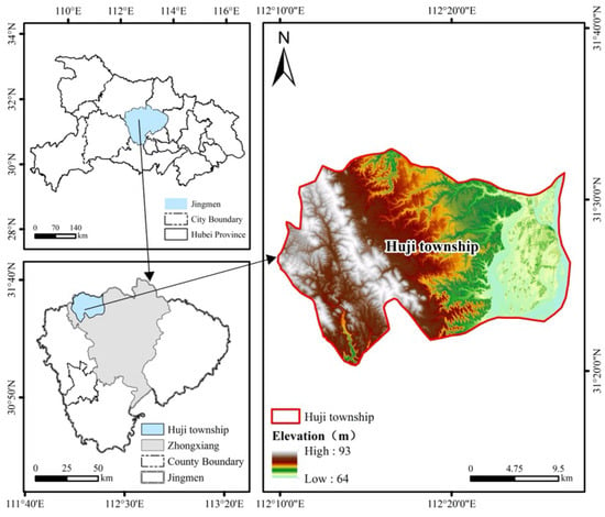
Figure 1. The geographical location of Lianhuashan.

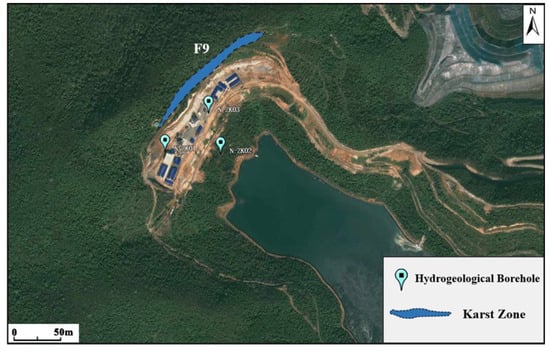
Figure 2. Location of pumping well.

2. Materials and Methods

2.1. Conceptual Model & Governing Equations

2.1.1. Conceptual Model

Based on the measured data of Lianhua Mountain, a simplified homogeneous aquifer model was built as a benchmark comparison model (baseline model). The model is a square area with a side length of 1000 m and a vertical thickness of 350 m. The boundary of the model is a constant head boundary. The model simulates an infinitely extended aquifer. The initial head is the annual average of the site measurement, which is 100 m. The pumping well is located in the center of the model, and the pumping flow is 1000 m³/d. The observation step is based on the pumping test specification. The conceptual model structure is shown in Figure 3. The initial parameter assignment of the model is shown in Table 1.

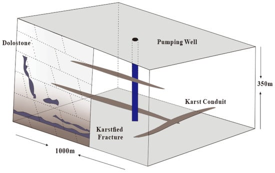
Figure 3. Conceptual model.

Table 1. Initial parameters.

Parameters	Horizontal Hydraulic Conductivity Kxy	Horizontal Hydraulic Conductivity Kz	Specific Storage S	Initial Head H
Value	0.8 m/d	0.08 m/d	0.08	100 m
Assignment basis	Field Pumping Tests	1/10 of Kxy	Field Pumping Tests	Average Head

The anisotropy ratio (Kz/Kxy = 0.1) is a common assumption in regional groundwater modeling of layered sedimentary or fractured-karst aquifers, reflecting the typical reduction in vertical permeability due to geological stratification. The constant-head boundary condition applied on all sides of the sufficiently large domain (1000 m × 1000 m) approximates an infinite aquifer for the duration of the simulated pumping test, a standard simplification that ensures the local drawdown is not artificially constrained by the boundary.

2.1.2. Governing Equations

Flow in the matrix is governed by Darcy’s law [15,16].

The governing equation is:

$$\begin{array}{c}{\displaystyle \frac{\mathsf{\partial }}{\mathsf{\partial }\mathrm{x}}}\left({\mathrm{K}}_{\mathrm{x}\mathrm{x}}{\displaystyle \frac{\mathsf{\partial }\mathrm{h}}{\mathsf{\partial }\mathrm{x}}}\right)+{\displaystyle \frac{\mathsf{\partial }}{\mathsf{\partial }\mathrm{y}}}\left({\mathrm{K}}_{\mathrm{y}\mathrm{y}}{\displaystyle \frac{\mathsf{\partial }\mathrm{h}}{\mathsf{\partial }\mathrm{y}}}\right)+\\ {\displaystyle \frac{\mathsf{\partial }}{\mathsf{\partial }\mathrm{z}}}\left({\mathrm{K}}_{\mathrm{z}\mathrm{z}}{\displaystyle \frac{\mathsf{\partial }\mathrm{h}}{\mathsf{\partial }\mathrm{z}}}\right)\pm \mathrm{W}=S_{\mathrm{s}}\left({\displaystyle \frac{\mathsf{\partial }\mathrm{h}}{\mathsf{\partial }\mathrm{t}}}\right)\end{array}$$

(1)

where ${\displaystyle \frac{\mathsf{\partial }}{\mathsf{\partial }\mathrm{x}}}$, ${\displaystyle \frac{\mathsf{\partial }}{\mathsf{\partial }\mathrm{y}}}$, ${\displaystyle \frac{\mathsf{\partial }}{\mathsf{\partial }\mathrm{z}}}$ denotes partial derivatives relative to the spatial coordinates X, Y, Z; K_xx, K_yy, K_zz represents the hydraulic conductivity components in the principal directions. h is the hydraulic head; Ss is the specific storage; W is the source/sink term (positive for a source, negative for a sink); ${\displaystyle \frac{\mathsf{\partial }\mathrm{h}}{\mathsf{\partial }\mathrm{t}}}$ denotes the temporal derivative of hydraulic head.

Karst conduits are discretized within the software. Flow in the conduits is governed by the Hagen–Poiseuille equation [17]:

$$\mathrm{Q}={\displaystyle \frac{\mathsf{\pi }{\mathrm{R}}^4\Delta \mathrm{p}}{8\mathrm{\mu L}}}$$

(2)

where Q is the flow rate, R is the conduit radius, Δp is the pressure drop along the conduit, μ is the fluid’s dynamic viscosity, and L is the conduit length.

Water exchange between the conduit and the matrix is driven by the hydraulic head gradient. Water flows from the conduit to the matrix when the conduit pressure is higher, and from the matrix to the conduit when it is lower [18]. This mass exchange is quantified by an exchange equation [19]:

$$\mathrm{Q}\mathrm{e}\mathrm{x}\mathrm{c}\mathrm{h}\mathrm{a}\mathrm{n}\mathrm{g}\mathrm{e} =\mathrm{K}\mathrm{m} \cdot \mathrm{A}\cdot \mathrm{b}(\mathrm{h}\mathrm{m} -\mathrm{h}\mathrm{p} )$$

(3)

where Km is the hydraulic conductivity of the matrix; A is the exchange surface area; hm and hp represent the hydraulic heads in the matrix and the conduit, respectively; b is the characteristic distance for exchange resistance.

2.2. Simulation Strategy and Inversion Workflow

As a finite element method-based groundwater modeling platform, FEFLOW (Finite Element subsurface FLOW system, version 7.0.1, DHI-WASY GmbH, Berlin, Germany) has unique advantages in characterizing heterogeneous flow systems in karst regions. The software provides multiple simulation approaches for handling heterogeneous flow, combined with 3D visualization and the PEST parameter inversion module, making it a powerful tool for studying karst groundwater system mechanisms [20,21].

This study adopted a “simulate-invert-compare” framework to assess the impact of karst conduits on the inversion of conventional hydrogeological parameters—a process referring to the estimation of aquifer properties (e.g., hydraulic conductivity, storativity) from observed field data such as drawdown during a pumping test. Synthetic “observed” data were generated from a model with prescribed parameters to mimic a field pumping test. This allowed for evaluating the accuracy of parameter inversion methods rooted in the homogeneity assumption.

The workflow comprises three steps (Figure 4): (1) Forward Simulation, where a heterogeneous model (Model-Real) generates synthetic drawdown data (${\mathrm{S}}_{\mathrm{o}\mathrm{b}\mathrm{s}}$); (2) Parameter Inversion, utilizing a homogeneous baseline model (Model-Base) and the PEST algorithm to derive equivalent hydraulic conductivity (${\mathrm{K}}_{\mathrm{i}\mathrm{n}\mathrm{v}}$) from ${\mathrm{S}}_{\mathrm{o}\mathrm{b}\mathrm{s}}$; and (3) Error Quantification, where the relative error ($\mathrm{R}\mathrm{E}$) is calculated by comparing ${\mathrm{K}}_{\mathrm{i}\mathrm{n}\mathrm{v}}$ against the true matrix conductivity (${\mathrm{K}}_{\mathrm{t}\mathrm{r}\mathrm{u}\mathrm{e}}$).

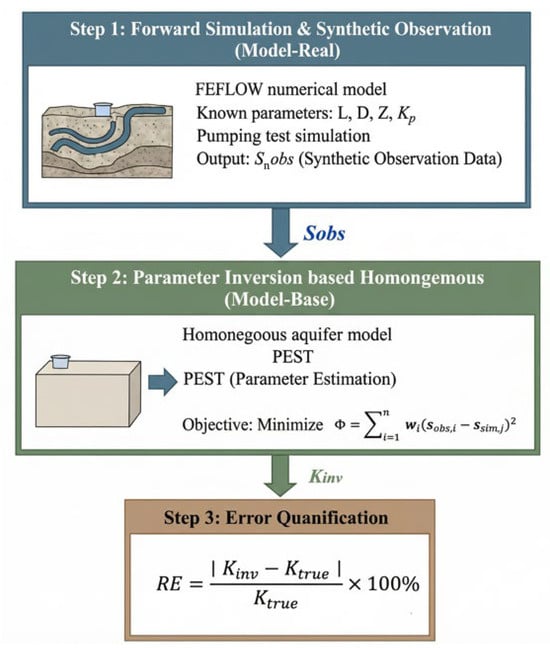
Figure 4. Research Approach.

2.2.1. Forward Simulation and Synthetic Observation

First, a reference model (Model-Real) incorporating conduits was developed in FEFLOW. Geometric parameters (length L, diameter D, depth Z) and hydraulic parameters (conduit hydraulic conductivity Kp) were specified for the conduits. A pumping well at the model center simulated a steady-state pumping test, and the temporal drawdown (S_obs) was recorded. This drawdown series is regarded as the synthetic “observed data” from a field pumping test.

2.2.2. Parameter Inversion Based on Homogeneous Assumption

A homogeneous aquifer model devoid of conduits was established as the “baseline model” (Model-Base), embodying the homogeneous simplification typically assumed in conventional hydrogeological surveys. The synthetic observation data (S_obs) from Model-Real were then used as the calibration target within the PEST (Parameter Estimation) module.

The inversion was performed using a nonlinear least squares optimization algorithm [22], which iteratively adjusted the equivalent hydraulic conductivity (K_inv) in Model-Base until the objective function (Φ), defined as the sum of squared residuals between the simulated (S_sim) and the synthetic drawdown observations, (S_obs), was minimized:

$$\mathsf{\Phi }={\sum }_{\mathrm{i}=1}^{\mathrm{n}}{\mathrm{w}}_{\mathrm{i}}({\mathrm{s}}_{\mathrm{o}\mathrm{b}\mathrm{s},\mathrm{i}}-{\mathrm{s}}_{\mathrm{s}\mathrm{i}\mathrm{m},\mathrm{i}}{)}^2$$

(4)

where n is the total number of observation points, and wi denotes the weighting factor. Upon convergence of Φ, the resulting K_inv is the inverted hydrogeological parameter under the given conduit conditions.

2.2.3. Error Quantification

To evaluate the accuracy of the inversion, the relative error (RE) is defined as a metric to quantify the parameter estimation bias induced by conduit presence:

$$\mathrm{R}\mathrm{E}={\displaystyle \frac{\mid {\mathrm{K}}_{\mathrm{i}\mathrm{n}\mathrm{v}}-{\mathrm{K}}_{\mathrm{t}\mathrm{r}\mathrm{u}\mathrm{e}}\mid }{{\mathrm{K}}_{\mathrm{t}\mathrm{r}\mathrm{u}\mathrm{e}}}}\times 100\%$$

(5)

where K_true is the matrix hydraulic conductivity (set at 0.8), and K_inv is the equivalent hydraulic conductivity obtained from the inversion. A larger RE indicates a greater deviation in parameter inversion caused by karst conduits.

2.3. Experimental Design for Sensitivity Analysis

To identify the key factors controlling inversion accuracy, a two-stage experimental approach was designed: single-variable conduit scenario simulations and Morris global sensitivity analysis.

2.3.1. Design of Conduit Scenarios

Based on karst hydrogeological characteristics and pumping test conditions, six influencing factors were selected and categorized into two groups:

Conduit Conditions: These parameters reflect the conduit’s geometry and hydraulics, including hydraulic conductivity (Kp), diameter (D), length (L), and burial depth (Z).

Pumping Conditions: These parameters represent the pumping rate and spatial configuration, encompassing the pumping rate (Q) and the distance between the well and the conduit (R).

The conduit models were constructed upon the baseline model, with the conduit simplified as regular cylindrical elements. Parameters such as conduit length, diameter, burial depth, hydraulic conductivity, and pumping rate can be adjusted as required for the study. (Figure 5).

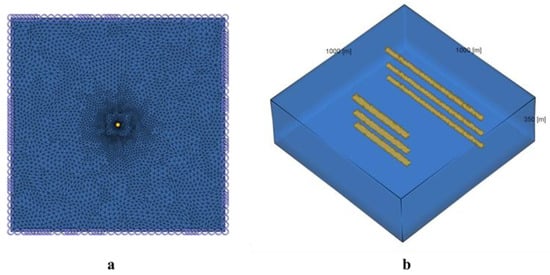
Figure 5. (a) 2D grid discretization, and (b) 3D conduit placemen.

2.3.2. Morris Sensitivity Analysis

The Morris method is a global sensitivity analysis technique that quantifies the influence of individual input parameters on a model output by computing averaged ‘Elementary Effects’ (EE) across multiple trajectories in the parameter space, effectively capturing parameter interactions and nonlinear effects [23]. To ensure that the sensitivity analysis covered a realistic and meaningful range, the levels for each factor (as listed in Table 2) were determined based on the field conditions of the Lianhuashan study area and typical value ranges for karst conduits reported in the literature. For example, the conduit hydraulic conductivity (Kp) spanned from lower than the matrix (0.1 m/d) to several orders of magnitude higher (100 m/d), representing scenarios from a clogged fissure to a well-developed underground river.

Table 2. Model design.

Category	Subcategory	Variation in Parameters	Number
Conduit Conditions	conductivity Kp (m/d)	0.1, 1, 10, 50, 100	5
	diameter D (m)	1.0, 2.0, 4.0, 6.0, 10.0	5
	length L (m)	50, 100, 200, 400, 600	5
	depth Z (m)	−50, −100, −150, −200, −250	5
Pumping Conditions	distance R (m)	0, 10, 25, 50, 100	5
	pumping rate Q (m3/d)	500, 750, 1000, 1250,1500	5
Sensitivity		24	24
Total			54

For the sensitivity analysis, a total of 24 parameter sample sets were generated using a structured, one-at-a-time (OAT) sampling design based on the Morris method. This design creates multiple trajectories in the parameter space, where each trajectory varies one parameter at a time across its pre-defined levels while holding others fixed. The 24 sets represent the outcomes of these guided trajectories, ensuring that the elementary effects for each parameter are calculated across a representative subset of the full factorial design. This approach provides a robust and computationally efficient screening of parameter sensitivities.

The assessment was based on two metrics: the mean absolute value of the elementary effects (μ*) and their standard deviation (σ):

(μ*): The mean absolute Elementary Effect, quantifying the overall influence of a parameter on the inversion error. A higher μ* denotes greater parameter sensitivity.

σ: The standard deviation of the Elementary Effects, reflecting the degree of interaction with other parameters or nonlinearity in its effect. A larger σ implies the parameter’s impact is less stable and more dependent on the values of other parameters.

Based on the research objectives outlined above, 54 models were constructed (Table 2).

3. Results

The results are presented in the sequence of “flow field pattern—drawdown curve—equivalent parameters and error”.

3.1. Impact of Conduit Conditions (Kp, D, L, Z)

3.1.1. Flow Field Patterns

As the conduit hydraulic conductivity increases, the equipotential lines evolve from circular to elongated ellipses along the conduit axis, and the cone of depression is lengthened (Figure 6a). When Kp approaches the matrix value (approximately 1 m/d), the flow field resembles that of the baseline model, showing good symmetry (Figure 6a).

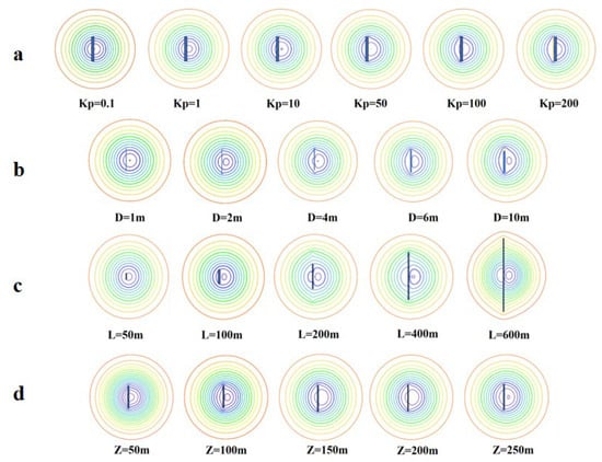
Figure 6. Groundwater flow fields under different conduit conditions. (a) Groundwater flow field under different conduits conductivity (b) Groundwater flow field under different conduits diameter (c) Groundwater flow field under different conduits length (d) Groundwater flow field under different conduits depth.

Increasing the conduit diameter amplifies the flow field deformation. As the diameter increased from 1 m to 10 m, the distortion and elongation of the cone of depression along the conduit axis progressively intensified (Figure 6b).

For short conduits with lengths (L) less than the radius of pumping influence (L ≤ 200 m), the entire conduit lay within the cone of depression, resulting in minimal alteration to the overall flow field (Figure 6c). In contrast, when the conduit length extended to intermediate or distal zones (L ≥ 200 m), it transmitted water from beyond the influence radius to the well, significantly modifying the cone of depression. This caused the equipotential lines to become skewed and elongated along the conduit’s path (Figure 6c).

The influence of the conduit burial depth (Z) on the flow field manifested primarily in the vertical dimension, causing only minor alterations to the flow pattern near the pumping well. Contours of equal head were moderately skewed along the conduit’s axial direction, a feature that remained largely unchanged with increasing burial depth (Figure 6d).

3.1.2. Drawdown Curve

For models with different conduit hydraulic conductivities: In the early pumping phase (Figure 7a), the model featuring a low-conductivity conduit (Kp = 0.1 m/d) displayed the maximum drawdown at the well. The drawdown curves from other models were virtually identical to the baseline model’s curve. As pumping continued into the mid-to-late phase (Figure 7b), the final drawdown amplitude diminished with increasing conduit conductivity. During the recovery phase (Figure 7c), high-conductivity conduits facilitated a more rapid water level recovery.

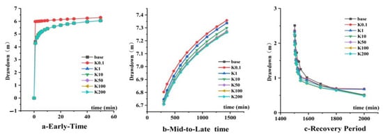
Figure 7. Drawdown–time curves for different conduit hydraulic conductivity.

Drawdown–time curves for models with varying conduit diameters showed consistent behavior. During the mid-to-late pumping stages (Figure 8a,b), all curves for pipes containing conduit remained above baseline. Larger conduit diameters resulted in smaller drawdown and faster water recovery (Figure 8c).

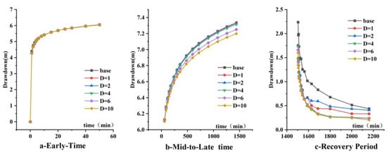
Figure 8. Drawdown–time curves for different conduit diameter (D).

The drawdown curves diverged significantly with conduit length. For short conduits (L ≤ 200 m), the drawdown exceeded that of the baseline model during the mid-to-late pumping phases (Figure 9b). In contrast, models with long conduits (L ≥ 200 m) consistently exhibited lower drawdown than the baseline (Figure 9a,b). During recovery, a longer conduit length correlates with a more rapid water level rebound (Figure 9c).

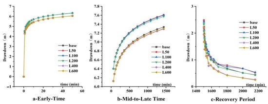
Figure 9. Drawdown–time curves for different conduit length (L).

Drawdown curves for models with different conduit burial depths showed minor differences: during both pumping and recovery, the curves ran parallel and were all slightly above the baseline. The shallow-burial model showed slightly faster recovery early on, but all curves converged later (Figure 10).

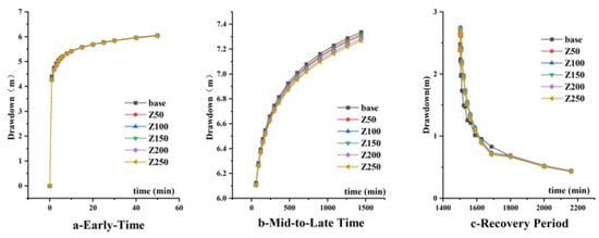
Figure 10. Drawdown–time curves for different conduit burial depths (Z).

3.1.3. Equivalent Hydraulic Conductivity and Inversion Error

The inversion error (RE) displayed a pattern of initial decrease, followed by an increase, and eventual leveling off with rising conduit hydraulic conductivity (Kp). The error reached its minimum (1.87%) when Kp approximated the matrix value (~1 m/d). For a low Kp (0.1 m/d), Kinv was underestimated (RE ≈ 14.15%). When Kp ≥ 10 m/d, Kinv was overestimated, and the magnitude of overestimation plateaued (Figure 11a).

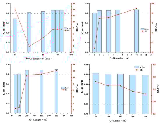
Figure 11. Parameter inversion results and errors for different conduit conditions.

The inversion error (RE) shows a monotonic increase with conduit diameter. Furthermore, the estimated Kinv for all scenarios exceeded the baseline value of 0.8 m/d (Figure 11b).

The inversion error (RE) remained very small (<1%) for conduit lengths (L) less than 200 m. Beyond this length, RE increased from about 1% to approximately 11%, showing a gradual rise with increasing L (Figure 11c).

The RE decreased slightly as the conduit burial depth Z increased (from ~7.75% to ~7.31%), with minimal variation (Figure 11d).

3.2. Integrated Effects of Pumping Conditions (Q, R)

3.2.1. Flow Field and Drawdown Responses

Varying the pumping rate mainly alters the intensity of the pumping disturbance and its radius of influence. This amplifies the flow field asymmetry, but the fundamental flow pattern is preserved (Figure 12a). While a higher pumping rate yields greater drawdown magnitude, the temporal shape of the drawdown curve is largely unchanged (Figure 13a). Recovery is slower for models subjected to higher pumping rates (Figure 13b).

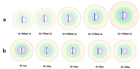
Figure 12. Flow fields under different pumping conditions. (a) Groundwater flow field under different pumping rate; (b) Groundwater flow field under different distance.

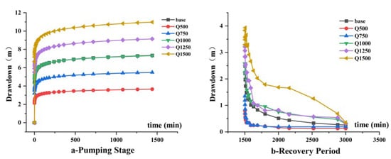
Figure 13. Drawdown–time curves for different pumping rates.

The distance (R) between the pumping well and the conduit is the primary factor altering the flow field near the well. When R = 0 m, the cone of depression is strongly elongated along the conduit direction. Noticeable distortion was still observed at R = 10–25 m, while the contours of equal head became nearly symmetrical for R ≥ 50 m (Figure 12b). The simulated drawdown increased with greater well-conduit distance, causing the drawdown curves to converge towards the baseline model’s curve (Figure 14a).

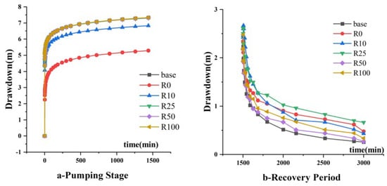
Figure 14. Drawdown–time curves for different well-conduit distances.

Furthermore, models with smaller well-conduit distances exhibited significantly faster water recovery (Figure 14b).

3.2.2. Equivalent Hydraulic Conductivity and Inversion Error

The inversion error (RE) exhibited limited fluctuation with pumping rate. It peaked (approximately 10.29%) at a pumping rate (Q) of 500 m³/d, subsequently declining and stabilizing within a narrow range of ~8.55–8.99% for Q between 750 and 1500 m³/d (Figure 15a).

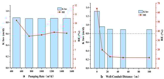
Figure 15. Parameter inversion results and errors for different pumping conditions.

The inverted hydraulic conductivity (Kinv) decreased with greater well-conduit distance (R). Correspondingly, the relative error (RE) declined sharply from 64.22% to 12.37% as R increased from 0 to 25 m, and plateaued at approximately 11.4% for R ≥ 50 m (Figure 15b).

4. Discussion

4.1. Interpretation of Sensitivity Analysis

The parameter inversion results (K_inv) and associated errors (RE) from the 24 sensitivity model runs conducted for the Morris analysis are summarized in Table 3. These results serve as the direct input for the subsequent computation of the sensitivity metrics (elementary effects). The calculated mean (μ*) and standard deviation (σ) of these effects for each parameter are presented and analyzed below.

Table 3. Sensitivity model inversion results.

Model	Kp	D	L	Z	R	Q	Kinv	RE%
1	0.1	1	600	50	0	500	0.722283	9.71%
2	100	1	600	50	0	500	0.960124	20.02%
3	100	6	600	50	0	500	1.288864	61.11%
4	100	6	50	50	0	500	0.903151	12.89%
5	100	6	50	250	0	500	0.90385	12.98%
6	100	6	50	250	100	500	0.8032	0.40%
7	1	1	100	100	10	750	0.822199	2.77%
8	100	1	100	100	10	750	0.89238	11.55%
9	100	6	100	100	10	750	0.861616	7.70%
10	100	6	600	100	10	750	0.886274	10.78%
11	100	6	600	250	10	750	0.883179	10.40%
12	100	1	600	250	10	750	0.876075	9.51%
13	10	2	200	150	25	1000	0.814129	1.77%
14	100	2	200	150	25	1000	0.897702	12.21%
15	100	6	200	150	25	1000	0.898773	12.35%
16	100	6	50	150	25	1000	0.81737	2.17%
17	100	6	50	250	25	1000	0.817895	2.24%
18	100	2	50	250	25	1000	0.815117	1.89%
19	50	4	400	200	50	1250	0.82569	3.21%
20	100	4	400	200	50	1250	0.857325	7.17%
21	100	6	400	200	50	1250	0.87978	9.97%
22	100	6	50	200	50	1250	0.817978	2.25%
23	100	4	50	50	50	1250	0.81364	1.71%
24	50	4	50	50	50	1250	0.802564	0.32%

The mean (μ*) and standard deviation (σ) of the elementary effects were calculated for the sensitivity models. Comparing μ*and σ facilitated the identification of primary controlling factors and secondary factors responsible for parameter inversion errors (Table 4).

Table 4. Morris Sensitivity Analysis Results.

Factors	(μ*)	(σ)	Ranking
Well-Conduit Distance (R)	0.352	0.285	1
Length (L)	0.128	0.095	2
Conductivity (Kp)	0.103	0.078	3
Diameter (D)	0.087	0.064	4
Pumping Rate (Q)	0.025	0.018	5
Burial Depth (Z)	0.008	0.006	6

The well-conduit distance (R) ranked as the most sensitive parameter, with its mean elementary effect (μ* = 0.352) significantly higher than others. Its standard deviation (σ = 0.285) was also the largest. It exhibited interaction with other parameters and was the most critical factor contributing to inversion errors. Conduit length (L), hydraulic conductivity (Kp), and diameter (D) followed in sensitivity (second, third, and fourth, respectively). Their σ/μ* ratios were all below 1, indicating relatively stable linearity. In contrast, pumping rate (Q) and pipeline burial depth (Z) were relatively insensitive factors.

4.1.1. The Controlling Role of Spatial Configuration (R)

The distance between the well and the conduit (R) emerged as the most sensitive parameter. This stems from the extreme heterogeneity inherent to karst aquifer flow fields, where hydraulic deformation is predominantly localized around the conduit. At minimal distances (R ≈ 0), direct hydraulic connection places conduit flow as the dominant source of well replenishment, substantially reducing observed drawdown and resulting in significant inversion error (RE = 64.22% at R = 0 m, Figure 15b). As the distance increases beyond a certain range (R > 50 m), matrix flow regains dominance, and the inversion error decreases sharply—a phenomenon that accounts for the markedly different hydraulic conductivity values obtained from closely spaced boreholes in field studies like those at Lianhua Mountain. The conduit’s impact on inversion results asymptotically approaches a constant level once the well-conduit distance surpasses a critical value related to the radius of pumping influence.

4.1.2. Influence of Conduit Recharge Capacity (L, D, Kp)

The conduit length (L), diameter (D), and hydraulic conductivity (Kp) of a conduit govern its recharge capacity by controlling the “ catchment area”, the “cross-sectional area for flow”, and the “transmissivity”, respectively. Higher values for these parameters strengthen the conduit’s ability to convey water to the well, leading to reduced drawdown and a greater degree of overestimation in the inverted hydraulic conductivity. Moreover, the impact of conduit length (L) on inversion error plateaus beyond a certain threshold (Figure 14), suggesting that the marginal benefit of additional recharge from distal conduit segments diminishes due to increasing frictional head losses along the conduit.

4.1.3. Insensitive Factors (Q, Z)

The pumping rate (Q), governing the stress intensity on the aquifer, alters the magnitude of drawdown but does not modify the fundamental flow geometry dictated by the conduit network (Figure 12a). Therefore, the relative error (RE) shows minimal sensitivity to Q. The conduit burial depth (Z), controlling only the vertical position, leads to a very slight decrease in RE with greater depth (Figure 11d). This occurs because increased depth prolongs the hydraulic response time from the conduit, elevating the proportion of matrix flow contribution during the test. This shifts the system response closer to that of the true matrix parameters. Over the duration of a typical test, the total conduit discharge remains effectively unchanged, leading to convergent drawdown curves and resulting in only minor changes to the inversion error.

4.2. Physical Mechanism of Inversion Error

Parameter inversion in conventional pumping test analysis assumes a homogeneous aquifer, resulting in a symmetrical cone of depression and a drawdown–time curve that follows the standard Theis solution. In karst terrains, however, karst conduits act as “virtual recharge boundaries” during pumping, significantly altering the flow field pattern, the drawdown response, and consequently, the parameter estimation [3]:

4.2.1. Flow Field Distortion

Acting as a preferential flow path due to its high conductivity, the karst conduit locally reduces the hydraulic gradient in its vicinity. This redirects streamlines from a concentric pattern towards the conduit itself. Enhancing the conduit’s transmissive properties—by increasing its hydraulic conductivity (Kp), length (L), or diameter (D)—intensifies and expands the resulting flow field distortion (Figure 6). Conversely, the insensitive factors—conduit burial depth (Z) and pumping rate (Q)—affect the timing of the conduit’s response and the stress magnitude but do not reshape the fundamental flow pattern established by the conduit’s conductivity.

4.2.2. Drawdown Attenuation

During pumping, conduits attenuate drawdown by rapidly releasing their stored water and efficiently transmitting groundwater from remote regions to the well. This additional recharge is reflected in the drawdown–time curves as a slower rate of decline. Consequently, throughout the pumping test, the simulated drawdown for all models containing conduits was less than that of the baseline model (their curves are plotted above the baseline curve). This enhanced recharge also led to a more rapid water level recovery after pumping ceases. The overall shape of the drawdown and recovery curves resembles the response expected from a constant-head boundary or a leaky aquifer.

4.2.3. Erroneous Compensation in Parameter Inversion

The inversion process thus compensates erroneously when homogeneous-assumption-based algorithms (PEST) are applied to fit the attenuated drawdown data. Unable to discern the discrete conduit structure, these algorithms can only replicate the reduced drawdown by elevating the effective hydraulic conductivity of the entire model domain. The resulting inverted conductivity represents a composite average of the low-permeability matrix and the high-permeability conduit, incorporating a significantly overestimated component from the latter. This value inevitably exceeds the true matrix conductivity, introducing bias into subsequent predictions.

4.2.4. Case Demonstration

A concrete example vividly illustrates the integrated physical mechanism. Model R1 (with a high-conductivity conduit: Kp = 100 m/d, D = 2 m, L = 200 m, placed directly at the well, R = 0 m) exhibited the most severe flow field distortion, where the cone of depression was intensely elongated along the conduit axis (Figure 12b for R = 0). This preferential flow path acts as a virtual recharge boundary, drastically attenuating drawdown at the well—its drawdown–time curve lies significantly above the baseline (Figure 14a). When the homogeneous-assumption inversion algorithm (PEST) is forced to fit this attenuated drawdown response, it cannot attribute the reduced drawdown to a local discrete feature. Instead, it erroneously compensates by elevating the equivalent hydraulic conductivity of the entire model domain, resulting in a severely overestimated Kinv of 1.314 m/d and a large relative error (RE) of 64.22% (see the attached schedule). This case clearly links the sequence: conduit proximity → flow field distortion → drawdown attenuation → overestimation of inverted conductivity.

4.3. Outlook

4.3.1. From Single Conduit to Conduit Networks

While this study elucidated how karst conduits distort parameter inversion from conventional pumping tests, enhancing the mechanistic understanding of complex karst flow fields, the models are still predicated on a single, simplified conduit. Real karst aquifers typically consist of intricate, interconnected conduit networks. Future research should therefore progress towards simulating complex three-dimensional networks to better address practical engineering needs. This entails developing 3D stochastic network models incorporating multi-branched and intersecting conduits. A systematic investigation into how network properties—such as branching degree, connectivity, conduit diameter distribution, and well-network spatial configuration—affect drawdown responses and bias in equivalent parameter estimation would yield more realistic simulations. Furthermore, integrating numerical experimentation with theoretical upscaling approaches could establish parameter transfer functions across scales (well-test to site to region), clarifying the applicability limits of dual-permeability versus discrete conduit models under varying network densities and connectivity patterns.

4.3.2. Parameter Correction and Spatial Conduit Characterization

Forward simulations elucidate the error mechanisms, yet the inverse problem—extracting true matrix parameters and inferring conduit geometry from distorted field data—is critical for translating mechanistic insights into practical applications. Future efforts should focus on developing a physics-informed data fusion framework. Integrating multi-source observations (e.g., drawdown, tracers, temperature/electrical conductivity, and hydrogeophysical surveys) can mitigate the limitations of single-method approaches. Comparative analysis and model selection among equivalent porous medium, dual-permeability, and discrete conduit models will be necessary to match site-specific karst heterogeneity.

For practical implementation, merging physical principles with machine learning techniques (such as deep learning and Bayesian inversion) holds promise for creating advanced interpretation tools. These tools could automate the identification of conduit signatures within pumping test data while concurrently correcting hydrological parameters. Establishing a reproducible, model-driven workflow would significantly enhance the interpretation of field pumping tests, improve parameter estimation, and optimize wellfield design.

5. Conclusions

To address the challenge that strong heterogeneity posed by karst conduits brings to the inversion of hydrogeological parameters from pumping tests, this study employed a numerical simulation approach. A ‘simulate-invert-compare’ framework based on FEFLOW was established to quantify the impact of various conduit characteristics and pumping conditions on parameter estimation errors. The main findings are as follows:

• The existence of karst conduits alters groundwater recharge pathways and flow field morphology, causing depression cones to elongate along the conduit axis and exhibit asymmetry. This manifests on drawdown curves as reduced water level drawdown and accelerated recovery rates in observation wells. As a result, conventional inversion techniques that assume homogeneity overestimate the equivalent hydraulic conductivity.
• The distance between the pumping well and the conduit (R) is the primary factor influencing inversion error. The error sharply declines with increasing R: When R < 25 m, the conduit serves as a direct pathway to the well and the homogeneous inversion method fails, resulting in substantial inversion error. For R > 50 m, the conduit progressively moves beyond the influence of the precipitation funnel, leading to the stabilization of inversion errors.
• The relative magnitude of the conduit hydraulic conductivity (Kp) to the matrix conductivity determines the direction of inversion error deviation. When the conduit permeability coefficient is lower than the matrix, the conduit acts as a relatively impermeable boundary, leading to the underestimation of inversion values. Conversely, when the conduit permeability coefficient exceeds that of the matrix, increased conduit flow recharge causes the overestimation of inversion values.
• The length of karst conduits (L) determines the catchment area, while conduit diameter (D) dictates the cross-sectional flow area. Both parameters exhibit a positive correlation with inversion error, such that longer and larger conduits lead to greater parameter overestimation. Furthermore, conduit length exhibits a critical threshold beyond which its influence on error diminishes progressively.
• Conduit burial depth (Z) and pumping rate (Q) are low-sensitivity factors. Variations in pumping rate affect the drawdown magnitude but do not change the drawdown response pattern dictated by the conduit network. Similarly, burial depth controls the vertical conduit location, leaving the total recharge contribution largely unchanged. Both factors exert limited influence on inversion errors.

References

- Niemann, W.L.; Rovey, C.W., II. A systematic field-based testing program of hydraulic conductivity and dispersivity over a range in scale. Hydrogeol. J. 2008, 17, 307–320. [Google Scholar] [CrossRef]
- Theis, C.V. The relation between the lowering of the Piezometric surface and the rate and duration of discharge of a well using ground-water storage. Eos Trans. Am. Geophys. Union 2014, 16, 519–524. [Google Scholar] [CrossRef]
- Xu, Z.; Zhou, X.; Cui, X.; Tuo, M.; Wang, X.; Zhang, Y. Advances in Groundwater Numerical Modelling in Karst Regions. Chin. Karst 2018, 37, 475–483. [Google Scholar] [CrossRef]
- Qin, F.; Zhan, S.; Zheng, X.; Chen, Y.; Du, X.; Yang, Z. Quantitative assessment of tunnel construction and persistent drought on karst groundwater. China Rural Water Hydropower 2024, 137–146. Available online: https://kns.cnki.net/kcms2/article/abstract?v=4qE7rfs4XRFdgIzzYpd8Lvg-QcfimICeEgf7W9Ig3Zo-hBbVlKAWCnr2RtF1J1YFIw6m_CL0f0sLhVO4uoVGIjzHK5mPyMZxVCMxPNZPKrFvUYZ09onuCLJk9gHNOVXGOeWfP3m0p4c532IcpBUPjEuDimkgkbDuUWBkuZY3Re5YpXon_5dUyr67QnE6ZpN_&uniplatform=NZKPT&language=CHS (accessed on 15 April 2025).
- Yang, Y.; Tang, J.; Su, C.; Pan, X.; Zhao, L. Research progress on multi-medium water flow models in karst regions. Chin. Karst 2014, 33, 419–424. Available online: https://kns.cnki.net/kcms2/article/abstract?v=4qE7rfs4XREsFn3ngIoSiQzyTkYLHd-rec6xz2mZwxPCXCMYRLjC7fNUwQtYUUZPyHqkosVrQMHbJ0jczfG8LovRzxWUf0yI1kThwdK8LBwPaxQ4_mxkxfJW6qdBaiiTfpfS4M5xuWw-kqWK9TNuRHpiRIYsFx-85QVR_tpqlfuKy5UlYS_DyQeF1RFSwXLd&uniplatform=NZKPT&language=CHS (accessed on 22 July 2025).
- Gao, Y.; Xu, Z.; Li, S.; Yu, W. Modeling Monthly Nitrate Concentration in a Karst Spring with and without Discrete Conduit Flow. Water 2022, 14, 1622. [Google Scholar] [CrossRef]
- Tang, Y. Multiscale Numerical Simulation of the Kunming-Chengdu Tunnel’s Karst Pipeline Crossing the Black and White Dragon Pools in the Central Yunnan Water Diversion Project. Master’s Thesis, Chengdu University of Technology, Chengdu, China, 2018. [Google Scholar]
- Zhao, L.; Xia, R.; Yang, Y.; Shao, J.; Cao, J.; Fan, L. Numerical simulation of karst conduit flow based on the CFP method: A case study of the Zhaidi Underground River subsystem in Guilin. Acta Geol. Sin. 2018, 39, 225–232. Available online: https://link.cnki.net/urlid/11.3474.P.20171125.1733.004 (accessed on 5 September 2025).
- Robineau, T.; Tognelli, A.; Goblet, P.; Renard, F.; Schaper, L. A double medium approach to simulate groundwater level variations in a fissured karst aquifer. J. Hydrol. 2018, 565, 861–875. [Google Scholar] [CrossRef]
- Xiang, Z.; Yu, S.; Wang, X. Modeling the Hydraulic Fracturing Processes in Shale Formations Using a Meshless Method. Water 2024, 16, 1855. [Google Scholar] [CrossRef]
- Huang, L.; Liang, J.; Zhu, J.; Yang, P.; Li, T. Laboratory Study on the Characteristics of Groundwater Level Variations in Pipe-Fissure Karst Systems. J. Guizhou Univ. (Nat. Sci. Ed.) 2024, 41, 41–48. [Google Scholar] [CrossRef]
- Wang, J.; Li, S.; Li, L.; Xu, Z. Dynamic Evolution Characteristics of Tunnel Karst Pipeline-Type Water Inrushes and Comprehensive Prediction of Water Inrush Volume. Chin. J. Geotech. Eng. 2018, 40, 1880–1888. Available online: https://link.cnki.net/urlid/32.1124.TU.20180116.0925.012 (accessed on 29 September 2025).
- Xu, S.; Yu, Y.; Liao, P.; Cai, Z.; Liu, J.; Chen, Y. Identification of karst recharge sources for the main shaft at the Lianhuashan section of the Jingxiang phosphate mine in Hubei Province. Hydrogeol. Eng. Geol. 2025, 52, 109–120. Available online: https://link.cnki.net/doi/10.16030/j.cnki.issn.1000-3665.202502032 (accessed on 18 October 2025).
- Liang, C.; Chen, Z.; Li, W.; Yi, C.; Jiang, Y.; Song, Y.; Wang, X.; Wang, Y. Application of Tracer Tests in Investigating Groundwater Pollution at Metal Mines in Karst Regions. J. Land Resour. 2024, 21, 43–47. Available online: https://link.cnki.net/doi/10.20147/j.cnki.gtzydk.2024.03.006 (accessed on 4 November 2025).
- Wu, J. Groundwater Hydrodynamics; China Water & Power Press: Beijing, China, 2009. [Google Scholar]
- Hubbert, M.K. The Theory of Ground-Water Motion. J. Geol. 1940, 48, 785–944. [Google Scholar] [CrossRef]
- Liu, J.; Xu, G.; Ma, X. A Discussion on the Construction Method of Karst Pipeline Models Based on FEFLOW. Chin. Karst 2015, 34, 586–590. Available online: https://kns.cnki.net/kcms2/article/abstract?v=4qE7rfs4XRFrwYdDmnCvgHYirlgmpTdXKk64plFQSB-OtN2vXKsoy6hK6dI8e_NAQq_cDPunWNRipgXVzEP5QEUxj4Mw61q3nXEXFJz3Z9Q1J2jZjD4J83i6Gj090ANq48o3laQgRvQN3qaHrXr-BZgpPrt7cETK80Q02CPH3wxuVvQGPyCVBy1fb6MTEEUU&uniplatform=NZKPT&language=CHS (accessed on 5 November 2025).
- Warren, J.E.; Root, P.J. The Behavior of Naturally Fractured Reservoirs. Soc. Pet. Eng. J. 1963, 3, 245–255. [Google Scholar] [CrossRef]
- Luo, M.; Chen, J.; Ji, H.; Wan, L.; Li, C.; Zhou, H. Advances in the Study of Solute Exchange between Karst Pipes and Fractured Media. Earth Sci. 2023, 48, 4202–4213. Available online: https://link.cnki.net/urlid/42.1874.P.20220119.1649.008 (accessed on 7 November 2025).
- Gao, H.; Yang, M.; Hei, L.; Ye, C. Application of MODFLOW and FEFLOW in Groundwater Numerical Modelling in China. Groundwater 2012, 34, 13–15. Available online: https://kns.cnki.net/kcms2/article/abstract?v=VUvWpoE9A3Lv8rdUITKznv-otZIVKMleM2T6BK-VDfegTZZIo9Hif-fVLHG2qdTpiSY_MMN0BrSJGAV6B6mXbfOKumHPJrAjK7-AB8qrd210YDQq6ZLd9Cl0YMHWpMl5lR6tnHI7QT6oExTXrwKKjR_26JuYcGaIP-okbrELxcAnwVKdD7ozmA==&uniplatform=NZKPT&language=CHS (accessed on 13 November 2025).
- Hu, J.; Zhang, X.; Wei, Z. A Review of FEFLOW Applications in Groundwater Numerical Modelling. Groundwater 2020, 42, 9–13. [Google Scholar] [CrossRef]
- Phelan, D.J.; Miller, C.V. Occurrence and Distribution of Organic Wastewater Compounds in Rock Creek Park, Washington, D.C., 2007–2008; US Geological Survey: Reston, VA, USA, 2010. [CrossRef]
- Campolongo, F.; Cariboni, J.; Saltelli, A. An effective screening design for sensitivity analysis of large models. Environ. Model. Softw. 2007, 22, 1509–1518. [Google Scholar] [CrossRef]
Disclaimer/Publisher’s Note: The statements, opinions and data contained in all publications are solely those of the individual author(s) and contributor(s) and not of MDPI and/or the editor(s). MDPI and/or the editor(s) disclaim responsibility for any injury to people or property resulting from any ideas, methods, instructions or products referred to in the content. |
© 2026 by the authors. Licensee MDPI, Basel, Switzerland. This article is an open access article distributed under the terms and conditions of the Creative Commons Attribution (CC BY) license.