Season-Aware Ensemble Forecasting with Improved Arctic Puffin Optimization for Robust Daily Runoff Prediction Across Multiple Climate Zones

Abstract

Accurate daily runoff forecasting is essential for flood control and water resource management, yet existing models struggle with the seasonal non-stationarity and inter-basin variability of runoff sequences. This paper proposes a Season-Aware Ensemble Forecasting (SAEF) method that integrates SVM, LSSVM, LSTM, and BiLSTM models to leverage their complementary strengths in capturing nonlinear and non-stationary hydrological dynamics. SAEF employs a seasonal segmentation mechanism to divide annual runoff data into four seasons (spring, summer, autumn, winter), enhancing model responsiveness to seasonal hydrological drivers. An Improved Arctic Puffin Optimization (IAPO) algorithm optimizes the model weights, improving prediction accuracy. Beyond numerical gains, the framework also reflects seasonal runoff generation processes—such as rapid rainfall–runoff in wet seasons and baseflow contributions in dry periods—providing a physically interpretable perspective on runoff dynamics. The effectiveness of SAEF was validated through case studies in the Dongjiang Hydrological Station (China), the Elbe River (Germany), and the Quinebaug River basin (USA), using four performance metrics (MAE, RMSE, NSEC, KGE). Results indicate that SAEF achieves average Nash–Sutcliffe Efficiency Coefficient (NSEC) and Kling–Gupta efficiency (KGE) coefficients of over 0.92, and 0.90, respectively, significantly outperforming individual models (SVM, LSSVM, LSTM, BiLSTM) with RMSE reductions of up to 58.54%, 55.62%, 51.99%, and 48.14%. Overall, SAEF not only strengthens predictive accuracy across diverse climates but also advances hydrological understanding by linking data-driven ensembles with seasonal process mechanisms, thereby contributing a robust and interpretable tool for runoff forecasting.

1. Introduction

Runoff is a key component of the hydrological cycle. Accurate runoff forecasting is essential for flood mitigation, water resources management, and ecological protection. Influenced by seasonal rainfall, human activities, and solar radiation, runoff shows marked nonlinearity, multi-scale variability, and spatio-temporal non-stationarity, which together increase modeling uncertainty [1]. These traits make runoff forecasting more challenging, motivating researchers to develop more robust and accurate modeling approaches. Therefore, developing integrated models that recognize seasonal differences and dynamically adapt forecasting strategies can both deepen our understanding of complex hydrological processes and better support flood control, disaster mitigation, and water-resource allocation.

1.1. Methodology Review and Current Challenges

Over the past few decades, a large number of runoff forecasting methods have been successfully developed. These methods can be classified into four main categories: statistical models [2], physical models [3], machine learning (ML) models [4], and deep learning (DL) models [5,6,7,8]. Traditional physical models are built on hydrological cycle principles and multi-source data (e.g., terrain and soil) [9]. Examples include TOPMODEL [10] and SWAT [11], which offer clear physical interpretability. However, these models typically require many parameters, have complex structures, and depend on high-quality input data, which limits their adaptability to nonlinear and non-stationary runoff dynamics [12]. Statistical models rely on the statistical characteristics of historical data for forecasting [13,14], such as autoregressive and Kalman filtering methods. Although these methods simplify the calculation process, they are unable to effectively capture the nonlinear relationships in the runoff process, resulting in limited model forecasting accuracy. Therefore, maintaining model robustness under seasonally varying hydrological conditions has become a critical issue in data-driven runoff forecasting.

In recent years, the rapid development of artificial intelligence has promoted the widespread application of ML and DL in the field of runoff forecasting, making them the main methods in this field. Initially, technologies such as support vector machines (SVMs) and long short-term memory networks (LSTMs) were widely used in runoff forecasting [15,16,17]. Subsequently, these technologies have continued to evolve, giving rise to more advanced models. For example, least squares support vector machines (LSSVMs), as an improved version of SVM, significantly reduce computational complexity by converting quadratic programming problems into linear equation systems. At the same time, LSSVM uses a least squares loss function to further improve its efficiency and robustness in large-scale runoff forecasting tasks [18,19]. Compared to traditional SVM, LSSVM inherits its advantages while reducing reliance on assumptions about data distribution, demonstrating stronger generalization capabilities [20,21]. Xu et al. [18] applied the LSSVM to monthly runoff forecasting. The forecasting performance was significantly superior to that of the SVM, effectively improving the forecasting accuracy of complex runoff sequences and the ability to capture extreme values. Meanwhile, the bidirectional long short-term memory network (BiLSTM), as an extension of LSTM, enhances modeling capabilities for context dependencies by simultaneously capturing forward and backward information in sequence data, thereby significantly improving the accuracy and robustness of sequence data processing. BiLSTM retains the advantages of the LSTM memory gate structure while effectively overcoming the limitations of unidirectional information flow, making it more suitable for complex time series forecasting tasks [22,23]. Table 1 systematically summarizes the core characteristics of and application differences in several mainstream runoff forecasting models. Therefore, maintaining model robustness under seasonally varying hydrological conditions has become a critical issue in data-driven runoff forecasting.

Table 1. Summary of methods and core conclusions of different models in hydrological prediction.

Author	Method	Conclusions
Shahnazi, et al. [24]	For groundwater drought forecasting, this study monitors drought with SGI, decomposes sequences via CEEMDAN, VMD, and other preprocessing, and builds a GWO-optimized SVM hybrid model for multi-term prediction.	Using the technical route of “preprocessing decomposition-optimized prediction-clustering verification”, this study improves groundwater drought prediction accuracy, with the VMD-GWO-SVM model performing best, providing a scientific method for semi-arid area drought early warning.
Chang, et al. [25]	For medium and long-term runoff prediction of Lianghekou Hydrological Station, this study constructs P-XGBoost-SHAP framework, focuses on building LSTM, SVM, and other data-driven models, and optimizes results with EEMD-AR.	After EEMD-AR correction, models like LSTM and SVM achieve NSE of ~0.93 in validation, with significantly improved accuracy. SHAP clarifies core driving mechanisms, supporting basin water resource optimization.
Hu, et al. [26]	For monthly runoff prediction in arid alpine basins of NW China, taking the Qarqan River Basin as the study area, EMD decomposition and PCA dimensionality reduction are used to build an EMD-PCA-LSTM model for comparison with other LSTM models.	Using the coupled method of “EMD decomposition-PCA dimensionality reduction-LSTM prediction”, the model effectively captures runoff characteristics with superior accuracy, supporting basin water resource management and drought-flood early warning.
An et al. [27]	For real-time flash flood forecasting in small ungauged catchments, this study proposes a hybrid framework integrating hydrodynamic simulation and LSTM to improve timeliness and accuracy.	Combining the hydrodynamic model’s physical mechanism and LSTM’s time-series ability, the framework is verified effective for flash flood forecasting, supporting flood control in ungauged catchments.
Xu et al. [18]	For monthly runoff prediction, DBO optimizes VMD decomposition and LSSVM parameters. Final values are obtained via prediction superposition and error correction.	The “decomposition-optimized prediction-error correction” strategy reduces runoff nonlinearity, improves accuracy, and verifies the proposed ensemble model’s superiority.
Wei, et al. [28]	For daily runoff prediction in the Aksu River Basin, after K-means dynamic classification, C-BiLSTM is built, with an attention mechanism introduced to form CA-BiLSTM for higher accuracy.	Via the “dynamic classification-BiLSTM prediction-attention optimization” path, CA-BiLSTM reduces errors significantly, improving indicators and supporting arid area water resource management.

Although machine learning and deep learning models excel at fitting complex relationships and often outperform traditional statistical and physical models in terms of predictive capability, the non-stationarity of runoff time series and their embedded complex periodicity, transient characteristics, and trend information make it easy for a single model to get stuck in a local optimum during optimization and suffer from insufficient accuracy when predicting runoff changes. Therefore, the strategy of dynamically combining multiple models to improve forecasting accuracy has been widely recognized and applied in practice, promoting the development of the integrated model concept [29,30,31]. The core of the integrated model lies in the comprehensive processing and integration of the forecasting outputs of multiple basic models, fully exploiting and utilizing the unique advantages of each basic model to achieve complementary advantages [32]. This integration strategy effectively breaks through the inherent limitations of a single model in terms of performance, reduces the risk of the model falling into a local optimum during the optimization process, and provides a robust and efficient methodological framework for accurate forecasting in complex data environments [33].

To further improve the accuracy of integrated model predictions, researchers have developed various weighted integration methods [34]. While traditional weighted integration methods can achieve a certain degree of model output fusion, they lack adaptability due to their reliance on pre-set weights, resulting in limited prediction accuracy. Furthermore, they are computationally inefficient when integrating multiple models, making it difficult to meet the requirements of large-scale runoff prediction tasks for efficiency and accuracy. To overcome the limitations of traditional weighting methods, intelligent optimization algorithms have become a key method for improving the forecasting performance of integrated models, enhancing the adaptability and forecasting accuracy of models through dynamic adjustment of weight distribution mechanisms [35]. The Slime Mould Algorithm (SMA) [36] is a new type of intelligent optimization algorithm that cleverly balances global exploration and local development capabilities by simulating the adaptive behavior of slime moulds when searching for food. SMA has advantages such as a novel algorithm structure, excellent global search capabilities, and strong adaptability to complex environments. However, when faced with large-scale complex problems, SMA’s computational efficiency may be affected to some extent, and its optimization performance is sensitive to parameter settings, which to some extent limits its widespread application in high-dimensional optimization tasks [37]. To address the limitations of SMA, the Arctic Puffin Optimization (APO) algorithm [38], as a cutting-edge intelligent optimization technique, simulates the efficient search behavior exhibited by Arctic puffins during foraging and introduces a dynamic adjustment mechanism to significantly improve the premature convergence phenomenon that SMA tends to exhibit when handling complex optimization problems. APO demonstrates outstanding performance in terms of global exploration capability, convergence rate, and maintenance of population diversity. However, APO still faces some challenges in practical applications. Specifically, the initial population distribution often lacks effective guidance, leading to insufficient search diversity and thereby affecting the algorithm’s global exploration capability. Additionally, the algorithm’s behavior pattern conversion mechanism is relatively simple, making it difficult to adaptively adjust individual search strategies. This causes the optimization process to easily get stuck in local optima when facing complex or multi-peak functions, limiting its performance and applicability in high-dimensional or large-scale optimization problems. In response to the above issues, researchers have proposed a variety of improvement methods [39,40]. However, with the expansion of data volume and the increase in problem complexity, existing improvement methods have gradually exposed performance bottlenecks, making it difficult to fully meet the current requirements for runoff forecasting accuracy. In addition, existing integrated forecasting methods generally lack effective perception and modeling of seasonal changes [41]. There are significant differences in hydrological factors such as rainfall patterns, temperature changes, and evapotranspiration in different seasons, and these differences have an important impact on the runoff process, which in turn limits the accuracy of runoff forecasting results.

In summary, the main challenges currently faced by runoff prediction models can be summarized as follows:

(1)

Although existing runoff prediction models have achieved certain results in different scenarios, they are still limited by the highly nonlinear nature of runoff processes, their spatiotemporal variability, and the unpredictability of extreme events. As a result, these models still exhibit insufficient accuracy when dealing with complex hydrological scenarios. How to further improve the reliability and generalization capabilities of predictions through more effective modeling methods or fusion technologies has become an urgent issue that needs to be addressed.

(2)

APO shows strong competitiveness in terms of global search capability and convergence speed, but it still has problems of premature convergence and insufficient search diversity in high-dimensional or multi-peak optimization tasks, which limit the application potential of the algorithm in complex runoff forecasting model parameter optimization. Therefore, it is necessary to make in-depth improvements to the APO algorithm to improve its stability and efficiency in large-scale optimization problems.

(3)

Currently, most runoff forecasting models and integrated frameworks do not fully consider the impact of seasonal changes on hydrological processes, while there are significant differences between seasons in terms of rainfall distribution, temperature changes, and evapotranspiration. This omission may lead to inaccurate depictions of runoff dynamics in the models, thereby affecting the accuracy and application value of the forecasting results. Therefore, it is urgent to incorporate seasonal feature perception and adaptive mechanisms into the forecasting system to better reflect the evolution patterns of actual hydrological processes.

1.2. Main Contributions

In light of these research gaps, a forecasting framework that explicitly incorporates seasonal hydrological characteristics while leveraging the complementary strengths of multiple models is highly needed to enhance cross-seasonal and cross-basin adaptability. This paper proposes a season-aware ensemble forecasting method (SAEF) that integrates DL and ML models, ensemble forecasting, seasonal partitioning strategies, and an improved intelligent optimization algorithm to enhance the accuracy and stability of runoff forecasting. The method first employs multiple DL and ML models to forecast daily runoff data, then partitions the forecast results into four subsets—spring, summer, autumn, and winter—based on seasonal characteristics. Based on this, an improved intelligent optimization algorithm is introduced to dynamically adjust the ensemble weights, thereby effectively integrating the outputs of multiple base models and fully leveraging the advantages of each model under different seasonal conditions, addressing the issue of seasonal non-stationarity in hydrological processes. This study conducted empirical analyses at the Dongjiang Hydrological Station in the subtropical monsoon region of China, the Elbe River Basin in Germany’s temperate continental climate zone, and the Quinebaug River Basin in the humid temperate zone of the United States. The results confirm that the constructed framework exhibits excellent daily runoff forecasting performance under three different hydrological environmental conditions and is robust to extreme peaks and low flow periods [42], providing empirical evidence for the multi-regional promotion of the integrated method. The main contributions are as follows:

(1)

A SAEF method was developed, introducing an explicit seasonal division mechanism into daily runoff prediction tasks. The annual data was divided into four subsets: spring, summer, autumn, and winter. Independent modeling and optimization were performed for each season, effectively enhancing the model’s response to changes in hydrological driving mechanisms across different seasons. This improved the accuracy of detecting temporal abrupt changes and extreme events, addressing the issue of seasonal non-stationarity in hydrological processes.

(2)

An Improved Arctic Puffin Optimization algorithm (IAPO) was proposed. IAPO introduces an elite reverse learning strategy in the initialization stage to improve the uniformity of the population distribution, and designs an adaptive dynamic behavior conversion factor to enhance the algorithm’s balance and global exploration capabilities in different search stages.

(3)

For the first time, we deeply coupled the seasonal perception mechanism with multi-model integration (SVM/LSSVM/LSTM/BiLSTM) and dynamically optimized seasonal weights through an improved IAPO algorithm, breaking through the adaptability bottleneck of traditional integration methods (such as simple weighting or static stacking) in non-stationary hydrological processes.

The remainder of this paper is structured as follows: Section 2 describes the basic characteristics of the study area and the data sets used; Section 3 provides a detailed introduction to the methods, evaluation indicators, and experimental design adopted in the study; Section 4 presents and analyzes the experimental results; Section 5 further discusses and interprets the experimental results; and finally, Section 6 summarizes and looks ahead to the main findings of this study.

2. Study Areas and Dataset

2.1. Study Areas

This study selected the Leihe River basin upstream of the Dongjiang Hydrological Station in Zixing City, Hunan Province, China; the Elbe River basin in Germany; and the Quinebaug River basin in New London County, Connecticut, USA, as the study basins. The Dongjiang Hydrological Station is located at 113°30′58.63″ E, 25°87′87.91″ N, in a typical mountainous and hilly area of the subtropical monsoon humid climate zone. The upstream watershed area of the station’s dam is 4719 km², with an annual runoff volume of 4.54 billion m³ and an average flow rate of 144 m³/s. The basin features steep mountains and slopes, abundant precipitation, and frequent rainfall, particularly during heavy rain periods, leading to rapid surface runoff convergence and significant increases in peak flow rates. The vast basin area and complex topographic conditions jointly accelerate the formation of runoff processes, reflecting the sensitivity and variability of hydrological responses in this region. It should be noted that the Dongjiang Hydrological Station cannot fully represent the entire 4719 km² Leihe River basin due to its topographic heterogeneity, but its runoff data effectively reflects the core hydrological characteristics of subtropical monsoon mountainous areas with steep terrain and rapid runoff response—consistent with the integrated environment this study focuses on verifying. The Elbe River in Germany is located on the Central European Plain, with a basin area of 148,000 km² and a river length of 1165 km. The river originates from the Krkonoše Mountains in the Czech Republic, flows through northeastern Germany, and ultimately empties into the North Sea. The Elbe River basin has moderate precipitation, with an annual average precipitation of approximately 628 mm, a low runoff rate, and an annual runoff volume of approximately 45 billion m³. The hydrological characteristics of the Elbe River are characterized by low runoff levels, with a significant reduction in runoff during the summer, making its basin one of the regions with the lowest runoff levels in Europe. The Quinebaug River is located at the border of Connecticut and Rhode Island in the United States, flowing through a relatively gentle hilly slope area with a total basin area of 1846 km². The region has a humid continental climate with annual precipitation ranging widely from 763 mm to 1701 mm. Due to the presence of impermeable clay layers in some areas, precipitation cannot penetrate the ground, leading to increased surface runoff and resulting in complex and variable runoff characteristics. The complex topography and strong rainfall response of the Lei River basin, the low runoff levels and seasonal variations of the Elbe River basin, and the variable runoff characteristics of the Quinnipiac River basin caused by impermeable clay layers collectively provide a multi-dimensional test for the model’s adaptability. By encompassing different climate zones such as subtropical monsoon humid, temperate continental, and Central European plains, these basins validate the model’s effectiveness under diverse climate and topographical conditions, ensuring its capability to handle complex and varied hydrological forecasting tasks. The selected basins represent distinctly different hydrological environments, aiding in a comprehensive assessment of the model’s applicability and stability under extreme flood and routine runoff scenarios.

The daily runoff data of the three hydrological stations used in this study come from authoritative and publicly accessible sources. Specifically, the Dongjiang hydrological station data were obtained from the national hydrological monitoring system in China, while the runoff data of the Quinebaug River and the Elbe River were retrieved from the Global Runoff Data Centre (GRDC), an internationally recognized open-access hydrological database. All datasets used in this study have undergone standard quality control procedures conducted by their data providers.

Moreover, to highlight the seasonal variability of runoff processes and to support the rationale for the season-aware design of the SAEF framework, we provide a qualitative summary of the seasonal characteristics of the three basins. In general, the humid Dongjiang and Quinebaug basins exhibit markedly higher mean flows and stronger variability during summer due to concentrated rainfall, whereas the Elbe basin shows increased dispersion and instability in winter and spring, influenced by snowmelt and low-temperature conditions. Across all basins, the dry seasons consistently present lower runoff magnitudes and reduced variability compared with the wet seasons. These intra-annual contrasts indicate the nonstationarity of the runoff series and justify the need for a season-aware ensemble approach.

2.2. Dateset

This paper uses daily runoff data from the Dongjiang Hydrological Station, the Elbe River Basin, and the Quinebaug River Basin to validate the proposed model. Figure 1 shows the runoff time series information for these three basins. The selected daily runoff data covers the time period from 1 January 1997, to 31 December 2001, encompassing 1826 consecutive observation days. In each dataset, the 365 days of data from the last year were designated as the model test set, while the remaining data were used for model training. Detailed information on the specific datasets is provided in Table 2.

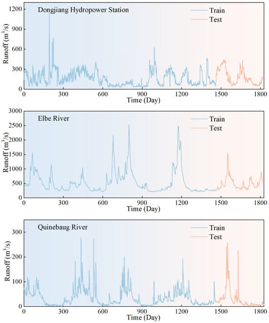
Figure 1. Initial daily streamflow series.

Table 2. Details of the three station and river datasets.

Station/River	Train		Test
	Time	Size	Time	Size
Dongjiang	1 January 1997–31 December 2000	1461	1 January 2001–31 December 2001	365
Elbe	1 January 1997–31 December 2000	1461	1 January 2001–31 December 2001	365
Quinebaug	1 January 1997–31 December 2000	1461	1 January 2001–31 December 2001	365

Although the dataset spans the period 1997–2001, this time window is suitable for the methodological objectives of this study. The selected dataset provides continuous, high-quality, and gap-free daily runoff records for all three stations, ensuring a stable observational baseline that allows the performance of the proposed SAEF framework and individual models to be evaluated under consistent hydrological conditions. Since the goal of this work is to verify the effectiveness and generalizability of the ensemble forecasting method rather than to conduct near-term climate-impact analysis, the use of historical data does not affect the scientific validity of the modeling framework.

3. Methodology and Experimental Setup

3.1. Machine Learning and Deep Learning

To build an SAEF model, we selected four representative base learners (SVM, LSSVM, LSTM, BiLSTM) according to the following criteria: (1) representativeness—covering kernel-based and least-squares kernel methods (suitable for trend and low-to-moderate nonlinearity) and gated recurrent neural networks (suitable for strong nonlinearity and temporal dependence); (2) complementarity—the models are expected to complement each other in handling smooth trends, peak responses, and seasonal transitions; and (3) reproducibility and computational feasibility—priority was given to models that train stably under our data size and experimental setup. Brief model-specific rationales are provided in the following subsections. In the data preprocessing stage, we converted continuous daily runoff data into input-output pairs required for supervised learning based on the idea of a sliding time window [43]. Specifically, we selected a sequence of length $M$ days as the input feature to forecast the runoff value of the first day in the future, thereby constructing a correspondence between the input sequence $[Z_1,Z_2,\dots ,Z_k]$ and the output target $[Z_{k+1}]$. This study determined the optimal input structure of machine learning and deep learning models through trial and error:

Step 1: Construct ML and DL models for different input lengths to forecast the future 1-day runoff of each watershed.

Step 2: Use Kling–Gupta Efficiency (KGE) as a model performance evaluation index to comprehensively measure the forecasting effects of different input lengths and model structures in each river basin. KGE comprehensively considers correlation, mean deviation, and variance ratio, and can reflect the forecasting ability of the model more comprehensively than a single error index.

Step 3: Based on the performance of the KGE index, select the optimal input length and model combination and apply it to subsequent integrated forecasting.

This study selected four ML and DL models that are relatively mature and representative in the field of hydrological forecasting, namely SVM, LSSVM, LSTM, and BiLSTM. These models have shown good performance in capturing the nonlinear characteristics and temporal dynamics of hydrological processes.

To ensure fair comparison and maintain controlled experimental conditions across different machine learning models, this study adopts a consistent hyperparameter strategy for SVM, LSSVM, LSTM, and BiLSTM. It is important to note that the primary objective of this research is not to optimize individual model configurations, but rather to develop and evaluate the proposed SAEF framework. For SVM and LSSVM, key hyperparameters such as the penalty parameter $C$, insensitive loss $\epsilon$, and the regularization and kernel parameters in LSSVM were manually adjusted through multiple preliminary trials to obtain stable and reasonably representative performance for runoff prediction. Similarly, the architectural hyperparameters of LSTM and BiLSTM—particularly the number of hidden units—were also fixed across all scenarios. By using consistent hyperparameters once reasonable configurations were selected, we ensure that the observed performance differences primarily reflect the intrinsic properties of the models rather than discrepancies arising from heterogeneous tuning strategies. This controlled experimental design strengthens the fairness, interpretability, and scientific rigor of the comparative analyses and the subsequent ensemble weight optimization. In addition, all hydrological inputs were normalized to the min–max scaling method to ensure stable model training and eliminate the influence of differing variable magnitudes.

3.1.1. Support Vector Machines

SVM was originally designed for binary classification tasks. By minimizing estimation error and achieving linear separation of inputs in a mapped high-dimensional feature space, SVM exhibits core advantages of low overfitting risk and excellent generalization ability, while supporting both linear and nonlinear classification as well as regression tasks.

Considering the rationality of training samples and data complexity comprehensively, and based on the principle of risk minimization, given a dataset $(x_i,y_i),x_i\in R_n,i=1,2,\dots ,m$ (where $x_i$ denotes input variables, $y_i$ corresponds to the respective output variables, and $m$ represents the number of variable dimensions), the decision function of the SVM model can be expressed as:

$$f(x)={\displaystyle \sum _{i=1}^m(a_i-a_i^{\ast })K(x_i,x)+b, 0\le a_i\le C , }0\le a_i^{\ast }\le C$$

(1)

In this formula, all samples $(x_i,y_i)$ corresponding to non-zero coefficients $(a_i-a_i^{\ast })\ne 0$ are support vectors; $a_i$ denotes Lagrange multipliers; $a_i^{\ast }$ is a parameter value solved via a constrained optimization problem involving the insensitive coefficient $p$; $b$ is a threshold determined based on training samples; $K(x_i,x)$ is a kernel function satisfying the Mercer condition (in the form of $K(x_i,x)=\varphi {(x)}^T\varphi (x_i)$); and $C$ represents a penalty factor that balances model complexity and fitting error.

Linear kernel, polynomial kernel, and radial basis function (RBF) are the three most widely used core kernel functions in SVM models. The linear kernel is suitable for linearly separable data, but monthly runoff time series exhibit significant complexity, making it inapplicable. The polynomial kernel suffers from numerous parameters and excessively high computational complexity; thus, it is generally not adopted. As a local kernel function, the RBF possesses extremely strong nonlinear mapping capability and demonstrates excellent performance in most sample scenarios, serving as the preferred choice when the appropriate kernel function is unknown. Consequently, this study employs the Gaussian radial basis kernel function, whose mathematical expression is given as follows:

$$K(x_i,x)=\exp (-g{‖x_i-x‖}^2)$$

(2)

In the formula, $g$ denotes the kernel function parameter with $g>0$.

The parameters of the SVM model were manually tuned through several preliminary experiments, and the final selected configuration was kept fixed in all experiments to maintain comparability with LSSVM under the same controlled settings.

3.1.2. Long Short-Term Memory

As an improved derivative of Recurrent Neural Networks (RNN), LSTM models share the same three-layer basic structure (input layer, hidden layer, output layer). Their core advantage lies in the integration of self-recurrent units, which can effectively memorize long-term sequential information and alleviate the problems of gradient vanishing and gradient explosion. The functionality of these self-recurrent units is jointly regulated by the forget gate ($f_t$), input gate ($i_t$), and output gate ($o_t$).

The core function of the forget gate ($f_t$) is to select the information to be discarded in the current unit during training. It receives the output $h_{t-1}$ of the previous unit and the input $x_t$ of the current unit, then nonlinearly maps them to an output vector $f_t$ with values in the range [0, 1] via the Sigmoid function, which acts on the unit state $C_{t-1}$ at the previous time step. Specifically, a value of 1 indicates “complete retention” of information, while 0 denotes “complete discard”. Its mathematical expression is given as follows:

$$f_t=\sigma (W_f\left[h_{t-1},x_t\right]+b_f)$$

(3)

where $h_{t-1}$ denotes the output vector of the previous neuron; $x_t$ is the input vector of the current neuron; $\sigma$ represents the sigmoid activation function; $W_f$ and $b_f$ are the weight matrix and bias vector of the network, respectively, which regulate the signal transmission intensity and baseline offset.

The input gate ($i_t$) is responsible for dynamically regulating the state update of the current unit. Firstly, it processes the input information via the Sigmoid function to select key features requiring update; subsequently, a candidate update vector ${\tilde{C}}_t$ with values in the range (−1, 1) is generated through the tanh activation layer; finally, the state of the current unit is updated by fusing the outputs of the two aforementioned parts. Its mathematical expression is given as follows:

$$i_t=\sigma (W_i\left[h_{t-1},x_t\right]+b_i)$$

(4)

$${\tilde{C}}_t=\tanh (W_c\left[h_{t-1},x_t\right]+b_c)$$

(5)

where $W_c$ denotes the weight matrix of the candidate cell state; $b_c$ is the bias vector of the candidate cell state; $W_i$ represents the weight matrix of the input gate; $b_i$ is the bias vector of the input layer; ${\tilde{C}}_t$ is the potential update vector of the cell state, which stores new feature information to be integrated.

After the data is processed by the forget gate and input gate, the unit state at the previous time step $C_{t-1}$ is updated to the current time step state $C_t$. During the update process, the previous state $C_{t-1}$ is first multiplied by the forget gate output $f_t$ to filter and retain information, followed by fusing the candidate update vector generated by the input gate $i_t$ at time $t$ to obtain the current unit state $C_t$. The specific equation is given as follows:

$$C_t=f_t{C}_{t-1}+i_t\tilde{C}$$

(6)

The output gate ($o_t$) generates the output $h_t$ based on the current unit state $C_t$. Its working mechanism is as follows: first, the Sigmoid function is used to select the feature information to be output from the current unit state; subsequently, the unit state is normalized by the tanh function is multiplied by the output of the Sigmoid function, and finally, the output $h_t$ at the current time step is obtained. The specific equation is given as follows:

$$o_t=\sigma (W_o\left[h_{t-1},x_t\right]+b_o)$$

(7)

$$h_t=o_t\tanh (C_t)$$

(8)

where $W_o$ denotes the weight matrix of the output gate; $b_o$ is the bias vector of the output gate; $h_t$ represents the output vector of the unit at the current time step, which transmits effective feature information to the next unit.

Although LSTM models typically benefit from larger datasets, the daily runoff series used in this study (1826 samples) provides a sufficient time span for training medium-sized recurrent architectures commonly applied in hydrological forecasting. In addition, all hydrological inputs were normalized using the min–max scaling method to stabilize gradient propagation during training. To ensure methodological fairness, the number of hidden units and the overall architectural configuration of the LSTM model were fixed across all basins and experiments. Furthermore, the 1826-day daily runoff record provides sufficient temporal continuity for both recurrent models to extract seasonal hydrological patterns, ensuring that their performance comparison is not undermined by data sparsity. This controlled design guarantees that the comparison with BiLSTM and kernel-based models reflects intrinsic model behavior rather than differences in hyperparameter tuning.

3.1.3. Least Squares Support Vector Machine

LSSVM is a significant improved variant of the conventional SVM. As an extended form of SVM, LSSVM not only has a sound theoretical framework but also optimizes the solution mechanism by converting the inequality constraints of SVM into equality constraints. Specifically, it replaces the complex quadratic programming problem in SVM with solving linear equations through constructing a loss function. Compared with the original SVM, LSSVM reduces computational complexity, significantly enhances training efficiency and prediction accuracy, and ensures reliable global optimality. Currently, this model has been widely applied in various fields, including time series forecasting. The core parameters of LSSVM are the bandwidth of the squared kernel function and the regularization parameter. The reasonable configuration of these two parameters is crucial to the generalization performance of the LSSVM model, and their values need to be determined in close combination with specific application scenarios and the characteristics of training samples. The detailed calculation process and mathematical expressions of the LSSVM model are as follows:

(1) Assume $n$ training sample data $(x_i, y_i)$ are given (where $i=1,2,\dots ,n,x_t\in R^d$,$y_i\in R$), with $x_i$ as the input variable and $y_i$ as the output variable. The modeling form of the LSSVM is expressed as:

In the formula, $\omega$ is the weight vector; $b$ is the bias term; $\phi (x)$ is the kernel space mapping function.

(2) Based on the principle of structural risk minimization, the evaluation problem of the LSSVM model can be transformed into an optimization problem:

$$\left\{\begin{array}{l}\min J={\displaystyle \frac{1}{2}}{\omega }^T\omega +{\displaystyle \frac{1}{2}}\gamma {\displaystyle \sum _{i=1}^n{\zeta }_i^2}\\ s.t.y_i={\omega }^T\cdot \phi (x)+b+{\zeta }_i\end{array}\right.$$

(9)

In the formula, $\gamma$ is the regularization parameter (with $\gamma >0$); ${\zeta }_i$ is the slack variable.

Construct the Lagrangian function, and solve the aforementioned optimization problem via the method of Lagrange multipliers:

$$L(\omega ,b,\zeta ,\alpha )=J(\omega ,\zeta )-{\displaystyle \sum _{i=1}^n{\alpha }_i\left[{\omega }^T\phi (x_i)+b+{\zeta }_i-y_i\right]}$$

(10)

In the formula, ${\alpha }_i$ denotes the Lagrangian function.

(3) When ${\displaystyle \frac{\partial L}{\partial \omega }}=0,{\displaystyle \frac{\partial L}{\partial b}}=0,{\displaystyle \frac{\partial L}{\partial \alpha }}=0,{\displaystyle \frac{\partial L}{\partial \zeta }}=0$, $\omega$ and $\zeta$ can be eliminated. By incorporating the kernel function $K(x_i,x_j)=\phi {(x_i)}^T\phi (x_j)$ that satisfies the Mercer condition, the solution process of the optimization problem can be simplified to a linear equation:

$$\left[\begin{array}{cccc}0& 1& \dots & 1\\ 1& K(x_1,x_1)+{\displaystyle \frac{1}{\gamma }}& \dots & K(x_1,x_n)\\ ⋮& ⋮& \hspace{1em}\hspace{1em}& ⋮\\ 1& K(x_n,x_1)& \dots & K(x_n,x_n)+{\displaystyle \frac{1}{\gamma }}\end{array}\right]\left[\begin{array}{l}b\\ {\alpha }_1\\ ⋮\\ {\alpha }_n\end{array}\right]=\left[\begin{array}{l}1\\ y_1\\ ⋮\\ y_n\end{array}\right]$$

(11)

The RBF is selected as the kernel function of the LSSVM model, and in this case:

$$\left\{\begin{array}{l}K(x_i,x_j)=\exp (-g{‖x_i-x_j‖}^2)\\ g={\displaystyle \frac{1}{2{\sigma }^2}}\end{array}\right.$$

(12)

where $\sigma$ denotes the kernel width; ${\sigma }^2$ represents the squared kernel width.

(4) Finally, the solved LSSVM model is expressed as:

$$f(x)={\displaystyle \sum _{i=1}^n{\alpha }_{i}K(x_i,x_j)+b}$$

(13)

Similar to SVM, the regularization parameter and kernel parameter of LSSVM were manually examined through multiple trials, and the resulting configuration was fixed throughout the study. This ensures that SVM and LSSVM operate under consistent and comparable hyperparameter conditions.

3.1.4. Bidirectional Long Short-Term Memory

The BiLSTM neural network is an advanced variant of the traditional Bidirectional Recurrent Neural Network (BRNN), which replaces conventional RNN units with LSTM units. Composed of two LSTM components (forward and backward), BiLSTM can effectively capture comprehensive feature representations by integrating historical and future information of the sequence. The hidden layer of the model consists of two parts: the forward LSTM unit state and the backward LSTM unit state. After historical sequences are transmitted from the input layer to the hidden layer, forward and backward computations are performed, respectively. By learning the past and future features of the sequence, BiLSTM ultimately generates the output results. The BiLSTM model was implemented under the same data volume, input normalization approach, and hyperparameter configuration as the LSTM model, ensuring that both models operate under fully comparable conditions. By keeping the architectural settings fixed throughout all experiments, any observed performance differences between LSTM and BiLSTM can be attributed solely to their directional processing mechanisms rather than variations in model configuration. This controlled setup enables a scientifically valid and meaningful comparison of the two recurrent architectures on the medium-sized hydrological time series used in this study.

3.2. Arctic Puffin Optimization

3.2.1. Standard APO Algorithm

APO is a newly proposed swarm intelligence optimization algorithm inspired by the efficient hunting strategies exhibited by Arctic terns during flight and underwater foraging. The algorithm simulates the behavioral characteristics of terns in different environments and is designed to include multiple stages, such as population initialization, aerial exploration, underwater development, and behavioral conversion, with the aim of achieving a balance between global search and local development and improving the ability to solve complex optimization problems.

(1)

Population initialization

In the initial stage of the APO algorithm, the distribution of the Arctic puffin population is abstracted as a set of candidate solutions. Each “puffin” represents a solution vector, whose position is initialized as follows:

$$q_i^0=L_b+\gamma \times (U_b-L_b)$$

(14)

In this context, $q_i^0$ denotes the position vector of the $i$th individual at the initial time, $L_b$ and $U_b$ denote the lower and upper bounds of each dimension in the search space, respectively, and $\gamma$ is a random vector uniformly distributed over the interval $[0,1]$.

(2)

Flight phase

The aerial flight phase simulates the behavior of puffins searching for prey in the air and diving quickly to catch it, and is mainly used for global exploration. First, the Levy flight mechanism is used to perform long-distance random jumps from the current position, with the following update formula:

$$v_i^{t+1}=q_i^t+(q_i^t -q_j^t )\times \mathrm{\Lambda }(d)+\delta$$

(15)

Among them, $v_i^{t+1}$ represents the updated position of the $i$th individual after the $t+1$th iteration, $q_j^t$ is the position of an individual randomly selected from the current population and different from $i$, $\mathrm{\Lambda }(d)$ is the Levy flight step length generated according to the problem dimension $d$, and $\delta$ is a random perturbation term that follows a standard normal distribution.

After completing its aerial search, the puffin quickly dives to catch its prey. This process is controlled by introducing a speed factor to scale the position. The updated formula is as follows:

$$u_i^{t+1}=v_i^{t+1}\times \theta$$

(16)

$$\theta =tan[(\zeta -0.5)\times \pi ]$$

(17)

where $\zeta$ is a random number in the $[0,1]$ interval. This mechanism helps to break out of local optima and enhance global search capabilities by dynamically adjusting the movement amplitude of individuals.

(3)

Underwater foraging stage

During the underwater foraging stage, puffins flexibly adjust their search strategies based on the distribution of food resources in the environment, with the aim of strengthening their local development capabilities. First, puffins use a cooperative encirclement strategy, with multiple individuals surrounding schools of fish to conduct group searches. The update formula is as follows:

$$s_i^{t+1}=\left\{\begin{array}{l}{q}_k^t+\varphi \times \mathrm{\Lambda }(d)\times (q_m^t -q_n^t ), ifϵ\ge 0.5\\ q_k^t+\varphi \times (q_m^t -q_n^t ), ifϵ<0.5\end{array}\right.$$

(18)

where $\varphi$ is the collaboration coefficient used to adjust the intensity of group cooperative search, $\epsilon$ is a random number in the $[0,1]$ interval, and $q_k^t$, $q_m^t$, and $q_n^t$ are different individual positions randomly selected from the current population.

If there is little food in the current search area, the puffin will enter enhanced search mode, expanding the search range through adaptive strides. The updated formula is:

$$y_i^{t=1} =s_i^{t+1}\times (1+\phi )$$

(19)

$$\phi =0.1\times (ϵ-1)\times {\displaystyle \frac{T-t}{T}}$$

(20)

where $T$ is the maximum iteration count, $t$ is the current iteration count, and $\phi$ is a factor that converges dynamically during the iteration process. It is used to control the step size and prevent premature convergence.

In addition, when predators are detected, puffins quickly avoid danger by flying away from the dangerous area. The updated formula is:

$$z_i^{t+1}=\left\{\begin{array}{l}{q}_i^t+\varphi \times \mathrm{\Lambda }(d)\times (q_p^t -q_q^t), ifϵ\ge 0.5\\ q_i^t+\eta \times (q_p^t -q_q^t), ifϵ<0.5\end{array}\right.$$

(21)

where $\eta$ is a random factor within the $[0,1]$ interval, used to adjust the intensity of avoidance behavior.

(4)

Behavior switching and population update

In order to achieve a balance between exploration and exploitation, APO integrates new solutions generated at each stage through a behavior switching mechanism, selects the optimal individuals based on fitness values, and updates the next generation population. Its update strategy is as follows:

$$p_i^{t+1}=s_i^{t+1}\cup y_i^{t+1}\cup z_i^{t+1}$$

(22)

Finally, select the $N$ individuals with the highest fitness as the new generation population:

$$q_i^{t+1}=To{p}_N(P_i^{t+1} )$$

(23)

3.2.2. Improved Arctic Puffin Optimization

In meta-heuristic optimization algorithms, achieving an efficient balance between global exploration and local exploitation is a key factor in ensuring the algorithm’s excellent performance. Although APO demonstrates certain advantages in both global and local search, standard APO still has limitations. To address the limitations of standard APO, this paper proposes an IAPO Algorithm. IAPO uses two strategies to enhance its ability to overcome these limitations:

(1)

Elite Opposition-Based Learning Method

The distribution characteristics of the initial population in the search space have a significant impact on the search efficiency and solution accuracy of intelligent optimization algorithms. However, from the execution process of the APO algorithm, the standard APO relies on a random method to generate the initial population, which to some extent suffers from uneven distribution and insufficient exploration, making the algorithm prone to getting stuck in local optima. To solve this limitation, the IAPO algorithm introduces an improved strategy of Elite Opposition-Based Learning to generate the initial population of Arctic puffins. This method uses elite information to guide the population to construct directional reverse samples and selects the optimal individuals through a competition mechanism, thereby improving the distribution quality of the initial population in the solution space [44].

Specifically, assume that the optimization variable is $d$ dimensional, and initially generate $N$ individuals, denoted as:

$$Z=\left\{Z_k=(z_{k,1},z_{k,2},\dots ,z_{k,d})\left|k=1,2,\dots ,N\right.\right\}$$

(24)

For each dimension $h$, define the minimum and maximum boundaries of that dimension in the current population as follows:

$${\theta }_h =\underset{k}{\min }(z_{k,h} ), {\varphi }_h =\underset{k}{max }(z_{k,h})$$

(25)

The corresponding elite reverse position can be calculated as:

$$z_{k,h}^{\ast } =({\theta }_{h }+{\varphi }_h)-z_{k,h}$$

(26)

where $z_{k,h}^{\ast }$ represents the reverse value of the $h$th individual in the $k$th dimension. To prevent reverse position out-of-bounds, when the calculation result exceeds the boundary range, a random perturbation repair mechanism is introduced:

$$z_{k,h}^{\ast } =rand({\theta }_{h },{\varphi }_h )$$

(27)

Subsequently, the original individual set is merged with its reverse sample to construct a candidate set containing $2N$ individuals. These individuals are then sorted according to their fitness values, and the top $N$ individuals with the best performance are selected as the final initial population.

(2)

Enhanced behavior conversion factor

The design of the behavior conversion factor largely determines the overall performance of the APO algorithm. In the original APO algorithm, the factor $B$ is defined as:

$$B=2\times \log ({\displaystyle \frac{1}{rand}})\times \left(1-{\displaystyle \frac{t}{T}}\right)$$

(28)

where $rand$ is a random number between 0 and 1.

In the APO algorithm, based on the behavior conversion factor $B$ and the threshold parameter $C$ (where the original APO algorithm sets $C=0.5$), the algorithm can dynamically switch search strategies during iteration: when $B>C$ the algorithm tends to perform global exploration; when $B\le C$, it switches to local development mode.

Although the original behavior conversion factor $B$ achieves a certain degree of balance between global exploration and local exploitation in the APO algorithm, its flexibility remains insufficient when dealing with complex optimization problems, manifesting as the global search phase potentially ending too early, leading the algorithm to become trapped in a local optimum. To overcome this limitation, this paper employs an improved behavioral transition factor $B^{\ast }$. This factor combines the nonlinear characteristics of the cosine function with the dynamic changes in the objective function’s fitness, enabling adaptive adjustment of the search strategy. This approach more effectively balances global exploration and local exploitation, thereby enhancing the algorithm’s performance in complex problems. The enhanced behavioral transition factor is defined as:

$$B^{\ast }=0.5+0.3\cos ({\displaystyle \frac{\pi t}{2T}})$$

(29)

The improved conversion factor $B^{\ast }$ is more suited to the search requirements of complex optimization problems by introducing a nonlinear decay mechanism. This factor utilizes the smoothing characteristics of the cosine function to achieve a smooth transition between global exploration and local development, reducing the violent fluctuations caused by strategy switching during the search process. At the same time, it retains the random perturbation component to enhance the algorithm’s ability to escape from local optima, thereby improving overall optimization performance.

3.3. Season-Aware Ensemble Forecasting

3.3.1. Ensemble Forecasting

To effectively integrate the prediction results of multiple data-driven ML and DL models, this paper adopts an integrated prediction method. This method mainly consists of two core steps: seasonal division and weight optimization combination.

(1)

Seasonal Division

Given that different models exhibit varying predictive performance across different scenarios, this paper first divides the original data into distinct predictive scenarios to more accurately capture the strengths of each model under specific conditions. Optimizing the weight distribution for each scenario helps to give full play to the complementary effects of each base model and improve the overall performance of the integrated forecast. Combining the seasonal characteristics of runoff data and model applicability, this paper further subdivides the annual runoff data into spring (March to May), summer (June to August), autumn (September to November), and winter (December to February of the following year) to achieve scenario segmentation on a seasonal scale.

(2)

Weight Combination Optimization

In this study, the daily runoff predictions from each individual model are first used as inputs for the subsequent ensemble integration. The IAPO aims to maximize the correlation coefficient R between the ensemble output and the observed runoff. During the optimization process, the search space of each weight variable is restricted to the interval $[0,1]$, ensuring non-negativity and feasibility. To further reduce the complexity of multi-variable optimization and maintain consistency among the ensemble components, an additional equality constraint is imposed such that the sum of all weights equals one. The resulting constrained weight optimization formulation is expressed as follows:

$${\displaystyle \sum _i^n{v}_i(s)}=1$$

(30)

where $v_i(s)$ is the weight of the daily runoff forecasting results of each ML and DL model in the forecasting scenario $s$.

3.3.2. SAEF Framework

In this study, we innovatively proposed an SAEF method that integrates DL, ML, integrated prediction strategies, seasonal division mechanisms, and improved intelligent optimization algorithms to improve the accuracy and stability of runoff prediction. Figure 2 shows the overall framework of the constructed model, and its specific implementation process is as follows:

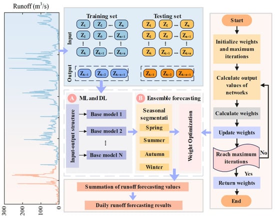
Figure 2. Framework of SAEF.

• In the machine learning and deep learning phase, the raw runoff data is first converted into an input-output structure, and various ML and DL models are used as base models for ensemble prediction to extract the feature representation capabilities of different models for the runoff process.
• In the ensemble prediction phase, the prediction results of each base model are divided into four independent scenarios—spring, summer, autumn, and winter—based on seasonal characteristics to enhance the model’s ability to perceive seasonal changes.
• Subsequently, through intelligent optimization algorithms, the weight combinations of the base models in each scenario are searched and optimized to construct a preliminary daily runoff forecasting model.
• Finally, the forecasting results of each base model are combined according to the weights determined by the optimization algorithm to obtain the final daily runoff forecast results, thereby accurately depicting future runoff trends.

3.4. Evaluation Indicators

To comprehensively evaluate the accuracy of the SAEF method in runoff prediction, this paper employs four commonly used performance evaluation metrics: Mean Absolute Error (MAE), Root Mean Square Error (RMSE), Nash–Sutcliffe Efficiency Coefficient (NSEC), and Kling–Gupta Efficiency (KGE). Among them, the closer the KGE and NSEC values are to 1, the better the model fit; the closer the MAE and RMSE are to 0, the smaller the forecasting error and the higher the model performance. The calculation formulas for the above indicators are as follows:

$$NSEC=1-{\displaystyle \frac{{\displaystyle \sum _{t=1}^n{(P_t-{\widehat{P}}_t)}^2}}{{\displaystyle \sum _{t=1}^n{(P_t-{\widehat{P}}_m)}^2}}}$$

(31)

$$RMSE=\sqrt{{\displaystyle \frac{1}{n}}{\displaystyle \sum _{t=1}^n{\left(P_t-{\widehat{P}}_m\right)}^2}}$$

(32)

$$MAE={\displaystyle \frac{1}{n}}{\displaystyle \sum _i^n\left|P_t-{\widehat{P}}_t\right|}$$

(33)

$$KGE=1-\sqrt{{(r-1)}^2+{(\alpha -1)}^2+{(\beta -1)}^2}$$

(34)

where $P_t$ is the actual value of the $t$th time, ${\widehat{P}}_t$ is the forecast value of the $t$th time, $P_m$ is the average value of the actual values, ${\widehat{P}}_m$ is the average value of the forecast values, and $r$ is the linear correlation coefficient between the observed values and the forecast values, reflecting the degree of correlation between the two. $\alpha$ is the ratio of the standard deviation of the forecast value to the standard deviation of the observed value, which is used to measure the consistency of the fluctuation range between the two; $\beta$ represents the ratio between the mean value of the forecast value and the mean value of the observed value, which is used to evaluate the deviation between the two in terms of magnitude.

3.5. Experimental Set

In this study, we introduced four representative ML and DL models, namely SVM, LSSVM, LSTM, and BiLSTM, to enhance the stability and accuracy of runoff prediction. Among them, the SVM and LSSVM models use RBF as kernel functions, and consistent hyperparameters are set during training to ensure model comparability. In the deep learning part, the LSTM and BiLSTM network structures both contain a hidden layer with 100 hidden units and a linear regression output layer to adapt to the regression characteristics of runoff forecasting. To avoid overfitting of the model, an early stopping mechanism was introduced during training. At the same time, all neural network models were trained using the Adam optimizer, and the initial learning rate was uniformly set to 0.0001. Additionally, to ensure fair comparison among models, the input delay length, training and testing set partitioning methods, and evaluation metric systems were kept consistent across all models. For the optimization algorithm, the number of iterations was set to 1000. For IAPO, APO, and SMA, the number of individuals created per iteration was fixed at 100. Detailed parameter settings are shown in Table 3.

Table 3. Hyperparameter settings for various models.

Model	Parameter	Value
LSTM, BiLSTM	Batch size	32
	Learning rate	0.0001
	Optimizers	Adam
	Output layer activation function	Linear
	Hidden layer activation	tanh
	Hidden layer neuron number	100
SVM, LSSVM	Kernel	RBF
IAPO, APO, SMA	Iteration number	1000
	Initial population size	100

4. Result

4.1. Setup of Temporal Input–Output Sequences

In daily runoff prediction modeling, the setting of the input time window length has a significant impact on prediction accuracy. To fully explore the ability of each model to perceive runoff dynamics, this paper uses an experimental comparison method to systematically evaluate the performance of four models—SVM, LSSVM, LSTM, and BiLSTM—under different time delay inputs. By gradually adjusting the time window length and using KGE as the performance measurement standard, the input structure with the best performance on the validation set was selected as the final model input. The experimental results show that the model performance shows significant differences under different time step settings [45]. For example, in the daily runoff forecasting task of the Elbe River, BiLSTM achieved the highest KGE value under a 14-step lag input, showing that it has a stronger ability to capture daily runoff trends. SVM also achieved optimal performance with an input length of 14, although its optimal time window was not the largest in some daily runoff forecasting tasks. The above phenomenon shows that the degree of dependence on historical information varies among models and that a reasonable setting of the time delay structure has a positive effect on improving model performance.

To ensure fairness among models, this study evaluates all candidate input window lengths under identical experimental settings for SVM, LSSVM, LSTM, and BiLSTM within each basin. The optimal input length for each model is then selected strictly based on the highest validation KGE and subsequently applied to the ensemble prediction stage. Table 4 summarizes the performance of all models under different input window lengths across the three study basins, demonstrating the controlled and comparable selection process.

Table 4. KGE values under varying input delays for each model.

Station	Model	Input Time Window Size
		3	4	5	6	7
Dongjiang	SVM	0.6115	0.7299	0.8271	0.7692	0.7462
	LSSVM	0.8027	0.8577	0.8923	0.8812	0.8627
	LSTM	0.8934	09110	0.9069	0.8254	0.7934
	BiLSTM	0.7834	0.8455	0.9122	0.8652	0.8023
River	Model	Input Time Window Size
		12	13	14	15	16
Elbe	SVM	0.5296	0.5435	0.5354	0.5276	0.5018
	LSSVM	0.6050	0.6524	0.7080	0.6035	0.5218
	LSTM	0.7529	0.7653	0.7668	0.7662	0.7599
	BiLSTM	0.7135	0.7535	0.8099	0.7835	0.7514
River	Model	Input Time Window Size
		5	6	7	8	9
Quinebaug	SVM	0.8026	0.8103	0.8200	0.7935	0.7831
	LSSVM	0.7930	0.8248	0.8481	0.8147	0.7825
	LSTM	0.8014	0.8310	0.8692	0.8226	0.7962
	BiLSTM	0.8076	0.8535	0.8895	0.8703	0.8648

4.2. Forecasting Results of Individual Models

Figure 3 presents the runoff prediction results of the SVM, LSSVM, LSTM, and BiLSTM models in the Dongjiang River Basin, the Elbe River Basin, and the Quinebaug River Basin, with the curves clearly reflecting the seasonal characteristics of runoff in each region. Specifically, in the Dongjiang Hydrological Station subplot, the prominent high-peak segments concentrated around Day 60–120 and Day 180–240 correspond to the summer flood season with concentrated monsoon rainfall, while the flat and low-value segments around Day 270–360 represent the stable winter runoff period. In the Elbe River subplot, the moderate peak segments around Day 90–150 and Day 210–270 are the runoff processes driven by spring snowmelt and autumn rainfall, respectively, and the obvious low-flow segment around Day 150–210 is consistent with the basin’s summer low-runoff characteristics. In the Quinebaug River subplot, the scattered small-peak segments (around Day 60–90, Day 150–180, Day 240–270) are the complex surface runoff caused by impermeable clay layers in summer and autumn, and the stable low-flow segment after Day 300 belongs to winter runoff. Overall, the forecasting curves of each model can well track the measured runoff trends, but there are obvious differences in their performance under different seasonal conditions. To further quantify the forecasting performance, Table 5 provides comprehensive evaluation indicators (including MAE, RMSE, NSEC, and KGE) for the four machine learning and deep learning models in the three basins, and these overall indicators serve as the basis for the season-specific analyses presented in Section 4.2. In spring, runoff processes are typically relatively stable, with minimal impact from extreme rainfall events. In this context, the LSTM and LSSVM models demonstrate strong trend-fitting capabilities. For example, in the Dongjiang River basin, the LSTM model achieved an MAE of 18.615 m³/s and a KGE of 0.907, while the LSSVM model also delivered stable predictive performance (KGE = 0.892). In contrast, the SVM model has a certain degree of lag at this stage and is not sensitive to subtle changes. BiLSTM performs better in capturing time dependence and achieves high KGE values in spring forecasting in multiple basins, such as 0.8099 in the Elbe River Basin in Germany. Summer is usually the period with the most dramatic changes in runoff. Affected by heavy rainfall, runoff exhibits high-frequency, non-steady peak fluctuations. In this complex hydrological context, the fitting capabilities of SVM and LSSVM models significantly decline, making it difficult to accurately respond to sudden increases in peak runoff. For example, in the Quinebaug River basin in the United States, the RMSE of SVM reached 116.21 m³/s, with a KGE of only 0.820, while LSSVM showed some improvement but still exhibited deviations in extreme peak segments. In contrast, BiLSTM demonstrated exceptional nonlinear modeling capabilities, achieving an MAE of 60.497 m³/s and a KGE of 0.890 during the summer in this watershed, outperforming other models in capturing extreme events. In autumn, as rainfall intensity and frequency weakened, runoff fluctuations tended to stabilize. At this stage, LSSVM performed particularly well in stable sections, such as in the Elbe basin, where it achieved an MAE of 7.178 m³/s. The LSTM and BiLSTM models maintained good stability, but their advantages over LSSVM were reduced. Although the SVM model improved to a certain extent in autumn, the forecasting results still showed significant fluctuations. Winter is the period with the smallest forecasting error for all models. BiLSTM and LSTM performed well in the low-value segment. For example, in the Dongjiang River basin, BiLSTM had an RMSE of only 28.36 m³/s and a KGE of 0.912. Although SVM and LSSVM did not perform as well as deep learning models overall, they showed improvement in trend tracking ability. In particular, in the Quinebaug River basin, LSSVM showed better forecasting stability than LSTM in the valley value range, demonstrating strong low-flow response ability.

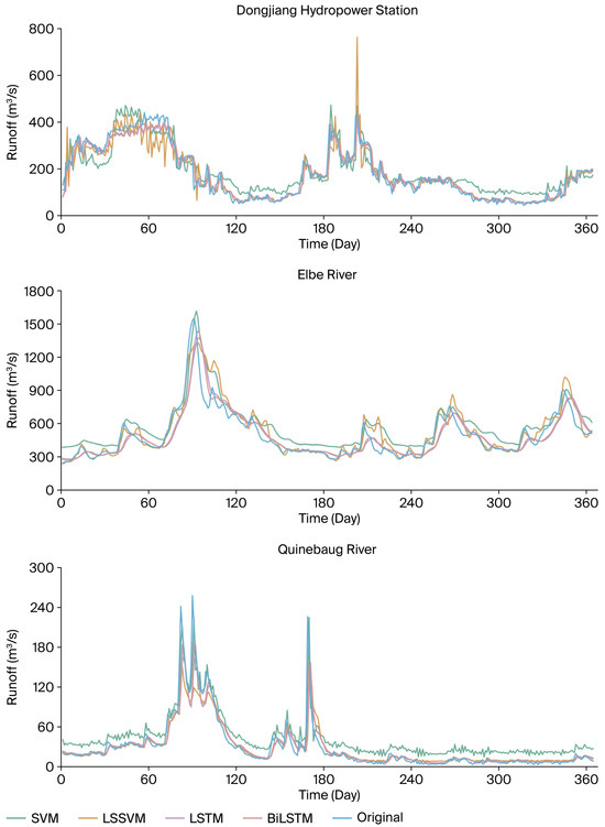
Figure 3. Comparison of single model daily runoff forecasting results.

Table 5. Results of individual model evaluation indicators.

Station/River	Model	Evaluation Indicators
		MAE (m3/s)	RMSE (m3/s)	NSEC	KGE
Dongjiang	SVM	40.436	48.550	0.816	0.827
	LSSVM	27.285	45.362	0.840	0.892
	LSTM	18.615	29.058	0.934	0.907
	BiLSTM	18.210	28.361	0.937	0.912
Elbe	SVM	15.859	18.501	0.709	0.535
	LSSVM	7.178	17.927	0.797	0.708
	LSTM	6.764	17.541	0.760	0.767
	BiLSTM	6.068	16.240	0.804	0.810
Quinebaug	SVM	96.974	116.210	0.789	0.820
	LSSVM	57.303	96.966	0.802	0.848
	LSTM	68.218	105.418	0.811	0.869
	BiLSTM	60.497	95.370	0.838	0.890

The experimental results indicate that the four models exhibit differences in their performance for runoff prediction across different seasons. BiLSTM performs optimally under the conditions of severe fluctuations in summer, effectively capturing complex temporal features; LSTM demonstrates stable trend-fitting capabilities across most seasons; LSSVM performs well during periods of relatively stable hydrological processes, such as in autumn and winter; and SVM has strong trend tracking capabilities in seasons with low fluctuations. Based on the advantages of each model in different scenarios, this paper selects SVM, LSSVM, LSTM, and BiLSTM as the base models for the SAEF method to take full advantage of their complementary characteristics and improve forecasting accuracy.

4.3. IAPO Performance

To evaluate the performance of the IAPO algorithm, this paper selected 10 representative functions from the CEC2019 test function set for experimental verification. The detailed information of the test functions is shown in Table 6. The CEC2019 function set is renowned for its complexity and challenge [46], covering various types of test functions, including single-peak functions and multi-peak functions. Single-peak functions contain only a single global optimal solution and are commonly used to assess an algorithm’s convergence efficiency and solution accuracy. Multi-peak functions, on the other hand, contain multiple local optimal points but only one global optimal solution. Such functions are primarily used to evaluate an algorithm’s search diversity and ability to escape local optima. Their complex structure significantly increases the difficulty of optimization, and many common algorithms struggle to obtain the global optimal solution when faced with such functions.

Table 6. Details of CEC2019 benchmark functions.

Functions	No	${\mathit{F}}_{\mathit{i}}^{\ast }={\mathit{F}}_{\mathit{i}}({\mathit{x}}^{\ast })$	Search Range	Dim
Storn’s Chebyshev Polynomial Fitting Problem	F1	1	[−8192, 8192]	9
Inverse Hilbert Matrix Problem	F2	1	[−16384, 16384]	16
Lennard-Jones Minimum Energy Cluster	F3	1	[−4, 4]	18
Rastrigin’s Function	F4	1	[−100, 100]	10
Griewangk’s Function	F5	1	[−100, 100]	10
Weierstrass Function	F6	1	[−100, 100]	10
Modified Schwefel’s Function	F7	1	[−100, 100]	10
Expanded Schaffer’s F6 Function	F8	1	[−100, 100]	10
Happy Cat Function	F9	1	[−100, 100]	10
Ackley Function	F10	1	[−100, 100]	10

To validate the effectiveness of the proposed improvement strategy and the overall performance of the improved algorithm, this study compared the experimental results of the IAPO algorithm with those of the original APO algorithm. Additionally, two intelligent optimization algorithms, SMA and Harris Hawk Optimization (HHO), which exhibit performance similar to APO, were introduced as reference algorithms. Considering that the CEC2019 benchmark function set imposes fixed requirements on problem dimensions, the dimension was uniformly set to 10 in the experiments. To ensure the fairness of the comparison results, the population size for all algorithms was set to 30, and the maximum number of iterations was set to 500. Each test function was run independently 30 times to reduce the bias caused by randomness. The control parameters for each algorithm were set according to the default configurations recommended in their original literature (see relevant literature). Table 7 presents the detailed performance evaluation results of all algorithms on the CEC2019 benchmark function set, with the optimal values for each metric highlighted in bold to emphasize their performance advantages. As shown in the results of Table 7, IAPO achieved significantly better optimization performance than other algorithms on most test functions, fully demonstrating its excellent optimization capability and stability. For the single-peak functions F2 and F3, IAPO outperforms APO, SMA, and HHO in both the average fitness value and standard deviation metrics, indicating its stronger convergence capability and local development efficiency when dealing with functions with simple structures and obvious gradient information. Although it failed to achieve the global optimal solution on F1, its results remained at a relatively optimal level, demonstrating the overall robustness of IAPO in single-peak function scenarios. In the multi-peak function tests from F4 to F10, IAPO achieved the lowest average values and standard deviations for most functions (such as F5, F6, F7, F8, and F9), indicating its excellent global search capability and result stability in complex search spaces. Especially for functions like F5 and F6 with multiple local extrema points, IAPO demonstrated a strong ability to escape local optima. Although it slightly lags behind some algorithms in the optimal results of F10, its average performance remains superior, reflecting its excellent generalization ability and algorithm robustness. By introducing an elite reverse learning initialization strategy into the APO algorithm, IAPO fully utilizes the spatial information of historical optimal solutions to construct a more representative and diverse initial population, effectively enhancing the algorithm’s global exploration capability in the early stages. Compared to traditional random initialization methods, this strategy significantly improves the coverage of the search space, reduces the unevenness of the initial solution distribution, and thus reduces the likelihood of getting stuck in local optima. Additionally, the reverse learning mechanism introduces a symmetric search mindset, enabling the algorithm to explore potential optimal solution regions based on known excellent solutions, thereby enhancing the depth of the search space exploration. The experimental results show that IAPO achieves better convergence accuracy and stability on multiple standard test functions, reflecting the algorithm’s balanced performance in terms of global optimization capabilities and local development efficiency. In practical applications, the improved strategy also shows good scalability, providing stronger model support and a theoretical basis for solving optimization problems such as highly complex hydrological forecasting.

Table 7. Performance comparison of IAPO against multiple algorithms on the CEC-2019 benchmark suite.

No	Index	IAPO	APO	SMA	HHO
F1	Avg	1.29	2.99	1.00	1.00
	Std	2.55	5.18	0.00	0.00
F2	Avg	4.31	5.89	4.99	4.99
	Std	3.86 × 10−2	1.52	3.98 × 10−2	4.25 × 10−2
F3	Avg	2.28	3.25	3.98	4.98
	Std	7.30 × 10−1	1.82	2.41	1.31
F4	Avg	4.59	9.86	2.04 × 10	5.11 × 10
	Std	3.13	4.21	8.03	1.56 × 10
F5	Avg	9.49 × 10−1	1.06	1.43	2.02
	Std	1.78 × 10−2	3.95 × 10−2	1.34 × 10−1	2.81 × 10−1
F6	Avg	9.89 × 10−1	1.00	4.72	8.28
	Std	5.12 × 10−4	7.60 × 10−4	1.72	1.60
F7	Avg	6.09 × 102	9.65 × 102	8.25 × 102	1.16 × 103
	Std	1.79 × 102	4.20 × 102	2.77 × 102	3.04 × 102
F8	Avg	2.36	3.88	4.08	4.75
	Std	1.77 × 10−1	3.81 × 10−1	4.14 × 10−1	2.64 × 10−1
F9	Avg	7.52 × 10−1	1.18	1.25	1.40
	Std	2.94 × 10−2	5.25 × 10−2	8.13 × 10−2	1.07 × 10−1
F10	Avg	1.12 × 10	1.64 × 10	2.06 × 10	2.12 × 10
	Std	1.81 × 10−1	8.53	3.64	1.11 × 10−1

4.4. SAEF Results

SVM, LSSVM, LSTM, and BiLSTM models exhibit significant predictive diversity across different seasonal scenarios. This diversity provides a foundation for constructing more robust ensemble prediction models. The initial prediction ensemble includes models with distinct structures and mechanisms, ensuring structural diversity among the base models. In the ensemble forecasting method proposed in this paper, the IAPO algorithm is introduced to optimize the weight combination of each base model. Table 8 shows the optimal weight configuration for different sites in the four seasons of spring, summer, autumn, and winter. From the weight distribution results, it can be seen that each base model has different advantages and disadvantages under different seasonal conditions, showing good complementarity, thereby improving the overall forecasting performance. For example, in the Dongjiang River Basin, BiLSTM achieved the highest weight of 0.6975 in winter, indicating its stronger temporal modeling and generalization capabilities during periods of relatively stable hydrological processes and smaller runoff fluctuations. In summer, LSTM obtained the highest weight of 0.6025, highlighting its excellent adaptability and dynamic capture capabilities when facing severe fluctuations in runoff caused by frequent sudden rainfall. In the Elbe River Basin in Germany, LSSVM achieved high weights of 0.6712, 0.4900, and 0.5534 in spring, summer, and autumn, respectively, indicating that its fitting stability is superior to other models in the context of low to medium runoff variability. BiLSTM dominated in winter with a weight of 0.6109, demonstrating excellent forecasting capabilities under conditions of low flow and small fluctuations. In contrast, in the Quinebaug River basin in the United States, SVM had higher weights in spring (0.5604) and summer (0.5414), indicating that it may still possess certain trend-tracking capabilities during high-flow periods with relatively stable trends; LSSVM dominated in winter (0.5974), further validating its effective fitting capability for valley intervals during stable periods.

Table 8. Weight distribution among four models.

Station/River	Model	Weight
		Spring	Summer	Autumn	Winter
Dongjiang	SVM	0.0266	0.0303	0.0503	0.0050
	LSSVM	0.4081	0.3419	0.4525	0.1473
	LSTM	0.1540	0.6025	0.2228	0.1502
	BiLSTM	0.4113	0.0253	0.2744	0.6975
Elbe	SVM	0.1416	0.1257	0.1993	0.1523
	LSSVM	0.6712	0.4900	0.5534	0.1129
	LSTM	0.0691	0.2305	0.1386	0.1239
	BiLSTM	0.1181	0.1538	0.1087	0.6109
Quinebaug	SVM	0.5604	0.5414	0.1056	0.2078
	LSSVM	0.0392	0.0823	0.2452	0.5974
	LSTM	0.3142	0.1822	0.2454	0.0832
	BiLSTM	0.0863	0.1941	0.4038	0.1116

To validate the effectiveness of the proposed SAEF method, Figure 4 and Table 9 present the performance comparison results between the SAEF method and four baseline models in daily runoff prediction tasks. Based on the comprehensive performance of multiple evaluation metrics, the SAEF model achieved the best prediction performance in the Dongjiang Hydrological Station, Elbe, and Quinebaug River Basin datasets, demonstrating its strong generalization ability across different basins and hydrological backgrounds. Specifically, at the Dongjiang Hydrological Station, the SAEF results had the lowest error level and optimal correlation performance, with MAE, RMSE, NSEC, and KGE of 14.965 m³/s, 20.130 m³/s, 0.968, and 0.935, respectively. In the Elbe River basin, the model also performed well, with the four metrics reaching 6.194 m³/s, 8.422 m³/s, 0.880, and 0.848, respectively. In the Quinebaug River basin, SAEF also achieved a significant advantage, with indicators of 51.629 m³/s, 74.137 m³/s, 0.906, and 0.931, respectively. The above results show that SAEF has good forecasting stability and accuracy in different hydrological situations. Further observation of the visualization results in Figure 5 shows that the SAEF model’s forecasting curves for the Quinebaug and Elbe river basins closely match the measured peak values, demonstrating its ability to accurately respond to extreme events during periods of high volatility. Although there were slight deviations in the forecasts for some peak periods at the Dongjiang station, SAEF was still significantly better than other single models in terms of overall trends and error distribution.

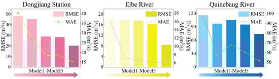
Figure 4. Comparison of results across model assessment metrics (SVM, LSSVM, LSTM, BiLSTM, SAEF). Note: Model1 to Model5 in the three subplots correspond to the five models, respectively: Model1 = SVM, Model2 = LSSVM, Model3 = LSTM, Model4 = BiLSTM, Model5 = SAEF.

Table 9. The MAE, RMSE, NSEC, and KGE values of the SAEF method and the four base models are used for daily runoff prediction.

Station/River	Model 1–5	Evaluation Indicators
		MAE (m3/s)	RMSE (m3/s)	NSEC	KGE
Dongjiang	SVM	40.436	48.550	0.816	0.827
	LSSVM	27.285	45.362	0.840	0.892
	LSTM	18.615	29.058	0.934	0.907
	BiLSTM	18.210	28.361	0.937	0.912
	SAEF	14.965	20.130	0.968	0.935
Elbe	SVM	15.859	18.501	0.709	0.535
	LSSVM	7.178	17.927	0.797	0.708
	LSTM	6.764	17.541	0.760	0.767
	BiLSTM	6.068	16.240	0.804	0.810
	SAEF	6.194	8.422	0.880	0.848
Quinebaug	SVM	96.974	116.210	0.789	0.820
	LSSVM	57.303	96.966	0.802	0.848
	LSTM	68.218	105.418	0.811	0.869
	BiLSTM	60.497	95.370	0.838	0.890
	SAEF	51.629	74.137	0.906	0.931

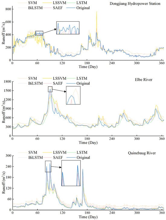
Figure 5. Comparison of SAEF results with four single machine learning/deep learning models.

Finally, to further analyze the stability of the predictive performance of each model, this paper introduces violin plots (Figure 6) to visualize the distribution of prediction errors on the test set. The results show that the SAEF model exhibits a more compact and symmetrical distribution across the three study basins, indicating smaller and more concentrated prediction errors with limited variability. The overall prediction results maintain high consistency and reliability across different samples. In contrast, the violin plots of the single model in some basins exhibit a more dispersed and skewed distribution pattern, reflecting its insufficient generalization ability when dealing with nonlinear dynamic and seasonal driving processes. This result further validates the SAEF method’s stable expression capability and error control efficiency in handling complex hydrological structures, demonstrating its stronger model coordination and cross-basin application value.

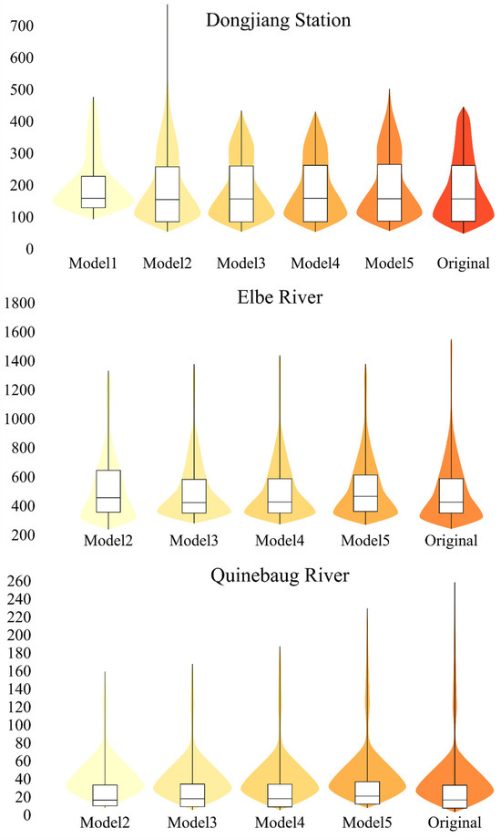
Figure 6. Distribution of violin patterns through model predictions.

5. Discussion

5.1. The Necessity of Seasonal Awareness

In the aforementioned experimental results (see Section 4.4), we observed significant differences in the predictive performance of different models across the four seasons. These differences are not only reflected in fluctuations in accuracy metrics but also highlight the non-stationary characteristics of hydrological processes across seasonal dimensions. Specifically, in the Dongjiang River basin, the ensemble weight of BiLSTM was significantly higher in winter than in other seasons (winter weight: 0.6975, summer weight: 0.0253), while LSTM had the highest weight in summer (0.6025), indicating its superior ability to model rapidly changing dynamic processes. Similar trends are also observed in the Elbe and Quinebaug river basins, further highlighting the decisive influence of seasonal variations on model selection and weight allocation. The above results reveal that runoff processes may be dominated by different hydrological drivers in different seasons, such as heavy rainfall events, snowmelt effects, or evaporation processes. Their intrinsic nonlinear response mechanisms and temporal scale differences make it difficult for a single model to simultaneously adapt to various hydrological states on an annual scale. Therefore, incorporating seasonal structures into the model optimization process is of great significance. Unlike traditional year-round unified modeling or studies that only divide the year into winter and rainy seasons [47], integrated methods with seasonal awareness are better able to respond to the hydrological characteristics of each season and dynamically adjust the model’s collaborative structure, thereby improving the generalization performance and forecasting stability of the overall system.

From a process perspective, the observed seasonal shifts in model dominance likely reflect the alignment—or misalignment—between the inductive biases of each algorithm and the dominant runoff generation mechanisms. During summer, when runoff is primarily driven by rapid surface responses such as convective rainfall and short flow pathways, models emphasizing sequential memory and nonlinear temporal filtering (e.g., LSTM) tend to perform more effectively. Conversely, in winter and low-flow periods, where storage–release dynamics and baseflow processes dominate, models capable of capturing bidirectional temporal dependencies (such as BiLSTM) or those based on stable nonlinear mappings in reconstructed lag spaces (such as LSSVM/SVM) show relatively better adaptability. These distinctions help explain why different models exhibit varying levels of success under different hydrological regimes.

Within this framework, the proposed SAEF approach utilizes the complementary characteristics of multiple learners and employs the IAPO algorithm to adaptively adjust ensemble weights according to seasonal hydrological conditions. The observed variations in optimized weights indicate that the model combination adapts differently to changing runoff generation patterns. Consequently, the seasonal awareness mechanism serves not merely as a means of enhancing forecasting accuracy but also as an initial attempt to connect data-driven modeling with the seasonal dynamics of hydrological processes. While the results demonstrate the framework’s promising stability and adaptability across different basins and seasonal contexts, further studies are needed to test its generalizability and interpretability under broader hydrological and climatic conditions.

5.2. Generalization Capability of the SAEF Method in Multi-Basin Environments

Empirical studies of three representative regions—the Dongjiang River Basin, the Elbe River in Germany, and the Quinebaug River in the United States—reveal significant differences in terms of basin area, topographic structure, and climatic conditions, which exert varying degrees of influence on the formation mechanisms of runoff processes. For instance, the Dongjiang River Basin is dominated by monsoon precipitation, resulting in relatively concentrated flood peaks; the Elbe River Basin exhibits pronounced seasonal precipitation and snowmelt influences; while the Quinebaug River basin is significantly influenced by temperate climate and human interventions (such as reservoir regulation), exhibiting more complex runoff fluctuation behavior. Table 10 lists the statistical information of representative hydrological characteristics in the three regions, further highlighting the differences in hydrological response mechanisms between basins. Such heterogeneity in hydrological sequences poses challenges to the generalization performance of models, especially during high-frequency flood peak responses or abnormal fluctuations in low-flow periods. However, the SAEF method proposed in this paper demonstrates strong adaptability. The model dynamically adjusts the combination weights of the base models by introducing an improved intelligent optimization algorithm (IAPO) and flexibly utilizes the structural advantages of each base model under different seasonal and basin conditions, effectively capturing complex hydrological patterns.

Table 10. Runoff profile in different hydrological regions.

Station/River	Mean (m3/s)	Min (m3/s)	Max (m3/s)	Median (m3/s)	Std (m3/s)
Dongjiang	167.02	29	1140	135.5	115.24
Elbe	520.45	200	2530	390	368.44
Quinebaug	36.24	0.57	278.36	21.5	36.96

It is particularly worth emphasizing that the SAEF method does not rely on the global adaptability of a single model, but instead constructs a combination system with local response capabilities through seasonal grouping and weight allocation strategies. This structure significantly enhances the model’s potential for promotion across multiple basins and climate zones. Overall, the model not only demonstrates strong structural adaptability in the data-driven training process but also maintains stable forecasting performance in the face of significant inconsistencies in hydrological behavior between basins.

To further reveal the seasonal adaptation patterns of the proposed SAEF framework, we extracted the gradient characteristics of prediction errors across humid regions (Dongjiang and Quinebaug) and the relatively drier temperate region (Elbe) based on the seasonal weight distributions shown in Table 7. The results indicate that climate-driven hydrological mechanisms substantially influence the seasonal distribution of forecasting errors, which is clearly reflected by the seasonal variations in model weights.

In the humid basins (Dongjiang and Quinebaug), rainfall exhibits strong seasonal concentration. During summer, intense convective storms lead to rapid runoff surges and sharp peaks. As a result, deep learning models with strong temporal-dependence capabilities, such as LSTM and BiLSTM, dominate the summer weights (e.g., Dongjiang: LSTM = 0.6025). Forecasting errors in these regions mainly originate from the uncertainty in capturing extreme peak responses. In winter, when the hydrological process is more stable and dominated by baseflow, BiLSTM achieves the highest weight (Dongjiang: 0.6975; Elbe: 0.6109), owing to its bidirectional temporal learning structure that effectively captures smooth seasonal transitions. Consequently, humid regions exhibit a clear “high-in-summer, low-in-winter” gradient in seasonal forecasting errors.

In contrast, the Elbe basin, influenced by a temperate continental climate, shows pronounced intra-annual hydrological variability. Summer experiences low rainfall and high evapotranspiration, while autumn and winter are affected by snow accumulation and melt processes. Under these conditions, LSSVM consistently achieves the highest weights in spring, summer, and autumn (0.6712, 0.4900, and 0.5534, respectively), reflecting its strong ability to capture deterministic trend components under low- to moderate-variability conditions. As summer runoff is relatively low and lacks sharp peak dynamics, deep learning models do not exhibit a clear advantage, resulting in a seasonal error pattern characterized by moderate gradients across seasons.

These findings highlight that:

(1)

Seasonal hydrological drivers (convective storms, snowmelt, or stable baseflow) determine the suitability of different models, forming identifiable seasonal error gradients.

(2)

Humid regions show a pronounced “summer-high, winter-low” error gradient due to concentrated storm-driven runoff.

(3)

In temperate climates with strong seasonal hydrological transitions, seasonal errors are more influenced by rainfall–snowmelt dynamics, with LSSVM dominating multiple seasons.

(4)

The seasonal variations in model weights align with basin-specific hydrological processes, demonstrating the physical interpretability of the SAEF framework.

5.3. Comparison with Existing Research

In recent years, some studies have attempted to incorporate seasonal information into hydrological prediction models to mitigate the impact of non-stationarity on model performance. For example, ref. [47] proposed a seasonal calibration framework based on the rainfall–runoff relationship, dividing the annual data into two segments: “rainy season” and “non-rainy season,” thereby enhancing the model’s adaptability to some extent. However, this dichotomy makes it difficult to fully characterize the subtle differences in hydrological drivers between different seasons. In contrast, this paper divides the annual data into four seasons (spring, summer, autumn, and winter) for daily runoff forecasting and constructs an integrated model substructure independently for each season. In the seasonal weight distribution, the model shows significant differences (e.g., the BiLSTM weight in the Dongjiang River Basin reaches 0.70 in winter, but only 0.03 in summer), indicating that independent modeling of the four seasons can more effectively capture the characteristics of seasonal non-stationary processes and achieve higher forecasting accuracy and stability in multi-basin experiments.

In terms of optimization algorithms, existing studies generally use swarm intelligence algorithms to optimize the parameters or weights of multiple models. However, the original APO algorithm is prone to premature convergence in high-dimensional continuous weight spaces, thereby limiting the fusion effect. This paper introduces two improvements based on this: first, an elite reverse initialization strategy is introduced to enhance the diversity of the initial solution; second, a cosine adaptive behavior conversion factor is adopted to dynamically balance global exploration and local exploitation capabilities during the search process. In the 10-dimensional optimization task of the CEC2019 benchmark function set, this improved strategy reduces the average error by 10.6% compared to the original APO and is first applied to the optimization of seasonal multi-model integration weights, significantly improving the rationality of fusion weight allocation and the generalization performance of the model.

In terms of applicability verification, most existing integrated forecasting methods only conduct experiments in a single climate zone and lack systematic verification across climate conditions, which limits the assessment of the stability and universality of the model in different basins. This paper conducted experiments in three basins with significantly different climate types and hydrological backgrounds: Dongjiang River in China (subtropical monsoon climate), Elbe River in Germany (temperate continental climate), and Quinebaug River in the United States (humid temperate climate). The results show that the proposed SAEF framework maintains high forecasting accuracy under different climate conditions, with an average RMSE across basins that is 48–58% lower than the best baseline model, significantly improving its adaptability under multi-regional conditions and filling the empirical gap in the cross-climate zone generalization verification of integrated forecasting models.

5.4. Discussion of Limitations

Although the proposed SAEF framework combined with the IAPO algorithm demonstrates significant advantages in daily runoff prediction—achieving high accuracy across three study basins and the CEC2019 benchmark tests—several limitations remain that merit further examination and improvement in future work.

First, computational and operational efficiency deserve attention. The SAEF framework simultaneously trains four types of base learners (SVM, LSSVM, LSTM, and BiLSTM) and repeatedly optimizes seasonal weights through the IAPO algorithm. This multi-stage process substantially increases training time and memory demand compared with single-model approaches, particularly when the dataset size or forecasting horizon expands. Such computational costs may constrain its deployment in real-time or resource-limited hydrological systems. Therefore, future studies should emphasize model lightweighting, parallel or distributed training, and hierarchical or approximate optimization strategies to maintain predictive accuracy while reducing computational overhead.

Second, the interpretability of the model and the weight-optimization mechanism remain limited. Although the IAPO-derived seasonal weights numerically reflect the relative contribution of each base learner, the underlying decision process and its correspondence to physical hydrological drivers are not yet transparent. This opacity may restrict trust and applicability in decision-support contexts. To address this issue, subsequent studies should incorporate interpretable machine-learning techniques—such as post-hoc sensitivity analysis, rule extraction, or physics-informed hybrid modeling—and perform correlation analyses between optimized weights and dominant hydrological variables. These efforts would enhance the physical explainability and credibility of model outputs for practical water-resources management.

Third, the framework is highly dependent on the quality and representativeness of historical observations. As a purely data-driven model, SAEF may exhibit reduced generalization when the training data contain gaps, measurement bias, or lack extreme events. Furthermore, while the seasonal segmentation improves responsiveness to periodic variations, its ability to capture non-periodic disturbances (e.g., extreme droughts, reservoir regulation, or human interventions) remains constrained. To overcome these issues, future research could integrate data assimilation, expand input features (such as meteorological forecasts, soil moisture, or remote-sensing indices), employ data-augmentation and semi-supervised learning techniques, and incorporate uncertainty-quantification frameworks (e.g., Bayesian or ensemble-based methods) to enhance robustness and provide credible confidence intervals under anomalous conditions.

In addition, the seasonal partition introduces a methodological trade-off. Dividing the annual data into four seasonal subsets improves local fitting and highlights seasonal hydrological mechanisms; however, it also reduces the sample size available for each submodel, which may increase overfitting risk and lead to discontinuities across seasonal boundaries. To balance these effects, future studies could explore overlapping windows, cross-seasonal transfer learning, regularization or penalty-term designs, and confidence-based sample reweighting strategies to retain the advantages of segmentation while mitigating statistical instability.

Finally, although the IAPO algorithm demonstrated superior performance to the original APO and other competing optimizers (showing a 10.6% reduction in average error on the CEC2019 10-dimensional benchmark tasks), all heuristic optimizers inherently remain sensitive to their hyperparameters and initial conditions. Their stability and reproducibility across different optimization landscapes or higher-dimensional weight spaces require further systematic sensitivity and robustness analyses. Enhancements such as multi-start initialization, hybrid optimization (e.g., combining global metaheuristics with local deterministic search or Bayesian optimization), and automated hyperparameter tuning should be considered to improve reliability in future applications.

In summary, while this study presents notable methodological and empirical progress, further research is needed to strengthen several aspects: computational efficiency for large-scale or real-time operation, physical interpretability, data completeness and robustness to anomalous events, the statistical balance introduced by seasonal segmentation, and the stability of the optimization process. Future work should prioritize lightweight model design, the integration of physical process knowledge to enhance explainability, and the incorporation of uncertainty quantification and online adaptive mechanisms into the SAEF framework. These improvements will facilitate its broader applicability and reliability in operational watershed management and real-time hydrological forecasting.

6. Conclusions

This study addresses the seasonal non-stationary characteristics of runoff processes and the generalization capability of models by proposing an SAEF method to enhance the accuracy and stability of daily-scale runoff prediction. Specifically, an initial set of prediction models, including SVM, LSSVM, LSTM, and BiLSTM, was first constructed to fully leverage the complementary advantages of machine learning and deep learning models in representing different hydrological characteristics. Subsequently, a seasonal partitioning mechanism is introduced to segment the annual data into four seasons (spring, summer, autumn, and winter) for modeling, thereby improving the model’s responsiveness to seasonal hydrological drivers. Additionally, this study designs an IAPO algorithm, which enhances the diversity of the initial population through an elite reverse initialization strategy and improves search efficiency and global optimal solution capability via dynamic behavioral transformation factors, thereby achieving adaptive optimization scheduling of multi-model integration weights. Experiments were conducted in three different basins and hydrological stations with distinct climatic and geographical backgrounds: the Dongjiang River, the Elbe River, and the Quinebaug River. The effectiveness of the improved optimization algorithm was validated using the CEC2019 benchmark function set. The applicability and advantages of the SAEF framework in complex hydrological scenarios were evaluated from multiple perspectives, leading to the following conclusions:

(1)

Unlike previous studies that applied a unified modeling framework throughout the year or divided the year into only two broad periods (rainy and non-rainy seasons), the SAEF method developed in this study incorporates a seasonal division strategy to better account for the seasonal non-stationarity inherent in hydrological processes. By independently modeling spring, summer, autumn, and winter periods, the proposed framework enables a more nuanced characterization of seasonal hydrological drivers and contributes to improved stability and flexibility in runoff prediction. Moreover, the ensemble structure facilitates complementary interactions among multiple models, offering a practical modeling approach for enhancing predictive performance under complex and varying hydrological conditions.

(2)

IAPO demonstrates significantly superior performance compared to the original APO and other advanced optimization algorithms (such as SMA and HHO) in the CEC2019 test functions. Among the 10 benchmark functions, IAPO achieved the optimal mean and standard deviation in most functions, particularly in single-peak and multi-peak functions such as F2, F3, F5, and F7, where it demonstrated smaller fitness values and more stable search performance, validating its performance advantages.

(3)

Unlike previous single-basin cases, the SAEF model achieved excellent daily runoff forecasting results under three different hydrological conditions. At the Dongjiang hydrological station, the SAEF model achieved MAE, RMSE, NSEC, and KGE values of 14.96, 20.13, 0.97, and 0.94, respectively; in the Elbe basin, the four metrics were 6.19, 8.42, 0.88, and 0.85; and in the Quinebaug basin, they were 51.63, 74.14, 0.91, and 0.93, respectively. The results also confirmed the robustness of the SAEF model for extreme peaks (with RMSE reduced by 48–58%) and low-flow periods (with KGE improved by 0.10–0.35), providing empirical evidence for the multi-regional application of the integrated method.

Although the method proposed in this paper demonstrates excellent accuracy and cross-basin adaptability in daily runoff prediction, there is still room for improvement. First, to enhance the model’s response speed and resource utilization efficiency in actual deployment, it is necessary to conduct in-depth research on model structure lightweighting, particularly in resource-constrained scenarios such as edge computing and real-time scheduling. Second, the current model mainly relies on data-driven mechanisms and lacks explicit modeling of hydrological physical processes. In the future, physical constraints or domain knowledge can be introduced to enhance the interpretability of the model and its generalization ability to non-observed scenarios. In addition, for more complex watershed management problems, the model needs to be extended to multi-step rolling forecasting and uncertainty quantification to improve its stability and reliability under multi-source input and multi-time lag conditions. In summary, follow-up work should focus on the comprehensive optimization of computational efficiency, interpretability, and practicality to promote the widespread application of intelligent runoff forecasting models in actual hydrological management.

References

- Xu, D.-M.; Liao, A.-D.; Wang, W.; Tian, W.-C.; Zang, H.-F. Improved monthly runoff time series prediction using the CABES-LSTM mixture model based on CEEMDAN-VMD decomposition. J. Hydroinform. 2023, 26, 255–283. [Google Scholar] [CrossRef]
- Seibert, M.; Merz, B.; Apel, H. Seasonal forecasting of hydrological drought in the Limpopo Basin: A comparison of statistical methods. Hydrol. Earth Syst. Sci. 2017, 21, 1611–1629. [Google Scholar] [CrossRef]
- Leach, J.M.; Kornelsen, K.C.; Coulibaly, P. Assimilation of near-real time data products into models of an urban basin. J. Hydrol. 2018, 563, 51–64. [Google Scholar] [CrossRef]
- Chen, L.; Wu, T.; Wang, Z.; Lin, X.; Cai, Y. A novel hybrid BPNN model based on adaptive evolutionary Artificial Bee Colony Algorithm for water quality index prediction. Ecol. Indic. 2023, 146, 109882. [Google Scholar] [CrossRef]
- Wang, W.-C.; Tian, W.-C.; Hu, X.-X.; Hong, Y.-H.; Chai, F.-X.; Xu, D.-M. DTTR: Encoding and decoding monthly runoff prediction model based on deep temporal attention convolution and multimodal fusion. J. Hydrol. 2024, 643, 131996. [Google Scholar] [CrossRef]
- Xu, X.; Wang, Z.; Zhou, F.; Huang, Y.; Zhong, T.; Trajcevski, G. Dynamic transformer ODEs for large-scale reservoir inflow forecasting. Knowl.-Based Syst. 2023, 276, 110737. [Google Scholar] [CrossRef]
- Xu, D.-M.; Zeng, Q.-Q.; Wang, W.-C.; Zhang, X.-T.; Wang, Y.-Y.; Zang, H.-F. A deep learning runoff prediction model based on wavelet decomposition and dynamic feature fusion. Sci. Rep. 2025, 15, 37235. [Google Scholar] [CrossRef]
- Roushangar, K.; Alizadeh, F. A multiscale spatio-temporal framework to regionalize annual precipitation using k-means and self-organizing map technique. J. Mt. Sci. 2018, 15, 1481–1497. [Google Scholar] [CrossRef]
- Wang, W.-C.; Gu, M.; Hong, Y.-H.; Hu, X.-X.; Zang, H.-F.; Chen, X.-N.; Jin, Y.-G. SMGformer: Integrating STL and multi-head self-attention in deep learning model for multi-step runoff forecasting. Sci. Rep. 2024, 14, 23550. [Google Scholar] [CrossRef]
- Beven, K.J.; Kirkby, M.J.; Freer, J.E.; Lamb, R. A history of TOPMODEL. Hydrol. Earth Syst. Sci. 2021, 25, 527–549. [Google Scholar] [CrossRef]
- Dai, X.; Wang, L.; Cao, Q.; Niu, Z.; Luo, Z.; Luo, Y. Assessing the Hydrological and Social Effects of Three Gorges Reservoir Using a Modified SWAT Model. J. Earth Sci. 2025, 36, 1793–1807. [Google Scholar] [CrossRef]
- Blaskey, D.; Gooseff, M.N.; Cheng, Y.; Newman, A.J.; Koch, J.C.; Musselman, K.N. A High-Resolution, Daily Hindcast (1990–2021) of Alaskan River Discharge and Temperature From Coupled and Optimized Physical Models. Water Resour. Res. 2024, 60, e2023WR036217. [Google Scholar] [CrossRef]
- Valipour, M.; Banihabib, M.E.; Behbahani, S.M.R. Comparison of the ARMA, ARIMA, and the autoregressive artificial neural network models in forecasting the monthly inflow of Dez dam reservoir. J. Hydrol. 2013, 476, 433–441. [Google Scholar] [CrossRef]
- Zhang, G.P. Time series forecasting using a hybrid ARIMA and neural network model. Neurocomputing 2003, 50, 159–175. [Google Scholar] [CrossRef]
- Kouadio, K.L.; Kouame, L.N.; Drissa, C.; Mi, B.; Kouamelan, K.S.; Gnoleba, S.P.D.; Zhang, H.; Xia, J. Groundwater Flow Rate Prediction From Geo-Electrical Features Using Support Vector Machines. Water Resour. Res. 2022, 58, e2021WR031623. [Google Scholar] [CrossRef]
- Shi, W.; Wan, X.; Zhao, F.; Deng, R. A dual-model framework combining nonlinear autoregressive with exogenous inputs (NARX) and LSTM networks for enhanced daily runoff prediction and error correction. Environ. Model. Softw. 2025, 192, 106570. [Google Scholar] [CrossRef]
- Farfán-Durán, J.F.; Cea, L. Streamflow forecasting with deep learning models: A side-by-side comparison in Northwest Spain. Earth Sci. Inform. 2024, 17, 5289–5315. [Google Scholar] [CrossRef]
- Xu, D.-M.; Li, Z.; Wang, W.-C. An ensemble model for monthly runoff prediction using least squares support vector machine based on variational modal decomposition with dung beetle optimization algorithm and error correction strategy. J. Hydrol. 2024, 629, 130558. [Google Scholar] [CrossRef]
- Yan, X.; Chowdhury, N.A. Mid-term electricity market clearing price forecasting: A hybrid LSSVM and ARMAX approach. Int. J. Electr. Power Energy Syst. 2013, 53, 20–26. [Google Scholar] [CrossRef]
- Thanh, H.V.; Binh, D.V.; Kantoush, S.A.; Nourani, V.; Saber, M.; Lee, K.-K.; Sumi, T. Reconstructing Daily Discharge in a Megadelta Using Machine Learning Techniques. Water Resour. Res. 2022, 58, e2021WR031048. [Google Scholar] [CrossRef]
- Wang, W.-C.; Zhang, X.-T.; Tian, W.-C.; Li, Z.; Zhang, R.-G. Development and evaluation of a novel DTIB-LSSVM model for efficient and accurate runoff forecasting. Results Eng. 2025, 28, 108466. [Google Scholar] [CrossRef]
- Zhu, S.; Xu, M.; Wu, J.; Wang, Y.; Jiang, X.; Huang, Z.; Wang, Y.; Zhu, Y. A study on crude oil price forecasting model integrating CEEMDAN-VMD multiscale decomposition with CNN-BiLSTM. Results Eng. 2025, 27, 106391. [Google Scholar] [CrossRef]
- Wang, T.; Xu, Y.; Qin, Y.; Wang, X.; Zheng, F.; Li, W. Short-term PV forecasting of multiple scenarios based on multi-dimensional clustering and hybrid transformer-BiLSTM with ECPO. Energy 2025, 334, 137654. [Google Scholar] [CrossRef]
- Shahnazi, S.; Roushangar, K.; Hashemi, H. A novel implementation of pre-processing approaches and hybrid kernel-based model for short- and long-term groundwater drought forecasting. J. Hydrol. 2025, 652, 132667. [Google Scholar] [CrossRef]
- Chang, X.; Guo, J.; Liu, Y.; Wei, X.; Wang, X.; Qin, H. Study on runoff forecasting and error correction driven by atmosphere–ocean-land dataset. Expert Syst. Appl. 2025, 263, 125744. [Google Scholar] [CrossRef]
- Hu, W.; Zheng, M.; Cheng, J.; Wu, L.; Yao, J.; Cao, Y. Enhancing monthly runoff prediction in arid alpine basins of northwestern China by an EMD-PCA-LSTM hybrid model. J. Hydrol. Reg. Stud. 2025, 61, 102748. [Google Scholar] [CrossRef]
- An, H.; Ouyang, C. A hybrid framework for real-time flash flood forecasting in small ungauged catchments: Integrating hydrodynamic simulations with LSTM networks. J. Hydrol. 2025, 661, 133688. [Google Scholar] [CrossRef]
- Wei, Q.; Yang, J.; Fu, F.; Xue, L. Dynamic classification and attention mechanism-based bidirectional long short-term memory network for daily runoff prediction in Aksu River basin, Northwest China. J. Environ. Manag. 2025, 374, 124121. [Google Scholar] [CrossRef]
- Ng, K.W.; Huang, Y.F.; Koo, C.H.; Chong, K.L.; El-Shafie, A.; Najah Ahmed, A. A review of hybrid deep learning applications for streamflow forecasting. J. Hydrol. 2023, 625, 130141. [Google Scholar] [CrossRef]
- Ossandón, Á.; Rajagopalan, B.; Lall, U.; Nanditha, J.S.; Mishra, V. A Bayesian Hierarchical Network Model for Daily Streamflow Ensemble Forecasting. Water Resour. Res. 2021, 57, e2021WR029920. [Google Scholar] [CrossRef]
- Feng, Z.-K.; Niu, W.-J. Hybrid artificial neural network and cooperation search algorithm for nonlinear river flow time series forecasting in humid and semi-humid regions. Knowl.-Based Syst. 2021, 211, 106580. [Google Scholar] [CrossRef]
- Zounemat-Kermani, M.; Batelaan, O.; Fadaee, M.; Hinkelmann, R. Ensemble machine learning paradigms in hydrology: A review. J. Hydrol. 2021, 598, 126266. [Google Scholar] [CrossRef]
- Yang, W.; Ma, W.; Zeng, B.; Hao, Y. A crude oil price ensemble forecasting system based on outlier correction and adaptive error-compensation strategy. Eng. Appl. Artif. Intell. 2025, 160, 111856. [Google Scholar] [CrossRef]
- Gong, J.; Qu, Z.; Zhu, Z.; Xu, H.; Yang, Q. Ensemble models of TCN-LSTM-LightGBM based on ensemble learning methods for short-term electrical load forecasting. Energy 2025, 318, 134757. [Google Scholar] [CrossRef]
- Brodeur, Z.P.; Taylor, W.; Herman, J.D.; Steinschneider, S. Synthetic Ensemble Forecasts: Operations-Based Evaluation and Inter-Model Comparison for Reservoir Systems Across California. Water Resour. Res. 2025, 61, e2024WR039324. [Google Scholar] [CrossRef]
- Li, S.; Chen, H.; Wang, M.; Heidari, A.A.; Mirjalili, S. Slime mould algorithm: A new method for stochastic optimization. Future Gener. Comput. Syst. 2020, 111, 300–323. [Google Scholar] [CrossRef]
- Wang, Q.; Du, W.; Han, Y.; Xue, H.; Gao, B.; Dong, S.; Yang, M. Robust form finding of tree-like structure by improved slime mould algorithm. Eng. Struct. 2025, 336, 120421. [Google Scholar] [CrossRef]
- Wang, W.-C.; Tian, W.-C.; Xu, D.-M.; Zang, H.-F. Arctic puffin optimization: A bio-inspired metaheuristic algorithm for solving engineering design optimization. Adv. Eng. Softw. 2024, 195, 103694. [Google Scholar] [CrossRef]
- Snousy, M.G.; Elshafie, H.M.; Abouelmagd, A.R.; Hassan, N.E.; Abd-Elmaboud, M.E.; Mohammadi, A.A.; Elewa, A.M.T.; El-Sayed, E.; Saqr, A.M. Enhancing the prediction of groundwater quality index in semi-arid regions using a novel ANN-based hybrid arctic puffin-hippopotamus optimization model. J. Hydrol. Reg. Stud. 2025, 59, 102424. [Google Scholar] [CrossRef]
- Adnan, R.M.; Mostafa, R.R.; Kisi, O.; Yaseen, Z.M.; Shahid, S.; Zounemat-Kermani, M. Improving streamflow prediction using a new hybrid ELM model combined with hybrid particle swarm optimization and grey wolf optimization. Knowl.-Based Syst. 2021, 230, 107379. [Google Scholar] [CrossRef]
- Abaza, A.; El-Sehiemy, R.A.; Hamida, M.A.; Chenouard, R.; Bayomyi, A. Optimal parameter extraction of equivalent circuits for single- and three- phase Power transformers based on arctic puffin algorithm accomplished with experimental verification. Results Eng. 2025, 26, 104888. [Google Scholar] [CrossRef]
- Heinemann, N.; Yang, S.; Büttner, O.; Borchardt, D. Nutrient loading and stream order shape benthic and pelagic spring algal biomass in a large, temperate river basin (Elbe River). J. Environ. Manag. 2025, 383, 125440. [Google Scholar] [CrossRef] [PubMed]
- Wang, J.; Li, X.; Wu, R.; Mu, X.; Baiyinbaoligao; Wei, J.; Gao, J.; Yin, D.; Tao, X.; Xu, K. A runoff prediction approach based on machine learning, ensemble forecasting and error correction: A case study of source area of Yellow River. J. Hydrol. 2025, 658, 133190. [Google Scholar] [CrossRef]
- Yuan, Y.; Mu, X.; Shao, X.; Ren, J.; Zhao, Y.; Wang, Z. Optimization of an auto drum fashioned brake using the elite opposition-based learning and chaotic k-best gravitational search strategy based grey wolf optimizer algorithm. Appl. Soft Comput. 2022, 123, 108947. [Google Scholar] [CrossRef]
- Moosavi, V.; Gheisoori Fard, Z.; Vafakhah, M. Which one is more important in daily runoff forecasting using data driven models: Input data, model type, preprocessing or data length? J. Hydrol. 2022, 606, 127429. [Google Scholar] [CrossRef]
- Hasan, D.O.; Mohammed, H.M.; Abdul, Z.K. Griffon vultures optimization algorithm for solving optimization problems. Expert Syst. Appl. 2025, 276, 127206. [Google Scholar] [CrossRef]
- Metzger, A.; Marra, F.; Smith, J.A.; Morin, E. Flood frequency estimation and uncertainty in arid/semi-arid regions. J. Hydrol. 2020, 590, 125254. [Google Scholar] [CrossRef]
Disclaimer/Publisher’s Note: The statements, opinions and data contained in all publications are solely those of the individual author(s) and contributor(s) and not of MDPI and/or the editor(s). MDPI and/or the editor(s) disclaim responsibility for any injury to people or property resulting from any ideas, methods, instructions or products referred to in the content. |
© 2025 by the authors. Licensee MDPI, Basel, Switzerland. This article is an open access article distributed under the terms and conditions of the Creative Commons Attribution (CC BY) license (https://creativecommons.org/licenses/by/4.0/).