Robust Ensemble-Based Model and Web Application for Nitrogen Content Prediction in Hydrochar from Sewage Sludge

Abstract

Hydrochar is a carbon-rich material produced through the hydrothermal carbonization (HTC) of wet biomass such as sewage sludge. Its nitrogen content is a critical quality parameter, influencing its suitability for use as a soil amendment and its potential environmental impacts. This study develops a high-accuracy ensemble machine learning framework to predict the nitrogen content of hydrochar derived from sewage sludge based on feedstock compositions and HTC process conditions. Four ensemble algorithms—Gradient Boosting Regression Trees (GBRTs), AdaBoost, Light Gradient Boosting Machine (LightGBM), and eXtreme Gradient Boosting (XGBoost)—were trained using an 80/20 train–test split and evaluated through standard statistical metrics. GBRT and XGBoost provided the best performance, achieving R² values of 0.993 and 0.989 and RMSE values of 0.169 and 0.213 during training, while maintaining strong predictive capabilities on the test dataset. SHAP analyses identified nitrogen content, ash content, and heating temperature as the most influential predictors of hydrochar nitrogen levels. Predicting nitrogen behaviour during HTC is environmentally relevant, as the improper management of nitrogen-rich hydrochar residues can contribute to nitrogen leaching, eutrophication, and disruption of aquatic biogeochemical cycles. The proposed ensemble-based modelling approach therefore offers a reliable tool for optimizing HTC operations, supporting sustainable sludge valorisation, and reducing environmental risks associated with nitrogen emissions.

1. Introduction

Wastewater treatment plants (WWTPs) are major producers of sewage sludge (SS), which is generated in large quantities worldwide [1,2]. In the European Union, about 10.0 million tons of dry SS were produced between 2003 and 2006, and this value was projected to exceed 13.0 million tons by 2020 [3]. In China, data from the Ministry of Housing and Urban–Rural Development (MOHURD) indicate that, in 2018, 2321 municipal wastewater treatment plants treated 168.8 million m³ of sewage per day, resulting in 11.8 million tons of dry SS per year [4]. Although SS is rich in organic matter and nutrients and can thus be regarded as a potential resource, it also poses serious environmental risks. It may contain pathogens, heavy metals, polycyclic aromatic hydrocarbons (PAHs), and polychlorinated biphenyls (PCBs), so it is considered a hazardous material requiring appropriate management and disposal [5,6].

The hydrothermal carbonization (HTC) of SS has emerged as a promising route to manage waste while simultaneously recovering energy and nutrients [7,8]. Unlike conventional pyrolysis or gasification, HTC operates at moderate temperatures (typically 180–250 °C) under autogenous pressure in the presence of water, which makes it particularly suitable for processing high-moisture feedstocks such as SS, food waste, and agricultural residues [9,10]. Under HTC conditions, wet biomass is converted into a carbon-dense, coal-like solid (hydrochar) through hydrolysis, dehydration, decarboxylation, and condensation reactions that resemble an accelerated form of natural coalification [11,12,13]. A key advantage of HTC is that it eliminates the need for energy-intensive drying, as water serves as the reaction medium. While carbon is concentrated in the hydrochar, substantial fractions of nitrogen, phosphorus, and potassium dissolve into the aqueous phase [14,15,16,17]. This not only enhances the fuel quality of hydrochar but also produces nutrient-enriched process water, contributing to circular bioeconomy strategies by generating both energy and agricultural inputs [18,19].

Beyond its potential as a solid fuel, SS-derived hydrochar has shown considerable promise as a soil amendment due to its ability to improve nutrient retention and soil quality. Moreover, modifying hydrochar can further enhance its agronomic performance. For example, Mg²⁺-loaded hydrochars demonstrate increased NO₃⁻ adsorption, helping reduce nitrate leaching and nutrient loss through water flow [20]. Similarly, functionalization with acidic groups increases surface acidity, promoting greater NH₄⁺-N adsorption, lowering soil pH, and reducing ammonia volatilization [21,22,23]. These characteristics highlight the dual environmental and agricultural benefits of hydrochar, reinforcing the importance of optimizing its physicochemical properties through controlled HTC processing.

Despite these advantages, the nitrogen content retained in the hydrochar can vary widely, depending on both the characteristics of the feedstock and HTC operating conditions. Important variables include the initial elemental composition of SS (e.g., carbon, hydrogen, nitrogen, oxygen contents) and its proximate analysis (volatile matter, fixed carbon, and ash content), as well as key HTC operating parameters such as reaction temperature, residence time, and total water in the reactor. Each of these factors can influence nitrogen transformation and retention in the hydrochar. Higher HTC temperatures generally reduce nitrogen retention in the solid product, as more nitrogen is converted into ammonia or other soluble species that migrate into the liquid phase [24,25]. Longer residence times can also promote the decomposition of nitrogen-containing compounds (such as proteins), resulting in increased nitrogen loss to the liquid phase, although time often has a less pronounced effect than temperature [25,26]. The composition of the feedstock is also crucial: SS with different organic fractions (for example, different protein or amino acid contents) can produce hydrochars with different nitrogen contents [27]. In addition, the pH of the reaction environment has been shown to affect nitrogen incorporation. Acidic conditions favour Maillard-type reactions that tend to enrich nitrogen in the hydrochar, whereas alkaline conditions are associated with reduced nitrogen content in the solid phase [28]. Understanding how each of these variables influences nitrogen fate is essential for tailoring HTC conditions, either to maximise nitrogen retention in the char (for nutrient-rich soil amendments) or to minimise it (for cleaner-burning solid fuels).

Given the complex and nonlinear interactions governing nitrogen content in hydrochar, machine learning (ML) offers a powerful tool for predicting nitrogen behaviour under diverse HTC conditions. Rather than relying solely on empirical correlations or extensive experimental campaigns, ML models can learn patterns from datasets that combine feedstock properties with process parameters. Advanced ML approaches have already shown high accuracy in biomass conversion studies by capturing intricate relationships between input variables and output properties. For instance, artificial neural networks (ANNs) have been used to predict the higher heating value and solid yield of SS-derived hydrochar from HTC conditions and elemental composition, achieving predictive accuracy with R² > 0.93 [15]. In another study, a Random Forest model was applied to estimate total phosphorus in SS hydrochar using different sets of predictors, including proximate and elemental analyses, total phosphorus in the original sludge (TP-SS), and HTC operating conditions, obtaining R² > 0.92 when P in SS was included [29]. Gradient Boosting Regression (GBR) has also been employed to predict phosphorus content and its transformation during the hydrothermal liquefaction (HTL) of SS, yielding average training and testing R² values greater than 0.95 and 0.85, respectively [30]. Furthermore, deep neural networks (DNNs) have been used to estimate hydrochar properties from the HTC of high-moisture municipal waste, with an average R² of 0.91 and RMSE of 3.29 and testing errors below 10% for higher heating values, carbon contents, and H/C ratios [31]. Several ML algorithms have also been employed in related thermochemical conversion studies. For example, this algorithm has been successfully applied to predict the carbon content and higher heating value of hydrochar [32] and to estimate energy recovery from hydrochar derived from wet organic wastes [33]. It has similarly been used to predict bio-oil yield and hydrogen content [34], as well as the carbon content and yield of biochar produced from biomass pyrolysis [35]. Moreover, ML techniques have supported uncertainty and sensitivity analyses for the co-combustion and pyrolysis of biowastes [36]. These studies further demonstrate the strong predictive capabilities of ML for modelling complex thermochemical processes.

Although these previous works demonstrate the usefulness of ML for modelling hydrochar characteristics from HTC of SS, fewer studies have focused specifically on predicting nitrogen content in hydrochar. One study trained a feedforward neural network using 138 data points that incorporated elemental composition, ultimate analysis, and HTC reaction conditions to predict hydrochar nitrogen content [37]. The final model, consisting of a two-layer structure with five neurons in the hidden layer, achieved R² values between 87.55% and 99.10% and RMSE values between 0.243 and 1.431 wt.% (dry basis) over 100 runs. Another study employed a multiple linear regression (MLR) model to predict the nitrogen content of SS-derived hydrochar [38]. Despite these advances, there remains substantial room for improvement by adopting ensemble learning algorithms such as eXtreme Gradient Boosting (XGBoost), Light Gradient Boosting Machine (LightGBM), AdaBoost, and Gradient Boosted Regression Trees (GBRT). Unlike ANNs, which rely on a single model, ensemble methods aggregate multiple learners to reduce both bias and variance, thereby improving generalisation and stability. Compared with MLR, ensemble techniques are not constrained by linearity assumptions and are better suited to capturing the nonlinear dependencies present in HTC systems. Their strength lies in iterative learning: Models are trained sequentially, and each new learner focuses on correcting the errors of its predecessors. By assigning greater weight to difficult cases, boosting-based ensembles progressively refine their predictions, achieving a better balance between complexity and generalisation than many traditional single-model approaches.

In this work, we address this gap by developing ensemble machine learning models capable of accurately predicting the nitrogen content of hydrochar produced from the hydrothermal carbonization of sewage sludge. Unlike previous studies, the present work integrates state-of-the-art ensemble learning algorithms with experimentally measured HTC data and further provides a practical web-based decision-support tool, enabling accurate and generalizable nitrogen-content predictions. We develop and compare several ensemble ML models to predict nitrogen content in hydrochar produced from HTC of SS. Four state-of-the-art ensemble algorithms—XGBoost, LightGBM, AdaBoost, and GBRT—are used to capture the relationships between input features (feedstock composition variables and process parameters) and the resulting nitrogen content of hydrochar. The models are trained on experimental data from HTC runs and validated against measured values from independent tests to ensure accuracy and robustness. Their performance is evaluated using standard statistical metrics (such as R² and RMSE), and rigorous validation, including cross-validation and testing on unseen data, is applied to confirm that the models generalise well beyond the training conditions. By comparing the performance of different algorithms, we identify the most accurate and reliable approach for nitrogen content prediction. The validated model is further interpreted using SHAP (SHapley Additive exPlanations) values to quantify the contribution of each input variable to nitrogen retention, thereby enhancing model transparency and supporting its use as a practical decision-support tool for researchers and industry professionals. Ultimately, this study shows how integrating advanced ML techniques with HTC experiments enables the accurate prediction of hydrochar nitrogen content, facilitating the optimisation of process conditions for both energy applications and nutrient recovery.

This study is structured as follows: Section 1 starts with a systematic review of the current literature. It focus on key obstacles in SS (SS) management, breakthroughs in HTC technology, and the use of ML in modelling hydrochar properties. Section 2 of this research covers the methodology and theoretical concepts behind ensemble ML algorithms. Section 3 describes data feature engineering and preprocessing. Section 4 examines the performance of these models in predicting hydrochar nitrogen content and benchmarks the results against classical ML techniques. This section also incorporates SHAP methodology to examine interpretability and find key process variables impacting nitrogen retention. Section 5 addresses the potential for optimizing HTC conditions, acknowledges the limitations of the methodology, and suggests directions for future research. This systematic framework is ready to shape the field of bioresource engineering by inspiring the novel application of ensemble-learning techniques for sustainable sludge valorization.

2. Materials and Methods

2.1. Research Methodology

The methodology for this research is outlined in Figure 1. The first step is gathering comprehensive data from previous studies. As shown in Figure 1, the predictors used to build our advanced ensemble ML model consist of several variables: nitrogen content (N%), oxygen content (O%), fixed carbon content (Fc%), ash content (A%), heating time (Ht, min), and heating temperature (HT, °C). Additionally, one output variable—nitrogen content—is considered. Data division into training and testing sets is the next step. Many researchers have emphasized that an 8:2 split is ideal for achieving a robust balance between model training and validation [39,40,41,42]. Our models consist of four ensemble methods, which are XGboost, GBRT, Lightgbm, and Adaboost. To improve efficiency and optimize our model, GridSearchCV will be implemented for hyperparameter tuning. In the GridSearchCV process, every specified hyperparameter in the grid is evaluated through five-fold cross-validation to ensure that the optimal combination is selected based on the performance metrics. The final optimized models obtained from GridSearchCV are then used to build our regression models and are tested on a hold-out test set to evaluate their predictive performance. The performance of the models is measured based on well-known performance metrics such as RMSE, MAE, and R². Visual evaluations such as scatter plot and the Taylor diagram are also included. Since our models work as black boxes, it is very important to explain the model using explainable ML techniques such as SHAP (Shapley Additive Explanations). Finally, our model is compared with single learner ML models in order to validate its performance improvements and assess its generalization capabilities relative to existing algorithms.

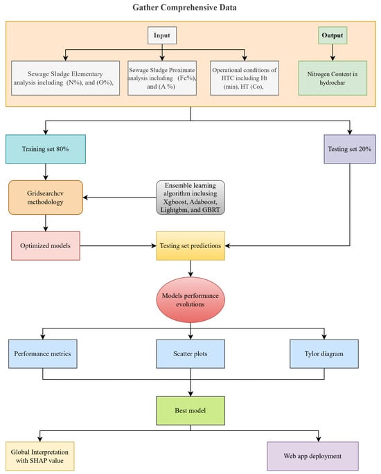
Figure 1. Study methodology.

2.2. Extreme Gradient Boosting (Xgboost)

XGBoost is an ensemble learning method introduced by Chen and Guestrin [43]. It boosts predictive performance by sequentially combining weak learners (e.g., decision trees), where each subsequent learner corrects errors from prior ones. A key innovation of the XGBoost algorithm is the incorporation of a regularization term into the objective function to mitigate overfitting.

The objective function O is defined as follows:

$$O=\sum _{i=1}^{n}L(y_i,F\left(x_i\right))+\sum _{k=1}^{t}R\left(f_k\right)+C$$

(1)

where $L(y_i,F\left(x_i\right))$ denotes the loss function measuring the prediction error for the i-th observation, $R\left(f_k\right)$ represents the regularization term for the k-th tree, C is a constant, and t is the total number of trees [44].

The regularization term $R\left(f_k\right)$ penalizes model complexity to avoid overfitting:

$$R\left(f_k\right)=\alpha H+{\displaystyle \frac{1}{2}}\eta \sum _{j=1}^H{w}_j^2$$

(2)

where $\alpha$ controls the complexity penalty per leaf, H is the number of leaves in the tree, $w_j$ denotes the weight (output value) of the j-th leaf node, and $\eta$ is the learning rate, which scales the contribution of each tree [44].

The XGBoost algorithm creates an ensemble of decision trees that are trained on a subsampled set. The algorithm identifies optimal feature splits for which their branching thresholds are constrained by maximum depth parameters [45]. It selects splits that maximize the predictive power of trees by continuous refinement. While training is ongoing, predictions from different trees are aggregated, and a weighted sum of those outputs yields the final prediction for the response variable [45].

2.3. Adaboost

Although AdaBoost is well known as a successful classifier, it can also be adopted for regression problems. This involves modifying its iterative error-correction mechanism to align with the goal of predicting continuous values. The AdaBoost regression problem emphasizes large residuals (discrepancies between predicted and true values). The process starts by training a weak regressor, such as a shallow decision tree, on the original dataset. Iteratively, weights for samples with significant differences between predicted and actual values are dynamically increased. This helps subsequent regressors focus on complex cases that were poorly predicted by earlier models. Given a dataset $D={\left\{(x_i,y_i)\right\}}_{i=1}^n$, where $x_i$ represents the input features and $y_i$ the corresponding target values, the algorithm works as follows:

Initially, all training samples are assigned equal weights:

$$w_i\left(1\right)={\displaystyle \frac{1}{n}},\forall i\in \{1,\dots ,n\}$$

(3)

In each iteration t, a weak regressor $h_t\left(x\right)$ is trained by minimizing the weighted squared error:

$${\mathrm{Error}}_t=\sum _{i=1}^n{w}_i\left(t\right){(y_i-h_t\left(x_i\right))}^2$$

(4)

The performance of the weak regressor is evaluated using an influence parameter ${\alpha }_t$, defined as

$${\alpha }_t={\displaystyle \frac{1}{2}}ln\left({\displaystyle \frac{1+{\rho }_t}{1-{\rho }_t}}\right)$$

(5)

The weights of incorrectly predicted samples are updated to give more importance to difficult cases:

$$w_i(t+1)=w_i\left(t\right)exp\left({\alpha }_t\left|y_i-h_t\left(x_i\right)\right|\right)$$

(6)

where ${\rho }_t$ is the weighted correlation between predictions and true values:

$${\rho }_t={\displaystyle \frac{{\sum }_{i=1}^n{w}_i\left(t\right)y_i{h}_t\left(x_i\right)}{{\sum }_{i=1}^n{w}_i\left(t\right)\left|y_i\right|}}$$

(7)

The weights are then normalized to maintain a valid probability distribution:

$$w_i(t+1)={\displaystyle \frac{w_i(t+1)}{{\sum }_{j=1}^n{w}_j(t+1)}}$$

(8)

The final AdaBoost regression model aggregates predictions from all weak regressors, weighted by their respective influence parameters:

$$F\left(x\right)=\sum _{t=1}^T{\alpha }_t{h}_t\left(x\right)$$

(9)

2.4. Gradient Boosting Regression Trees (GBRTs)

GBRT and AdaBoost differ mainly in their updating mechanisms. GBRT modifies regression targets by fitting new weak learners (trees) to residuals from the previous iteration. In contrast, AdaBoost modifies sample weights to prioritize misclassified instances, thereby improving classifier performance.

As shown in Figure 2, GBRT utilizes the gradient of these residuals, $r_m$, to fit new weak learners, iteratively improving prediction accuracy. GBRT employs Classification and Regression Trees (CARTs) as weak learners. The ensemble model is defined as

$$F_M\left(x\right)=\sum _{m=1}^{M}T(x;{\mathrm{\Theta }}_m)$$

(10)

where $T(x;{\mathrm{\Theta }}_m)$ represents a decision tree with parameters ${\mathrm{\Theta }}_m$.

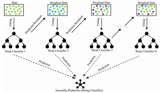
Figure 2. Illustration of the GBRT algorithm.

For regression tasks, GBRT relies on binary trees and loss functions such as mean squared error (MSE), absolute loss, and Huber’s loss. Huber’s loss combines the strengths of MSE and absolute loss, applying MSE to inliers (data near the model’s predictions) and absolute loss to outliers for robustness.

The residuals in GBRT are calculated as the negative gradient of the loss function:

$$r_m=-{\displaystyle \frac{\partial \mathrm{Loss}(y,F_{m-1}\left(x\right))}{\partial F_{m-1}\left(x\right)}}$$

(11)

This gradient-based update mechanism ensures systematic error correction, enhancing the model’s predictive performance.

2.5. Light Gradient-Boosting Machine (LightGBM)

LightGBM is a gradient boosting framework that uses a tree-based learning algorithm. In order to achieve high performance, it uses a technique knows as histogram-based splitting. Via this technique, continuous features are discretized into bins rather than evaluating every unique value during splits, which leads to a reduction in computational overhead [46]. Also, lightgbm has another innovation, which is exclusive feature bundling (EFB) [47]. EFB combines sparse or rarely co-occurring features into single bundles to minimize the effective number of features, lowering memory usage and complexity without sacrificing accuracy as a result. LightGBM also employs gradient-based one-sided sampling (GOSS) in order prioritize data points with large gradients (high errors) during training [48]. GOSS retains all high-gradient samples and randomly selects a subset of low-gradient ones, applying a weight multiplier to maintain unbiased learning. This focuses the model on challenging examples, improving accuracy with fewer data points. Additionally, LightGBM grows trees leaf-wise, expanding nodes with the highest error reduction first, unlike traditional level-wise growth, enabling faster convergence and efficient resource use. While designed for large datasets, LightGBM emphasizes computational efficiency rather than requiring minimal power. It reduces training time and memory demands compared to frameworks like XGBoost, making it suitable for resource-constrained environments or time-sensitive applications.

2.6. Data Splitting and Normalisation

Working towards building our models, the data is split into training and testing sets to ensure that the model’s performance can be properly tested on unseen data. To ensure no bias is introduced when building our models, the data is shuffled randomly before splitting. By carrying this out, we ensure that each subset is representative of the overall dataset. Usually, an 8:2 split is used, where 80% of the data is allocated for training, and the remaining is allocated for testing.

Additionally, normalization is applied to the dataset to standardize the range of input features. This process minimizes the impact of differing scales among the predictors, ensuring that each variable contributes equally to the model’s learning process. Techniques such as the min–max scaling or z-score standardization are commonly employed to achieve this normalization, thereby enhancing model convergence and overall performance. We use the min–max normalization technique, which scales the predictors into the range $[0,1]$. The following formula is used to represent this process:

$$x^{\prime }={\displaystyle \frac{x-\min \left(x\right)}{\max \left(x\right)-\min \left(x\right)}}$$

(12)

2.7. ML Model Development

To develop and optimize our model, various combinations of hyperparameters need to be tested to identify the best-performing combination. We often depend on methods like GridSearchCV that use cross-validation to compare different hyperparameter setups. The goal is to choose a setup that reduces prediction errors and, at the same time, enhances the model’s performance on unknown data. Whenever a new combination is tested, the training set is broken down into k folds. k–1 folds are used for training, while the left-out fold is used for testing. In this process, the prediction is repeated k times so that one fold becomes the test set each time. Figure 3 illustrates the Gridsearchcv process for hyperparameter tuning.

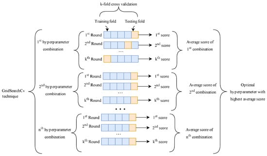
Figure 3. Gridsearchcv procedure.

Many hyperparameters are used to optimize the models’ performance. These hyperparameters directly influence the learning process, complexity, and generalization ability of the models. Among them, the learning rate represents the step size at which the model updates its predictions during training. A small learning rate, such as $0.001$ or $0.01$, lets the model learn more gradually, reducing the chance of overfitting. However, this demands a larger number of iterations to converge. On the other hand, a high value of the learning rate speeds up the training process but increases the chance of convergence to a suboptimal solution.

Additionally, the parameter $n\text{\_}estimators$ plays a critical role since it defines the number of boosting stages or weak learners combined to form the final prediction. Having more estimators can boost the model’s ability to capture complex patterns; however, overly large values may lead to overfitting and increased computational cost. In addition, $max\text{\_}depth$ represents the maximum depth of the decision trees used in the model. This feature helps control the complexity of the model by limiting the number of splits in the tree. A deeper tree can capture more complex patterns in the data, but it also increases the risk of overfitting, especially with limited training data. Conversely, a shallower tree may underfit the data, failing to capture important relationships.

The $num\text{\_}leaves$ parameter of the LightGBM model was also subjected to tuning. This hyperparameter controls the maximum number of leaves per tree and directly affects the model’s flexibility in dividing the data space. With a higher number of leaves, the model can capture finer details, whereas with fewer leaves, the model becomes simpler and more interpretable. Table 1 presents the optimized hyperparameter values for each model employed in this study.

Table 1. Best hyperparameter settings used for each ML model.

Models	Hyperparameters
	Max Depth	Learning Rate	Number of Estimators	Num Leaves
XGBoost	3.0	0.10	100	—
AdaBoost	—	1.00	100	—
LightGBM	—	0.20	500	31
GBRT	3.0	0.10	100	—

Lastly, to maintain the reproducibility and integrity of our experimental results, each machine-learning model was assigned a fixed $random\text{\_}state$ parameter within the Python 3.7 scikit-learn framework. This parameter regulates the randomization processes, such as the division of the dataset into training and testing subsets, ensuring identical sample allocations with each execution of the code. By setting $random\text{\_}state$ to a constant value, such as 42, we establish a stable foundation for performance comparisons across runs, which is essential for the robust validation of models. This practice also facilitates the precise replication of our study by others, reinforcing the credibility and scientific value of our findings.

2.8. SHapley Additive exPlanations

ML models in materials science often rely on ensemble techniques (such as random forests and gradient boosting) that excel at capturing complex composition–structure–property relationships but operate as black boxes. SHAP provides a principled way to interpret these models by attributing each prediction to individual features using game-theoretic Shapley values. This approach yields both local explanations (how each feature influences a single prediction) and global insights (which features are most influential overall). Lundberg and Lee’s original work on SHAP established that these feature attributions satisfy desirable properties like consistency, making SHAP a popular choice for explainable AI in materials research.

The Shapley values represent each feature’s contribution to the target and can be formally calculated as follows:

$${\varphi }_j=\sum _{S\subseteq \{1,\dots ,p\}\setminus \left\{j\right\}}{\displaystyle \frac{\left|S\right|!\left(p-\left|S\right|-1\right)!}{p!}}\left[f\left(S\cup \left\{j\right\}\right)-f\left(S\right)\right].$$

(13)

Here, p refers to the total number of features used by the model, and $f(·)$ is the prediction function of the ensemble model (for instance, a random forest or gradient boosting regressor). The term ${\varphi }_j$ captures the average marginal contribution of the j-th feature across all possible subsets of the other features.

In addition to examining individual Shapley values at the local level, researchers often seek a global measure of how important each feature is across the entire dataset. One common approach is to compute the average absolute Shapley value for feature j, denoted by $I_j$. Mathematically, this can be expressed as follows:

$$I_j={\displaystyle \frac{1}{n}}\sum _{i=1}^n\left|{\varphi }_j^{\left(i\right)}\right|,$$

(14)

where n is the total number of data points, and ${\varphi }_j^{\left(i\right)}$ is the Shapley value attributed to feature j in the i-th sample.

Lundberg produced an affective method named TreeShAP to deal with tree-based ensemble models. Different from the original SHAP, which relies on marginal expectations, TreeSHAP employs conditional expectations to more accurately estimate feature importance. Because the later method is computationally efficient, we employed it in our paper.

3. Database

A dataset of 159 data points was collected through earlier experimental investigations [37,49]. The dataset from previous research, which is also used in this study, was compiled from multiple independent experimental studies reported in the literature. These experiments were performed by different researchers, using different sewage sludge feedstocks, HTC reactors, temperatures, residence times, and analytical methods. Therefore, the dataset inherently includes real variability and heterogeneity across experimental conditions, providing a built-in external validation of the proposed ML models. The dataset contains different composition and properties of SS materials, including carbon (C%), hydrogen (H%), nitrogen (N%), oxygen (O%), volatile matter (V%), fixed carbon (Fc%), and ash content (A%), in addition to HTC operational conditions such as heating time (Ht) and heating temperature (HT). These composition and operational conditions were used as input variables, while nitrogen content in hydrochar (Nhc %) was utilized as the output. Although nine variables were initially evaluated, a collinearity filter was applied to ensure model robustness. Predictors exhibiting a pairwise correlation greater than 0.85 were removed to avoid redundancy. C, hydrogen H, and volatile matter V exceeded this threshold and were therefore excluded. The final model retained six variables—N, O, Fc, A, Ht, and HT—which showed acceptable correlation levels and contributed meaningfully to nitrogen content prediction. All subsequent analyses (correlation matrix, workflow, and SHAP plots) were generated using these six features. The dataset was divided into two subsets to facilitate model training and testing. The dataset was split into two subsets, with 80% allocated for model training and the remaining 20% reserved for testing. Table 2 provides the descriptive statistics analysis, such as the maximum and minimum values for each variable. Additionally, key statistical measures, including standard deviation (SD), standard error, skewness, and kurtosis, have been included to further characterize the dataset. As shown in Table 2, some variables, for example, O (%) has low standard deviations, which indicate that their values are closely clustered around the mean. On the other side, a higher standard deviation reflects greater variability in the data, as seen in the cases of Ht (min) and A (%), where the values are more widely dispersed. For instance, heating time (Ht (min)) exhibits a high standard deviation of 142.68, indicating significant variability in the data. Similarly, ash content (A (%)) shows a standard deviation of 14.05, reflecting a broad distribution of values. In order to evaluate the asymmetry of a probability distribution function, skewness is usually used as a statistical measure. According to Sharma and Ojha [50], skewness can take on a range of values, including zero, positive, negative, or remain undefined. A positive skewness indicates a distribution where the tail of the curve extends further to the right. In this dataset, variables such as Fc (%), A (%), and C (%) exhibit positive skewness, indicating a longer tail on the right side of the distribution. Conversely, O (%) and volatile matter V (%) display negative skewness, suggesting a longer tail on the left side. Also, Brown and Greene [51] stated that kurtosis is considered appropriate when its value falls between $-10$ and $+10$. Kurtosis helps determine whether a dataset has a light-tailed or heavy-tailed distribution compared to a normal distribution. This analysis provides useful insights into the shape of a probability distribution along the vertical axis [52].

Table 2. Descriptive statistics of the dataset.

Variable	Mean	Mode	Median	SE	SD	Variance	Kurtosis	Skewness	Max	Min
N (%)	4.80	5.29	4.75	0.139	1.753	3.073	0.938	0.466	8.85	1.21
O (%)	21.37	24.75	22.80	0.367	4.622	21.361	−0.277	−0.502	30.28	10.50
Fc (%)	6.00	3.90	5.14	0.295	3.723	13.861	0.676	0.883	18.55	0.70
A (%)	35.62	27.54	33.51	1.114	14.050	197.413	0.822	0.921	80.40	14.96
Ht (min)	99.06	30.00	45.00	11.315	142.676	20,356.383	6.335	2.626	720.00	0.00
HT (°C)	214.21	200.00	200.00	3.513	44.300	1962.511	1.518	0.642	380.00	100.00
Nhc (%)	3.07	2.10	2.40	0.170	2.137	4.569	1.478	1.355	9.29	0.39

The Pearson equation is a statistical measure used to assess both the strength and direction of the linear relationship between variables. This relationship is commonly denoted by the symbol ‘r’ [53]. The main purpose of this analysis is to identify correlations among parameters within a dataset. Evaluating multicollinearity and interdependency is essential for thoroughly understanding an ML model, as highlighted in previous studies [54]. These issues can introduce complexities that make interpreting the model more challenging. To analyze the the relationship between predictors themselves and with the output, a correlation matrix was constructed using Pearson’s correlation coefficient [55], considering seven input factors. The correlation values between different factors are presented in Table 3. This matrix is a symmetrical square matrix, where each $\left(xy\right)$th entry represents the correlation coefficient $R_{xy}$ between the xth and yth parameters. The diagonal elements, which represent the correlation of each parameter with itself, always have a value of one. The possible values range from $-1$ (indicating a perfect negative relationship) to 0 (no relationship) and to $+1$ (a perfect positive relationship). A positive correlation means that an increase in one parameter is associated with an increase in another, while a negative correlation means that an increase in one parameter is typically associated with a decrease in another. The sign of the correlation coefficient indicates the direction of the relationship. Pearson’s correlation coefficient is widely used in statistics and ML to evaluate and quantify the relationships between variables [56].

Table 3. Pearson’s correlation coefficients (r) between different variables in the dataset.

Variable	N (%)	O (%)	Fc (%)	A (%)	Ht (min)	HT (°C)	Nhc (%)
N (%)	1.000
O (%)	−0.095	1.000
Fc (%)	−0.029	0.436	1.000
A (%)	−0.529	−0.197	−0.078	1.000
Ht (min)	−0.032	0.187	−0.275	−0.023	1.000
HT (°C)	−0.044	−0.287	0.139	0.297	−0.113	1.000
Nhc (%)	0.865	−0.107	−0.055	−0.601	−0.178	−0.206	1.000

4. Results

4.1. Model Metric Performances Based on Training and Testing Set

During the training phase, both GBRT and XGBoost demonstrate outstanding performance based on values demonstrated in Table 4. Their $R^2$ scores are 0.993 and 0.989, respectively. Also, we can observe that their RMSE values are notably low at 0.169 for GBRT and 0.213 for XGBoost, while their MAE scores are also minimal (0.100 for GBRT and 0.140 for XGBoost). LightGBM also performs well in training with an $R^2$ of 0.987, RMSE of 0.231, and MAE of 0.155.

Table 4. Performance comparison of GBRT, AdaBoost, XGBoost, and LightGBM models based on $R^2$, RMSE, and MAE for training, testing, and all data.

Phase	Metrics	GBRT	AdaBoost	XGBoost	LightGBM
Train	$R^2$	0.993	0.933	0.989	0.987
	RMSE	0.169	0.532	0.213	0.231
	MAE	0.100	0.434	0.140	0.155
Test	$R^2$	0.973	0.935	0.979	0.960
	RMSE	0.389	0.602	0.342	0.470
	MAE	0.276	0.486	0.242	0.323
All data	$R^2$	0.988	0.934	0.987	0.981
	RMSE	0.231	0.547	0.245	0.295
	MAE	0.135	0.444	0.160	0.189

In the testing, XGBoost reaches the highest $R^2$ value with 0.979. The GBRT was next at 0.973. RMSE values in the testing phase are 0.342 for XGBoost and 0.389 for GBRT. They also achieved low MAE scores of 0.242 and 0.276, respectively. LightGBM maintains a strong performance with an $R^2$ of 0.960, RMSE of 0.470, and MAE of 0.323. AdaBoost, however, lags behind with a lower $R^2$ of 0.935, higher RMSE of 0.602, and MAE of 0.486.

When considering all the data points, we find that GBRT and XGBoost lead the performance metrics with overall $R^2$ scores of 0.988 and 0.987, respectively. The overall RMSE of GBRT is the lowest at 0.231, while XGBoost is the second lowest at 0.245. Their MAE scores are also lowest at 0.135 and 0.160, respectively. LightGBM’s metrics are an $R^2$ of 0.981, RMSE of 0.295, and MAE of 0.189. The AdaBoost algorithm still shows the lowest overall performance with an $R^2$ of 0.934, RMSE of 0.547, and MAE of 0.444.

4.2. Scatter Plot Evaluation for Ensemble Models

Figure 4 illustrates the relationship between the actual tensile strength (x-axis) and the predicted tensile strength (y-axis) for each of the developed models (GBRT, XGBoost, AdaBoost, and LightGBM) during both training and testing phases. In these plots, the slope of the trend line serves as a critical metric for evaluating the models’ ability to capture the relationship between experimental and predicted values [57]. A regression slope above 0.8 is often cited as indicative of a stronger correspondence between model predictions and actual observations [58]. Using the slope of the trend line offers several advantages over more traditional performance indicators such as R, MAE, or RMSE. First, it provides a direct measure of how well the model tracks the data across the full range of tensile strength values, rather than merely summarizing performance into a single statistic [59]. Second, by visually comparing the slope to the ideal 1:1 line, researchers can quickly assess whether the model systematically overestimates or underestimates the tensile strength. Consequently, the slope of the trend line complements existing metrics by offering a straightforward interpretation of predictive accuracy and model alignment with the observed data [60]. From the plots in Figure 4, it can be observed that both GBRT, XGBoost, and Lightgbm exhibit trend lines that closely match the ideal diagonal. This is a reflection of their near-perfect accuracy indicated by high R² values. On the other hand, AdaBoost shows somewhat lower slopes in comparison, but its performance stays within an acceptable range for reliable predictions. Generally speaking, these findings reinforce the superior forecasting performance of GBRT, XGBoost, and Lightgbm while confirming the viability of AdaBoost as a competitive alternative.

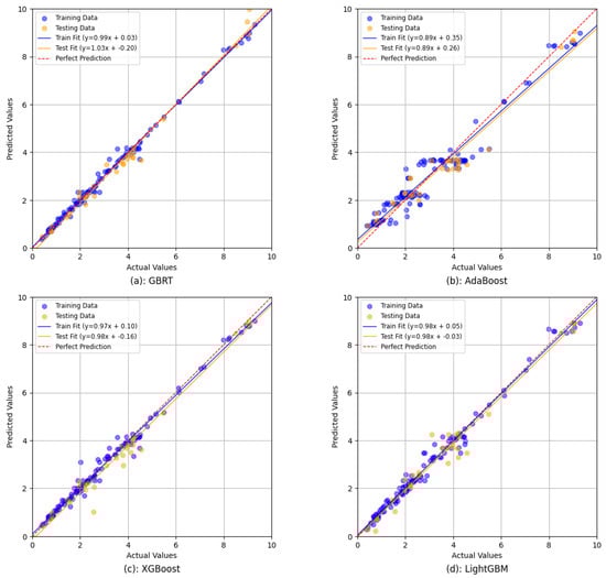
Figure 4. Scatter plots for ensemble ML models.

4.3. Error Assessment

Figure 5 shows the distribution of model residuals (i.e., the difference between the actual and predicted values) for each of the four developed models: XGBoost, GBRT, AdaBoost, and LightGBM. By looking at the shape and spread of these residual distributions, we can have valuable insights about how accurately each model captures the underlying data patterns. A tighter distribution centered around zero means that the model’s predictions are consistently close to the actual values, and this can reflect stronger predictive performance. From the plots in Figure 5, XGBoost and GBRT exhibit relatively peaked and symmetric distributions, which suggest that their residuals are more tightly clustered around zero. LightGBM, while still showing a concentrated distribution, displays a slightly broader spread, indicating a modest increase in the variance in its prediction errors compared to GBRT and XGBoost. In contrast, AdaBoost presents a noticeably wider and flatter distribution, with residuals more dispersed around zero. This suggests that AdaBoost’s predictions are subject to greater variability and, consequently, less consistent accuracy. In spite of these differences, all four models demonstrate reasonable alignment with the expected normal-like distribution of residuals, which can underline their robustness in capturing the overall trends of data. This confirms the earlier results where XGBoost and GBRT outperformed the other two models while still confirming the viability of LightGBM and AdaBoost for practical applications.

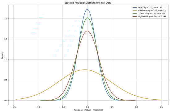
Figure 5. Normal distribution of ensemble models residuals.

Figure 6 presents the cumulative distribution function (CDF) of absolute residuals for all data points across the four developed models: GBRT, AdaBoost, XGBoost, and LightGBM. By analyzing the CDF curves, we can gain valuable insights into the predictive accuracy and error distribution of each model. A steeper curve that rises quickly and approaches a cumulative probability of 1 at lower residual values indicates that the majority of the model’s predictions are very close to the actual values, reflecting stronger predictive performance. From the figure, it is evident that the GBRT model exhibits the steepest and most left-shifted CDF, suggesting that its absolute residuals are generally the smallest among the four models. This indicates that GBRT consistently produces predictions that are very close to the true values. XGBoost and LightGBM also show relatively steep CDFs, closely following GBRT, which implies that these models also achieve high predictive accuracy with most residuals concentrated at lower values. In contrast, the AdaBoost model displays a much flatter and right-shifted CDF, indicating a wider spread of absolute residuals and a higher proportion of larger errors. This suggests that AdaBoost’s predictions are less consistent and more variable compared to the other models. Despite these differences, all models eventually reach a cumulative probability of 1, confirming that all residuals are accounted for. However, the clear separation between the CDFs highlights the superior performance of GBRT, XGBoost, and LightGBM over AdaBoost in terms of minimizing prediction errors.

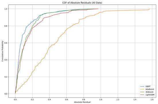
Figure 6. Cumulative distribution function for residual errors of ensemble models.

4.4. Comparing with Single Learner ML Algorithm

In this section, we compare the performance of the GBRT model with two widely used single learner models: K-Nearest Neighbors (KNN) and Support Vector Regression (SVR). The aim is to evaluate the effectiveness of ensemble learning against traditional single-model approaches in regression tasks. K-Nearest Neighbors is a non-parametric learning algorithm. The KNN algorithm works by looking at the k nearest points and their respective values to determine the value of a new point. The main hyperparameters that affect KNN are how many neighbors (k) to consider and the distance metric. The value of k controls how smooth the predictions are, while the distance metric determines how similarity is calculated. Picking a very small k can cause overfitting for predictions, while a large k can lead to underfitting problems. Support Vector Regression (SVR) is an extension of Support Vector Machines for regression problems. SVR attempts to fit the best possible line within a specified margin (epsilon) that covers as many data points as possible. The key hyperparameters for SVR include the kernel type (such as linear, RBF, or polynomial), which defines how the input data is transformed; the regularization parameter C, which balances model complexity and training error; and epsilon, which sets the margin of tolerance for error. To ensure a fair and optimal comparison, we used the Grid SearchCV methodology mentioned earlier to systematically explore and select the best hyperparameters for each model. This method helps in identifying the parameter combinations that yield the best validation performance. As shown in Table 5 and Figure 7, the GBRT model outperformed both KNN and SVR, with an R² of 0.9722, an RMSE of 0.3917%, and an MAE of 0.2842%. This means that GBRT’s predictions are, on average, closer to the true values and that it explains a greater proportion of the variance in the data. SVR and KNN perform less well, with higher RMSE and MAE values and lower R² scores, indicating less accurate and less reliable predictions. The KNN model achieved an R² of 0.9356, an RMSE of 0.5966%, and an MAE of 0.3643%. The SVR model achieved an R² of 0.9488, an RMSE of 0.5322%, and an MAE of 0.3899%. The superior performance of GBRT can be attributed to its ensemble approach, where a series of decision trees are built sequentially, with each tree correcting the errors of the previous ones. This allows GBRT to effectively capture complex, non-linear relationships in the data and reduce both bias and variance. In contrast, KNN and SVR, as single learner models, have limited capacity to model intricate patterns, especially in high-dimensional or noisy datasets. The flexibility and robustness of GBRT, combined with thorough hyperparameter tuning, explain why it achieves the best predictive performance in this comparison.

Table 5. Performance comparison of models on the test set.

Model	R2	RMSE	MAE
KNN	0.9356	0.5966	0.3643
SVR	0.9488	0.5322	0.3899
GBRT	0.9722	0.3917	0.2842

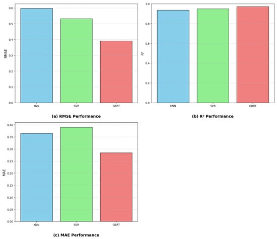
Figure 7. Model comparison: (a) RMSE; (b) R²; (c) MAE.

4.5. Taylor Diagram

A Taylor diagram represented by Figure 8 is an important plot used by statisticians to compare the performance of several models through a two-dimensional graph that simultaneously represents standard deviation (SD), root mean square error (RMSE), and correlation coefficient (R). In this plot each model is represented by a distinctively colored dot, while a star symbol on the x-axis denotes the reference statistics obtained from the experimental data (RMSE = 0, SD = 2.137, and R = 1). The performance of the model is measured by the closeness of its dot to this reference point. Black arcs that originate from the center and intersect with the axes indicate lines of a constant SD, whereas blue arcs radiating from the reference point represent lines of a constant RMSE. Black lines coming out from the center represents lines of constant R values. Overall, the positioning of a model with respect to the reference point offers a clear measure of its predictive accuracy, with the Adaboost model performing the least effectively and the GBRT model emerging as the most effective in predicting nitrogen content.

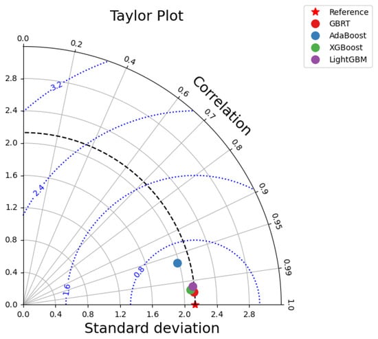
Figure 8. Taylor plot.

4.6. K-Fold Performance of Optimized GBRT

The generalization capability of the optimized GBRT model was further evaluated through a five-part cross-validation scheme. This approach reduces the influence of randomness in the training–testing process by splitting the dataset into five evenly sized groups. In every rotation, four groups are utilized to fit the model, while the remaining group is reserved for performance checking. This cycle is repeated a total of five times, and the overall performance is determined by averaging the outcomes from all iterations. Using this repeated validation strategy provides a stronger indication of the model’s robustness and allows for a clearer assessment of potential overfitting, particularly given the limited dataset size. The outcomes of this validation process for the optimized GBRT configuration are illustrated in Figure 9.

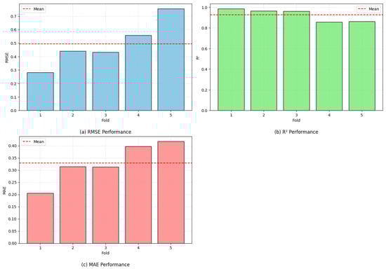
Figure 9. Performance of GBRT model across 5 folds.

The results show that although some variation occurs between the different validation rounds, the model consistently maintains strong predictive accuracy. The R² values span from 0.8572 to 0.9857, indicating reliable agreement with the observed data across all validation splits. Likewise, the RMSE ranges from 0.2815 to 0.7549, while the MAE varies between 0.2053 and 0.4175. These relatively small error values demonstrate that the model produces stable predictions throughout the repeated validation procedure. A detailed summary of all evaluation metrics is presented in Table 6.

Table 6. Performance measures for each fold.

Fold	RMSE	MAE	R2
Fold 1	0.2815	0.2053	0.9857
Fold 2	0.4413	0.3148	0.9651
Fold 3	0.4316	0.3130	0.9607
Fold 4	0.5574	0.3968	0.8572
Fold 5	0.7549	0.4175	0.8630
Mean	0.4933	0.3295	0.9263
Std. Dev.	0.1574	0.0751	0.0548
COV (%)	31.9	22.8	5.9

4.7. Shapley Method

Figure 10 presents the SHAP values for the predictors utilized in constructing the GBRT model to estimate nitrogen content. These SHAP values illustrate the local influence of each feature on the model’s output, with features ranked according to their relative importance. The feature exhibiting the broadest spread of SHAP values is recognized as the most significant contributor to the model’s predictions. Each SHAP value is calculated with respect to a baseline, which corresponds to the mean model prediction. Individual points on the plot represent the contribution of each feature for specific samples, with color encoding the feature value—blue indicating lower values and red denoting higher values.

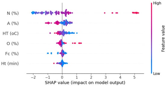
Figure 10. Shap importance variable plot.

Among the predictors, nitrogen (N %) demonstrates the widest distribution of SHAP values, particularly with pronounced positive contributions in red, signifying its dominant role in shaping the model’s output. This is followed by ash content (A %), heating temperature (HT °C), oxygen (O %), fixed carbon (Fc %), and heating time (Ht min), each contributing to varying extents. The results indicate that higher values of nitrogen and oxygen percentage in sludge are generally associated with increased nitrogen content, as evidenced by the clustering of red points on the positive side of the SHAP axis. Conversely, lower values of ash content and heating temperature, represented by blue points, tend to exert a positive impact on the model’s output. Overall, the SHAP summary plot underscores the pivotal influence of nitrogen, with ash content and heating temperature also playing substantial roles in the estimation process.

4.8. Web App

To enhance the practicality of our ML model, we developed an easy-to-use web app dashboard that allows users globally to predict the nitrogen content in the hydrochar produced after the hydrothermal carbonization process. We are using Streamlit to build interactive web apps easily and quickly. This tool facilitates fast deployment and provides an easy-to-use interface for researchers and practitioners to input critical process variables and obtain predictions of nitrogen content within seconds.

With an interactive dashboard, the need for specialized ML knowledge is reduced, allowing users to focus on results rather than code or computational processes. The dashboard based on Streamlit features a simple interface, enabling users to easily input variables like feedstock composition, HTC temperature, reaction time, etc. It then predicts the nitrogen content of hydrochar in numerical form through the interface. The application can be accessed at the following link: https://nitrogencontent-ffgcjngfjj7dbfbjh533k4.streamlit.app/ (accessed on 3 December 2025).

5. Limitations and Future Studies

This study shows that the use of ensemble machine learning (ML) can accurately predict the nitrogen content of hydrochar produced via hydrothermal carbonization (HTC). However, it does have limitations. One limitation of this model is that it can only make predictions based on data it has been exposed to, which is limited. The training data used here is derived from a few HTC experiments. Although these experiments encompass a wide variety of process parameters and feedstock properties, they may not sufficiently reflect the variability of real-world scenarios. The model’s performance could be improved through the incorporation of more experimental data or synthetic data generated via a validated process simulation. Future research may examine the extensibility of the ensemble ML model to a broader spectrum of feedstock types and reactor designs. Creating hybrid models that combine results from experiments and simulations could further enhance prediction accuracy under different hydrochar production conditions. Additionally, incorporating uncertainty quantification methods can provide clearer insights into a prediction’s confidence and reliability. Scaling up technology for large-scale commercial use is crucial for optimizing processes and operations.

6. Conclusions

In this research, we propose a new machine-learning-based model capable of accurately predicting the nitrogen content of hydrochar derived from the hydrothermal carbonization of sewage sludge. Four ensemble machine learning models were analyzed, and Gradient Boosting Regression Trees (GBRTs) and XGBoost were identified as the optimal models based on prediction accuracy. Our results show that ensemble models perform better than single learner algorithms for nitrogen content prediction.

Additionally, we utilized SHAP values to make our ensemble model’s predictions interpretable and to determine the most important predictor variables. The analysis revealed that the nitrogen content in hydrochar depends on the nitrogen and ash content of the sludge, as well as the heating time. A web application was developed that allows researchers, engineers, and practitioners to easily estimate nitrogen content in hydrochar using the proposed models. This tool provides practical applications and decision support for sustainable waste management and resource recovery of sewage sludge.

References

- Fu, Q.; Wang, D.; Li, X.; Yang, Q.; Xu, Q.; Ni, B.J.; Wang, Q.; Liu, X. Towards hydrogen production from waste activated sludge: Principles, challenges and perspectives. Renew. Sustain. Energy Rev. 2021, 135, 110283. [Google Scholar] [CrossRef]
- Huang, H.j.; Yang, T.; Lai, F.y.; Wu, G.q. Co-pyrolysis of sewage sludge and sawdust/rice straw for the production of biochar. J. Anal. Appl. Pyrolysis 2017, 125, 61–68. [Google Scholar] [CrossRef]
- Tarpani, R.R.Z.; Alfonsín, C.; Hospido, A.; Azapagic, A. Life cycle environmental impacts of sewage sludge treatment methods for resource recovery considering ecotoxicity of heavy metals and pharmaceutical and personal care products. J. Environ. Manag. 2020, 260, 109643. [Google Scholar] [CrossRef] [PubMed]
- Ministry of Housing and Urban-Rural Development. Statistical Yearbook of Urban and Rural Construction in China; Ministry of Housing and Urban-Rural Development: Beijing, China, 2020. [Google Scholar]
- Huang, H.j.; Yuan, X.z. The migration and transformation behaviors of heavy metals during the hydrothermal treatment of sewage sludge. Bioresour. Technol. 2016, 200, 991–998. [Google Scholar] [CrossRef]
- Xiao, X.f.; Chang, Y.c.; Lai, F.y.; Fang, H.s.; Zhou, C.f.; Pan, Z.q.; Wang, J.x.; Wang, Y.j.; Yin, X.; Huang, H.j. Effects of rice straw/wood sawdust addition on the transport/conversion behaviors of heavy metals during the liquefaction of sewage sludge. J. Environ. Manag. 2020, 270, 110824. [Google Scholar] [CrossRef]
- Wu, S.; Wang, Q.; Cui, D.; Wang, X.; Wu, D.; Bai, J.; Xu, F.; Wang, Z.; Zhang, J. Analysis of fuel properties of hydrochar derived from food waste and biomass: Evaluating varied mixing techniques pre/post-hydrothermal carbonization. J. Clean. Prod. 2023, 430, 139660. [Google Scholar] [CrossRef]
- Lee, J.I.; Jadamba, C.; Lee, C.G.; Hong, S.C.; Kim, J.H.; Yoo, S.C.; Park, S.J. Feasibility study of Aesculus turbinata fruit shell-derived biochar for ammonia removal in wastewater and its subsequent use as nitrogen fertilizer. Chemosphere 2024, 357, 142049. [Google Scholar] [CrossRef]
- Merzari, F.; Goldfarb, J.; Andreottola, G.; Mimmo, T.; Volpe, M.; Fiori, L. Hydrothermal carbonization as a strategy for sewage sludge management: Influence of process withdrawal point on hydrochar properties. Energies 2020, 13, 2890. [Google Scholar] [CrossRef]
- Pauline, A.L.; Joseph, K. Hydrothermal carbonization of organic wastes to carbonaceous solid fuel–A review of mechanisms and process parameters. Fuel 2020, 279, 118472. [Google Scholar] [CrossRef]
- Petrović, J.; Ercegović, M.; Simić, M.; Koprivica, M.; Dimitrijević, J.; Jovanović, A.; Janković Pantić, J. Hydrothermal carbonization of waste biomass: A review of hydrochar preparation and environmental application. Processes 2024, 12, 207. [Google Scholar] [CrossRef]
- Jung, K.W.; Lee, S.Y.; Choi, J.W.; Lee, Y.J. A facile one-pot hydrothermal synthesis of hydroxyapatite/biochar nanocomposites: Adsorption behavior and mechanisms for the removal of copper (II) from aqueous media. Chem. Eng. J. 2019, 369, 529–541. [Google Scholar] [CrossRef]
- Tsarpali, M.; Kuhn, J.N.; Philippidis, G.P. Hydrothermal carbonization of residual algal biomass for production of hydrochar as a biobased metal adsorbent. Sustainability 2022, 14, 455. [Google Scholar] [CrossRef]
- Xue, Y.; Wang, Z.; Wu, Y.; Wu, R.; Zhao, F. Migration and conversion of phosphorus in hydrothermal carbonization of municipal sludge with hydrochloric acid. Sustainability 2023, 15, 6799. [Google Scholar] [CrossRef]
- Kapetanakis, T.N.; Vardiambasis, I.O.; Nikolopoulos, C.D.; Konstantaras, A.I.; Trang, T.K.; Khuong, D.A.; Tsubota, T.; Keyikoglu, R.; Khataee, A.; Kalderis, D. Towards engineered hydrochars: Application of artificial neural networks in the hydrothermal carbonization of sewage sludge. Energies 2021, 14, 3000. [Google Scholar] [CrossRef]
- Devnath, B.; Khanal, S.; Shah, A.; Reza, T. Influence of Hydrothermal Carbonization (HTC) Temperature on Hydrochar and Process Liquid for Poultry, Swine, and Dairy Manure. Environments 2024, 11, 150. [Google Scholar] [CrossRef]
- Langone, M.; Basso, D. Process waters from hydrothermal carbonization of sludge: Characteristics and possible valorization pathways. Int. J. Environ. Res. Public Health 2020, 17, 6618. [Google Scholar] [CrossRef]
- Ho, T.T.T.; Nadeem, A.; Choe, K. A review of upscaling hydrothermal carbonization. Energies 2024, 17, 1918. [Google Scholar] [CrossRef]
- Chang, M.Y.; Huang, W.J. A Practical Case Report on the Node Point of a Butterfly Model Circular Economy: Synthesis of a New Hybrid Mineral–Hydrothermal Fertilizer for Rice Cropping. Sustainability 2020, 12, 1245. [Google Scholar] [CrossRef]
- Yin, Q.; Wang, R.; Zhao, Z. Application of Mg–Al-modified biochar for simultaneous removal of ammonium, nitrate, and phosphate from eutrophic water. J. Clean. Prod. 2018, 176, 230–240. [Google Scholar] [CrossRef]
- Yao, Y.; Gao, B.; Chen, J.; Zhang, M.; Inyang, M.; Li, Y.; Alva, A.; Yang, L. Engineered carbon (biochar) prepared by direct pyrolysis of Mg-accumulated tomato tissues: Characterization and phosphate removal potential. Bioresour. Technol. 2013, 138, 8–13. [Google Scholar] [CrossRef]
- Wang, Z.; Zong, H.; Zheng, H.; Liu, G.; Chen, L.; Xing, B. Reduced nitrification and abundance of ammonia-oxidizing bacteria in acidic soil amended with biochar. Chemosphere 2015, 138, 576–583. [Google Scholar] [CrossRef] [PubMed]
- Li, R.; Wang, J.J.; Zhou, B.; Zhang, Z.; Liu, S.; Lei, S.; Xiao, R. Simultaneous capture removal of phosphate, ammonium and organic substances by MgO impregnated biochar and its potential use in swine wastewater treatment. J. Clean. Prod. 2017, 147, 96–107. [Google Scholar] [CrossRef]
- Xiong, J.; Chen, S.; Wang, J.; Wang, Y.; Fang, X.; Huang, H. Speciation of main nutrients (N/P/K) in hydrochars produced from the hydrothermal carbonization of swine manure under different reaction temperatures. Materials 2021, 14, 4114. [Google Scholar] [CrossRef] [PubMed]
- Roslan, S.Z.; Zainudin, S.F.; Mohd Aris, A.; Chin, K.B.; Musa, M.; Mohamad Daud, A.R.; Syed Hassan, S.S.A. Hydrothermal carbonization of sewage sludge into solid biofuel: Influences of process conditions on the energetic properties of hydrochar. Energies 2023, 16, 2483. [Google Scholar] [CrossRef]
- Wang, X.; Duo, J.; Jin, Z.; Yang, F.; Lai, T.; Collins, E. Effects of Hydrothermal Carbonization Conditions on the Characteristics of Hydrochar and Its Application as a Soil Amendment: A Review. Agronomy 2025, 15, 327. [Google Scholar] [CrossRef]
- Leng, L.; Yang, L.; Leng, S.; Zhang, W.; Zhou, Y.; Peng, H.; Li, H.; Hu, Y.; Jiang, S.; Li, H. A review on nitrogen transformation in hydrochar during hydrothermal carbonization of biomass containing nitrogen. Sci. Total Environ. 2021, 756, 143679. [Google Scholar] [CrossRef]
- Alhnidi, M.J.; Körner, P.; Wüst, D.; Pfersich, J.; Kruse, A. Nitrogen-Containing Hydrochar: The Influence of Nitrogen-Containing Compounds on the Hydrochar Formation. ChemistryOpen 2020, 9, 864–873. [Google Scholar] [CrossRef]
- Djandja, O.S.; Salami, A.A.; Wang, Z.C.; Duo, J.; Yin, L.X.; Duan, P.G. Random forest-based modeling for insights on phosphorus content in hydrochar produced from hydrothermal carbonization of sewage sludge. Energy 2022, 245, 123295. [Google Scholar] [CrossRef]
- Zheng, P.; Xu, D.; Liu, T.; Wang, Y.; Xu, M.; Wang, S.; Kapusta, K. Machine learning and experiments on hydrothermal liquefaction of sewage sludge: Insight into migration and transformation mechanisms of phosphorus. J. Environ. Chem. Eng. 2024, 12, 113538. [Google Scholar] [CrossRef]
- Li, J.; Zhu, X.; Li, Y.; Tong, Y.W.; Ok, Y.S.; Wang, X. Multi-task prediction and optimization of hydrochar properties from high-moisture municipal solid waste: Application of machine learning on waste-to-resource. J. Clean. Prod. 2021, 278, 123928. [Google Scholar] [CrossRef]
- Li, J.; Zhu, X.; Li, Y.; Tong, Y.; Wang, X. Multi-task prediction of fuel properties of hydrochar derived from wet municipal wastes with random forest. In Proceedings of the Applied Energy Symposium, Xiamen, China, 16–18 October 2019. [Google Scholar]
- Li, L.; Flora, J.R.; Berge, N.D. Predictions of energy recovery from hydrochar generated from the hydrothermal carbonization of organic wastes. Renew. Energy 2020, 145, 1883–1889. [Google Scholar] [CrossRef]
- Tang, Q.; Chen, Y.; Yang, H.; Liu, M.; Xiao, H.; Wu, Z.; Chen, H.; Naqvi, S.R. Prediction of bio-oil yield and hydrogen contents based on machine learning method: Effect of biomass compositions and pyrolysis conditions. Energy Fuels 2020, 34, 11050–11060. [Google Scholar] [CrossRef]
- Zhu, X.; Li, Y.; Wang, X. Machine learning prediction of biochar yield and carbon contents in biochar based on biomass characteristics and pyrolysis conditions. Bioresour. Technol. 2019, 288, 121527. [Google Scholar] [CrossRef] [PubMed]
- Wen, S.; Buyukada, M.; Evrendilek, F.; Liu, J. Uncertainty and sensitivity analyses of co-combustion/pyrolysis of textile dyeing sludge and incense sticks: Regression and machine-learning models. Renew. Energy 2019, 288, 121527. [Google Scholar] [CrossRef]
- Djandja, O.S.; Duan, P.G.; Yin, L.X.; Wang, Z.C.; Duo, J. A novel machine learning-based approach for prediction of nitrogen content in hydrochar from hydrothermal carbonization of sewage sludge. Energy 2021, 232, 121010. [Google Scholar] [CrossRef]
- Zheng, X.; Jiang, Z.; Ying, Z.; Song, J.; Chen, W.; Wang, B. Role of feedstock properties and hydrothermal carbonization conditions on fuel properties of sewage sludge-derived hydrochar using multiple linear regression technique. Fuel 2020, 271, 117609. [Google Scholar] [CrossRef]
- Yang, H.; Liu, X.; Song, K. A novel gradient boosting regression tree technique optimized by improved sparrow search algorithm for predicting TBM penetration rate. Arab. J. Geosci. 2022, 15, 461. [Google Scholar] [CrossRef]
- Al-Taai, S.R.; Azize, N.M.; Thoeny, Z.A.; Imran, H.; Bernardo, L.F.A.; Al-Khafaji, Z. XGBoost prediction model optimized with Bayesian for the compressive strength of eco-friendly concrete containing ground granulated blast furnace slag and recycled coarse aggregate. Appl. Sci. 2023, 13, 8889. [Google Scholar] [CrossRef]
- Nguyen, K.L.; Trinh, H.T.; Pham, T.M. Prediction of punching shear strength in flat slabs: Ensemble learning models and practical implementation. Neural Comput. Appl. 2024, 36, 4207–4228. [Google Scholar] [CrossRef]
- Shehab, M.; Taherdangkoo, R.; Butscher, C. Towards reliable barrier systems: A constrained XGBoost model coupled with gray wolf optimization for maximum swelling pressure of bentonite. Comput. Geotech. 2024, 168, 106132. [Google Scholar] [CrossRef]
- Chen, T.; Guestrin, C. XGBoost: A scalable tree boosting system. In Proceedings of the 22nd ACM SIGKDD International Conference on Knowledge Discovery and Data Mining, San Francisco, CA, USA, 13–17 August 2016; pp. 785–794. [Google Scholar]
- Szczepanek, R. Daily streamflow forecasting in mountainous catchment using XGBoost, LightGBM and CatBoost. Hydrology 2022, 9, 226. [Google Scholar] [CrossRef]
- Faraz, A.; Tırınk, C.; Önder, H.; Şen, U.; Ishaq, H.M.; Tauqir, N.A.; Waheed, A.; Nabeel, M.S. Usage of the XGBoost and MARS algorithms for predicting body weight in Kajli sheep breed. Trop. Anim. Health Prod. 2023, 55, 276. [Google Scholar] [CrossRef]
- Gan, M.; Pan, S.; Chen, Y.; Cheng, C.; Pan, H.; Zhu, X. Application of the machine learning LightGBM model to the prediction of the water levels of the Lower Columbia River. J. Mar. Sci. Eng. 2021, 9, 496. [Google Scholar] [CrossRef]
- Wang, S.; Zhang, X. Research on Credit Default Prediction Model Based on TabNet-Stacking. Entropy 2024, 26, 861. [Google Scholar] [CrossRef] [PubMed]
- Liu, X.; Zhou, B.; Qi, W.; Wang, J. Service pricing and charging strategy for video platforms considering consumer preferences. Int. Trans. Oper. Res. 2024, 33, 567–602. [Google Scholar] [CrossRef]
- Tian, H.; Geng, M.; Wo, X.; Shi, L.; Zhai, Y.; Ji, P. Development and conceptual design of a sewage sludge-to-fuel hybrid process: Prediction and optimization under analysis of variance and response surface model. Energy Convers. Manag. 2024, 306, 118143. [Google Scholar] [CrossRef]
- Sharma, C.; Ojha, C.S.P. Statistical parameters of hydrometeorological variables: Standard deviation, SNR, skewness and kurtosis. In Advances in Water Resources Engineering and Management: Select Proceedings of TRACE 2018; Springer: Berlin/Heidelberg, Germany, 2019; pp. 59–70. [Google Scholar]
- Brown, S.C.; Greene, J.A. The wisdom development scale: Translating the conceptual to the concrete. J. Coll. Stud. Dev. 2006, 47, 1–19. [Google Scholar] [CrossRef]
- Cain, M.K.; Zhang, Z.; Yuan, K.H. Univariate and multivariate skewness and kurtosis for measuring nonnormality: Prevalence, influence and estimation. Behav. Res. Methods 2017, 49, 1716–1735. [Google Scholar] [CrossRef]
- Puth, M.T.; Neuhäuser, M.; Ruxton, G.D. Effective use of Pearson’s product–moment correlation coefficient. Anim. Behav. 2014, 93, 183–189. [Google Scholar] [CrossRef]
- Azim, I.; Yang, J.; Javed, M.F.; Iqbal, M.F.; Mahmood, Z.; Wang, F.; Liu, Q.f. Prediction model for compressive arch action capacity of RC frame structures under column removal scenario using gene expression programming. Structures 2020, 25, 212–228. [Google Scholar] [CrossRef]
- Pearson, K.X. On the criterion that a given system of deviations from the probable in the case of a correlated system of variables is such that it can be reasonably supposed to have arisen from random sampling. London Edinburgh Dublin Philos. Mag. J. Sci. 1900, 50, 157–175. [Google Scholar] [CrossRef]
- Gravier, J.; Vignal, V.; Bissey-Breton, S.; Farre, J. The use of linear regression methods and Pearson’s correlation matrix to identify mechanical–physical–chemical parameters controlling the micro-electrochemical behaviour of machined copper. Corros. Sci. 2008, 50, 2885–2894. [Google Scholar] [CrossRef]
- Shah, M.I.; Javed, M.F.; Aslam, F.; Alabduljabbar, H. Machine learning modeling integrating experimental analysis for predicting the properties of sugarcane bagasse ash concrete. Constr. Build. Mater. 2022, 314, 125634. [Google Scholar] [CrossRef]
- Zhang, X.; Zhou, G.; Liu, X.; Fan, Y.; Meng, E.; Yang, J.; Huang, Y. Experimental and numerical analysis of seismic behaviour for recycled aggregate concrete filled circular steel tube frames. Comput. Concr. 2023, 31, 537–543. [Google Scholar]
- Khan, M.A.; Farooq, F.; Javed, M.F.; Zafar, A.; Ostrowski, K.A.; Aslam, F.; Malazdrewicz, S.; Maślak, M. Simulation of depth of wear of eco-friendly concrete using machine learning based computational approaches. Materials 2021, 15, 58. [Google Scholar] [CrossRef]
- Khan, M.; Ali, M.; Najeh, T.; Gamil, Y. Computational prediction of workability and mechanical properties of bentonite plastic concrete using multi-expression programming. Sci. Rep. 2024, 14, 6105. [Google Scholar] [CrossRef]
Disclaimer/Publisher’s Note: The statements, opinions and data contained in all publications are solely those of the individual author(s) and contributor(s) and not of MDPI and/or the editor(s). MDPI and/or the editor(s) disclaim responsibility for any injury to people or property resulting from any ideas, methods, instructions or products referred to in the content. |
© 2025 by the authors. Licensee MDPI, Basel, Switzerland. This article is an open access article distributed under the terms and conditions of the Creative Commons Attribution (CC BY) license (https://creativecommons.org/licenses/by/4.0/).