
Exploring How Climate Change Scenarios Shape the Future of Alboran Sea Fisheries


Abstract
1. Introduction
2. Materials and Methods
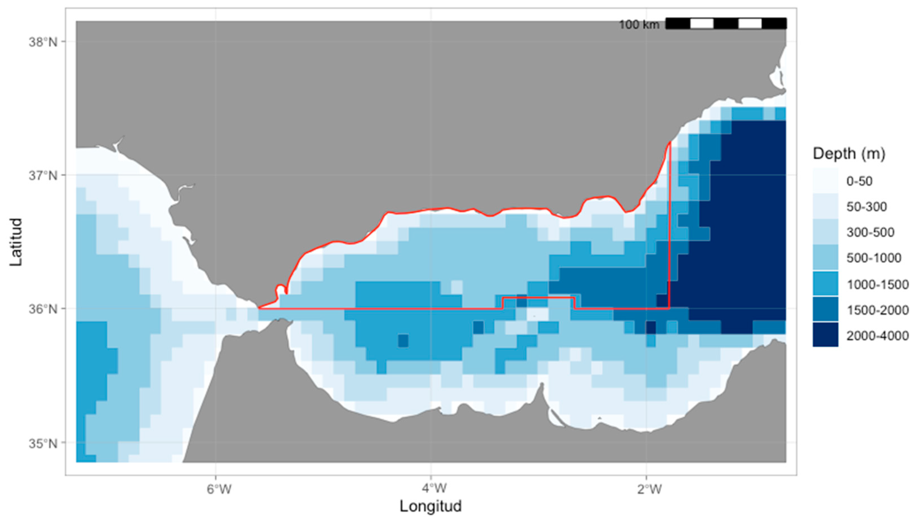
2.1. Study Area
2.2. Experimental Design
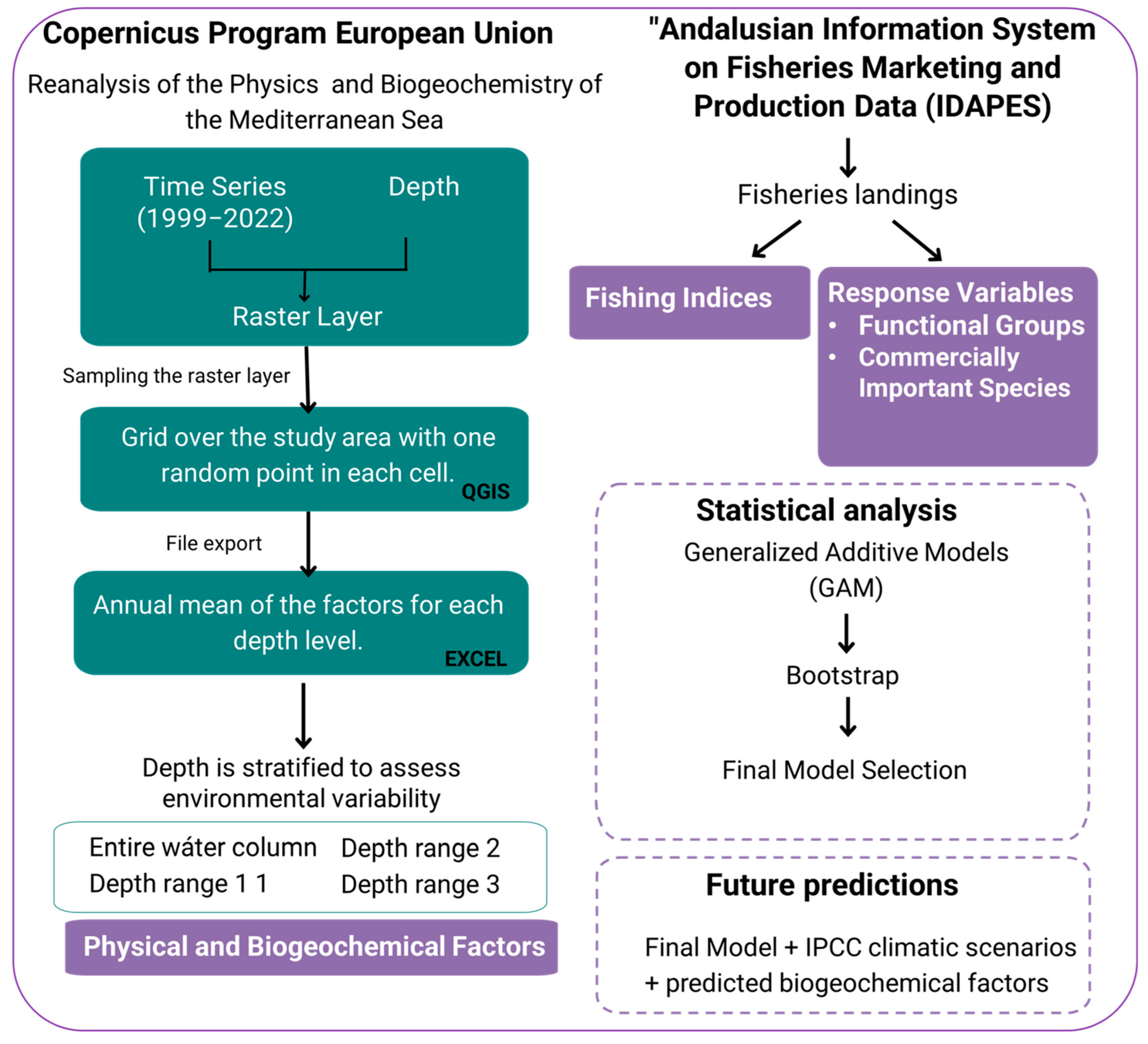
2.2.1. Geospatial Data Extraction and Processing
2.2.2. Fisheries in Andalusia
2.3. Statistical Analysis
- -
- Logarithm transformation: blue and red shrimp, horse mackerel, large pelagic fish, mackerel, Norway lobster and small pelagic fish.
- -
- Square root transformation: anchovies and deepwater rose shrimp.
2.4. Climate Change Scenarios and Projections
3. Results
3.1. Modelling
3.1.1. Functional Groups
- Benthic cephalopods
- Benthic Mollusks
- Decapods
- Large Pelagic Fish
- Small Pelagic Fish
3.1.2. Commercially Important Species and Groups
- Atlantic bonito
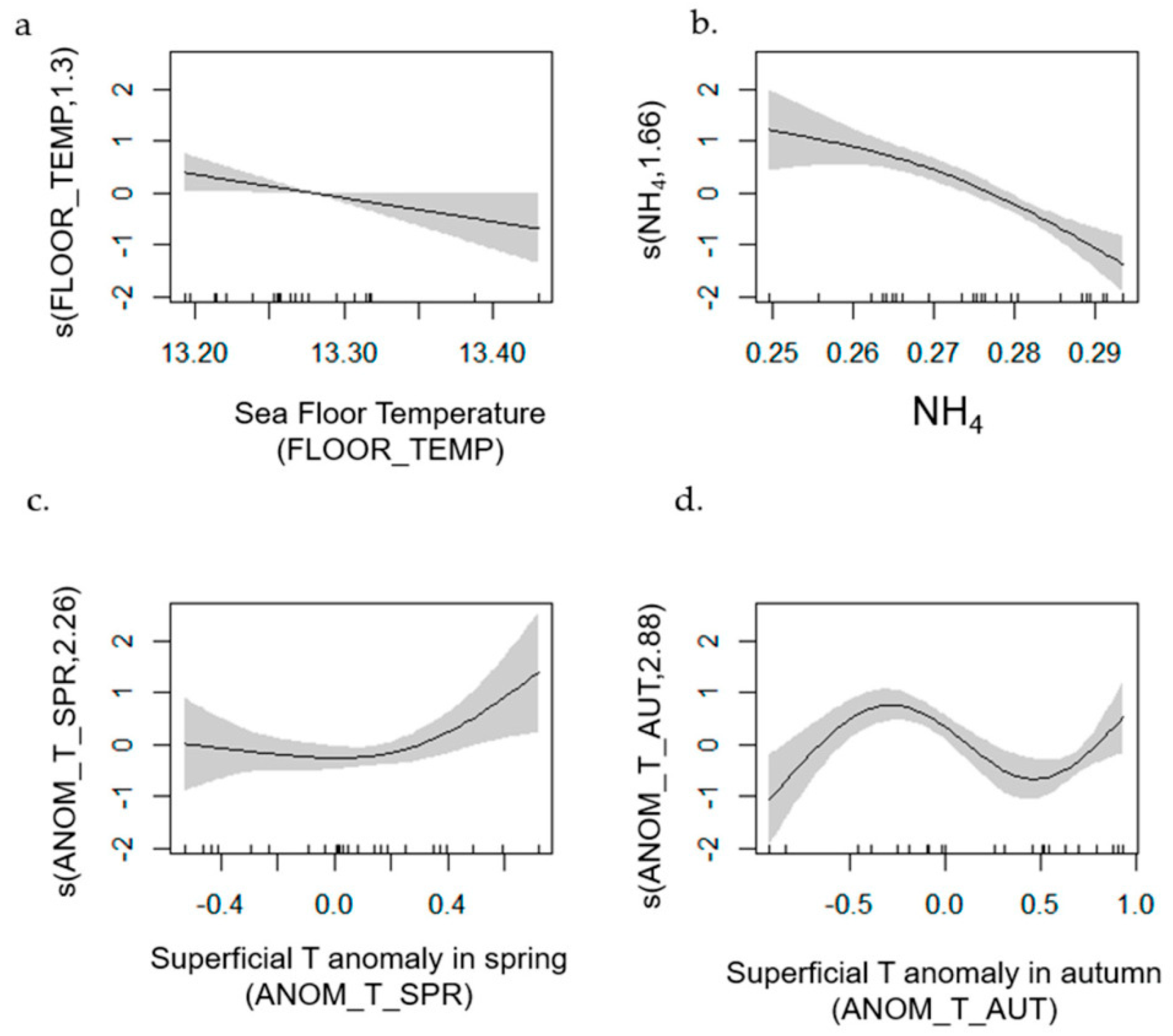
- Anchovy
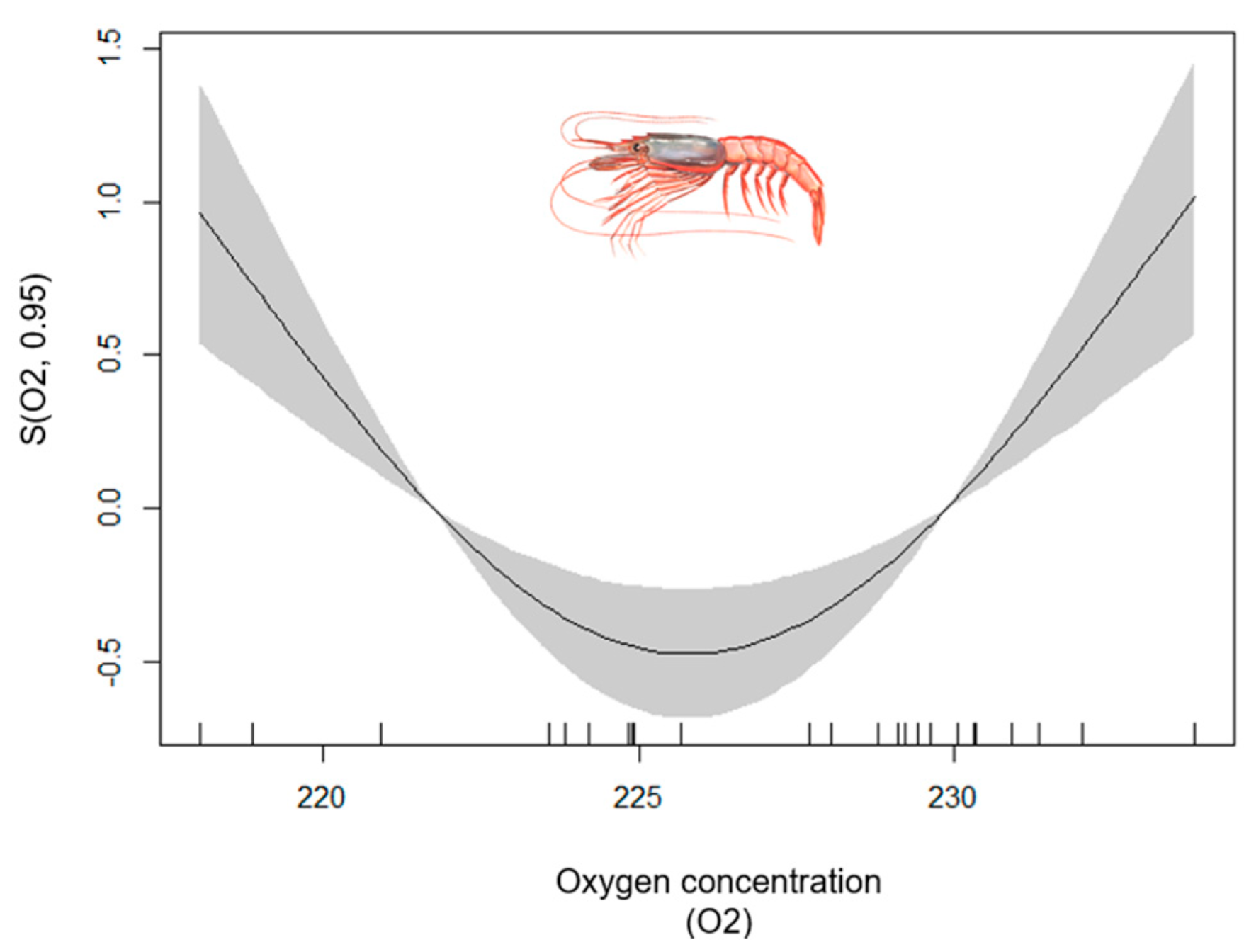
- Blue and red Shrimp
- Sardine
- Mackerel
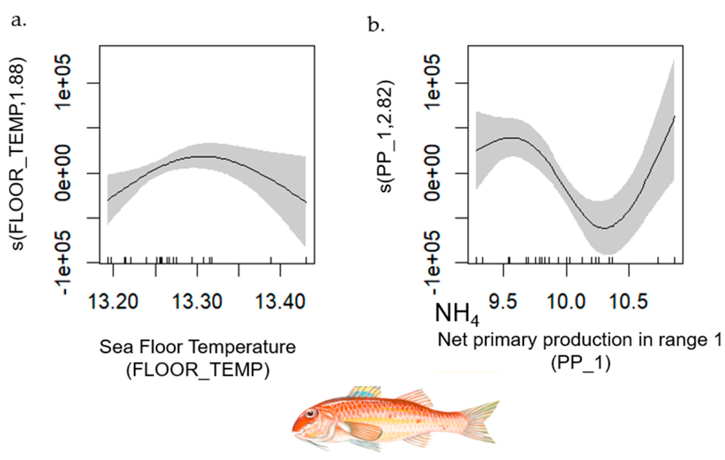
- Red Mullet
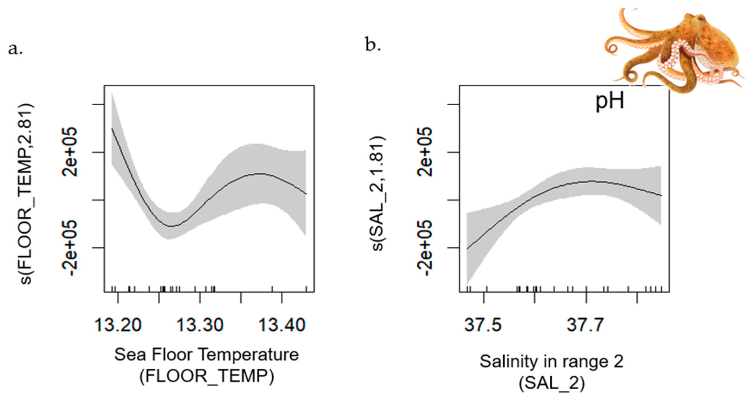
- Common Octopus
- Hake
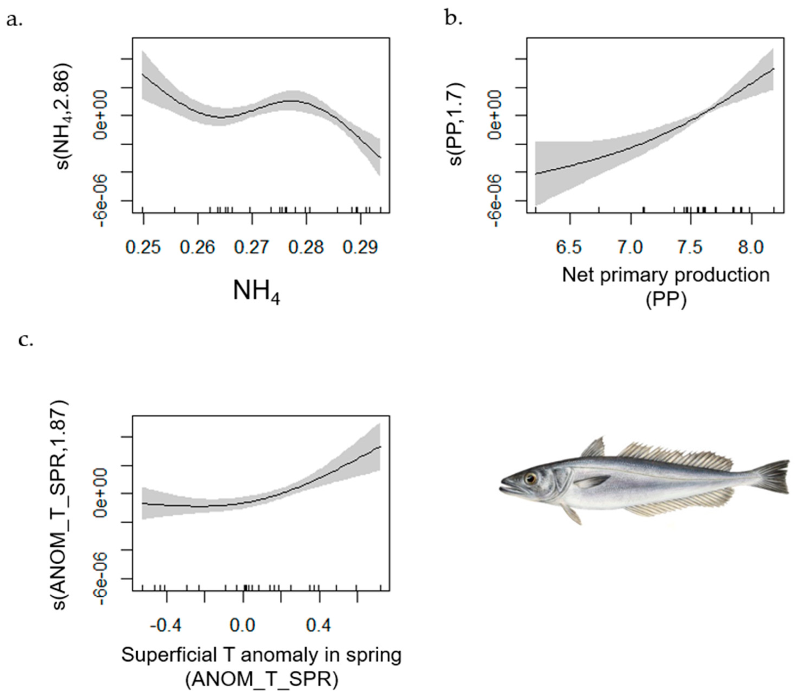
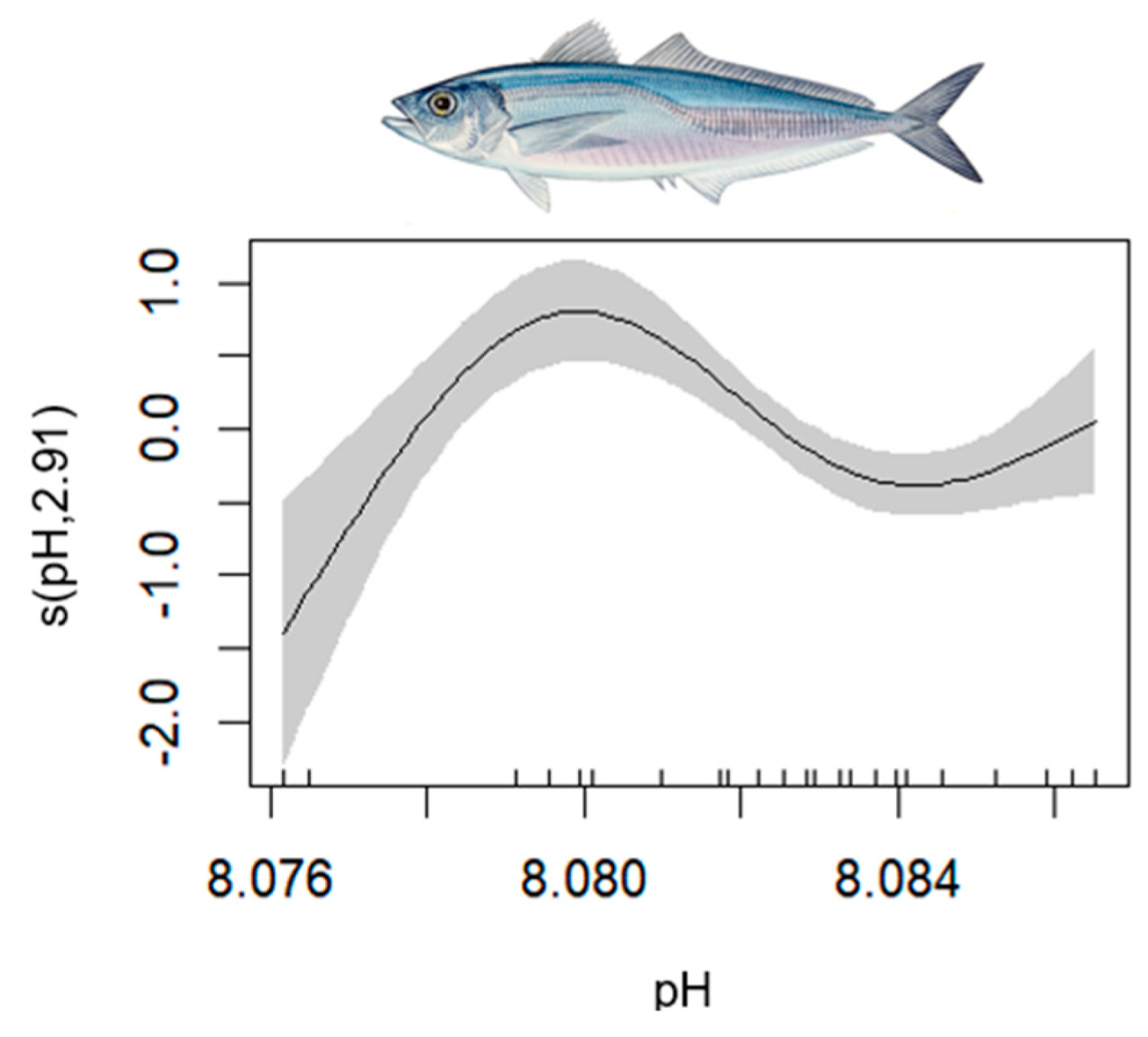
- Horse Mackerel
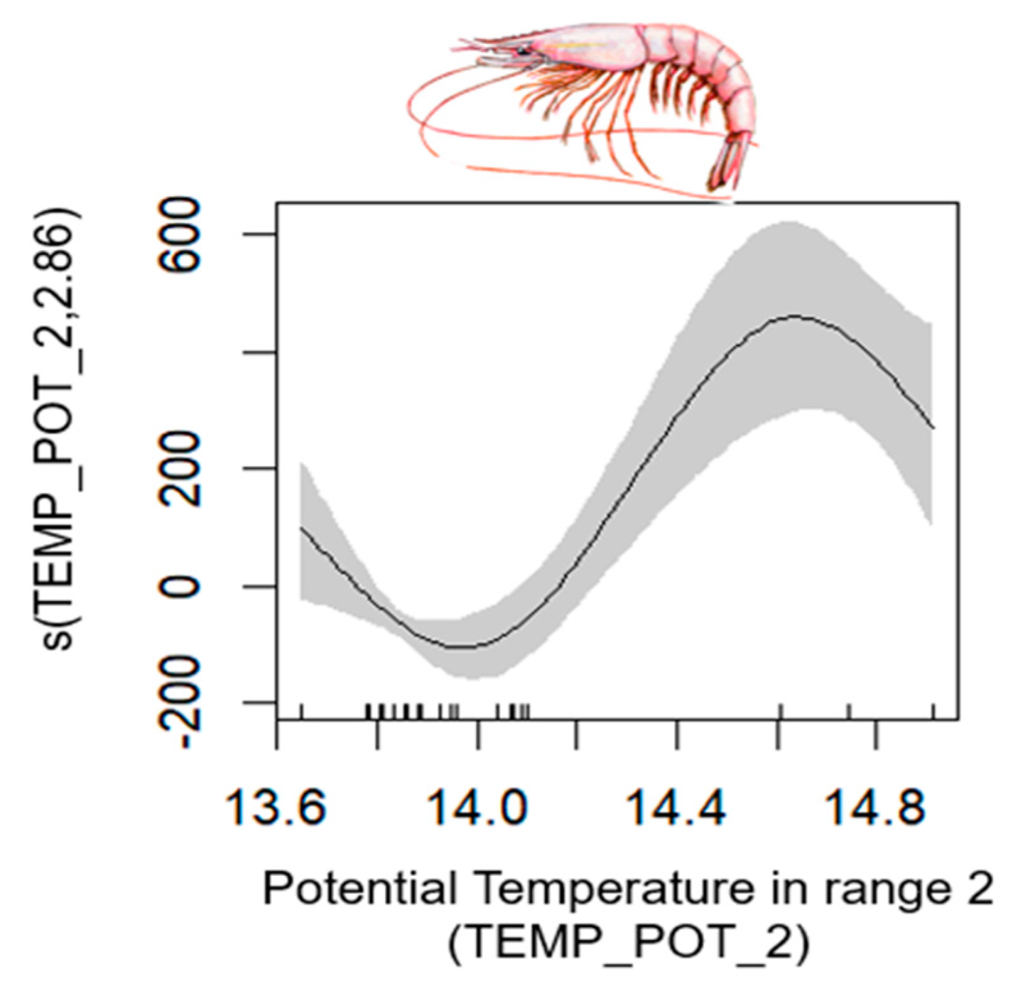
- Deepwater Rose Shrimp
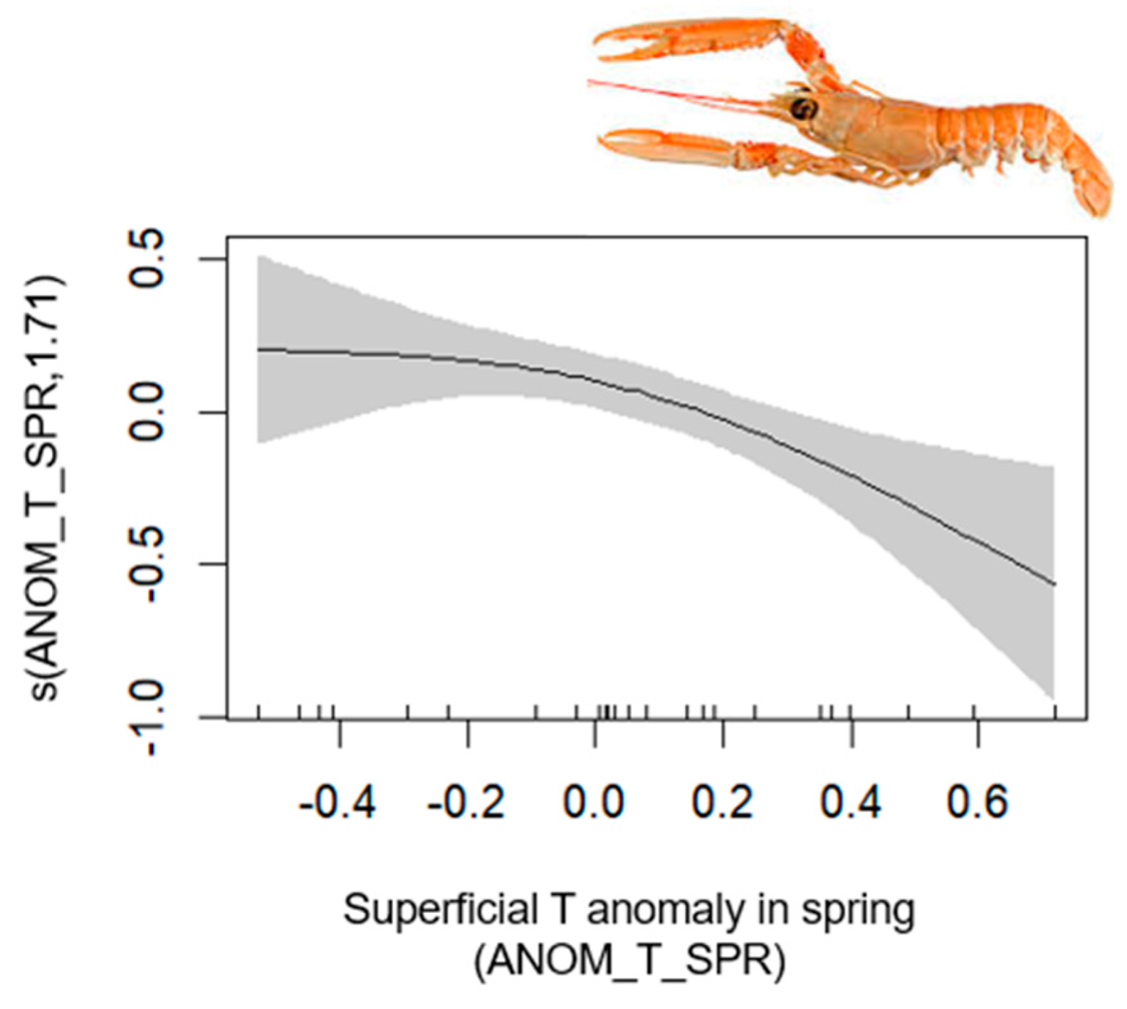
- Norway Lobster
3.2. Predictive Models with Climate Change Scenarios
4. Discussion
4.1. Fishing Impact
4.2. Environmental Impacts
4.3. Prediction Models
5. Conclusions
Supplementary Materials
Author Contributions
Funding
Data Availability Statement
Acknowledgments
Conflicts of Interest
References
- Pauly, D.; Christensen, V. Primary Production Required to Sustain Global Fisheries. Nature 1995, 374, 255–257. [Google Scholar] [CrossRef]
- Pauly, D.; Christensen, V.; Dalsgaard, J.; Froese, R.; Torres, F. Fishing Down Marine Food Webs. Science 1998, 279, 860–863. [Google Scholar] [CrossRef]
- Smith, C. Impact of Otter Trawling on an Eastern Mediterranean Commercial Trawl Fishing Ground. ICES J. Mar. Sci. 2000, 57, 1340–1351. [Google Scholar] [CrossRef]
- Frau, A.G. Sobrepesca y Artes Destructivas En El Mediterráneo. Problemática y Futuro de La Pesca. In Proceedings of the II Debates Sobre Economía Almeriense; Instituto de Estudios Almerienses: Almería, Spain, 1996. [Google Scholar]
- FAO. Code of Conduct for Responsible Fisheries; Food and Agriculture Organization of the United Nations: Rome, Italy, 1995; ISBN 9789251038345. [Google Scholar]
- FAO. The State of World Fisheries and Aquaculture 2020; FAO: Rome, Italy, 2020; ISBN 9789251326923. [Google Scholar]
- Sea Around Us. Marine Ecoregion: Western Mediterranean–Catch Data by Taxon. Available online: www.seaaroundus.org/data/#/meow/80?chart=catch-chart&dimension=taxon&measure=tonnage&limit=10 (accessed on 24 May 2023).
- González-Laxe, F. Estructura del Consumo de Pescado en España. Una Reducción de la Demanda y del Gasto. Boletin Econ. ICE 2018, 3105, 51–57. [Google Scholar] [CrossRef]
- Giráldez, A. Small Pelagic Resources: A Historic Perspective and Current State of the Resources. In Alboran Sea-Ecosystems and Marine Resources; Báez, J.C., Vázquez, J.-T., Camiñas, J.A., Malouli Idrissi, M., Eds.; Springer International Publishing: Cham, Switzerland, 2021; pp. 559–576. ISBN 9783030655150. [Google Scholar]
- Baro Domínguez, J.; García Jiménez, T.; Serna Quintero, J.M. Description of Artisanal Fisheries in Northern Alboran Sea. In Alboran Sea-Ecosystems and Marine Resources; Báez, J.C., Vázquez, J.-T., Camiñas, J.A., Malouli Idrissi, M., Eds.; Springer International Publishing: Cham, Switzerland, 2021; pp. 521–542. ISBN 9783030655150. [Google Scholar]
- García, A.; Laíz-Carrión, R.; Cortés, D.; Quintanilla, J.; Uriarte, A.; Ramírez, T.; Yebra, L.; Mercado, J.M.; García-Gómez, C.; Sammartino, S.; et al. Evolving from Fry Fisheries to Early Life Research on Pelagic Fish Resources. In Alboran Sea-Ecosystems and Marine Resources; Báez, J.C., Vázquez, J.-T., Camiñas, J.A., Malouli Idrissi, M., Eds.; Springer International Publishing: Cham, Switzerland, 2021; pp. 489–519. ISBN 9783030655150. [Google Scholar]
- Sea Around Us. Real 2019 Value (US$) by Taxon in the Waters of Alboran Sea. Available online: https://www.seaaroundus.org/data/#/meow/80?chart=catch-chart&dimension=taxon&measure=value&limit=10 (accessed on 24 May 2023).
- Cury, P.; Roy, C. Optimal Environmental Window and Pelagic Fish Recruitment Success in Upwelling Areas. Can. J. Fish. Aquat. Sci. 1989, 46, 670–680. [Google Scholar] [CrossRef]
- Van der Lingen, C.; Bertrand, A.; Bode, A.; Brodeur, R.; Cubillos, L.; Espinoza, P.; Friedland, K.; Garrido, S.; Irigoien, X.; Miller, T.; et al. Trophic Dynamics of Small Pelagic Fish. In Synthesis Book of the Program “Small Pelagic Fish and Climate Change Program (SPACC); Cambridge University Press: Cambridge, UK, 2009; pp. 333–403. [Google Scholar]
- Lanz, E.; Martinez, J.; Nevarez Martinez, M.; Dworak, J.A. Small Pelagic Fish Catches in the Gulf of California Associated with Sea Surface Temperature and Chlorophyll. Calif. Coop. Ocean. Fish. Investig. Rep. 2009, 50, 134–146. [Google Scholar]
- Bakun, A. Wasp-Waist Populations and Marine Ecosystem Dynamics: Navigating the “Predator Pit” Topographies. Prog. Oceanogr. 2006, 68, 271–288. [Google Scholar] [CrossRef]
- Fauchald, P.; Skov, H.; Skern-Mauritzen, M.; Johns, D.; Tveraa, T. Wasp-Waist Interactions in the North Sea Ecosystem. PLoS ONE 2011, 6, e22729. [Google Scholar] [CrossRef] [PubMed]
- Pennino, M.G.; Coll, M.; Albo-Puigserver, M.; Fernández-Corredor, E.; Steenbeek, J.; Giráldez, A.; González, M.; Esteban, A.; Bellido, J.M. Current and Future Influence of Environmental Factors on Small Pelagic Fish Distributions in the Northwestern Mediterranean Sea. Front. Mar. Sci. 2020, 7, 622. [Google Scholar] [CrossRef]
- Ottersen, G.; Alheit, J.; Drinkwater, K.; Friedland, K.; Hagen, E.; Stenseth, N.C. The Response of Fish Populations to Ocean Climate Fluctuations. In Marine Ecosystems and Climate Variation: The North Atlantic: A Comparative Perspective; Oxford University Press: Oxford, UK, 2004; pp. 73–94. [Google Scholar]
- Lejeusne, C.; Chevaldonné, P.; Pergent-Martini, C.; Boudouresque, C.F.; Pérez, T. Climate Change Effects on a Miniature Ocean: The Highly Diverse, Highly Impacted Mediterranean Sea. Trends Ecol. Evol. 2010, 25, 250–260. [Google Scholar] [CrossRef]
- Schickele, A.; Goberville, E.; Leroy, B.; Hattab, T.; Francour, P.; Raybaud, V. European small pelagic fish distribution under global change scenarios. Fish Fish. 2021, 22, 212–225. [Google Scholar] [CrossRef]
- Doray, M.; Petitgas, P.; Huret, M.; Duhamel, E.; Romagnan, J.B.; Authier, M.; Dupuy, C.; Spitz, J. Monitoring Small Pelagic Fish in the Bay of Biscay Ecosystem, Using Indicators from an Integrated Survey. Prog. Oceanogr. 2018, 166, 168–188. [Google Scholar] [CrossRef]
- Chaikin, S.; Dubiner, S.; Belmaker, J. Cold-water Species Deepen to Escape Warm Water Temperatures. Global Ecol. Biogeogr. 2022, 31, 75–88. [Google Scholar] [CrossRef]
- Parry, M.L. Assessment of Potential Effects and Adaptations for Climate Change in Europe: The Europe ACACIA Project; University of East Anglia, School of Environmental Sciences, Jackson Environment Institute: Norwich, UK, 2000. [Google Scholar]
- Vargas-Yáñez, M.; Garcia-Martinez, M.; Moya Ruiz, F.; López-Jurado, J.; Serra, M.; Balbín, R.; Santiago, R.; Salat, J.; Pasqual, J.; Ramírez, T.; et al. El Estado Actual de los Ecosistemas Marinos en el Mediterráneo Español en un Contexto de Cambio Climático; Instituto Español de Oceanografía: Madrid, Spain, 2019; ISBN 696-19-002-X. [Google Scholar]
- van Rijn, I.; Buba, Y.; DeLong, J.; Kiflawi, M.; Belmaker, J. Large but Uneven Reduction in Fish Size across Species in Relation to Changing Sea Temperatures. Glob. Change Biol. 2017, 23, 3667–3674. [Google Scholar] [CrossRef] [PubMed]
- Shapiro Goldberg, D.; Van Rijn, I.; Kiflawi, M.; Belmaker, J. Decreases in Length at Maturation of Mediterranean Fishes Associated with Higher Sea Temperatures. ICES J. Mar. Sci. 2019, 76, 946–959. [Google Scholar] [CrossRef]
- Bristow, L.A.; Mohr, W.; Ahmerkamp, S.; Kuypers, M.M.M. Nutrients That Limit Growth in the Ocean. Curr. Biol. 2017, 27, R474–R478. [Google Scholar] [CrossRef] [PubMed]
- Jaworski, N.A. Sources of Nutrients and the Scale of Eutrophication Problems in Estuaries. In Estuaries and Nutrients; Neilson, B.J., Cronin, L.E., Eds.; Humana Press: Totowa, NJ, USA, 1981; pp. 83–110. ISBN 9781461258261. [Google Scholar]
- Suárez-de Vivero, J.L.; Rodríguez-Mateos, J.C.; M’ Rabet-Temsamani, R. Regional Context and Maritime Governance. In Alboran Sea-Ecosystems and Marine Resources; Báez, J.C., Vázquez, J.-T., Camiñas, J.A., Malouli Idrissi, M., Eds.; Springer International Publishing: Cham, Switzerland, 2021; pp. 11–30. ISBN 9783030655167. [Google Scholar]
- Báez, J.C.; Vázquez, J.-T.; Camiñas, J.A.; Malouli Idrissi, M. (Eds.) Alboran Sea-Ecosystems and Marine Resources; Springer International Publishing: Cham, Switzerland, 2021; ISBN 9783030655150. [Google Scholar]
- Peel, M.C.; Finlayson, B.L.; McMahon, T.A. Updated World Map of the Köppen-Geiger Climate Classification. Hydrol. Earth Syst. Sci. 2007, 11, 1633–1644. [Google Scholar] [CrossRef]
- Sánchez-Laulhé, J.; Jansa, A.; Jiménez, C. Alboran Sea Area Climate and Weather. In Alboran Sea-Ecosystems and Marine Resources; Springer: Cham, Switzerland, 2021; pp. 31–83. ISBN 978-3-030-65515-0. [Google Scholar]
- Seager, R.; Liu, H.; Henderson, N.; Simpson, I.; Kelley, C.; Shaw, T.; Kushnir, Y.; Ting, M. Causes of Increasing Aridification of the Mediterranean Region in Response to Rising Greenhouse Gases. J. Clim. 2014, 27, 4655–4676. [Google Scholar] [CrossRef]
- Díaz, G.V.; Gárate-Lizarraga, I. Distribution of Functional Groups of Phytoplankton in the Euphotic Zone during an Annual Cycle in Bahía de La Paz, Gulf of California. CICIMAR Oceánides 2018, 33, 47–61. [Google Scholar] [CrossRef]
- Iglesias, I.; Lorenzo, M.N.; Gómez-Gesteira, M.; Taboada, J.J. La Temperatura Superficial Del Mar Como Herramienta de Predicción Climática. Av. Cienc. Tierra 2010, 11, 95–108. [Google Scholar]
- Coll, M.; Palomera, I.; Tudela, S.; Sardà, F. Trophic Flows, Ecosystem Structure and Fishing Impacts in the South Catalan Sea, Northwestern Mediterranean. J. Mar. Syst. 2005, 59, 63–96. [Google Scholar] [CrossRef]
- Hernández-Urcera, J.; Guerra, A. La Vida En Las Grandes Profundidades. Dendra Médica 2014, 13, 34–48. [Google Scholar]
- Dauvin, J.-C.; Iglesias, A.; Lorgere, J.-C. Circalittoral Suprabenthic Coarse Sand Community from the Western English Channel. J. Mar. Biol. Assoc. UK 1994, 74, 543–562. [Google Scholar] [CrossRef]
- Cifuentes Lemus, J.L.; Torres García, M.d.P.; Frías Mondragón, M. El Océano y sus Recursos; La Ciencia Desde México, 1st ed.; Fondo de Cultura Economica: Mexico City, Mexico, 1986; ISBN 9789681623883. [Google Scholar]
- N.O.A.A. What Are Pelagic Fish? Available online: https://oceanservice.noaa.gov/facts/pelagic.html (accessed on 16 July 2025).
- Nelson, J.S. Fishes of the World, 3rd ed.; J. Wiley: New York, NY, USA, 1994; ISBN 9780471547136. [Google Scholar]
- Torres, M.Á.; Coll, M.; Heymans, J.J.; Christensen, V.; Sobrino, I. Food-Web Structure of and Fishing Impacts on the Gulf of Cadiz Ecosystem (South-Western Spain). Ecol. Model. 2013, 265, 26–44. [Google Scholar] [CrossRef]
- Froese, R.; Pauly, D. (Eds.) FishBase 2000: Concepts, Design and Data Sources; ICLARM: Los Baños, Philippines, 2000; 344p. [Google Scholar]
- González Aguilar, M.; García Ruiz, C.; García Jiménez, T.; Serna Quintero, J.M.; Ciércoles Antonell, C.; Baro Domínguez, J. Demersal Resources. In Alboran Sea-Ecosystems and Marine Resources; Báez, J.C., Vázquez, J.-T., Camiñas, J.A., Malouli Idrissi, M., Eds.; Springer International Publishing: Cham, Switzerland, 2021; pp. 589–628. ISBN 9783030655167. [Google Scholar]
- Libralato, S.; Coll, M.; Tudela, S.; Palomera, I.; Pranovi, F. Quantifying Ecosystem Overfishing with a New Index of Fisheries’ Impact on Marine Trophic Webs. In Proceedings of the ICES-CIEM International Council for the Exploration of the Sea Annual Science Conference, Aberdeen, UK, 20 September 2005; Volume 2024. [Google Scholar]
- Pauly, D.; Watson, R. Background and Interpretation of the ‘Marine Trophic Index’ as Measure of Biodiversity. Philos. Trans. R. Soc. London. Ser. B Biol. Sci. 2005, 360, 415–423. [Google Scholar] [CrossRef]
- Branch, T.A.; Watson, R.; Fulton, E.A.; Jennings, S.; McGilliard, C.R.; Pablico, G.T.; Ricard, D.; Tracey, S.R. The Trophic Fingerprint of Marine Fisheries. Nature 2010, 468, 431–435. [Google Scholar] [CrossRef]
- Cohen, J. Statistical Power Analysis for the Behavioral Sciences; Routledge: London, UK, 2013; ISBN 9781134742707. [Google Scholar]
- Hastie, T.; Tibshirani, R. Generalized Additive Models: Some Applications. J. Am. Stat. Assoc. 1987, 82, 371–386. [Google Scholar] [CrossRef]
- O’Brien, K.; Garibaldi, L.; Agrawal, A.; Bennett, E.; Biggs, O.; Calderón Contreras, R.; Carr, E.; Frantzeskaki, N.; Gosnell, H.; Gurung, J.; et al. Thematic Assessment Report on the Underlying Causes of Biodiversity Loss and the Determinants of Transformative Change and Options for Achieving the 2050 Vision for Biodiversity of the Intergovernmental Science-Policy Platform on Biodiversity and Ecosystem Services; IPBES Secretariat: Bonn, Germany, 2024. [Google Scholar] [CrossRef]
- Soto-Navarro, J.; Jordà, G.; Amores, A.; Cabos Narvaez, W.D.; Somot, S.; Sevault, F.; Macías, D.; Djurdjevic, V.; Sannino, G.; Li, L.; et al. Evolution of Mediterranean Sea Water Properties under Climate Change Scenarios in the Med-CORDEX Ensemble. Clim. Dyn. 2020, 54, 2135–2165. [Google Scholar] [CrossRef]
- Reale, M.; Cossarini, G.; Lazzari, P.; Lovato, T.; Bolzon, G.; Masina, S.; Solidoro, C.; Salon, S. Acidification, Deoxygenation, and Nutrient and Biomass Declines in a Warming Mediterranean Sea. Biogeosciences 2022, 19, 4035–4065. [Google Scholar] [CrossRef]
- Colloca, F.; Scarcella, G.; Libralato, S. Recent Trends and Impacts of Fisheries Exploitation on Mediterranean Stocks and Ecosystems. Front. Mar. Sci. 2017, 4, 244. [Google Scholar] [CrossRef]
- Cone, R.S. The Need to Reconsider the Use of Condition Indices in Fishery Science. Trans. Am. Fish. Soc. 1989, 118, 510–514. [Google Scholar] [CrossRef]
- Tudela, S.; Coll, M.; Palomera, I. Developing an Operational Reference Framework for Fisheries Management on the Basis of a Two-Dimensional Index of Ecosystem Impact. ICES J. Mar. Sci. 2005, 62, 585–591. [Google Scholar] [CrossRef]
- Coll, M.; Libralato, S.; Tudela, S.; Palomera, I.; Pranovi, F. Ecosystem Overfishing in the Ocean. PLoS ONE 2008, 3, e3881. [Google Scholar] [CrossRef] [PubMed]
- Sabatés, A.; Martín, P.; Lloret, J.; Raya, V. Sea Warming and Fish Distribution: The Case of the Small Pelagic Fish, Sardinella Aurita, in the Western Mediterranean. Glob. Change Biol. 2006, 12, 2209–2219. [Google Scholar] [CrossRef]
- Giráldez, A.; Abad Moyano, R. Aspects on the reproductive biology of the Western Mediterranean anchovy from the coasts of Málaga (Alboran Sea). Sci. Mar. 1995, 59, 15–23. [Google Scholar]
- García, A.; Cortés, D.; Ramírez, T.; Giráldez, A.; Carpena, Á. Contribution of Larval Growth Rate Vairability to the Recruitment of the Bay of Málaga Anchovy (SW Mediterranean) during 2000–2001 Spawning Seasons. Sci. Mar. 2003, 67, 477–490. [Google Scholar] [CrossRef]
- Caballero-Huertas, M.; Vargas-Yánez, M.; Frigola-Tepe, X.; Viñas, J.; Muñoz, M. Unravelling the Drivers of Variability in Body Condition and Reproduction of the European Sardine along the Atlantic-Mediterranean Transition. Mar. Environ. Res. 2022, 179, 105697. [Google Scholar] [CrossRef]
- Ramírez, T.; Cortés, D.; García, A.; Carpena, A. Seasonal Variations of RNA/DNA Ratios and Growth Rates of the Alboran Sea Sardine Larvae (Sardina pilchardus). Fish. Res. 2004, 68, 57–65. [Google Scholar] [CrossRef]
- Frigola-Tepe, X.; Ollé-Vilanova, J.; Schull, Q.; Caballero-Huertas, M.; Viñas, J.; Muñoz, M. Phenotypic Plasticity in the Health Status of Western Mediterranean Sardines. Estimation of Spawning Quantity and Quality. Front. Mar. Sci. 2025, 12, 1576148. [Google Scholar] [CrossRef]
- Schickele, A.; Francour, P.; Raybaud, V. European Cephalopods Distribution under Climate-Change Scenarios. Sci. Rep. 2021, 11, 3930. [Google Scholar] [CrossRef]
- Márquez, L.; Larson, M.; Almansa, E. Effects of Temperature on the Rate of Embryonic Development of Cephalopods in the Light of Thermal Time Applied to Aquaculture. Rev. Aquac. 2021, 13, 706–718. [Google Scholar] [CrossRef]
- André, J.; Haddon, M.; Pecl, G.T. Modelling Climate-change-induced Nonlinear Thresholds in Cephalopod Population Dynamics. Glob. Change Biol. 2010, 16, 2866–2875. [Google Scholar] [CrossRef]
- Correll, D. Phosphorus: A Rate Limiting Nutrient in Surface Waters. Poult. Sci. 1999, 78, 674–682. [Google Scholar] [CrossRef]
- Feyjoo, P.; Riera, R.; Felipe, B.C.; Skalli, A.; Almansa, E. Tolerance Response to Ammonia and Nitrite in Hatchlings Paralarvae of Octopus Vulgaris and Its Toxic Effects on Prey Consumption Rate and Chromatophores Activity. Aquacult. Int. 2011, 19, 193–204. [Google Scholar] [CrossRef]
- García-del-Hoyo, J.J.; Castilla-Espino, D. Fisheries Economics and Management Under the Impact of Human and Varying Marine Environmental Conditions in the Alboran Sea. In Alboran Sea-Ecosystems and Marine Resources; Báez, J.C., Vázquez, J.-T., Camiñas, J.A., Malouli Idrissi, M., Eds.; Springer International Publishing: Cham, Switzerland, 2021; pp. 749–774. ISBN 9783030655167. [Google Scholar]
- Báez, J.C. Is Climate Change Modifying the Behavior of Sea Turtles? The Particular Case of the Loggerhead Turtle in the Alboran Sea. Front. Mar. Sci. 2024, 11, 1379303. [Google Scholar] [CrossRef]
- Tittensor, D.P.; Novaglio, C.; Harrison, C.S.; Heneghan, R.F.; Barrier, N.; Bianchi, D.; Bopp, L.; Bryndum-Buchholz, A.; Britten, G.L.; Büchner, M.; et al. Next-Generation Ensemble Projections Reveal Higher Climate Risks for Marine Ecosystems. Nat. Clim. Change 2021, 11, 973–981. [Google Scholar] [CrossRef] [PubMed]
- Jones, M.C.; Cheung, W.W.L. Multi-Model Ensemble Projections of Climate Change Effects on Global Marine Biodiversity. ICES J. Mar. Sci. 2015, 72, 741–752. [Google Scholar] [CrossRef]
- Rogers-Bennett, L.; Catton, C.A. Cascading Impacts of a Climate-Driven Ecosystem Transition Intensifies Population Vulnerabilities and Fishery Collapse. Front. Clim. 2022, 4, 908708. [Google Scholar] [CrossRef]
- Liu, Y.; Luo, L.; Feng, Y.; Li, J.; Su, B.; Qiu, Z. Impact of Climate Change on Global Catches of Marine Fisheries from 1971 to 2020. J. Ocean. Limnol. 2025, 43, 996–1013. [Google Scholar] [CrossRef]
- Price, J.; Warren, R.; Forstenhäusler, N. Biodiversity Losses Associated with Global Warming of 1.5 to 4 °C above Pre-Industrial Levels in Six Countries. Clim. Change 2024, 177, 47. [Google Scholar] [CrossRef]
- Wudu, K.; Abegaz, A.; Ayele, L.; Ybabe, M. The Impacts of Climate Change on Biodiversity Loss and Its Remedial Measures Using Nature Based Conservation Approach: A Global Perspective. Biodivers. Conserv. 2023, 32, 3681–3701. [Google Scholar] [CrossRef]
- Habibullah, M.S.; Din, B.H.; Tan, S.-H.; Zahid, H. Impact of Climate Change on Biodiversity Loss: Global Evidence. Environ. Sci. Pollut. Res. 2022, 29, 1073–1086. [Google Scholar] [CrossRef]
- UNFCCC. The Paris Agreement Paris Climate Change Conference, November 2015. 2018. Available online: https://unfccc.int/sites/default/files/english_paris_agreement.pdf (accessed on 20 May 2025).
- Holsman, K.K.; Hazen, E.L.; Haynie, A.; Gourguet, S.; Hollowed, A.; Bograd, S.J.; Samhouri, J.F.; Aydin, K. Towards Climate Resiliency in Fisheries Management. ICES J. Mar. Sci. 2019, 76, 1368–1378. [Google Scholar] [CrossRef]
- Calbet, A. Future Ocean Resilience and Adaptation Strategies. In The Ocean of Today, the Legacy of Tomorrow: Navigating the Future of Marine Life and Ecosystems; Calbet, A., Ed.; Springer Nature: Cham, Switzerland, 2025; pp. 163–169. ISBN 9783031882715. [Google Scholar]
- Alcorlo, P.; García-Tiscar, S.; Vidal-Abarca, M.R.; Suárez-Alonso, M.L.; Checa, L.; Díaz, I. Exploring the Intricate Connections between the Influence of Fishing on Marine Biodiversity and Their Delivery of Ecological Services Driven by Different Management Frameworks. Coasts 2024, 4, 168–197. [Google Scholar] [CrossRef]
- Stokes, C.R.; Bamber, J.L.; Dutton, A.; DeConto, R.M. Warming of +1.5 °C Is Too High for Polar Ice Sheets. Commun. Earth Environ. 2025, 6, 351. [Google Scholar] [CrossRef]
- Warren, R.; Price, J.; Graham, E.; Forstenhaeusler, N.; VanDerWal, J. The Projected Effect on Insects, Vertebrates, and Plants of Limiting Global Warming to 1.5 °C Rather than 2 °C. Science 2018, 360, 791–795. [Google Scholar] [CrossRef]
- Hoegh-Guldberg, O.; Jacob, D.; Taylor, M.; Bindi, M.; Brown, S.; Camilloni, I. Impacts of 1.5 °C and 2.0 °C Global Warming on Natural and Human Systems. IPCC Special Report on Global Warming of 1.5 °C. 2018. Available online: https://www.ipcc.ch/sr15/ (accessed on 20 May 2025).
- Díaz, S.; Settele, J.; Brondizio, E.S.; Ngo, H.T.; Guèze, M.; Agard, J. Summary for Policymakers of the Global Assessment Report on Biodiversity and Ecosystem Services. IPBES Global Assessment. 2019. Available online: https://ipbes.net/global-assessment (accessed on 20 May 2025).
- Peck, M.A.; Alheit, J.; Bertrand, A.; Catalán, I.A.; Garrido, S.; Moyano, M.; Rykaczewski, R.R.; Takasuka, A.; van der Lingen, C.D. Small Pelagic Fish in the New Millennium: A Bottom-up View of Global Research Effort. Prog. Oceanogr. 2021, 191, 102494. [Google Scholar] [CrossRef]
- Sarre, A.; Demarcq, H.; Keenlyside, N.; Krakstad, J.-O.; El Ayoubi, S.; Jeyid, A.M.; Faye, S.; Mbaye, A.; Sidibeh, M.; Brehmer, P. Climate Change Impacts on Small Pelagic Fish Distribution in Northwest Africa: Trends, Shifts, and Risk for Food Security. Sci. Rep. 2024, 14, 12684. [Google Scholar] [CrossRef]
- Fabry, V.J.; Seibel, B.A.; Feely, R.A.; Orr, J.C. Impacts of Ocean Acidification on Marine Fauna and Ecosystem Processes. ICES J. Mar. Sci. 2008, 65, 414–432. [Google Scholar] [CrossRef]
- Whiteley, N.M. Physiological and ecological responses of crustaceans to ocean acidification. Mar. Ecol. Prog. Ser. 2011, 430, 257–271. [Google Scholar] [CrossRef]
- NOAA Fisheries. Ocean Futures Under Ocean Acidification, Marine Protection, and Changing Fishing Pressures Explored Using a Worldwide Suite of Ecosystem Models. Available online: https://www.fisheries.noaa.gov/resource/peer-reviewed-research/ocean-futures-under-ocean-acidification-marine-protection-and (accessed on 24 May 2025).
- Bastardie, F.; Feary, D.A.; Brunel, T.; Kell, L.T.; Döring, R.; Metz, S.; Eigaard, O.R.; Basurko, O.C.; Bartolino, V.; Bentley, J.; et al. Ten Lessons on the Resilience of the EU Common Fisheries Policy towards Climate Change and Fuel Efficiency-A Call for Adaptive, Flexible and Well-Informed Fisheries Management. Front. Mar. Sci. 2022, 9, 947150. [Google Scholar] [CrossRef]
- Rodriguez-Perez, A.; Tsikliras, A.C.; Gal, G.; Steenbeek, J.; Falk-Andersson, J.; Heymans, J.J. Using Ecosystem Models to Inform Ecosystem-Based Fisheries Management in Europe: A Review of the Policy Landscape and Related Stakeholder Needs. Front. Mar. Sci. 2023, 10, 1196329. [Google Scholar] [CrossRef]
- Pikitch, E.K.; Santora, C.; Babcock, E.A.; Bakun, A.; Bonfil, R.; Conover, D.O.; Dayton, P.; Doukakis, P.; Fluharty, D.; Heneman, B.; et al. Ecosystem-Based Fishery Management. Science 2004, 305, 346–347. [Google Scholar] [CrossRef] [PubMed]

| Common Name | Scientific Name | Ranges |
|---|---|---|
| Atlantic bonito | Sarda sarda (Bloch, 1793) | 1 |
| Anchovy | Engraulis encrasicolus (L., 1758) | 1 |
| Mackerel | Scomber spp. | 1 |
| Norway Lobster | Nephrops norvegicus (L. 1758) | 2, 3 |
| Deep-Water Rose Shrimp | Parapenaeus longirostris (Lucas, 1846) | 2, 3 |
| Blue and Red Shrimp | Aristeus antennatus (Risso, 1816) | 2, 3 |
| Horse mackerel | Trachurus spp. | 1 |
| Hake | Merluccius merluccius (L., 1758) | 2, 3 |
| Common octopus | Octopus vulgaris (Cuvier, 1797) | 2, 3 |
| Red mullet | Mullus barbatus (L., 1758) | 1, 2 |
| Sardine | Sardina pilchardus (Walbaum, 1792) | 1 |
| Species/Group | Depth Range (m) | R2 | (95% CI) | Significant Linear Predictors | Significant Non-Linear Predictor |
|---|---|---|---|---|---|
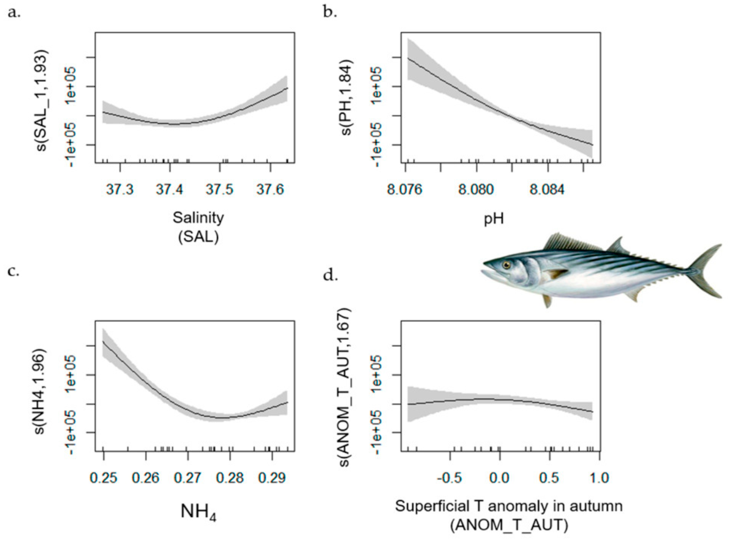
| Atlantic Bonito | 1–702 | 0.90 | [0.91, 1] | ANOM_T_SPR (−); FLOOR_TEMP (−); NO3 (−); CHL (+) | SAL; NH4; PH; MTI |
| Benthic Mollusks | 51–182 | 0.65 | [0.53, 0.87] | MTI (−); O2_2 (−); ANOM_SPR_2 (−) | |
| Blue and Red Shrimp | 1–702 | 0.71 | [0.63, 0.97] | MTI (+); FLOOR_TEMP (+); SAL (−); NH4 (+); ANOM_T_SPR (−); ANOM_T_AUT (−) | O2 |
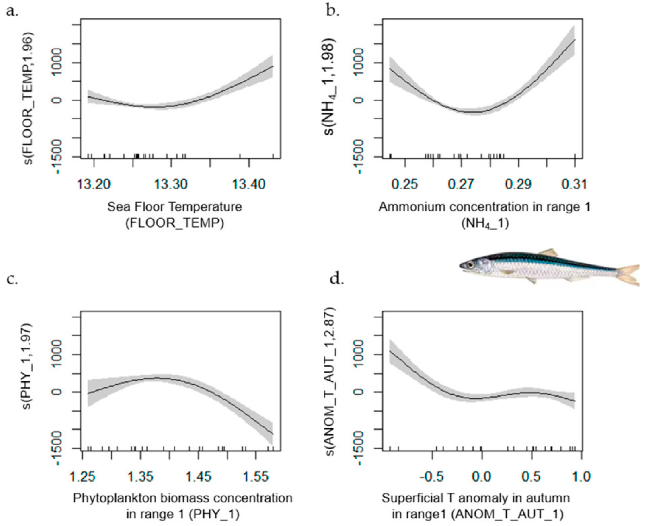
| Anchovy | 1–42 | 0.86 | [0.825, 1] | L index (−); SAL_1 (−); ANOM_T_SPR (−); ANOM_T_SUM (−) | FLOOR_TEMP; ANOM_T_AUT; NH4_1; PHY_1 |
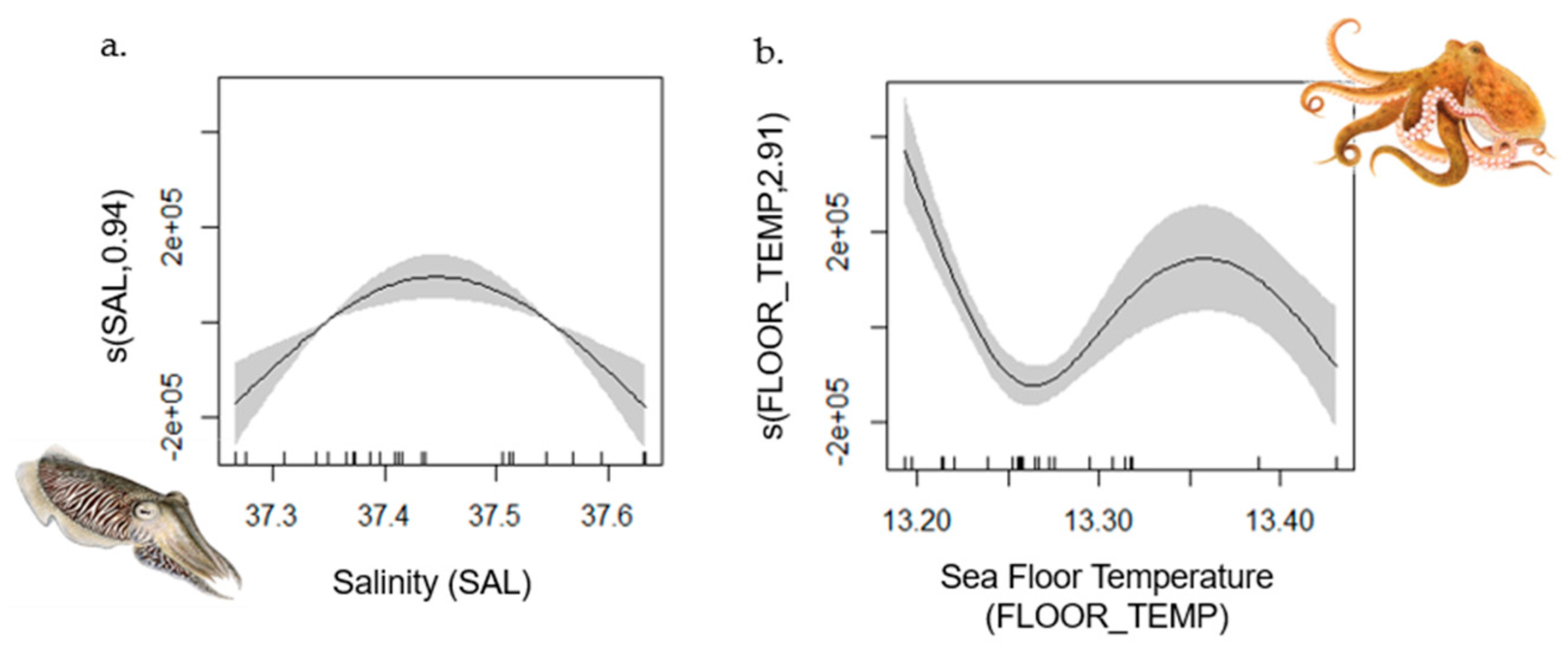
| Benthic Cephalopods | 1–702 | 0.77 | [0.58, 0.94] | ANOM_T_WIN (−) | FLOOR_TEMP; SAL |
| Decapods | 1–702 | 0.74 | [0.72, 0.98] | L index (−); MTI (−); FLOOR_TEMP (−); SAL (+); PH (−); ANOM_T_SPR (+); ANOM_T_AUT (+) | NH4 |
| Deepwater Rose Shrimp | 51–182 | 0.78 | [0.60, 0.96] | L index (−); CAR_2 (−) | TEMP_POT_2 |
| Hake | 1–702 | 0.75 | [0.71, 0.98] | MTI (−); ANOM_T_AUT (+); ANOM_T_SUM (+) | NH4; PP; ANOM_T_SPR |
| Horse Mackerel | 1–702 | 0.611 | [0.36, 0.93] | L index (+); SAL (−); PHY (+) | PH |
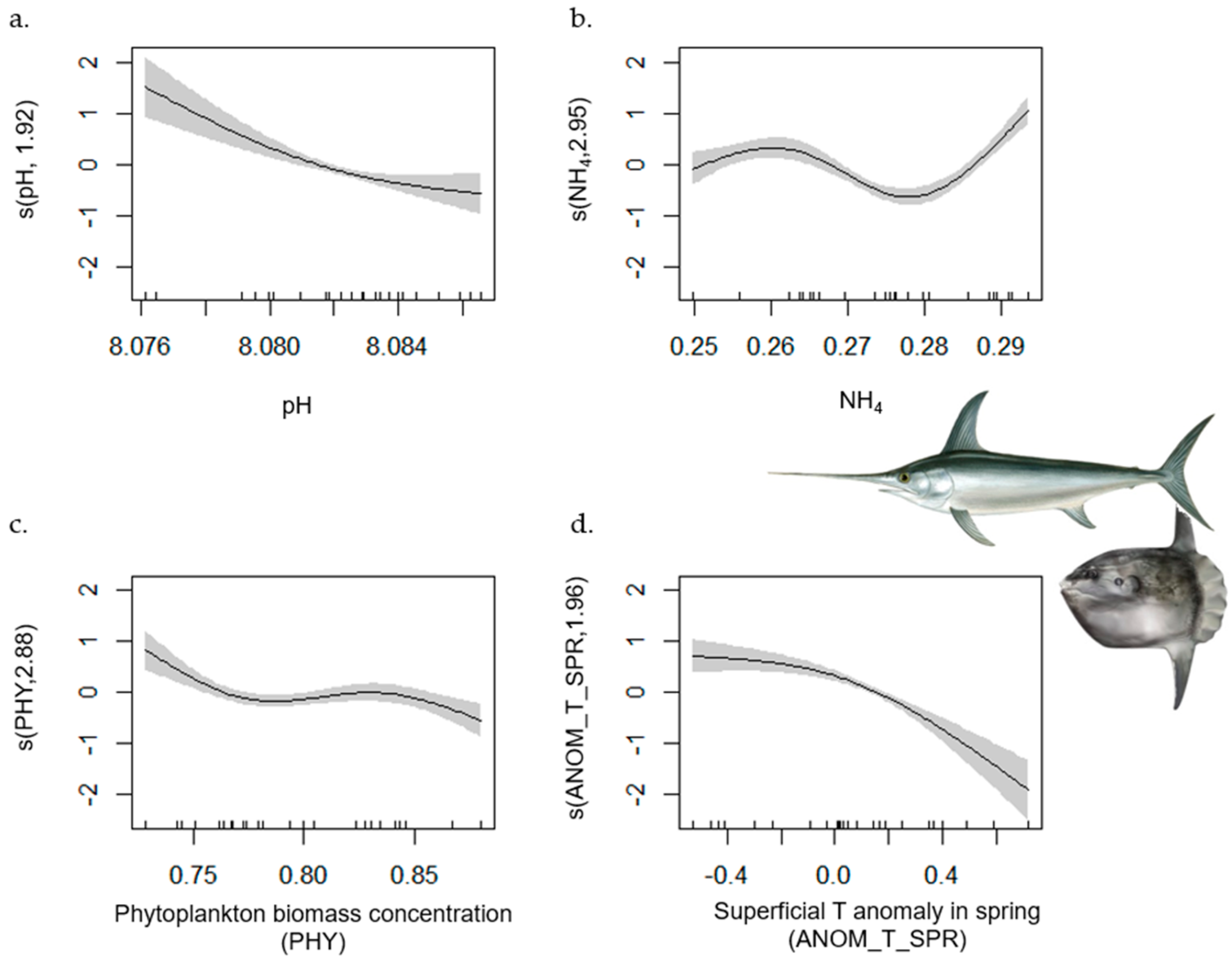
| Large Pelagic Fish | 1–702 | 0.82 | [0.72, 1] | MTI (+); SAL (−); NO3 (−); ANOM_T_SUM (−); ANOM_T_AUT (−) | NH4; ANOM_T_SPR; PHY; PH |
| Mackerels | 1–42 | 0.78 | [0.85, 1] | L index (−); ANOM_T_WIN (−); ANOM_T_SUM (−) | NH4; ANOM_T_AUT; ANOM_T_SPR |
| Norway lobster | 1–702 | 0.80 | [0.76, 0.98] | L index (+); SAL (−); NH4 (+); PHY (−); ANOM_T_WIN (−); ANOM_T_AUT (−) | ANOM_T_SPR |
| Common octopus | 51–182 | 0.65 | [0.44, 0.91] | MTI (+) | FLOOR_TEMP; SAL |
| Red Mullet | 1–42 | 0.726 | [0.70, 0.98] | MTI (+); O2_1 (−); NH4_1 (+) | PP_1; FLOOR_TEMP |
| Sardine | 1–702 | 0.80 | [0.72, 0.95] | PPR (+); CAR (−); CHL (+); ANOM_T_WIN (−); PH (+); ANOM_T_SPR (+); ANOM_T_AUT (+) | |
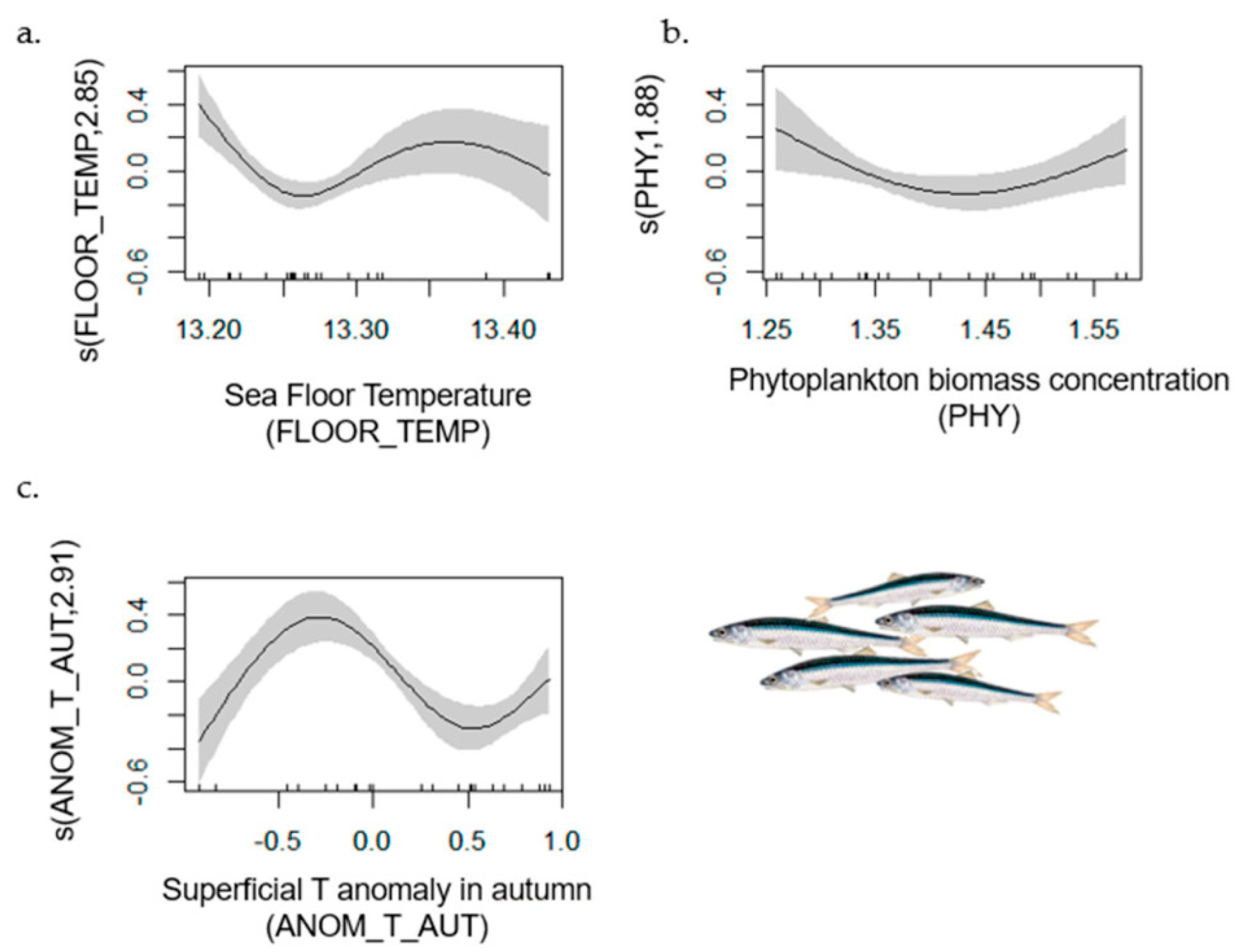
| Small Pelagic Fish | 1–42 | 0.75 | [0.71, 1] | NH4_1 (−); ANOM_T_WIN (−); ANOM_T_SUM (−) | FLOOR_TEMP; ANOM_T_AUT |
| Scenario | ANOM_T_WIN | ANOM_T_SPR | ANOM_T_SUM | ANOM_T_AUT | FLOOR_TEMP |
|---|---|---|---|---|---|
| Mitigation | 1.69 | 1.62 | 2.18 | 1.57 | 13.59 |
| Catastrophic | 2.78 | 2.71 | 3.27 | 2.66 | 13.64 |
| Species/Group | Mean Catch (kg) | Mitigation (+2 °C) | Trend | Catastrophic (+3.5 °C) | Trend |
|---|---|---|---|---|---|
| Blue and Red Shrimp | 258,878.00 | 101,296.70 | Decrease | 180,218.30 | Stable |
| Common Octopus | 924,241.35 | 55,004.66 | Decrease | 0 | Disappear |
| Deepwater Rose Shrimp | 211,640.83 | 0 | Disappear | 0 | Disappear |
| Hake | 434,068.01 | 43,618.55 | Decrease | 26,418.58 | Decrease |
| Norway Lobster | 76,078.61 | 0 | Disappear | 0 | Disappear |
| Red Mullet | 261,873.87 | 175,309.20 | Stable | 341,680.00 | Stable |
| Sardine | 5,235,253.91 | 0 | Disappear | 0 | Disappear |
| Benthic Cephalopods | 1,027,025.05 | 0 | Disappear | 0 | Disappear |
| Benthic Mollusks | 1,183,861.15 | 0 | Disappear | 0 | Disappear |
| Decapods | 520,997.38 | 41,101.05 | Decrease | 20,131.52 | Decrease |
Disclaimer/Publisher’s Note: The statements, opinions and data contained in all publications are solely those of the individual author(s) and contributor(s) and not of MDPI and/or the editor(s). MDPI and/or the editor(s) disclaim responsibility for any injury to people or property resulting from any ideas, methods, instructions or products referred to in the content. |
© 2025 by the authors. Licensee MDPI, Basel, Switzerland. This article is an open access article distributed under the terms and conditions of the Creative Commons Attribution (CC BY) license (https://creativecommons.org/licenses/by/4.0/).
Share and Cite
Uzategui, I.; Garcia-Tiscar, S.; Alcorlo, P. Exploring How Climate Change Scenarios Shape the Future of Alboran Sea Fisheries. Water 2025, 17, 2313. https://doi.org/10.3390/w17152313
Uzategui I, Garcia-Tiscar S, Alcorlo P. Exploring How Climate Change Scenarios Shape the Future of Alboran Sea Fisheries. Water. 2025; 17(15):2313. https://doi.org/10.3390/w17152313
Chicago/Turabian StyleUzategui, Isabella, Susana Garcia-Tiscar, and Paloma Alcorlo. 2025. "Exploring How Climate Change Scenarios Shape the Future of Alboran Sea Fisheries" Water 17, no. 15: 2313. https://doi.org/10.3390/w17152313
APA StyleUzategui, I., Garcia-Tiscar, S., & Alcorlo, P. (2025). Exploring How Climate Change Scenarios Shape the Future of Alboran Sea Fisheries. Water, 17(15), 2313. https://doi.org/10.3390/w17152313