Abstract
A mass abatement scalable system through managed aquifer recharge (MAR-MASS) improves mass extraction from groundwater with a variable-density flow. This method is superior to conventional injection systems because it promotes uniform mass displacement, reduces density gradients, and increases mass extraction efficiency over time. Simulations of various scenarios involving hydrogeologic variables, including hydraulic conductivity, vertical anisotropy, specific yield, mechanical dispersion, molecular diffusion, and mass concentration in aquifers, have identified critical variables and parameters influencing mass transport interactions to optimize the system. MAR-MASS is adaptable across hydrogeologic conditions in aquifers that are 25–75 m thick, comprising unconsolidated materials with hydraulic conductivities between 5 and 100 m/d. It is effective in scenarios near coastal areas or in aquifers with variable-density flows within the continent, with mass concentrations of salts or solutes ranging from 3.5 to 35 kg/m3. This system employs a modular approach that offers scalable and adaptable solutions for mass extraction at specific locations. The integration of programming tools, such as Python 3.13.2, along with technological strategies utilizing parallelization techniques and high-performance computing, has facilitated the development and validation of MAR-MASS in mass extraction with remarkable efficiency. This study confirmed the utility of these tools for performing calculations, analyzing information, and managing databases in hydrogeologic models. Combining these technologies is critical for achieving precise and efficient results that would not be achievable without them, emphasizing the importance of an advanced technological approach in high-level hydrogeologic research. By enhancing groundwater quality within a comparatively short time frame, expanding freshwater availability, and supporting sustainable aquifer recharge practices, MAR-MASS is essential for improving water resource management.
1. Introduction
Managed Aquifer Recharge (MAR) involves introducing water into aquifers for future use, offering significant environmental benefits [1]. This technique enhances groundwater supply and reinforces its role as a safeguard against fluctuations in surface water availability. With their substantial storage capacity, aquifers are ideal for subsurface storage, efficiently reducing evaporation and minimizing contamination by requiring less land area than surface reservoirs [1].
The successful implementation of MAR projects relies on factors such as site selection, availability of quality water, aquifer capacity to store and treat water, social acceptance, costs, and the necessary technical resources. Technologies such as Aquifer Storage and Recovery (ASR) and Aquifer Storage Transfer and Recovery (ASTR) can help address some of these challenges by enabling controlled recharge, which reduces the need for extensive surface infrastructure and minimizes contamination risks [1].
Groundwater naturally contains dissolved constituents due to the weathering of sediments and rocks, with concentrations that depend on the water’s residence time. However, human activities, such as agriculture and industry, have introduced additional compounds into groundwater [2,3,4], exacerbating the salinization of aquifers. The overexploitation of groundwater reduces freshwater recharge and increases the risk of saltwater intrusion [5]. Additionally, rock dissolution driven by geological conditions—raises salinity levels by releasing ions like sodium and calcium into the groundwater [6].
Saltwater intrusion, a form of aquifer salinization, is often worsened by excessive groundwater extraction, allowing saltwater to encroach into freshwater aquifers, particularly in coastal areas. To mitigate this intrusion, various solutions have been proposed based on the theoretical behavior of aquifers with different water densities, including positive, negative, mixed, and double-pumping hydraulic barriers [7].
The variability of the saltwater wedge within aquifers poses significant challenges for remediation techniques due to its spatial and temporal nature. A modular approach is proposed to effectively adapt the MAR system to each aquifer’s specific hydrodynamic and hydrogeological conditions. This scalable method employs three-dimensional modeling and a coupled injection and extraction module design. The effectiveness of the system was evaluated by measuring salt mass extraction per unit time and the residual salt mass concentration in the intervened area, considering factors such as salt concentration, hydraulic conductivity, vertical anisotropy, specific yield, mechanical dispersion, and molecular diffusion. Different scenarios were compared under hydrogeological conditions and hydrodynamic parameters to identify the most efficient configuration.
2. Materials and Methods
2.1. Conceptual Model
The methodological process began by creating a conceptual model of a prototype aquifer and describing its main characteristics and processes in the context of aquifers with an initial salt concentration. The resulting models combined different values within a range of possible values according to the material for the various hydrodynamic parameters analyzed, including hydraulic conductivity, vertical anisotropy, specific yield, mechanical dispersion, and molecular diffusion. This approach facilitates understanding and analysis by allowing simulations that combine different parameter values.
The implementation of the method aimed to analyze the behavior of mass transport and extraction in a free, homogeneous aquifer, with a thickness ranging from 25 to 75 m, composed of unconsolidated materials such as medium and coarse sand and a mixture of sand and gravel, considering the vertical anisotropy of hydraulic conductivity in the materials. A first-type boundary condition (Dirichlet) was imposed on the lateral surface area of the domain to set the groundwater level and mass concentration entering the system. Their values remained constant and were independent of inflow into the system. The center of the domain was the test well(s) simulating the injection and extraction of water according to the system configuration. The domain was cylindrical with a diameter of 7 km, ensuring that the boundary conditions did not disturb or influence the flow and mass transport by the well or the set of wells in the center of the domain. The model had no boundary conditions at its base or surface.
2.2. Modeling Approach
Identifying key variables led to the selection of specific numerical models suitable for analyzing aquifers. These models must accurately simulate relevant hydrogeologic processes, such as groundwater flow, mass transport, and the interaction between freshwater and saltwater. The selected numerical models defined parameters that significantly influenced the simulations. The description should cover various hydraulic characteristics of the aquifer, including hydraulic conductivity, vertical anisotropy of the hydraulic conductivity, specific yield, mechanical dispersion, and molecular diffusion under varying mass concentration values. The modeling scenarios defined these factors to evaluate the behavior of the aquifer under different conditions. Analysts ran simulations to analyze the behavior of an aquifer, after creating numerical models and outlining the parameters and modeling scenarios. This process includes comparing different scenarios, evaluating the effectiveness of the proposed strategies, and identifying possible areas of improvement in configuring the injection and extraction systems to maximize the efficiency of the method. The conceptual model provides the theoretical and conceptual basis for the modeling approach, which determines the specific techniques used to translate the conceptual model into a numerical model. This approach guides the selection of hydraulic parameters, the number of scenarios that must be simulated, and temporal and spatial (mesh) discretization, allowing adequate simulation of hydrogeologic system behavior.
2.2.1. Parameter Selection
Multiple scenarios were modeled to achieve optimal method efficiency. These included aquifers with various hydraulic parameters and applied boundary conditions to the prototype domain. The model included vertical anisotropy, specific storage, mechanical dispersion, and molecular diffusion, representing different aquifers. Table 1 summarizes the vital hydraulic parameters and initial conditions used in these scenarios, along with a set of selected values intended to represent the behavior of the aquifer under the predetermined hydrogeologic conditions. The values for hydraulic conductivity ranged from 5 to 100 m/d, vertical anisotropies ranged from 1 to 30, and aquifer initial salt concentrations ranged from 3.5 to 35 kg/m3, with different coefficients being considered for the effects of mechanical dispersion and molecular diffusion (Table 1).

Table 1.
Parameters and initial conditions used in numerical simulations.
Table 2 presents the specific yield (Sy) values based on hydraulic conductivity and material classification, employing four to five scenarios for each hydraulic conductivity value for a specific yield.
Table 2.
Specific yield values (Sy) based on material type and hydraulic conductivity (K).
Table 2.
Specific yield values (Sy) based on material type and hydraulic conductivity (K).
| Material | K (m/d) | Sy | ||||||
|---|---|---|---|---|---|---|---|---|
| 0.15 | 0.20 | 0.25 | 0.30 | 0.35 | ||||
| Sand and gravel | Medium sand | 5 | • | • | • | • | ||
| 10 | • | • | • | • | ||||
| Coarse Sand | 20 | • | • | • | • | • | ||
| 40 | • | • | • | • | ||||
| 60 | • | • | • | • | ||||
| 80 | • | • | • | • | ||||
| 100 | • | • | • | • | ||||
Note: Adapted from [8,9]. The symbol “•” indicates combinations of K and Sy values used in the simulation.
2.2.2. Number of Scenarios
Table 1 provides the values for four levels of vertical anisotropy, five for the initial concentration, and three for molecular diffusion, totaling 60 scenarios. Four mechanical dispersion values were defined for each component: longitudinal dispersivity in the horizontal direction, transverse dispersivity in the horizontal direction, and transverse dispersivity in the vertical direction. These considerations yielded 240 scenarios. Data from Table 2 provide an analysis of the hydraulic conductivity and specific yield, covering 29 scenarios ranging from 5 to 100 m/d; the multiplication of these 29 scenarios from Table 2 with the 240 scenarios from Table 1 resulted in 6950 scenarios.
2.2.3. Temporal Discretization
The simulation time for the proposed scenarios was 3000 days, which was selected to capture mass transport behavior across all scenarios. The temporal discretization at uniform intervals of 30 days contributes to understanding mass propagation and movement within the aquifer over time. The selected temporal discretization provided the desired precision corresponding to mass extraction in tons per month. This preserved the balance between the expected results and the computational time required for the calculations. Temporal discretization was linked to spatial discretization by dividing the domain into elements to calculate the flow and mass transport of each element during each time step.
2.2.4. Mesh Discretization
Mesh discretization involves dividing the aquifer domain into elements to better represent the geometry and properties of a subsurface medium. This step solves the mathematical equations describing aquifer water flow and mass transport. Vertical refinement uses 1-m-thick mathematical layers, resulting in numerical layers equivalent to the domain depth in meters. Horizontal refinement primarily utilizes triangular elements, whereas rectangular elements are employed for the principal axes (X, Y), dividing the domain into quadrants, as shown in Figure 1.
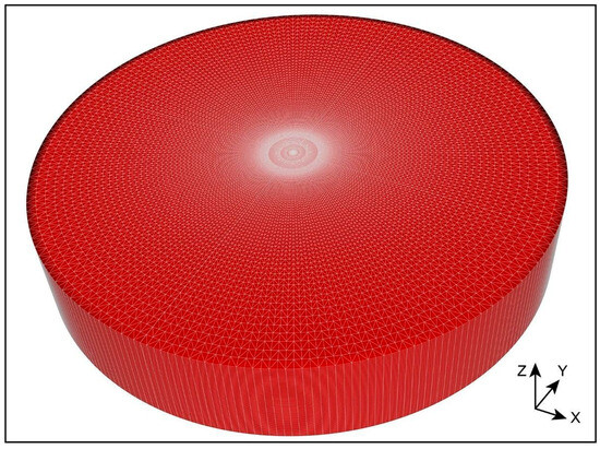
Figure 1.
Domain refinement using triangular and rectangular elements.
The circle representing the cylindrical section of the domain was divided into four equal parts by refining it by 1 m in a cross concentric shape with the axes of the cylinder. The cross-shaped refinement within the domain used 1-m-thick rectangles of varying lengths based on their distance from the center. At the center of the refinement lies a square cell with a lateral length of 1 m, where the central extraction well is located. The lengths of the cells in the cross-shaped refinement created refinement arcs in the four circular sections into which the domain was divided. This domain refinement allowed for a symmetrical control section, which was integrated perfectly into the numerical modeling software, focusing on finite differences or elements. Figure 2 shows an enlarged view of the horizontal plane of the domain, placed at the center of the surface, and illustrates mesh refinement.
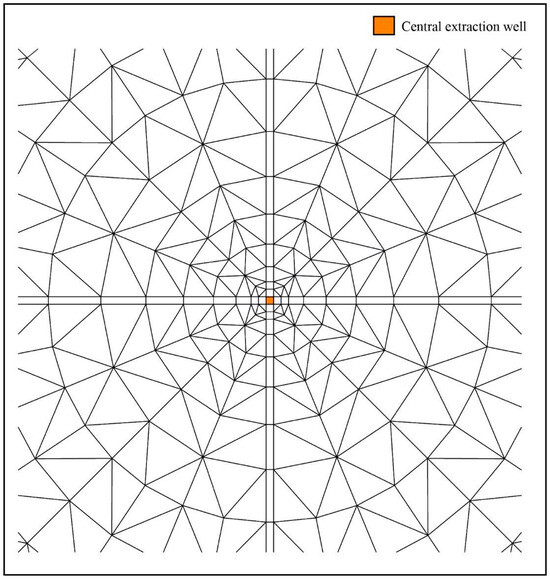
Figure 2.
Visualization of mesh refinement in the central area of the domain surface: enhanced view in a horizontal plane.
The distributed refinement implemented to adequately represent the numerical model dynamics at the domain center did not follow a regular structure. Elements were subdivided based on the arc length they formed as they moved away from the domain center, enabling a moderate element size and number transition. The model mesh, composed of 42,269 elements per numerical layer of a 1 m thickness, varied according to the number of layers corresponding to aquifer thickness, resulting in 1,056,725 elements for 25 m aquifers, 2,113,450 elements for 50 m aquifers, and 3,170,175 elements for 75 m aquifers. Figure 3 illustrates how this subdivision occurred in different sections as it moved away from the domain center.
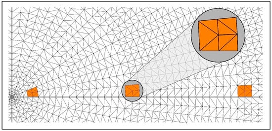
Figure 3.
Gradual subdivision of elements from the center to the edge of the domain, highlighted in orange: enhanced view in a horizontal plane.
2.3. Instruments and Tools
The preprocessing, modeling, and post-processing stages ensured the accuracy and reliability of the simulations and were crucial components of the proposed methodology. Preprocessing involved generating a high-quality mesh, assigning physical properties to the mesh elements, specifying initial and boundary conditions, and selecting appropriate mathematical models and parameters. This stage employed tools such as MODFLOW 6, SEAWAT 4, and FEFLOW 10, along with their respective application programming interfaces (APIs), including FloPy 3.9.3 for MODFLOW 6 and SEAWAT 4 and IFM 10 for FEFLOW 10, to set up and prepare the data for simulation. Modeling utilized hydrogeologic simulation software to solve mathematical equations describing the behavior of a system and required continuous monitoring and parameter adjustments for accuracy. This stage extensively leveraged numerical modeling software, such as MODFLOW 6, SEAWAT 4, and FEFLOW 10, by utilizing their APIs (FloPy and IFM) to facilitate model runs and data integration. Post-processing included visualizing and analyzing the results in detail, generating graphs and maps to interpret the data, and preparing comprehensive reports. Python algorithms enhanced the efficiency and reliability of this process, managed simulations, and achieved the established objectives. The availability of an API in hydrogeologic modeling software streamlines data input and results processing, facilitating method development. The results obtained through the API underwent post-processing using Python algorithms, enabling new data input by adjusting the desired parameters and continuing with an iterative process until the desired outcome was achieved. The APIs and Python algorithms were crucial in the preprocessing, modeling, and post-processing stages to ensure the robustness and efficiency of the method.
Additionally, high-performance computing (HPC) resources were utilized, which is crucial for efficiently validating the method, enabling task parallelization, and enhancing workload performance on a massive scale compared to conventional computers. This tool allowed all scenarios to be addressed through an iterative process until the goal was reached, which would not have been possible on a conventional computer, even with the best hardware characteristics. This study used HPC system resources at the “Centro Nacional de Processamento de Alto Desempenho em São Paulo (CENAPAD-SP).” The system configuration allocated for this project included six parallel nodes, each equipped with 128 cores and 512 GB of memory per node.
2.4. Procedure
Mass displacement in an aquifer due to the density difference between fresh- and saltwater is complex and multidimensional. This displacement is primarily influenced by the interaction between these two water types and the formation of a saltwater wedge at the base of the aquifer. In this transition zone, fresh- and saltwater gradually mix. The boundary conditions and hydrodynamic properties of the aquifer determine the shape and position of the wedge. Furthermore, the saltwater wedge is not static but shifts and spatially varies due to changes in the hydraulic conditions of the aquifer. Mass displacement in an aquifer, concerning the distribution and movement of dissolved components is directly influenced by the dynamics of the saltwater wedge. Variations in the saltwater wedge can significantly alter flow patterns and solute transport within the aquifer. This displacement is complex in four dimensions because solutes can move horizontally and vertically through the aquifer due to density gradients and differences in hydrodynamic parameters, such as hydraulic conductivity, vertical anisotropy, specific yield, and mechanical dispersion. A comprehensive two-step approach is necessary to address mass displacement in aquifers. The first step was to delineate the spatiotemporal variations in the saltwater wedge and their impact on the aquifer within the scenarios proposed for applying the method. The second step was to optimize mass extraction based on the hydraulic conductivity of each scenario. These steps aimed for homogeneous mass displacement throughout the aquifer’s thickness in the shortest possible time, minimizing the saltwater wedge effect at the base of the aquifer.
2.4.1. Spatiotemporal Delimitation of the System
The system design is explained as an evolution of stages, as illustrated in subsequent figures. Figure 4 illustrates mass displacement in a 2-D representation of a vertical section from a 3D numerical model of an aquifer 1800 days after implementing the method. This model features a homogeneous isotropic aquifer with a hydraulic conductivity of 5 m/d, a homogeneous initial salt concentration of 35 kg/m3, and a fully penetrating freshwater injection well with a constant flow rate of 1 L/s. Mass displacement through concentration isolines ranged from 0.5 to 17.5 kg/m3, excluding mechanical dispersion and molecular diffusion effects. The angle between a specific point on a given concentration isoline and the vertical direction (θ) provides additional insight into mass transport dynamics. This angle increases both with concentration and as the isoline approaches the surface. This behavior describes mass displacement that generates a density gradient, where the mass offers more resistance at greater depths and higher concentrations.
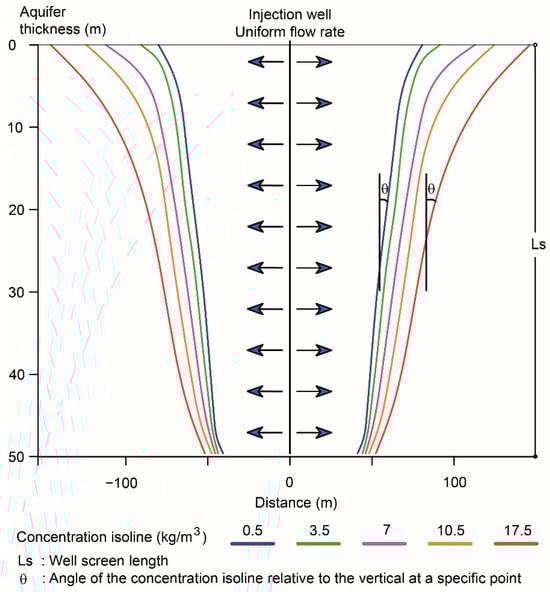
Figure 4.
Density gradient in mass transport within aquifers: simulation example after 1800 days post-method implementation for an aquifer with an initial salt concentration of 35 kg/m3 and a fully penetrating injection well. The arrows represent uniform flow.
An injection well was introduced into the model shown in Figure 4 to enhance mass displacement over time and extract it from the system, thereby boosting the velocity gradient, improving displacement, and preventing concentration increases as the mass moves through the system. Continuing with the same aquifer, Figure 5 shows injection and extraction wells, where the blue arrows indicate the uniform injection of freshwater along the well, while the red arrows indicate uniform extraction. Concentration isolines assess density gradient behavior. The angle between the concentration isolines and the vertical direction (θ) illustrates the resistance to mass displacement near the aquifer bottom compared to the behavior closer to the surface in both extraction and injection wells. However, the angle near the extraction well is notably lower than that close to the injection well due to the combined action of the injection and extraction wells on mass displacement.
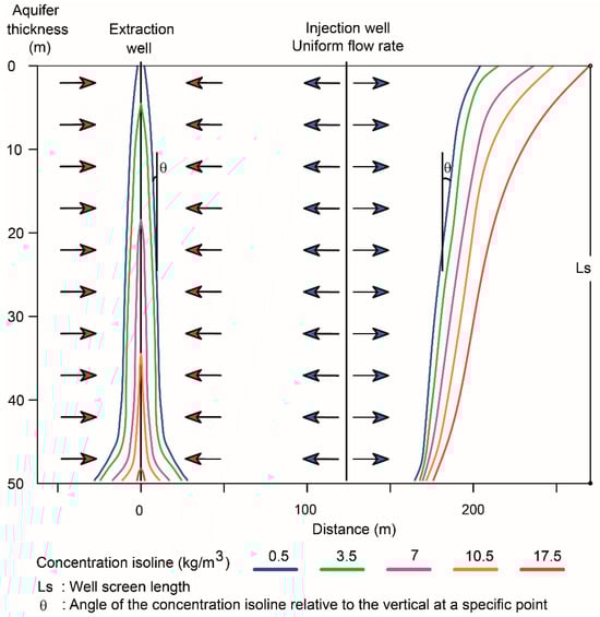
Figure 5.
Density gradient in mass transport within aquifers: simulation example after 1800 days for an aquifer with an initial salt concentration of 35 kg/m3 and fully penetrating injection and extraction wells. The arrows represent uniform flow.
Extending the solution to a 3D format involves inserting four injection wells surrounding an extraction well, as illustrated in Figure 6. The central well is responsible for extracting the combined flow rates injected by the peripheral wells. Injecting fresh water into the peripheral wells induced mass displacement. Subsequently, the mass was attracted toward the extraction central well, facilitating its movement. However, this displacement only covered part of the area between the injection and extraction wells. After 1800 days of simulation, the density gradient observed from the plan view at the model’s top produced a distinct four-leaf clover pattern for the 17.5 kg/m3 concentration isoline (Figure 6a). At greater aquifer depths, the footprint lost its proportion due to the density difference between fresh water and saltwater. Saltwater is denser than fresh water due to dissolved salts, making it heavier per unit volume. This phenomenon caused the footprint to cover more of the surface area and less of the area at the base of the aquifer (Figure 6b).
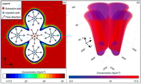
Figure 6.
Mass displacement after 1800 simulation days: (a) in-plan view for the first numerical layer and (b) in 3D view.
Thus, establishing a broader configuration of the extraction and injection wells within a salinized aquifer is possible. The layout of the system can adapt to any direction, considering that each extraction well draws four times the design flow rate (Q), and each injection well introduces a flow rate into the system based on its position within the configuration, following the rule of tributary flow contribution toward the extraction well, as shown in Figure 7. The distribution of the extraction and injection flow rates ensured volumetric compensation of the extracted water against the injected water by adding an equivalent volume to the extracted mass. This method can be implemented in a closed system that extracts water, eliminates contaminants through treatment systems, and continuously injects treated water to avoid polluting effluent generation. The distance between the wells (dw) was calculated in a manner similar to the design flow rate (Q). These variables depend on the hydraulic conductivity, initial salt concentration of the aquifer, and optimal operation time for homogeneous mass displacement throughout the aquifer thickness. Figure 7 shows the well injection and extraction distribution configuration used to analyze the MAR-MASS method.
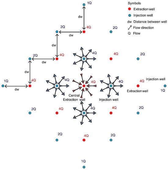
Figure 7.
Distribution of the injection and extraction wells implemented in the MAR-MASS method.
The method implemented in the aquifer emphasizes its high scalability and adaptability, facilitating its application to various target areas regardless of their geometry, as depicted in Figure 8. The distribution of wells and the adjustment of the injection and extraction flow rates according to site requirements ensure customization to maximize mass extraction efficiency. The scalability of the method supports its use in different intervention areas and under diverse hydrogeologic conditions, thereby meeting specific case requirements.
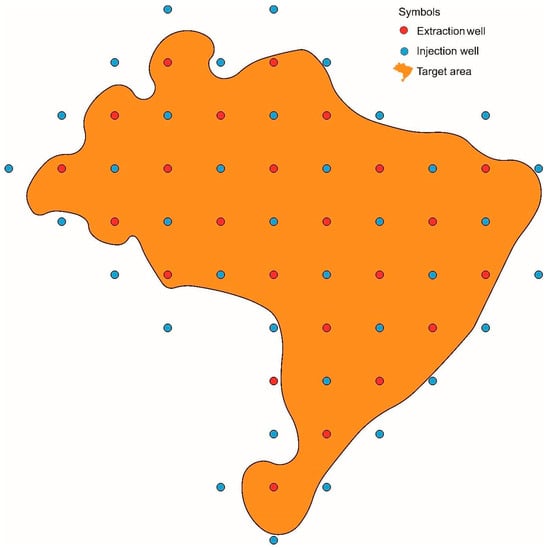
Figure 8.
Example of an injection and extraction well distribution in a target area.
2.4.2. Optimization of Mass Extraction from the System
The optimization process for mass extraction from the system aimed to achieve homogeneous mass displacement from the aquifer base to its surface. Initially, the flow rate of water injected and extracted from an aquifer varied based on hydraulic conductivity and aquifer thickness. Subsequently, three hypothetical flow distribution scenarios in the injection and extraction wells were conceptualized. The third scenario targeted the optimized system conditions, whereas the first scenario represented the traditional injection or extraction flow rate and was uniformly distributed (Q) across the well screen, as shown in Figure 9. Scenario 2 assumed two injection zones: Zone 1 at the top of the well screen and Zone 2 at the base of the aquifer, with a higher uniformly distributed flow rate than that in Zone 1 to counteract the resistance to mass transport at the bottom of the aquifer. Scenario 3 implied gradual injection in zones 1 and 2, following a parabolic pattern that increased with the depth of the well screen, as measured from the top to the base. Figure 9 presents the simulated scenarios for a 50-m-thick aquifer with a hydraulic conductivity of 5 m/d and a flow rate of 5.68 L/s.
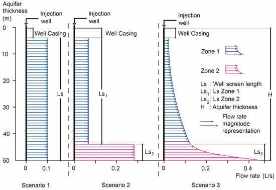
Figure 9.
Injection zones for scenarios 1, 2, and 3 in implementing the MAR-MASS method.
Aquifer hydraulic conductivity and thickness affected the total flow rate injected or extracted by the well (cap . Furthermore, the flow rate distribution per linear meter on the well screen () varied depending on the analyzed scenario and the well screen length (Ls). Equations (1)–(4) represent the flow rates for scenarios 1 and 2.
For Scenario 1:
For Scenario 2, the total flow rate in the well () is the sum of the flow rates assigned to zones 1 () and 2 ():
The flow rate per linear meter for each zone was as follows:
In Scenario 3, the flow rate in each zone gradually increased. This distribution was simplified into two sectors. The first sector (A1) represents a percentage of the flow rate applied uniformly to form a rectangular section on the well screen. The second sector (A2) managed the remaining percentage of the flow rate in the zone, gradually following a parabolic equation. Together, these sectors summed to 100% of the flow rate in the zone. The relationship (p) was used as a control measure or improvement parameter in the methodology framework and adjusted through trial and error. This process involved modifying the parameter to assess its effect, aimed at an optimal operating point. The relationship (p) varied depending on the zone and hydraulic conductivity of the aquifer, thus establishing a connection with the constants of the equation. This relationship, identified here as the distribution coefficient, governed the distribution of the injection or extraction flow rates at the base of the studied zone. Figure 10 presents the details of the variables.
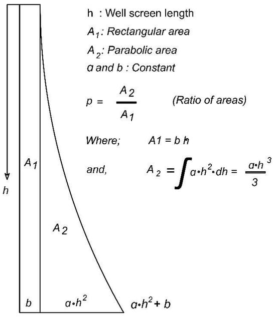
Figure 10.
Geometric and mathematical characterization of the injection zones in Scenario 3 of the MAR-MASS implementation.
Taking from Figure 10:
Simplifying:
Isolating from Equation (6):
Taking from Figure 10:
where represents 100% of the flow assigned to the zone, set to 1, and and represent the proportion in the rectangular and parabolic sections, respectively. Substituting the values of and into Equation (7), the following expression is obtained:
Substituting b from Equation (7), the resulting expression is:
Simplifying:
Multiplying both sides by :
Isolating from Equation (12):
Substituting () in Equation (7):
By considering variables (a) and (b) in Figure 10, an equation was derived to calculate the flow rate within each meter of the well screen () relative to the screen well length and the flow rate of the zone ():
Rewriting Equation (2) for Scenario 3:
For each zone, Equation (15) applies, resulting in the following:
where is the length of the well screen in Zone 1 (m) and is the length of the well screen in Zone 2 (m).
Equations (13) and (14) determine , , , and , leading to the calculation of the flow rate per linear meter () for zones 1 and 2, as described in Equation (17). This results in the following expression:
where ;
where , is in m, is in L/s, and is in L/s/m.
Optimizing mass extraction in Scenario 3 involved increasing the injection and extraction flow rates with depth, divided into two zones (, ). This flow rate is a function of the total flow rate applied per zone (, ), length of each zone (, ), well screen length (h), and distribution coefficients that define the curvature of the parabolic growth of the flow rate (, ). The method evaluated 6960 scenarios, considering each variable and estimating the flow rate for and , based on hydraulic conductivity and aquifer thickness through trial and error, as well as determining the specific well spacing (dw) and zone lengths (, ), with and defined by aquifer thickness. Subsequently, trial and error identified the distribution coefficients (, ) based on hydraulic conductivity. This approach aimed to achieve the best fit for a uniform and efficient mass displacement over time. Figure 11 illustrates the variables considered in the system optimization of the injection wells. For the extraction wells, the values of and were equal in magnitude, but with a negative sign. The design flow rate values required multiplication by a factor that depended on their position in the system, as shown in Figure 7.
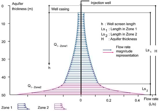
Figure 11.
Injection zones for Scenario 3 in implementing the MAR-MASS method.
3. Results
3.1. Spatiotemporal Optimization and Flow Rate Distribution in Aquifer Systems
Through an iterative process, the method aided in spatially and temporally delimiting the system by varying the injection and extraction flow rates across distances between wells ranging from 50 to 150 m for 6950 scenarios simulated over 3000 days. A distance of 100 m between wells emerged as the optimal choice from both technical and economic perspectives, aligning with the criteria for efficient mass displacement and decreasing density gradients over time. The length of Zone 2 () was determined iteratively, correlating this length with the percentage of aquifer thickness. The analysis considered lengths ranging from 8 to 16% of aquifer thickness, which varied between 25 and 75 m, identifying a size equivalent to 12% to achieve adequate mass displacement at the base of the aquifer. is the result of subtracting the length of Zone 2 () and the well casing from the aquifer thickness. The well casing is a tube without slots that guides the point at which injection and extraction flows begin. The length was adjusted to 6 m through trial and error for aquifers between 25 and 75 m, responding to changes in the water table in the simulated scenarios. Empirical Equations (20) and (21) determine the values of and , presented in Equations (18) and (19), respectively. These equations were derived by trial and error and relate the flow injected and extracted in each zone to the thickness of the aquifer and the hydraulic conductivity governing flow propagation in the system:
where K is the horizontal hydraulic conductivity (m/d) and H is the aquifer thickness (m).
Substituting into Equation (2) yields the total flow applied throughout the well screen:
Empirical Equations (18) and (19) determine the values of and , presented in Equations (23) and (24), respectively. These empirical equations were derived through analysis and trial and error to determine the flow distribution coefficient for each zone. The greater the coefficient value, the greater the magnitude of the flow distribution at the base of the analyzed zone. An appropriate flow distribution allows for uniform mass displacement throughout the aquifer thickness. The distribution coefficients remain constant for different aquifer thicknesses, but are hydraulic conductivity functions:
Figure 12b provides a graphical representation of Equations (23) and (24) for the calculated flow by zone for a 50-m-thick aquifer, along with the distribution coefficient values per zone for any aquifer thickness. Figure 12a for Zone 1 shows that the flow rate increases with a secant slope of 33% between points with hydraulic conductivities of 5–20 m/d. The curve has an inflection point at a conductivity of 30 m/d and ends with a secant slope of 3% between points with conductivities of 40–80 m/d. The secant slope of Zone 2 between points with hydraulic conductivities ranging from 5 to 100 m/d was 9.6%. Regarding the distribution coefficient, the secant slopes between hydraulic conductivities of 5 and 100 m/d for Zones 1 and 2 were 0.3% and 1.8%, respectively.
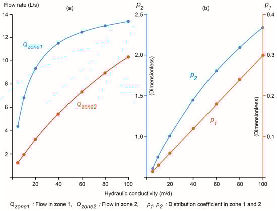
Figure 12.
(a) Flow rate calculated by zone for a 50-m-thick aquifer. (b) Distribution coefficients by zone.
Figure 13 illustrates the flow distribution per linear meter () based on Equations (20) and (21), showing an increase in flow with increased hydraulic conductivity. The analyses considered a 50-m-thick aquifer with a well casing of 6 m. Zones 1 and 2 had lengths of 38 and 6 m, respectively.
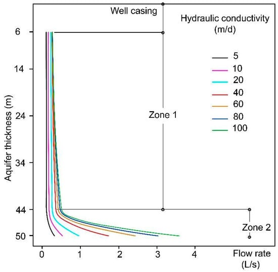
Figure 13.
Flow injection or extraction per linear meter for each hydraulic conductivity of a 50-m-thick aquifer.
3.2. Flow Adjustment and Mass Displacement Outcomes
Mass displacement through the injection and extraction wells implemented in the MAR-MASS method created a boundary effect due to the radius of influence of each well when applied to an area smaller than the remediation zone, as shown in Figure 14. To avoid boundary effects, the well configuration must cover the area of interest; the peripheral freshwater injection wells should form a hydraulic barrier to contain the mass volume to be remediated, as illustrated in Figure 8. Figure 14 shows a plan view of the model with a well spacing (dw) of 100 m. It presents the mass displacement outcome for a 50-m-thick aquifer after an 1800-day simulation, with an initial uniform salt concentration of 35 kg/m3 and a hydraulic conductivity of 5 m/d. The design flow rate calculated using Equation (22) was 5.68 L/s. Using this configuration, the total extraction flow was 36-fold that of the design value, as illustrated in Figure 7, resulting in a total of 204.48 L/s for both extraction and injection.
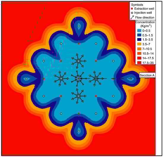
Figure 14.
Mass displacement after 1800 simulation days in the horizontal plane at the model’s top using the MAR-MASS method. Image generated in FEFLOW.
Cross-section A between the central and peripheral injection wells showed a parabolic injection and extraction pattern from the surface of the model to its base (Figure 15). The inclination of the concentration isolines in the peripheral injection well suggests uniform vertical mass displacement along the 0.5 kg/m3 isoline. Figure 15 shows a smoother inclination of the concentration isolines compared to those in Figure 5, prior to applying the equations optimizing mass extraction.
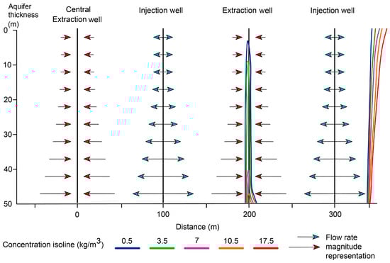
Figure 15.
Cross-section A showing mass displacement through concentration isolines during injection and extraction well operation under the MAR-MASS method.
3.3. Effectiveness of Mass Displacement
Simulations of 6950 scenarios with 3000 days of system operation were used to analyze the different hydraulic parameters and boundary conditions with respect to the time required to reach the target residual concentration. Hydraulic conductivity influences the time required to achieve this goal, with a reduction in the number of days as hydraulic conductivity increases, partly due to the increased extraction and injection flow rates with increasing conductivity. However, this effect diminished at higher initial salt concentrations and was negligible at 35 kg/m3, emphasizing the significant relationship between the initial aquifer salt concentrations and mass displacement, as shown in Figure 16. Analyzing the maximum and minimum times for each concentration revealed a consistent behavioral pattern when plotted on a logarithmic scale. Another aspect to highlight is that for specific yields lower than 0.3, the relationship between different initial concentrations—such as the 5:1 ratio between 3.5 and 17.5 kg/m3—did not correspond proportionally to the number of days required to reach the target concentration between these concentrations. In other words, the time needed to reach the target concentration for 17.5 kg/m3 was not five-fold longer than that for 3.5 kg/m3. Regarding the specific yield, a linear behavior was observed in a logarithmic scale for initial concentrations between 3.5 and 17.5 kg/m3 as the specific yield increased to a value of 0.3. With a specific yield of 0.35, the number of days decreased significantly due to the rapid decrease in stored mass.
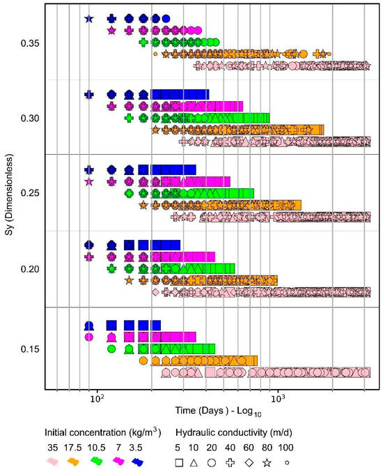
Figure 16.
Time necessary to reach a residual concentration equal to 0.5 kg/m3 versus the specific yield (Sy), according to the initial concentration (color) and hydraulic conductivity (geometric shape).
The vertical anisotropy effect of hydraulic conductivity was not distinguishable when analyzing the time required to reach the target residual salt concentration in the method, as shown in Figure 17a. Molecular diffusion remained irrelevant within this analysis timeframe, leaving only mechanical dispersion as a significant influential variable. Figure 17b illustrates that higher initial salt concentrations highlight the relationship between longitudinal dispersivity, mechanical dispersion, and the time needed to achieve a residual concentration of 0.5 kg/m3. Observing Figure 17a,b on a logarithmic scale shows a linear trend within the initial concentration ranges of 3.5 to 17.5 kg/m3 for each specific yield. As the initial concentration increased, the number of days required to reach the target residual concentration also increased.
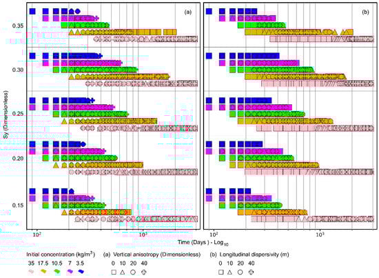
Figure 17.
Time necessary to reach a residual concentration equal to 0.5 kg/m3 versus the specific yield (Sy), according to the initial concentration (color): (a) vertical anisotropy (geometric shape) and (b) longitudinal dispersivity (geometric shape).
Similarly, as shown in Figure 17b, a linear trend indicates an increase in specific yield for initial concentrations of 35 kg/m3 and longitudinal dispersivity values of 0, 10, 20, and 40. Figure 16 and Figure 17 show that for an initial concentration of 3.5 kg/m3, the target concentration was achieved within a maximum of 390 days; for 7 kg/m3, within 600 days; for 10.5 kg/m3, within 840 days; and for 17.5 kg/m3, within 1920 days. At a concentration of 35 kg/m3, 33% of the scenarios did not reach the target concentration within 3000 days, ending with an average residual salt concentration of 0.64 kg/m3. Moreover, of the 6950 scenarios evaluated, 88% achieved the objective in less than 5 years, and 79% within the first 2 years.
3.4. MAR-MASS vs. Conventional Injection Systems
Twenty random scenarios were selected from the 6950 simulations using the same well-spacing configurations to compare the MAR-MASS method with conventional injection systems that use a uniformly distributed flow on the well grid. Figure 18a shows four scenarios for each initial concentration, with blue points representing the scenarios where the MAR-MASS method was implemented. A noticeable contrast was observed in the time required to reach the target residual concentration of 0.5 kg/m3. Compared with scenarios using the conventional injection method (orange points), Scenario 14 showed a 51% reduction in time using the proposed method compared with a conventional injection system, with operation time decreasing from 37 to 19 months. Scenario 10 demonstrated a 10% reduction in operation time from 100 to 10 months. This time could be even shorter because, after 100 days, the residual concentration did not reach the target value, resulting in a concentration of 0.67 kg/m3. The average reduction was 28% in the comparative analysis of 20 scenarios evaluated using the MAR-MASS method and a conventional injection system. Figure 18b displays the maximum pressure in the system for each scenario. The units are in meters of the water column, measured above the maximum hydraulic head value, assigned as the boundary condition of the system. The maximum pressures in the system ranged between 3 and 14 m in the water column when implementing the MAR-MASS method, compared with 21 and 87 m when using the conventional system. This behavior indicates that the MAR-MASS method allows for the better propagation of injected water and consequently facilitates mass transport. The maximum values in Figure 18b correspond to scenarios with hydraulic conductivities of 5 m/d, with values exceeding 85 m in the water column, which could limit the implementation of conventional injection systems. This suggests that implementing the MAR-MASS method covers scenarios where the operation could be feasible and efficient even with low hydraulic conductivities.
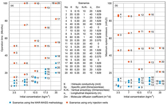
Figure 18.
(a) Time necessary to reach a residual concentration equal to 0.5 kg/m3 versus the initial concentration. (b) Maximum system pressure versus the initial concentration.
4. Discussion
A comparison between the results obtained in this study and the existing literature reveals that the MAR-MASS system constitutes a significant advancement over conventional managed aquifer recharge (MAR) methods, particularly under variable-density flow conditions, such as seawater intrusion or the remediation of dense contaminants. The literature categorizes hydraulic solutions for seawater intrusion control into positive, negative, mixed, and double-pumping barriers, based on the constraints applied to the affected aquifer [1,7,10]. Figure 19a illustrates positive barriers, where freshwater injection forms a hydraulic crest. The effectiveness of this technique relies on placing the injection point at the intersection between the seawater intrusion interface (SWI) and the aquifer bottom [11,12]. However, performance remains constrained by the temporal variability of the SWI [13,14]. Effective repulsion of saline water occurs only when water is injected precisely at the critical junction of freshwater, saltwater, and the aquifer base [11]. Figure 19b shows negative barriers, which rely on water extraction to create low-pressure zones, but typically remove more freshwater than saltwater and entail high energy consumption [15]. Figure 19c,d present mixed and double-pumping barriers, which enhance control over intrusion; however, their efficiency strongly depends on system design, aquifer geometry, and the relative position of the wells [7,16,17].
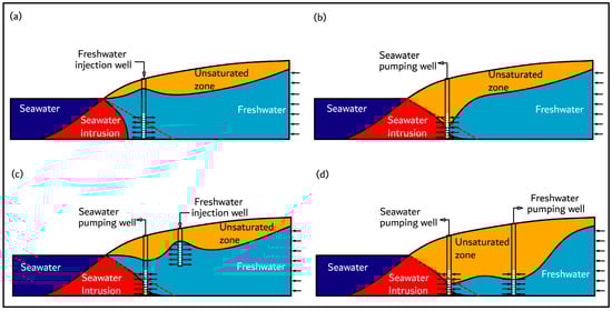
Figure 19.
Hydraulic barriers, adapted from [7]. The red dashed lines represent saline intrusion prior to the implementation of the hydraulic barriers. (a) Positive hydraulic barrier. (b) Negative hydraulic barrier. (c) Mixed hydraulic barrier. (d) Double pumping barriers.
MAR-MASS provides a modular and adaptable solution that enhances the vertical distribution of flow, overcoming key limitations observed in traditional approaches. A major challenge in injection–extraction systems involves achieving homogeneous displacement of the saline or contaminant mass throughout the full thickness of the aquifer [1,7], particularly in media with high anisotropy or low hydraulic conductivity, where density gradients tend to develop and reduce system efficiency [18,19]. Numerical results indicate that, compared to conventional methods, MAR-MASS reduces recovery times by 90% to 50% across most simulated scenarios, aligning with efficiency improvement trends associated with the optimization of injection/extraction well pairs in coastal aquifers [16], while also extending applicability to a broader range of geological conditions and contamination types [5]. This enhanced hydraulic efficiency not only lowers operational and energy requirements but also directly contributes to carbon emission reduction by shortening the time and energy needed to achieve remediation goals [20,21].
MAR-MASS emerges as a scalable and adaptable alternative for sustainable groundwater management. Its modular design, featuring vertically differentiated flow distribution, enhances hydraulic front control, reduces resistance in deeper zones, attenuates density gradients, and promotes the advancement of fresh water—even in heterogeneous or low-permeability media, where conventional approaches prove less effective. Comparative analysis of maximum pressures indicates operational feasibility in conditions where traditional methods tend to generate excessive or unviable pressures, making MAR-MASS particularly suitable for low-conductivity aquifers.
This capacity contrasts with the limitations of widely applied technologies such as pump-and-treat systems, which, despite their extensive use, often underperform in heterogeneous settings. Contaminant stagnation, prolonged remediation times, and low recovery efficiency are frequently reported under such conditions [22,23]. Field-scale dispersion and aquifer heterogeneity further constrain effectiveness [24].
Despite the potential demonstrated in numerical simulations, large-scale implementation of MAR-MASS demands rigorous experimental validation and careful assessment of site-specific hydrogeological and operational conditions. Such caution remains essential to avoid uncritical adoption of methods whose simulated performance may be overestimated when applied in real-world scenarios.
5. Conclusions
The MAR-MASS method demonstrated its effectiveness in extracting mass from aquifers of different densities, substantially contributing to sustainable water resource management by presenting significant advantages over conventional injection systems. The proper distribution of injection and extraction wells and depth-varying flow promote uniform mass displacement throughout the aquifer, reducing density gradients and increasing extraction efficiency over time. Simulating multiple scenarios with different hydrogeologic variables, such as vertical anisotropy, specific yield, mechanical dispersion, and molecular diffusion, provides valuable information for optimizing mass extraction processes. MAR-MASS provides solutions to SWI or issues involving flows of different densities within the continent due to masses originating from the dissolution of natural or anthropogenic constituents, with mass concentrations ranging from 3.5 to 35 kg/m3.
The hydraulic conductivity and specific yield of an aquifer are pivotal parameters that affect the duration required to achieve desired residual concentrations, with a decrease in the timeframe as hydraulic conductivity increases and specific yield diminishes. These findings further suggest that the time required to reach target residual concentrations varies depending on the initial concentration of the aquifer, with mechanical dispersion exerting a significant impact on this process. The proposed MAR-MASS injection and extraction system effectively combats resistance and opposition to mass movement at greater aquifer depths, enhancing the spread of injected water and facilitating mass transport. Simulations demonstrated exceptional operational efficiency, enabling the attainment of the target residual concentration in the intervened area within 50 to 10% of the time required by a conventional injection system with equivalent water flow resources.
The MAR-MASS system has proven to be flexible and adaptable to various hydrogeologic conditions across a range of conductivities and characteristic parameters in aquifers with thicknesses between 25 and 75 m and comprising unconsolidated materials, such as medium and coarse sand and a mixture of sand and gravel. The system’s spatiotemporal approach enabled the scalability of MAR-MASS, ensuring its adaptability to different target areas and hydrogeologic conditions, thus guaranteeing its practical application in various contexts. Implementing a cyclic extraction, treatment, and injection system prevents polluting effluent generation. The findings of this study support the efficacy and relevance of MAR-MASS in optimizing mass extraction in aquifers, emphasizing its potential to enhance groundwater management and promote sustainable aquifer recharge practices.
Integrating programming tools, such as Python, with advanced technological strategies, such as parallelization techniques and HPC, significantly improved the development and validation of MAR-MASS. This study emphasizes the usefulness of these tools for performing intricate calculations, analyzing extensive datasets, and managing databases within hydrogeological models. The utilization of APIs, such as IFM in the FEFLOW numerical modeling software and Flopy in MODFLOW, further highlights the sophistication and accuracy of the method, enabling detailed simulations and optimizations. Combining these technologies is crucial for achieving precise and efficient results that cannot be achieved using traditional methods, highlighting the vital role of state-of-the-art technologies in advanced hydrogeologic research.
Although the MAR-MASS method has shown significant potential within numerical modeling analysis, future studies should perform field validation to confirm the method’s applicability in diverse environments. Additionally, the application of the MAR-MASS method in the remediation of contaminated areas can be explored, with the extraction of masses of different contaminants.
MAR-MASS establishes a robust foundation for future research and practical applications in hydrogeology and water resource management, thereby benefiting the scientific community and society.
Author Contributions
M.A.G.T.: conceptualization; methodology; validation; formal analysis; investigation; writing—original draft preparation. A.S. and L.C.F.: writing—review and editing; supervision. All authors have read and agreed to the published version of the manuscript.
Funding
This research received no external funding.
Data Availability Statement
The data supporting the findings of this study are available from the corresponding author upon reasonable request. Due to the complexity, size, and technical specificity of the datasets, including source code and procedures developed over several years—public sharing may not be efficient or appropriate. Controlled access ensures proper use, preserves intellectual property, and mitigates the risk of unauthorized reuse or misinterpretation. All relevant data can be provided to qualified researchers or reviewers upon request and with appropriate context.
Acknowledgments
We gratefully acknowledge the financial support from the Coordenação de Aperfeiçoamento de Pessoal de Nível Superior (CAPES) through the PEC-PG scholarship (Process No. 88881.283987/2018-01), which was essential for this research. We also thank the Centro Nacional de Processamento de Alto Desempenho em São Paulo (CENAPAD-SP) for providing the computational resources used in the development of the numerical models and simulations.
Conflicts of Interest
The manuscript and the data presented herein have not been previously published and are not under consideration for publication elsewhere. All authors declare no conflicts of interest related to this research. All authors have read and agreed to the submitted version of the manuscript for consideration for publication in the Journal.
References
- Maliva, R.G. Anthropogenic Aquifer Recharge: Wsp Methods in Water Resources Evaluation Series No. 5; Springer International Publishing: Berlin/Heidelberg, Germany, 2020; Available online: http://link.springer.com/10.1007/978-3-030-11084-0 (accessed on 10 October 2024).
- Sharifinia, M.; Ramezanpour, Z.; Imanpour Namin, J.; Mahmoudifard, A.; Rahmani, T. Water quality assessment of the Zarivar Lake using physico-chemical parameters and NSF-WQI indicator, Kurdistan Province-Iran. Int. J. Adv. Biol. Biomed. Res. 2013, 1, 302–312. [Google Scholar]
- Sousa, C.; Roseta-Palma, C.; Martins, L.F. Economic growth and transport: On the road to sustainability. Nat. Resour. Forum 2015, 39, 3–14. [Google Scholar] [CrossRef]
- Alhalbaasi, J.; Alhadiathy, A.; Al-Paruany, K. Investigation the origins of groundwater salinity in Baghdad city by using environmental isotopes and hydrochemical techniques. Iraqi Geol. J. 2022, 55, 209–220. [Google Scholar] [CrossRef]
- Rachid, G.; Alameddine, I.; El-Fadel, M. Management of saltwater intrusion in data-scarce coastal aquifers: Impacts of seasonality, water deficit, and land use. Water Resour. Manag. 2021, 35, 5139–5153. [Google Scholar] [CrossRef]
- Fetter, C.W.; Kreamer, D. Chapter 10: Water Quality and Groundwater Contamination. In Applied Hydrogeology: Fifth Edition; Waveland Press: Long Grove, IL, USA, 2021; pp. 393–452. Available online: https://books.google.com.br/books?id=1lFPEAAAQBAJ (accessed on 10 October 2024).
- Pool, M.; Carrera, J. Dynamics of negative hydraulic barriers to prevent seawater intrusion. Hydrogeol. J. 2010, 18, 95–105. [Google Scholar] [CrossRef]
- Johnson, A.I. Specific Yield: Compilation of Specific Yields for Various Materials (Número 1662); US Government Printing Office: Washington, DC, USA, 1967.
- Kruseman, G.P.; de Ridder, N.A.; Verweij, J.M. Analysis and Evaluation of Pumping Test Data; ILRI: Addis Ababa, Ethiopia, 1994; Available online: https://books.google.com.br/books?id=7vNstgAACAAJ (accessed on 10 October 2024).
- Todd, D.K. Salt-Water Intrusion and Its Control. J. Am. Water Work. Assoc. 1974, 66, 180–187. [Google Scholar] [CrossRef]
- Luyun, R.; Kazuro, M.; Kei, N. Effects of Recharge Wells and Flow Barriers on Seawater Intrusion. Ground Water 2011, 49, 239–249. [Google Scholar] [CrossRef]
- Botero-Acosta, A.; Donado, L.D. Laboratory Scale Simulation of Hydraulic Barriers to Seawater Intrusion in Confined Coastal Aquifers Considering the Effects of Stratification. Procedia Environ. Sci. 2015, 25, 36–43. [Google Scholar] [CrossRef]
- Chun, J.A.; Lim, C.; Kim, D.; Kim, J.S. Assessing Impacts of Climate Change and Sea-Level Rise on Seawater Intrusion in a Coastal Aquifer. Water 2018, 10, 357. [Google Scholar] [CrossRef]
- Yu, X.; Wu, L.; Yu, X.; Xin, P. Tidal Fluctuations Relieve Coastal Seawater Intrusion Caused by Groundwater Pumping. Mar. Pollut. Bull. 2022, 184, 114231. [Google Scholar] [CrossRef]
- Sriapai, T.; Walsri, C.; Phueakphum, D.; Fuenkajorn, K. Physical model simulations of seawater intrusion in unconfined aquifer. Songklanakarin J. Sci. Technol. 2012, 34, 679–687. [Google Scholar]
- Lu, C.; Werner, A.D.; Simmons, C.T.; Robinson, N.I.; Luo, J. Maximizing Net Extraction Using an Injection-Extraction Well Pair in a Coastal Aquifer. Groundwater 2013, 51, 219–228. [Google Scholar] [CrossRef]
- Abd-Elhamid, H.F.; Javadi, A.A. A Cost-Effective Method to Control Seawater Intrusion in Coastal Aquifers. Water Resour. Manag. 2011, 25, 2755–2780. [Google Scholar] [CrossRef]
- Abarca, E.; Carrera, J.; Sánchez-Vila, X.; Dentz, M. Anisotropic dispersive Henry problem. Adv. Water Resour. 2007, 30, 913–926. [Google Scholar] [CrossRef]
- Yu, X.; Michael, H.A. Mechanisms, configuration typology, and vulnerability of pumping-induced seawater intrusion in heterogeneous aquifers. Adv. Water Resour. 2019, 128, 117–128. [Google Scholar] [CrossRef]
- Henao Casas, J.D.; Fernández Escalante, E.; Calero Gil, R.; Ayuga, F. Managed Aquifer Recharge as a Low-Regret Measure for Climate Change Adaptation: Insights from Los Arenales, Spain. Water 2022, 14, 3703. [Google Scholar] [CrossRef]
- Ross, A. Benefits and Costs of Managed Aquifer Recharge: Further Evidence. Water 2022, 14, 3257. [Google Scholar] [CrossRef]
- Song, Z.; Wang, Y.; Wang, J.; Huan, H.; Li, H. Design of Pump-and-Treat Strategies for Contaminated Groundwater Remediation Using Numerical Modeling: A Case Study. Water 2024, 16, 3665. [Google Scholar] [CrossRef]
- Guo, Z.; Brusseau, M.L.; Fogg, G.E. Determining the Long-Term Operational Performance of Pump and Treat and the Possibility of Closure for a Large TCE Plume. J. Hazard. Mater. 2019, 365, 796–803. [Google Scholar] [CrossRef]
- Gelhar, L.W.; Welty, C.; Rehfeldt, K.R. A critical review of data on field-scale dispersion in aquifers. Water Resour. Res. 1992, 28, 1955–1974. [Google Scholar] [CrossRef]
Disclaimer/Publisher’s Note: The statements, opinions and data contained in all publications are solely those of the individual author(s) and contributor(s) and not of MDPI and/or the editor(s). MDPI and/or the editor(s) disclaim responsibility for any injury to people or property resulting from any ideas, methods, instructions or products referred to in the content. |
© 2025 by the authors. Licensee MDPI, Basel, Switzerland. This article is an open access article distributed under the terms and conditions of the Creative Commons Attribution (CC BY) license (https://creativecommons.org/licenses/by/4.0/).