2D CFD Modeling of Rapid Water Filling with Air Valves Using OpenFOAM

Abstract

The rapid filling process in pressurized pipelines has been extensively studied using mathematical models. On the other hand, the application of computational fluid dynamics models has emerged during the last decade, which considers the development of CFD models that simulate the filling of pipes with entrapped air, and without air expulsion. Currently, studies of CFD models representing rapid filling in pipes with entrapped air and with air expulsion are scarce in the literature. In this paper, a two-dimensional model is developed using OpenFOAM software to evaluate the hydraulic performance of the rapid filling process in a hydraulic installation with an air valve, considering different air pocket sizes and pressure impulsion by means of a hydro-pneumatic tank. The two-dimensional CFD model captures the pressure evolution in the air pocket very well with respect to experimental and mathematical model results, and produces improved results with respect to existing mathematical models.

1. Introduction

Filling and emptying processes in pressurized pipelines are common practices when it comes to carrying out maintenance and repair work on networks by technical personnel [1]. When such activities are carried out, an interaction between two fluids occurs inside the pipelines: air and water. Air entrapped in pipes has been a problem that causes (i) increases in the absolute pressure of the system, (ii) vibrations in the system due to abrupt changes in velocity, and (iii) corrosion due to temperature changes [2]. When it comes to filling processes, the water that enters the system by means of a hydraulic impulsion begins to occupy the space occupied by the air, generating the compression of the air pocket, which causes overpressures [3,4,5,6].

For the study of the hydraulic phenomena resulting from filling processes in pipes with entrapped air, research has been carried out through the development of mathematical models based on a piston flow analysis that simulate the water–air interface, analyzing the liquid phase, such as rigid column models [7,8,9,10] and elastic column models [6,11,12,13]. The authors of [14,15] have proposed a mathematical model for the analysis of hydraulic transients that occur during rapid filling. They have obtained good approximation of the maximum pressures reached within a cast-iron pipeline of 1020 m length and DN400 of nominal diameter. The authors of [16] presented a mathematical model to simulate rapid filling processes and to simulate the hydraulic and thermodynamic variables in an experimental facility of 7 m length and 63 mm DN of nominal diameter, where they determined that mathematical model is suitable for the reproduction of the first oscillation in the pressure evolution and extreme values of pressure during the filling process. The authors of [17] displayed the limitations of one-dimensional models under certain scenarios that can be overcome using of two- and three-dimensional models.

Computational Fluid Dynamics (CFD) models in 2D and 3D can, in turn, be used to analyze scenarios where air pockets interact with water columns in pressurized pipes, allowing precise determination of space-time behaviour of the transient event generated during the rapid filling process. Currently, different authors have proposed CFD models to simulate rapid filling in pipelines with air entrapped. The authors of [5] assessed the performance of a 3D CFD model simulating the filling process without an air valve and with an entrapped air pocket. They obtained good agreement of the evolution of the pressure. The authors of [18] compared the results of mathematical (1D) and experimental models with 2D numerical models of overpressure patterns of entrapped air pockets in pipes, in which different mesh structures are applied to compare computational convergence criteria, and computational times. The authors of [19] simulated the transient phenomenon generated during the rapid filling process with entrapped air using 2D and 3D CFD models. The authors of [20] created a VOF model applying a numerical solution for the analysis of overpressure generated in entrapped air in pipes during rapid filling processes. Rapid filling in pipelines using the CFD models has been extensively explored through the application of 2D and 3D CFD models; however, CFD models for the simulation of rapid filling of pipelines with entrapped air, and considering air discharge through air valves, has received scarce attention in the research area. In the present research, a two-dimensional CFD model is proposed using the software Open-Source OpenFOAM, where obtained results are compared with experimental pressure measurements done with a pressure transducer located in a high point of an irregular pipeline system and validating the results. The inlet pressure is regulated by a hydro-pneumatic tank, and the air release is regulated by an air valve S050 (A.R.I. manufacturer) with an internal diameter of 3.175 mm. This paper presents the results of 2D CFD simulations of the rapid filling process of water with an air valve. The two-dimensional CFD model accurately represents the pressure behaviour in the air pocket, and it is able to do so due to its ability to capture the deformation of the air pocket in space-time during the compression and expansion stages.

2. Materials and Methods

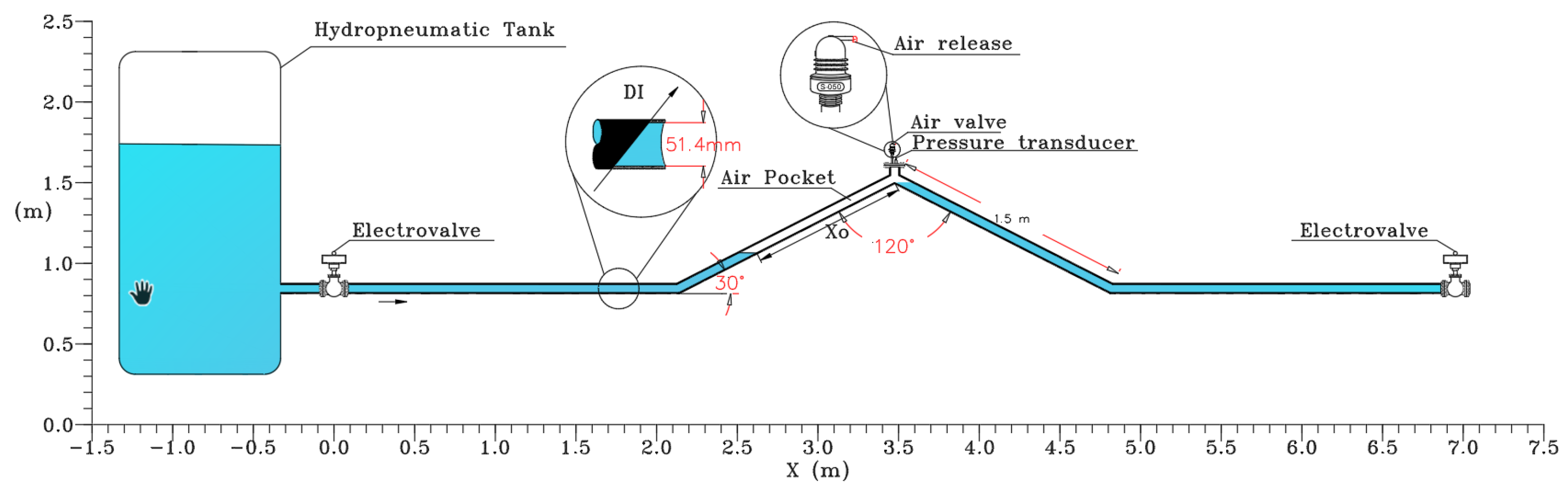
2.1. Experimental Facility

The pressures in the air pockets simulated by the CFD model are compared with the Experimental Test pressures collected in [16] in the hydraulic lab located at the University of Lisbon, Portugal. The hydraulic installation is made up of an irregular polyvinyl chloride (PVC) pipe with a nominal diameter of 63 mm, which has a total length of 7.30 m, with horizontal reaches of 2.05 m, and inclined reaches at an angle of 30° with lengths of 1.50 m. Tests were done using a hydro-pneumatic tank of 1 m³ to produce the inlet pressure. The pipe system is made up of an air valve S050 (manufacturer A.R.I.) with a inner diameter of 3175 mm and an outflow discharge coefficient of 0.32, which was theoretically calibrated by means an air valve characterization curve (see Figure 1). A pressure transducer was located next to the air valve at the highest point of the pipe system to measure the pressure patterns. The regulation of the system is managed by a PVC-U +GF+ electro-pneumatic ball valve type 230 (Georg Fischer Piping Systems Ltd., Schaffhausen, Switzerland). For all simulations, for the experimental facility, only the electro-pneumatic ball valve located in the section connected to the hydropneumatic tank is activated, for which a full opening is given with an opening time of 0.2 s. Figure 2 shows the experimental components.

Figure 1. Characteristic outflow discharge coefficient in air valve S050.

Figure 2. Conceptual scheme of the experimental facility.

For the experimental facility, the hydropneumatic tank is activated and the electro-pneumatic ball valve is opened to allow water to enter from the tank; as the pipe fills, the pressure transducer measures the pressure patterns generated in the air pocket located in the upper part of the irregular pipe, which has a frequency of data collection of 0.0062 Hz. The water hammer effect was considered for both water and air (water hammer with entrapped air). During the measurements, the compression effect of the air pocket due to the displacement of the water column that is pumped by the hydro-pneumatic tank is considered. The authors of [16] conducted six experiments with two initial air pocket lengths ($X_0$ of 0.96 and 1.36 m) and gauge pressures guaranteed by the hydropneumatic tank ($P_i$ = 2.03, 5.09, and 7.64 mwc). See Table 1 for more details.

Table 1. Test characteristics.

Experimental Test	${\mathit{P}}_{\mathit{i}}$ (mwc)	${\mathit{X}}_0$ (m)
1	2.03	0.96
2	2.03	1.36
3	5.09	0.96
4	5.09	1.36
5	7.64	0.96
6	7.64	1.36

2.2. 1D Mathematical Model

The reference mathematical model was proposed by the authors of [16], which analyzes the rapid filling process of an irregular pipe, considering the effect of air discharge by means of an air valve. This model considers some assumptions: (i) the filling of the water column is modeled using a rigid column model, (ii) the air–water interface is considered perpendicular to the main direction of a single pipe, (iii) the friction factor is constant over the transient event;, and (iv) a polytropic model describes the air phase. The initial and boundary conditions consider an initial time t = 0, where the water and air velocity, displaced water column length, and change in air pocket pressure is zero. The air density at the start is equal to $rh{o}_a$ = 1.205 kg/m³. The fundamental equations of the mathematical model are Equations (1) through (5).

$$\frac{d{v}_w}{dt}=\frac{p_0-p_1}{{\rho }_w{L}_w}+g\frac{\delta z_1}{L_w}-f\frac{v_w\left|v_w\right|}{2D_p}-\frac{R_{bv}g{A_p}^2{v}_w\left|v_w\right|}{L_w}$$

(1)

$$\frac{d{L}_w}{dt}=v_w$$

(2)

$$\frac{d{p}_1}{dt}=k_p\frac{p_1}{V_a}\left(\frac{d{V}_a}{dt}-\frac{1}{{\rho }_a}\frac{d{m}_a}{dt}\right)$$

(3)

$$\frac{d{m}_a}{dt}=-{\rho }_a{v}_a{A}_v$$

(4)

$$v_a=C_d{p}_1\sqrt{\frac{7}{RT}\left[{\left(\frac{p_{atm}}{p_1}\right)}^{1.4286}-{\left(\frac{p_{atm}}{p_1}\right)}^{1.714}\right]}$$

(5)

where $v_w$ and $v_a$ are the velocity of water and air, respectively; $L_w$ = water column length; $p_0$, $p_1$, and $p_{atm}$ are the inlet pressure, absolute pressure, and atmospheric pressure condition of the air pocket, respectively; $D_p$ = pipe inner diameter; f = friction factor; $R_{bv}$ = valve friction coefficient; g = gravitational acceleration; $A_p$ and $A_v$ correspond to cross section of pipe and air valve, respectively; $k_p$ = polytropic coefficient; $V_a$ and $m_a$ are the volume and mass of air pocket, respectively; ${\rho }_w$ and ${\rho }_a$ are the water and air density; $c_d$ = discharge coefficient of air valve; R = universal gas constant; and T = temperature.

3. 2D CFD Model

2D CFD models are characterized by their simplifications of experimental models, which have an advantage due to their usefulness in the verification of the interaction between fluids and the computational time savings generated.

3.1. Governing Equations

For the analysis of the transient event, the CFD numerical modeling has been carried out with two-phase flow and compressible (air) using the finite volume method along with the volume of fluid (VOF) method. This model applies the following equations.

3.1.1. Continuity Equation

The term $\frac{\partial \rho }{\partial t}$ in Equation (6) indicates the variation of control volume density over time. Second, $\nabla \left(\rho \mathbf{u}\right)$ represents inflow and outflow over control volume surface. The given equation is defined as

$$\frac{\partial \rho }{\partial t}+\nabla ·\left(\rho \mathbf{u}\right)=0$$

(6)

where $\rho$ is the density of water or air in the studied cell, t represents time, and $\mathbf{u}$ is the velocity vector of the fluid.

3.1.2. Conservation of Momentum Equation

The conservation of momentum equation is based on Newton’s second law, which considers the forces acting on fluids, such as those generated by gravitational, shear, and pressure stresses.

$$\rho \left(\frac{\partial \mathbf{u}}{\partial t}+\mathbf{u}·\nabla \mathbf{u}\right)=-\nabla p+\mu {\nabla }^2\mathbf{u}+\frac{1}{3}\mu \nabla (\nabla ·\mathbf{u})+\rho \mathbf{g}$$

(7)

where p is the pressure, $\mu$ is the dynamic viscosity, and $\mathbf{g}$ is the gravitational deceleration vector.

3.1.3. Volume Fraction Transport Equation

Reynolds transport equation is applied to a discontinuous air–water volume fraction ($\gamma$), which takes values between 0 and 1 in each domain cell (VOF method). If $\gamma$ = 0, this indicates that there is only air presence; if $\gamma$ = 1, the domain is completely occupied by water; mean values indicate the presence of mixed water and air. This is estimated by the following equation:

$$\frac{\partial \gamma }{\partial t}+\nabla ·\left(\gamma \mathbf{u}\right)+\nabla ·\left(\gamma \left(1-\gamma \right)U_r\right)=\frac{-\gamma }{{\rho }_a}\left(\frac{\partial {\rho }_a}{\partial t}+\mathbf{u}·\nabla {\rho }_a\right)$$

(8)

where $U_r$ is a supplementary velocity field for the compression of the interface introduced by the Multidimensional Universal Limiter for Explicit Solution (MULES) solver for $\gamma$. The density and viscosity according to the fraction are, thus, the following:

$$\rho =\gamma {\rho }_w+\left(1-\gamma \right){\rho }_a$$

(9)

$$\mu =\gamma {\mu }_w+\left(1-\gamma \right){\mu }_a$$

(10)

where ${\rho }_w$ is the density of the water; ${\rho }_a$ is the density of the air; and ${\mu }_a$ and ${\mu }_w$ are the viscosity of air and water, respectively. The density and viscosity of the water and the viscosity of the air remain constant over the transient event. The air density is determined using the ideal gas law, therefore

$${\rho }_a=\frac{Mp}{RT}$$

(11)

3.1.4. Energy Conservation Equations

The energy conservation equation is expressed according to temperature as

$$\frac{\partial }{\partial t}\left(\rho T\right)+\left(\rho T·\nabla \mathbf{u}\right)=\nabla ·\left(a_{\mathrm{eff}}\nabla T\right)-\left(\frac{\gamma }{C_{v_w}}+\frac{1-\gamma }{C_{v_a}}\right)\left(\nabla ·\left(p\mathbf{u}\right)+\frac{\partial \left(\rho K\right)}{\partial t}+\nabla ·\left(\rho K\mathbf{u}\right)\right)$$

(12)

where K equals 0.5 ${\mathbf{u}}^2$ (kinetic energy), $C_{v_w}$ corresponds to specific heat in a constant volume of the water, and $C_{v_a}$ is the specific heat in a constant volume of air. $a_{\mathrm{eff}}$ is defined as

$$a_{\mathrm{eff}}=\frac{\gamma k_{t_w}}{C_{v_w}}+\frac{\left(1-\gamma \right)k_{t_a}}{C_{v_a}}+\frac{{\mu }_{tur}}{{\sigma }_{tur}}$$

(13)

where $k_{t_a}$ and $k_{t_w}$ indicate the thermal conductivity of air and water, respectively; ${\sigma }_{tur}$ is the turbulent Prandtl number (0.9); and ${\mu }_{tur}$ is the turbulent kinematic viscosity determined by Menter k-ω SST model.

3.2. Numerical Solution with OpenFOAM

Open-Source Operation and Manipulation (OpenFOAM) is a free, open-source CFD software package that employs libraries for numerical solution of ordinary and high order, linear and nonlinear, partial differential equations ([21]). The mesh was created using the BlockMesh utility, and the ParaView application was employed for pre- and postprocessing.

3.2.1. CFD Model Configuration

A 2D model has been set up using OpenFOAM for the simulation of rapid filling processes with air valve. The following aspects were considered.

• The $X$-axis corresponds to the longitudinal direction which matches the main direction of the flow. The computation domain extends from $X_{min}$ (−0.20 m) up to $X_{max}$ (3.60 m).
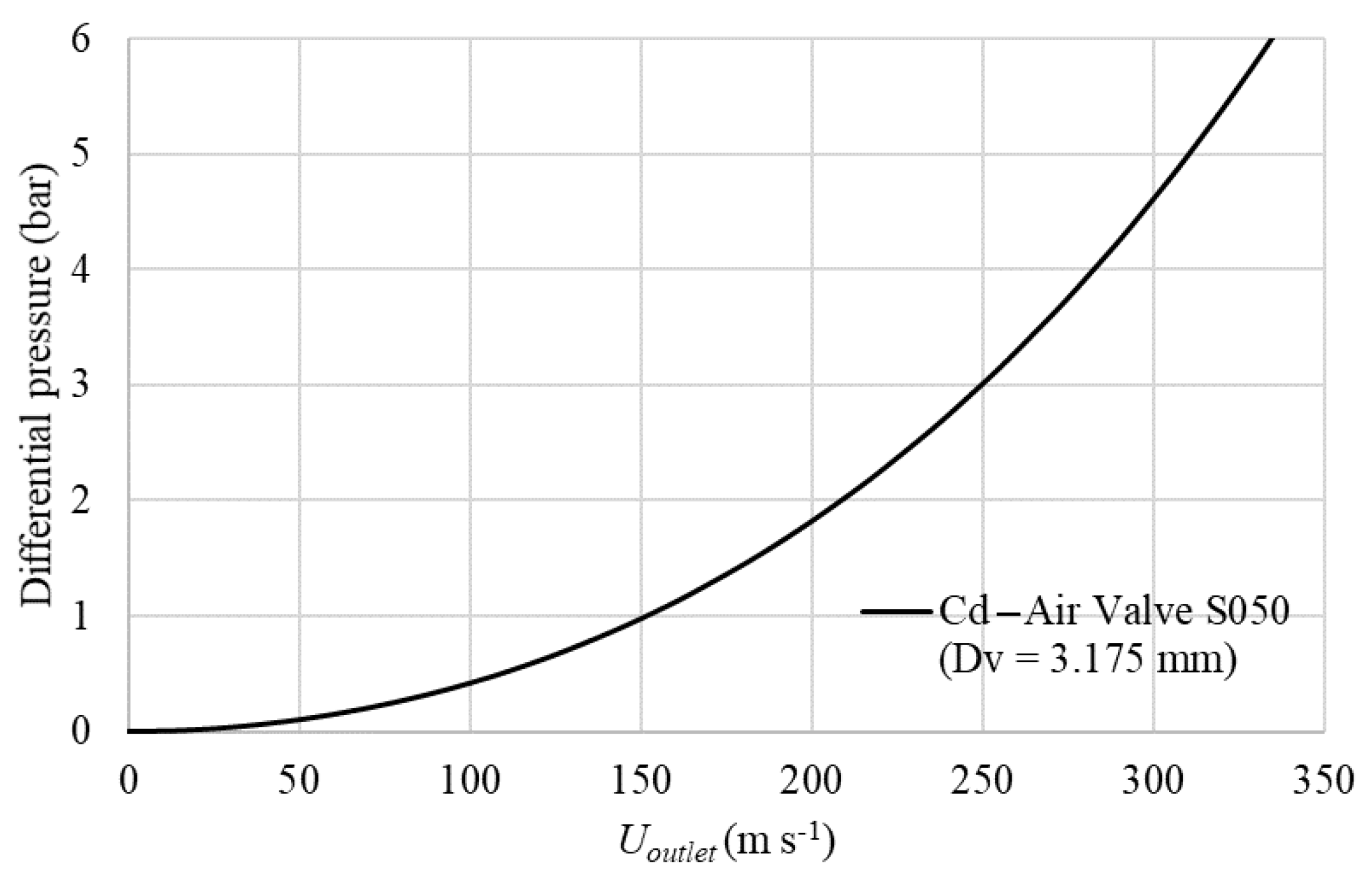
• On the $Y$-axis the installation diameter was considered, setting it to the 3.175 mm air valve diameter (S050 Model). This setup was created for a domain between $Y_{min}$ (−0.0257) and $Y_{max}$ (0.83 m).
• The coordinate system center of the domain was placed in the center of the electro-pneumatic valve.
• The model consists of 25 blocks composed by 31,532 cells, of which 31,404 are hexagonal and 128 are multifaceted polygonal cells.

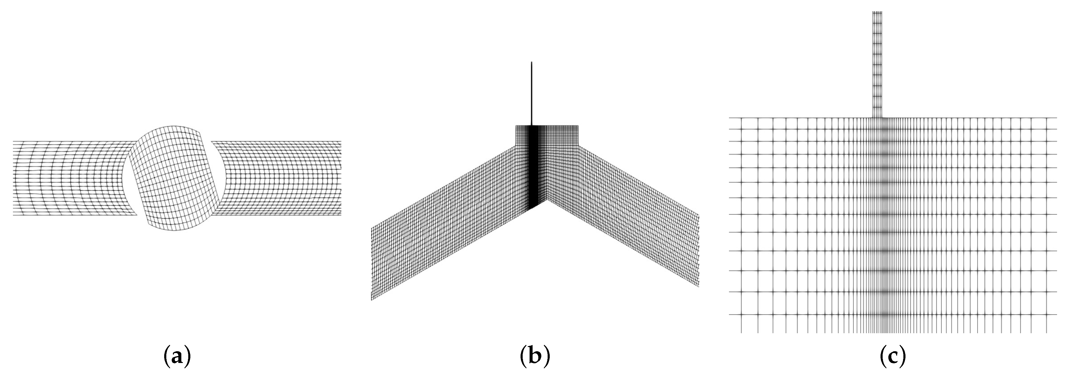
3.2.2. Geometry and Mesh

The system is split in two zones:

• A dynamic mesh representing the opening motion of the electro-pneumatic valve by a solid body motion function (Figure 3a,b). The opening phase of the electro-pneumatic valve occurs from time t = 0.0 s to a time t = 0.2 s. The valve rotation was represented by a tabulation of rotation versus time data.
  

  Figure 3. Geometry and mesh of the CFD model. (a) Opening movement of the electro-pneumatic. (b) Mesh structure in the placement of the S050 air valve. (c) Refinement towards the inlet port of the S050 air valve.
• A set of fixed blocks that represent the pipeline segments of the experimental set-up where the S050 valve was placed (Figure 3b,c). As suggested by [22], the best cell layout for 3D models was chosen, adapted to a 2D scenario.

The geometry and mesh are presented in Figure 3, as they were generated by OpenFOAM’s BlockMesh utility, including the shape and refinement of the mesh.

3.2.3. Boundary Conditions

The computation domain boundary is composed of seven patches: inlet, represented by the pressures provided by hydro-pneumatic tank; outlet, represented by the S050 air valve; top wall of the pipeline; and bottom wall of the pipeline. The remaining three are inner patches that are necessary for the dynamic mesh at the solenoid valve. Table 2 shows the description of the boundary conditions defined in the CFD model.

Table 2. Boundary conditions.

Boundary	Description
Inlet	The inlet pressure provided by the hydro-pneumatic tank is known. ‘Inlet’ is assigned to the fixed-value boundary condition (Dirichlet BC) with 2.03 mwc, 5.09 mwc, or 7.64 mwc values. Conditions for the remaining required variables as inlet boundaries are calculated according to the pressure.
Outlet	The outlet pressure of the system is 101,325 Pa. The air velocity is calculated according to the resulting pressure at the mentioned 3.175 mm outlet slot of the air valve.
Top and Bottom wall	As these are walls, the zero-velocity condition is applied via no-slip condition. As for the k, $\omega$, and ${\mu }_t$ variables, that are necessary for the turbulence modeling (RANS – k − $\omega$ SST), wall functions were assigned to ensure refining so that $y^{+}$ remains in the desired range of 30 to 300 [23].

It was decided to modify the slot length in order to avoid an overly fine mesh that could cause problems in the wall function and, moreover, excessively raise the computational effort, mainly in the outlet system.

4. Results and Discussion

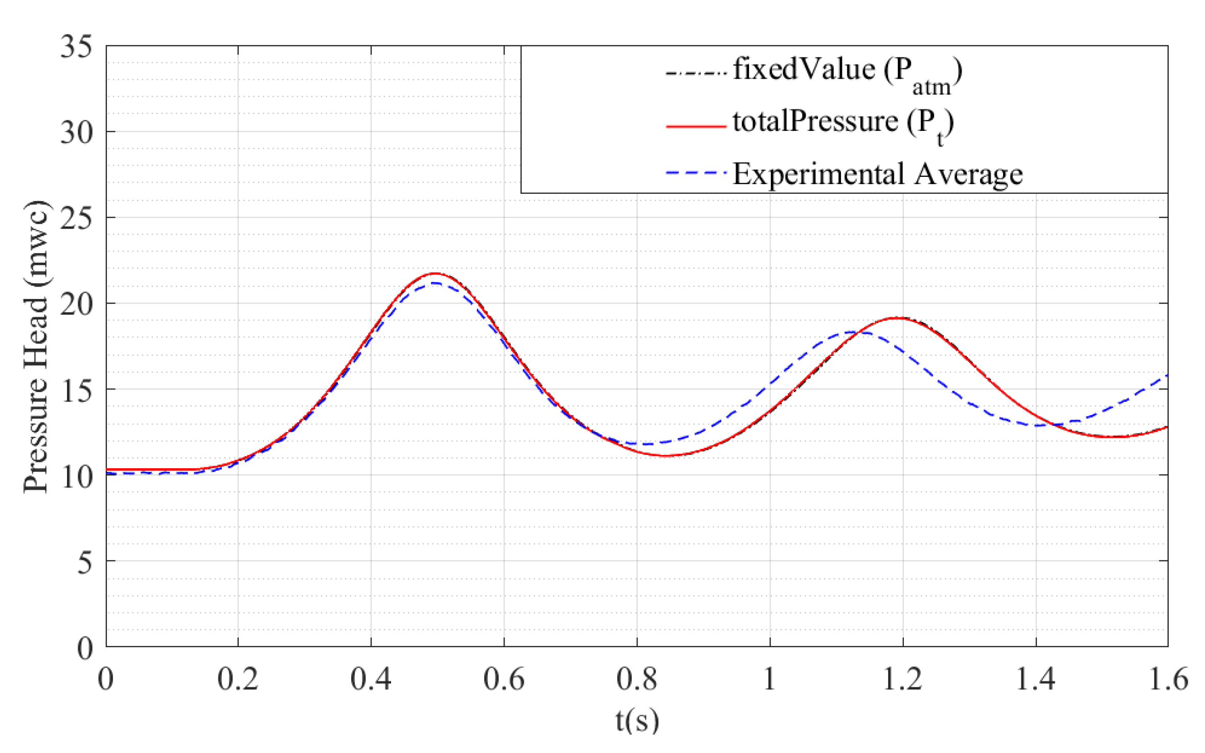
4.1. CFD Model Validation

For the 2D CFD model validation, the simulated patterns of pressure of the air pockets are compared with the experimental measurements (see Figure 4). The analysis of air pocket pressures under Experimental Tests No. 1 and 2, generated by the 2D model, does not show significant differences from the experimental data, both in extreme values and in wave oscillation patterns (see Figure 4a,b). According to the results, good adjustments of the air pocket pressure behaviour during the transient event are observed.

Figure 4. Comparison between the 2D CFD model and experimental tests.

When $P_i$ is higher ($P_i$ = 7.64 mwc), the determination of peak pressure loses reliability. For Experimental Test No 3, there is no practical evidence of significant differences in the first overpressure peak. On the other hand, for Experimental Test No. 5, the maximum pressure value of the air pocket that the simulation obtained is 30.20 mwc and the measured one is 29 mwc (see Figure 4c,e). The 2D model maximum pressure results during the first peak pressure of the hydraulic transient presented maximum differences of 2.43 mwc, with maximum relative errors of less than 9.1% and minimum of 0.71%, which are acceptable errors in the comparison between experimental and CFD model results [24]. Maximum pressures simulated by the 2D model ($P_{max.CFD}$) make a highly approximate match to the maximum experimental pressures ($P_{max.Exp}$) (see Table 3).

Table 3. Results of the CFD model $P_{max}$ CFD vs. Experimental data $P_{max}$.

Experimental Test	Experimental Repetition	${\mathit{P}}_{\mathit{max}.\mathit{Exp}}$ (mwc)	${\mathit{P}}_{\mathit{max}.\mathit{CFD}}$ (mwc)	% Experimental Error
1	1	15.10	13.73	9.10
1	2	14.98	13.73	8.38
2	1	15.24	14.33	5.95
2	2	15.04	14.33	4.72
3	1	21.30	21.45	0.71
3	2	21.65	21.45	0.91
4	1	21.35	22.24	4.18
4	2	21.65	22.24	2.72
5	1	29.65	30.20	1.98
5	2	29.08	30.20	3.84
6	1	29.05	31.65	8.91
6	2	29.18	31.65	8.43

The results of the 2D CFD model were compared to the mathematical model results presented by [16] where both models represented peak pressures adequately. The 2D CFD model makes a more precise simulation of the pressure oscillation during the transient hydraulic event compared to the mathematical model. In Figure 5, the comparison between these two models is exposed.

Figure 5. Behaviour of p in the air pocket during the filling process throughout its complete release.

As mentioned in [25], entrapped air pockets along non-straight pipes often lead to a more complicated interaction between air and water and more complex thermal issues. Furthermore, in 2D models, the deformation of air pockets in the 3rd dimension is not represented. Both hypotheses could explain the differences between the CFD model and the experimental one after the first peak.

4.2. Influence of the Boundary Conditions

The length of the outlet slot representing the 2D air valve behaviour was modeled using the aspect ratio $R_a$, which depends on the ratio of the air valve diameter to the pipe diameter, multiplied by an adjustment factor, which takes values between 0.3 and 1.0. The applied equation is given by:

$$L_r=R_a{D}_v=\left(\frac{D_v}{D_t}\alpha \right)D_v$$

(14)

where $Lr$ is the length of the slot; $R_a$ is a geometric aspect ratio; $\alpha$ is an adjustment coefficient; and $D_v$ and $D_t$ are the air valve diameter and the inner diameter of the pipeline, respectively. Table 4 shows the influence of the geometric aspect ratio of Experimental Test 5, considering different adjustment factors.

Table 4. $R_a$ influence over $L_r$ and the peak pressure. Experimental Test 5.

$\mathit{\alpha }$	${\mathit{L}}_{\mathit{r}}$ (mm)	${\mathit{P}}_{\mathit{max}}$ (mwc)	% Experimental Error
0.30	0.0588	42.61	30.5
0.50	0.0981	30.77	3.76
0.70	0.1373	30.65	3.38
0.88	0.1726	30.60	3.38
0.90	0.1765	30.38	2.54
0.92	0.1804	30.35	2.44
0.95	0.1863	30.31	2.30
1.00	0.1961	30.36	2.44

The use of a geometric aspect ratio is useful to ensure an equivalent mass flow for the two-dimensional modeling. For the assessed models, $\alpha$ values lower than 0.5 were found to increase the experimental error rate obtaining higher values than in experimental measurements. For $\alpha$ values between 0.9 and 1.0, the phenomenon is properly captured. That is why this is considered the most suitable range for the selection of the aspect ratio values for the 2D model configuration.

On the other hand, the following outlet conditions were considered for the 2D model using OpenFOAM: fixedValue, totalPressure. The fixedValue condition sets the outlet fixed pressure value at atmospheric ($P_{atm}$). TotalPressure defines the outlet pressure value as $P_t=P_{atm}-{\displaystyle \frac{1}{2}}\rho {\left|U\right|}^2$, where $P_{atm}$ is the atmospheric pressure (101,325 Pa). The $P_{atm}$ condition was employed for the adequate representation of the absolute pressure evolution of the air pocket in the simulations (see Figure 6).

Figure 6. Influence of the outlet boundary condition over the behaviour of the air pocket.

Based on the results in Figure 6, the boundary conditions associated with a fixed value pressure condition equal to the atmospheric pressure at the outlet boundary guarantees the same behaviour of the air pocket pressure inside the geometric domain as when using a total pressure boundary condition.

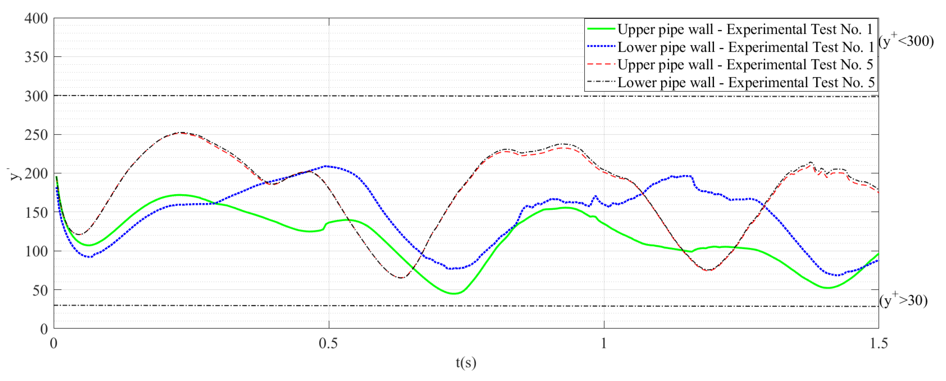
4.3. Near-Wall Flow Representation

In the present research, a refined mesh to the near-wall region was developed through the integration of the wall functions to derive the velocity profile. In the analysis, the $y^{+}$, variable was defined as the non-dimensional distance from the wall towards the pipeline interior. Figure 7 shows the results of $y^{+}$ in the Experimental Tests 1, 3, and 5. There, the model presents an acceptable range between 30 and 300 for the turbulent processes simulation, which is an adequate range for evaluation of the non-dimensional distance [26].

Figure 7. $y^{+}$ on the computational domain.

As proposed in [27], the cell size was determined based on the desired values of $y^{+}$. Unlike the conclusions reached in [27], the wall functions adequately modeled the phenomenon.

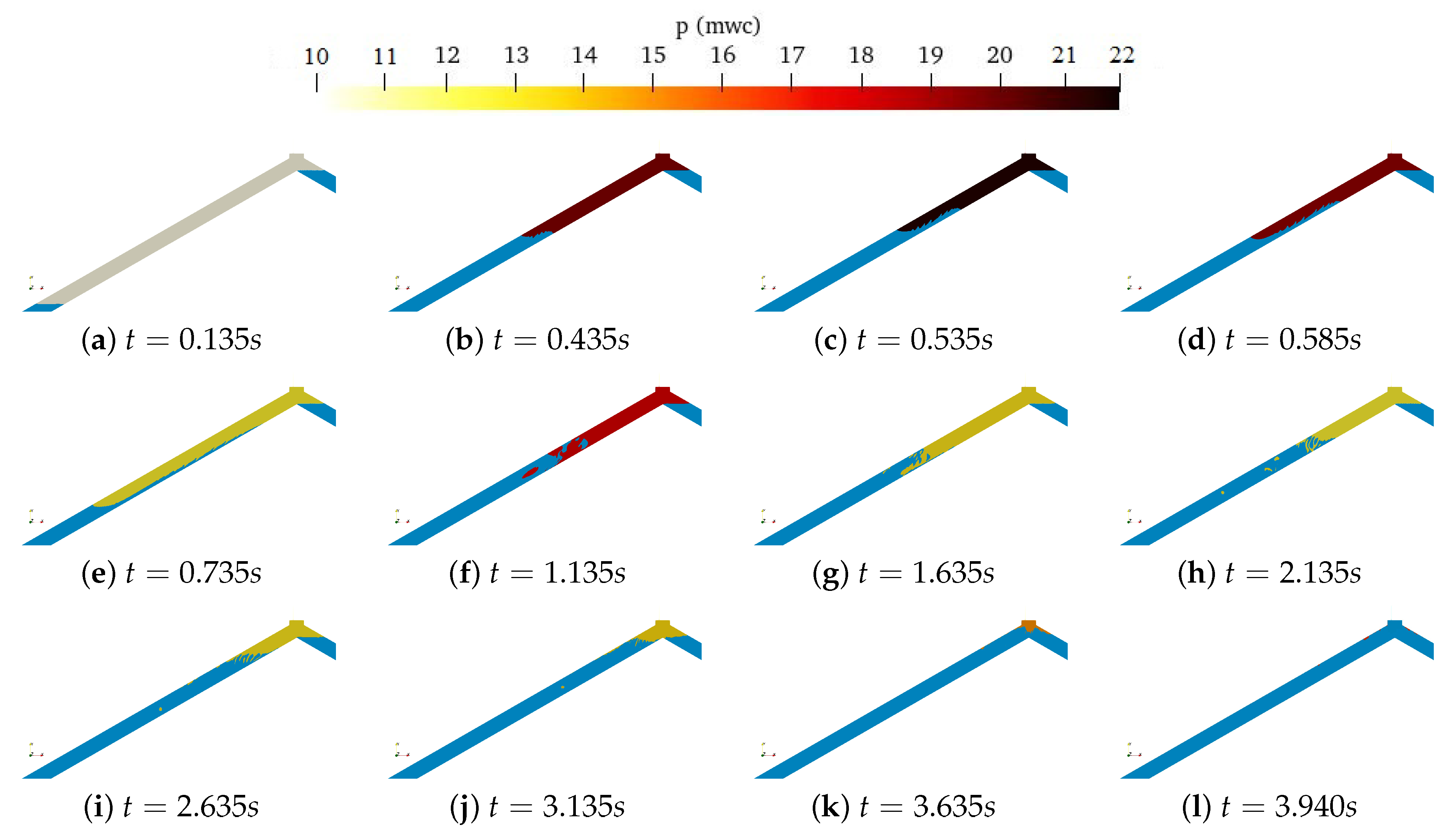
4.4. Air–Water Interface and Overpressure Analysis

The pipeline filling process time was examined for Experimental Test No. 3. The total time measurement of the filling process was 4 s. The 2D CFD model made possible to establish the filling time in 3.94 s, with a difference of only 1.5% regarding the experimental measurements. Figure 8 shows the different time steps in which the pipeline filling is occurring.

Figure 8. Behaviour of p in the air pocket during the filling process throughout its complete release.

Figure 8 shows that the water column occupies the interior of the pipeline, compressing the air pocket and allowing the expulsion of the air, resulting in the first peak of overpressure at a time of 0.53 s. However, a progressive expansion is generated with the need to release the compression energy accumulated in the air pocket, between the time instants t = 0.535 s to t = 0.735 s, resulting in a pressure drop of the air pocket. Subsequently, at time instant t = 1.135 s, a second overpressure peak is generated, due to the constant thrust of the water column on the air pocket, which expands again up to time instant t = 1.635 s. This phenomenon is progressive until the expulsion of the air pocket.

5. Conclusions

In the present study, a rapid water filling process using an air valve was simulated via a two-dimensional, compressible and multi-stage model on OpenFOAM. The compressible InterFoam solver worked on the governing equations of the phenomenon and the VOF method captured the air–water interface. The k-ω SST (Shear Stress Transport) turbulence model, and wall functions were chosen for the turbulence and high velocity gradient modeling. The air valve was simplified using the aspect ratio length shortening for the outlet slot, and the iteration cycles were set at a max. 1 × 10⁻⁶ s, with a fixed Courant number equal to 0.47. The 2D model results show that the OpenFOAM computational tool and the implemented solver enables to achieve adequate configurations for coherent results to represent and analyze this type of processes.

Within the conducted analysis to define the ideal configuration some conclusions emerged:

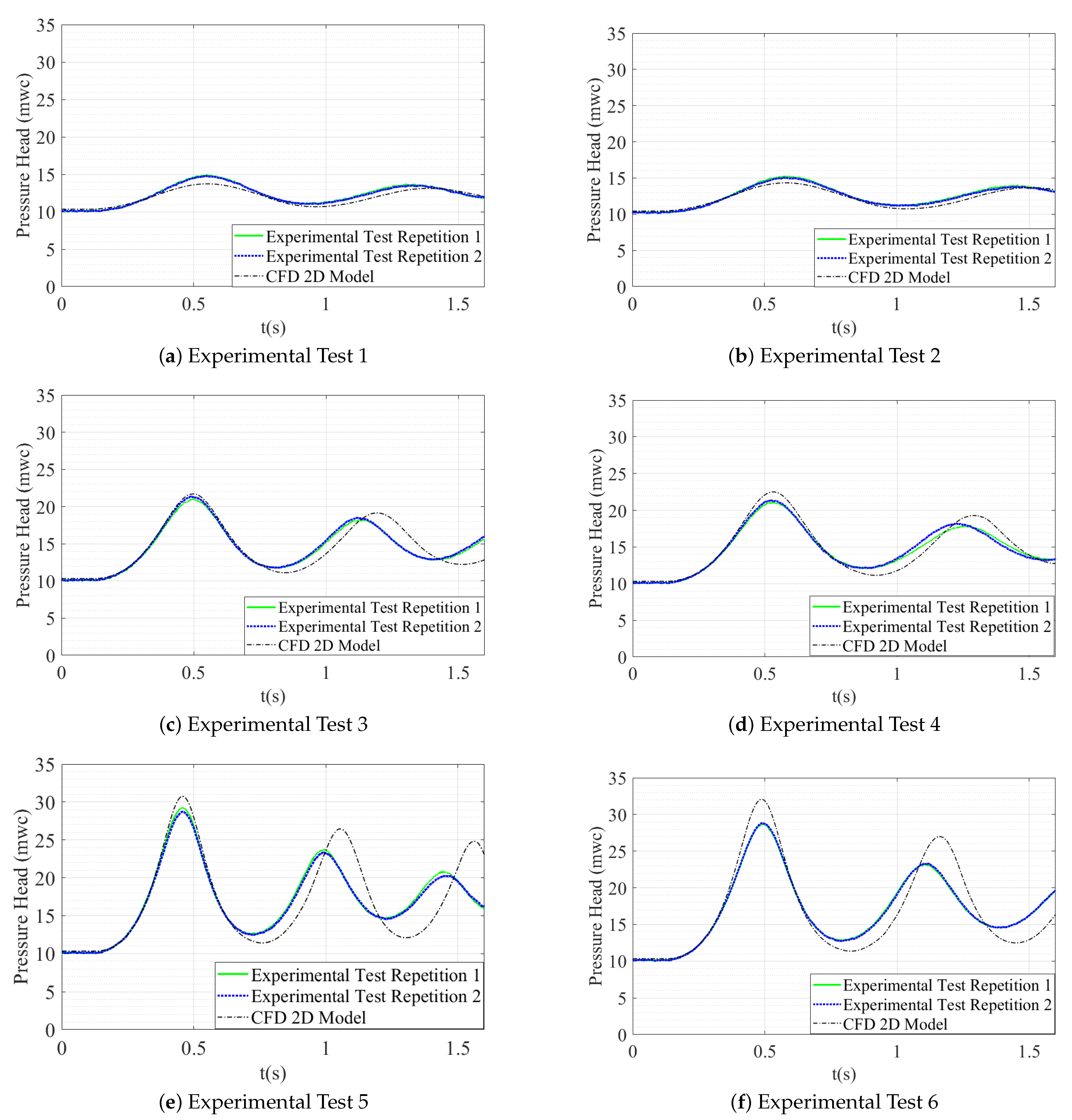
• The results of the first overpressure peak were well adjusted to the experimental tests, presenting experimental errors between 0.71% and 9.10%, which represents a good results from the numerical point of the view.
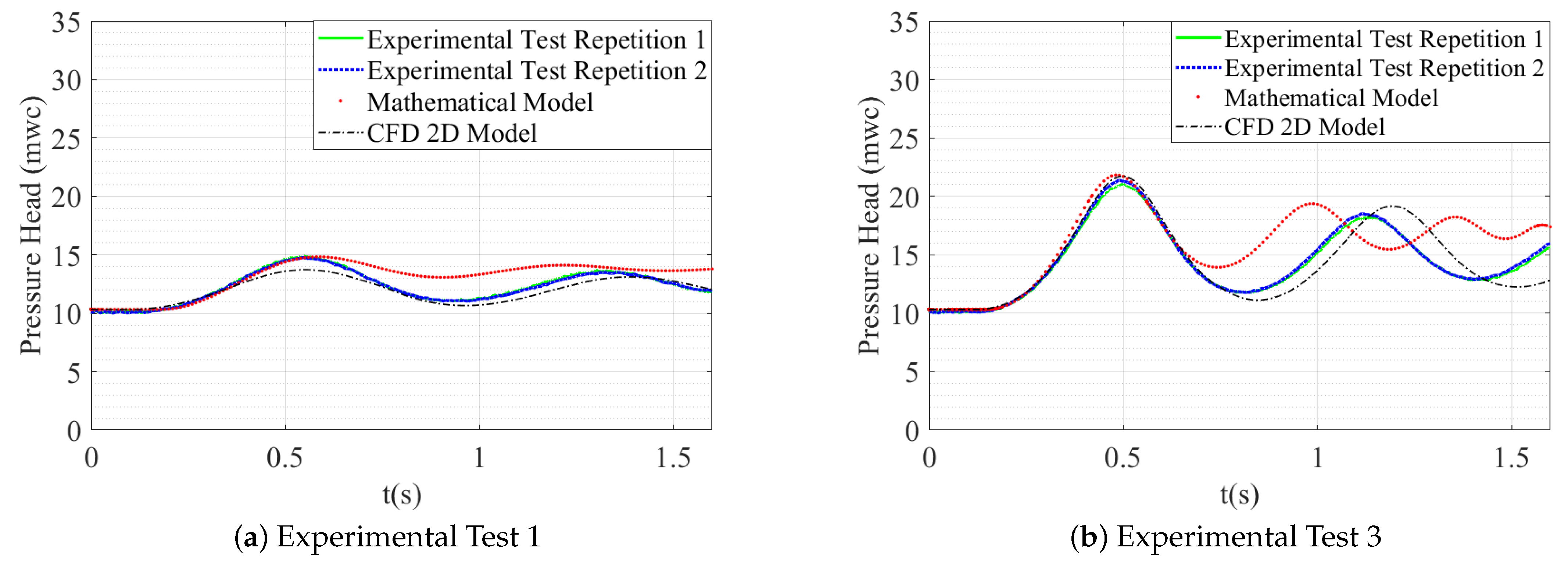
• In contrast to the mathematical models, the CFD models adjust very well with the pressure patterns of the respective experimental tests, this is evidenced in the pressure patterns of the CFD models and the mathematical model, after the formation of the first overpressure peak in the different cases (Figure 5).
• If aspect-ratio is not used to guarantee the system equivalence between the outlet of the air valve and the 2D modeled pipeline, results will not necessarily match the experimental data.
• The use of wall functions for turbulent layer modeling reduces the computational effort, managing to correctly simulate the phenomenon.
• The values of $y^{+}$ must remain in the range recommended by previous studies, given that if the cell size increases, the elements of the domain will not properly display the volume changes in the air pocket by either simulating lower values, or even matching the experimental ones but with longer wavelengths. An excessive refinement may result in pressure values higher than experimental values.
• The mesh refinement has a small influence on the wavelength; nevertheless, refining the mesh achieves complexity for maintaining $y^{+}$ within the defined range, demanding an extreme refinement, and managing to keep the height of the first cell inside the viscous layer, which is considered to be an unnecessary effort due to the coherent results obtained using wall functions.

References

- Fuertes-Miquel, V.S.; Coronado-Hernández, O.E.; Iglesias-Rey, P.L.; Mora-Meliá, D. Transient phenomena during the emptying process of a single pipe with water–air interaction. J. Hydraul. Res. 2019, 57, 318–326. [Google Scholar] [CrossRef]
- Fuertes-Miquel, V.S.; Coronado-Hernández, O.E.; Mora-Meliá, D.; Iglesias-Rey, P.L. Hydraulic modeling during filling and emptying processes in pressurized pipelines: A literature review. Urban Water J. 2019, 16, 299–311. [Google Scholar] [CrossRef]
- Hou, Q.; Tijsseling, A.S.; Laanearu, J.; Annus, I.; Koppel, T.; Bergant, A.; Vučković, S.; Anderson, A.; van’t Westende, J.M. Experimental investigation on rapid filling of a large-scale pipeline. J. Hydraul. Eng. 2014, 140, 04014053. [Google Scholar] [CrossRef] [Green Version]
- Malekpour, A.; Karney, B.; Nault, J. Physical understanding of sudden pressurization of pipe systems with entrapped air: Energy auditing approach. J. Hydraul. Eng. 2016, 142, 04015044. [Google Scholar] [CrossRef] [Green Version]
- Martins, N.M.; Delgado, J.N.; Ramos, H.M.; Covas, D.I. Maximum transient pressures in a rapidly filling pipeline with entrapped air using a CFD model. J. Hydraul. Res. 2017, 55, 506–519. [Google Scholar] [CrossRef]
- Zhou, L.; Liu, D.; Karney, B. Investigation of hydraulic transients of two entrapped air pockets in a water pipeline. J. Hydraul. Eng. 2013, 139, 949–959. [Google Scholar] [CrossRef]
- Fuertes, V. Hydraulic Transients with Entrapped Air Pockets. Ph.D. Thesis, Department of Hydraulic Engineering, Polytechnic University of Valencia, Valencia, Spain, 2001. Editorial Universitat Politècnica de València. [Google Scholar]
- Fuertes-Miquel, V.S.; López-Jiménez, P.A.; Martínez-Solano, F.J.; López-Patiño, G. Numerical modelling of pipelines with air pockets and air valves. Can. J. Civ. Eng. 2016, 43, 1052–1061. [Google Scholar] [CrossRef] [Green Version]
- Izquierdo, J.; Fuertes, V.; Cabrera, E.; Iglesias, P.; Garcia-Serra, J. Pipeline start-up with entrapped air. J. Hydraul. Res. 1999, 37, 579–590. [Google Scholar] [CrossRef]
- Liou, C.P.; Hunt, W.A. Filling of pipelines with undulating elevation profiles. J. Hydraul. Eng. 1996, 122, 534–539. [Google Scholar] [CrossRef]
- Liu, D.; Zhou, L.; Karney, B.; Zhang, Q.; Ou, C. Rigid-plug elastic-water model for transient pipe flow with entrapped air pocket. J. Hydraul. Res. 2011, 49, 799–803. [Google Scholar] [CrossRef]
- Zhou, L.; Pan, T.; Wang, H.; Liu, D.; Wang, P. Rapid air expulsion through an orifice in a vertical water pipe. J. Hydraul. Res. 2019, 57, 307–317. [Google Scholar] [CrossRef]
- Zhou, L.; Liu, D.; Karney, B.; Wang, P. Phenomenon of white mist in pipelines rapidly filling with water with entrapped air pockets. J. Hydraul. Eng. 2013, 139, 1041–1051. [Google Scholar] [CrossRef]
- Pozos-Estrada, O.; Fuentes, O.; Sánchez, A.; Rodal, E.; De Luna, F. Análisis de los efectos del aire atrapado en transitorios hidráulicos en acueductos a bombeo. Rev. Int. Métod. Numér. Para Cálculo Dise No Ing. 2017, 33, 79–89. [Google Scholar] [CrossRef] [Green Version]
- Romero, G.; Fuertes-Miquel, V.S.; Coronado-Hernández, Ó.E.; Ponz-Carcelén, R.; Biel-Sanchis, F. Analysis of hydraulic transients during pipeline filling processes with air valves in large-scale installations. Urban Water J. 2020, 17, 568–575. [Google Scholar] [CrossRef]
- Coronado-Hernández, Ó.E.; Besharat, M.; Fuertes-Miquel, V.S.; Ramos, H.M. Effect of a commercial air valve on the rapid filling of a single pipeline: A numerical and experimental analysis. Water 2019, 11, 1814. [Google Scholar] [CrossRef] [Green Version]
- Ahadzadeh, N.; Tabesh, M. Application of two-component pressure approach and harten–lax–van leer (hll) solver to model transient flow with regard to air entrapment. Water Sci. Technol. 2020, 81, 596–605. [Google Scholar] [CrossRef] [PubMed]
- Besharat, M.; Tarinejad, R.; Aalami, M.T.; Ramos, H.M. Study of a compressed air vessel for controlling the pressure surge in water networks: Cfd and experimental analysis. Water Resour. Manag. 2016, 30, 2687–2702. [Google Scholar] [CrossRef]
- Zhou, L.; Liu, D.-Y.; Ou, C.-Q. Simulation of flow transients in a water filling pipe containing entrapped air pocket with vof model. Eng. Appl. Comput. Fluid Mech. 2011, 5, 127–140. [Google Scholar] [CrossRef] [Green Version]
- Liu, D.; Zhou, L. Numerical simulation of transient flow in pressurized water pipeline with trapped air mass. In Proceedings of the 2009 Asia-Pacific Power and Energy Engineering Conference, Wuhan, China, 28–30 March 2009; pp. 1–4. [Google Scholar]
- Greenshields, C. OpenFOAM: The Open Source CFD Toolbox; OpenFOAM Foundation Ltd.: London, Uk, 2015. [Google Scholar]
- Hernandez-Perez, V.; Abdulkadir, M.; Azzopardi, B. Grid generation issues in the cfd modelling of two-phase flow in a pipe. J. Comput. Multiph. Flows 2011, 3, 13–26. [Google Scholar] [CrossRef]
- Salim, S.M.; Cheah, S. Wall y strategy for dealing with wall-bounded turbulent flows. In Proceedings of the International Multiconference of Engineers and Computer Scientists, Hong Kong, China, 18–20 March 2009; Volume 2, pp. 2165–2170. [Google Scholar]
- Wang, H.; Zhai, Z.J. Analyzing grid independency and numerical viscosity of computational fluid dynamics for indoor environment applications. Build. Environ. 2012, 52, 107–118. [Google Scholar] [CrossRef]
- Zhou, L.; Wang, H.; Karney, B.; Liu, D.; Wang, P.; Guo, S. Dynamic behavior of entrapped air pocket in a water filling pipeline. J. Hydraul. Eng. 2018, 144, 04018045. [Google Scholar] [CrossRef]
- Gersten, K. Hermann schlichting and the boundary-layer theory. In Hermann Schlichting—100 Years; Springer: Berlin/Heidelberg, Germany, 2009; pp. 3–17. [Google Scholar]
- Shukla, I.; Tupkari, S.; Raman, A.; Mullick, A. Wall y plus approach for dealing with turbulent flow through a constant area duct. AIP Conf. Proc. 2012, 1440, 144–153. [Google Scholar]
Publisher’s Note: MDPI stays neutral with regard to jurisdictional claims in published maps and institutional affiliations. |
© 2021 by the authors. Licensee MDPI, Basel, Switzerland. This article is an open access article distributed under the terms and conditions of the Creative Commons Attribution (CC BY) license (https://creativecommons.org/licenses/by/4.0/).