Article

On Dam Failure Induced Seismic Signals Using Laboratory Tests and on Breach Morphology due to Overtopping by Modeling

1
Department of Soil and Water Conservation, National Chung Hsing University, Taichung 40227, Taiwan
2
Innovation and Development Centre of Sustainable Agriculture (IDCSA), National Chung Hsing University, Taichung 40227, Taiwan
*
Author to whom correspondence should be addressed.
Water 2021, 13(19), 2757; https://doi.org/10.3390/w13192757
Submission received: 22 August 2021 / Revised: 27 September 2021 / Accepted: 1 October 2021 / Published: 5 October 2021
(This article belongs to the Special Issue Soil–Water Conservation, Erosion, and Landslide)

Abstract

:
Dam models were constructed in an indoor flume to test dam breach failure processes to study the seismic signals induced. A simple dam breach model was also proposed to estimate hydrographs for dam breach floods. The test results showed that when the retrogressive erosion due to seepage of the dam continues, it will eventually reach the crest at the upstream side of the dam, and then trigger overtopping and breaching. The seismic signals corresponding to the failure events during retrogressive erosion and overtopping of the dam models were evaluated. Characteristics of the seismic signals were analyzed by Hilbert–Huang transform. Based on the characteristics of the seismic signals, we found four types of mass movement during the retrogressive erosion process, i.e., the single, intermittent, and successive slides and fall. There were precursor seismic signals found caused by cracking immediately before the sliding events of the dam. Furthermore, the dam breach modeling results coincided well with the test results and the field observations. From the test and modeling results, we confirmed that the overtopping discharge and the lateral sliding masses of the dam are also among the important factors influencing the evolution of the breach. In addition, the widening rate of the breach decreases with decreased discharge. The proposed dam breach model can be a useful tool for dam breach warning and hazard reduction.

1. Introduction

Large landslides induced by rainfall or earthquakes may form landslide dams and inundate upstream areas. If the dam breaches, it will pose a serious threat to the area downstream. Nearly 89% of landslide dam failures are caused by overtopping [1,2]. The large-scale landslide caused by Typhoon Morakot in 2009 in Xiaolin village in southern Taiwan caused over 400 fatalities. It also formed a landslide dam [3,4,5]. Feng (2012) [6] indicated that the dam breached 1 h and 24 min after its formation according to the seismic signal recorded and the time–frequency spectrum. They estimated the velocity of flood propagation downstream to be 8.3 m/s. The dam breach produced large turbulent flows downstream in a short period of time, causing flooding downstream and the failure of many bridges.
In 1951, heavy rainfall caused a large-scale landslide in Tsaoling, Yunlin County, Taiwan, and a large landslide dam was formed. As a result, 137 army engineers unfortunately sacrificed their lives during the installation of an emergency spillway due to the sudden overtopping failure of the dam [7]. In 1999, a large landslide occurred in Tsaoling again due to the 1999 Chichi earthquake [8]. Five landslide-dammed lakes were subsequently formed, of which three were cleared soon after the landslide. However, the other two were not easily cleared, so were strengthened to improve the stability of the dam and emergency spillways were setup to prevent overtopping erosion [9]. Due to the establishment of emergency spillways that controlled the maximum water storage capacity of the landslide dam, the impacts of four typhoons (Typhoon Bilis in 2000, Torajiin 2001, Nari and Mindulle in 2004) were reduced [10]. Cui et al. (2013) [11] and Zhou et al. (2015) [12] reported that on 8 August 2010, the intense rainfall and cascading failure of landslide dams along two gullies induced a fatal debris flows to Zhouqu County, China, that claimed the lives of 1765 people and damaged infrastructure and many homes. Their preliminary field and experimental studies showed that landslide dam cluster modes (i.e., different dam types and their combination) in upstream gullies accounted for the amplification of the scale of Zhouqu debris flows downstream. Cai et al. (2019) [13] analyzed the cascade dam system using a dam breach analysis model (DB-IWHR) for continuous breaking failure paths. They also created a Bayesian network model to determine the failure probability of the cascade dam system. Říha et al. (2020) [14] also modeled cascade dams and indicated that the peak discharge of a dam cascade system may be underestimated by up to 10% when applying an empirical formula derived for a single dam breach. Shrestha and Nakagawa (2016) [15] studied the large-scale landslide in Nepal that resulted from heavy rainfall on 2 August 2014 and the landslide dam on the Sunkoshi River. The retained water overflowed 36 days after the landslide. However, there was no serious damage downstream and no casualties because an emergency spillway was setup before the overflow and the spillway controlled the overflowing water. From these reviews, it is clear that landslides and dam breaches can cause a large number of casualties and property destruction. Therefore, research on the failure processes of landslide dams and hazard prevention of landslide dams is very important.
Hazard prevention and monitoring of landslide dams are always compulsory. Many scholars have used seismic signals recorded from geophones and/or accelerometers for analyses for the creation of warning systems [16,17,18,19,20]. Because both landslide and dam breach events generate seismic signals, the signals can be faithfully recorded by seismometers, and so can be used for interpreting the processes of landslides and dam breach events. However, the seismic signals of landslide and dam breach events cannot always be successfully recorded due to limitations. Additionally, because natural phenomena cannot be repeated, a series of event data cannot be obtained for analysis. Therefore, researchers have often adopted numerical simulations, outdoor large-scale experiments, and indoor small-scale experiments to conduct research on seismic signals induced by landslide dam failure.
Yan et al. (2020) [21] reconstructed the dynamic behavior of the 2017 landslide event in Xinmo village, China, by using the seismic signal characteristics and discrete element method. They categorized the landslide processes into five stages: stationary, slipping, transition, entrainment–transportation, and deposition stages, according to the characteristics of the seismic signals and time–frequency spectra. They identified the transition stage, which is caused by ancient colluvial materials hindering sliding from upslope. However, as the sliding materials continued to accumulate and produce more downward dragging forces, another larger landslide was triggered. This can be observed from the seismic signal as the amplitude first decreases and then increases at the transition stage. Feng et al. (2017) [22] used PFC coupled with FLAC to simulate the 2009 Xiaolin Village landslide process and compared the results with the seismic signal recorded by a broadband seismometer. They found that the types of movement and terrain significantly affect the seismic signal. Although a numerical simulation can readily reconstruct the failure process and influence zones of a landslide, sometimes it is not easy to select accurate physical parameters; thus, the simulation results may be different from the actual landslide.
Some researchers also choose large-scale outdoor experiments. Yan et al. (2017) [23] monitored the seismic signals generated during an outdoor dam-breach test. According to their results based on time–frequency analysis, the low-frequency band (0–1.5 Hz) was mainly due to dam collapse events; the intermediate-frequency band (1.5–10 Hz) was due to rock slide events; the high-frequency band (10–45 Hz) was a result of water flow and sediment transport. Feng et al. (2020a) [24] conducted a large-scale dam breach test at Huisun Forest Station in Nantou, Taiwan. They discussed the characteristics of seismic signals during the dam breach processes and flooding. The flood speed of the test was also estimated from the seismic signals. They indicated that seismic signals can be applied as a basis for early warnings for floods. As we know, a large-scale outdoor test better reflects natural dam breach behavior than the numerical simulation and the small-scale indoor flume test. However, due to the limitations of outdoor large-scale tests that require a large area, long preparation time, and are relatively more expensive, they are less widely used than indoor flume tests.
Many researchers use small indoor flumes to perform tests for landslide dam breaches [25,26,27,28]. Most of the tests explored the erosion of the dam body, including the effects of different flume slopes, dam geometry, and material properties. However, the seismic signals caused by the destruction of the dam are less discussed. Hu et al. (2018) [29] used a small flume to test the seismic signals of internal dam erosions. They found a precursor seismic signal prior to the sliding of dam materials. Seismic signals caused by internal erosion due to seepage were mainly high-frequency. If the dam materials were loosely packed, there were more high-frequency seismic signals induced due to the internal erosion. However, they only discussed the seismic signals of dam failure due to seepage and did not discuss the overtopping dam breach and subsequent flooding. There are seismic precursors detected prior to landslides reported in the literatures, e.g., Poli (2017) [30] and Butler (2019) [31]. Feng et al. (2020b) [32] used an indoor flume to study the seismic signals of landslides caused by riverbank erosion. They also found precursor seismic signals before the riverbank sliding. They classified the river bank sliding into three types: single, intermittent, and successive. The three types correspond to the three different characteristics of seismic signals. They also pointed out that the higher frequency seismic signal decays faster than the lower frequency signal. However, this research did not perform tests for retrogressive erosion of a dam due to seepage and overtopping failure.
This research performed tests for retrogressive erosion of a dam due to seepage and the subsequent overtopping failure of dam models. A theoretical dam breach model was proposed and used to compare the flooding process of the test. The experimental setup was a modified version of the test used by Feng et al. (2020b) [32]. In the tests, accelerometers were installed inside the dam to monitor the seismic signals during the dam failure and to understand the correspondence between the failure processes and characteristics of the seismic signals. Hilbert–Huang transform [33] was used for time–frequency analysis for the seismic signals recorded. The setting of the test conditions in this study is not a simple overtopping failure but is similar to the progressive (retrogressive) failure of an outdoor dam breach test by Takayama et al. (2021) [34]. The progressive failure was mainly induced when the dam body was retrogressively eroded towards the upstream crest by seepage. Initially, only small slides and erosions occurred at the toe of the slope, and then as the phreatic surface of the seeping water gradually rose, an increasing number of slides and erosions occurred from the toe towards the crest. At this point, overtopping occurs and the dam starts to breach with vertical downcutting and lateral erosion. The overtopping flood gradually expands the width of the breach, and then a larger amount of floodwater is discharged downstream.
During overtopping, the breach is widened and deepened by the overflowing water. To model the dam breach process, Wu (2011) [35] listed different model approaches and pointed out that modeling can be classified as: (1) parametric breach models and (2) physically based breach models. Parametric breach models usually use statistical regression equations based on laboratory experiments or field dam failure cases. Physically based breach models were highly developed during the past decades and can simulate the dam breach process in a more complete and detailed way. However, the models require heavy numerical calculation requiring extensive calculation time. In addition, these detailed simulation models can be limited due to a lack of understanding of sediment transport under the flow conditions and require multiple runs to calibrate. Unlike the detailed simulation, Alhasan et al. (2015) [36] proposed a conceptual model, simplified the three-dimensional problem to a one-dimensional problem, and successfully compared the results with field observations. To simulate the horizontal expansion of the dam breach, Tian et al. (2021) [37] proposed a model to combine a theory of sediment transport for vertical incision and a horizontal expansion model based on geotechnical theory. Similarly, the framework proposed in this research is based on the simplified analytical dam breach model by Capart (2013) [38]. We considered the sediment mass conservation Exner equation [39] and a simple sediment transport law [40] to describe the changing of the dam and channel bed profile. We then use this proposed dam breach model to predict the discharge, the height of the crest, and width of the breach for our test. Comparison and analyses were made between the dam breach model calculations and the test results to verify the feasibility of the model.
The major purposes of this study are to discuss (1) the seismic signal precursors prior to the sliding of the dam, (2) the types of movement of the sliding mass of the dam during the retrogressive erosion due to seepage, and (3) the dam breach model proposed and its comparison with the test results.
In this study, only the most representative test result was chosen for presentation; however, many tests were performed and similar results were obtained.

2. Materials and Methods

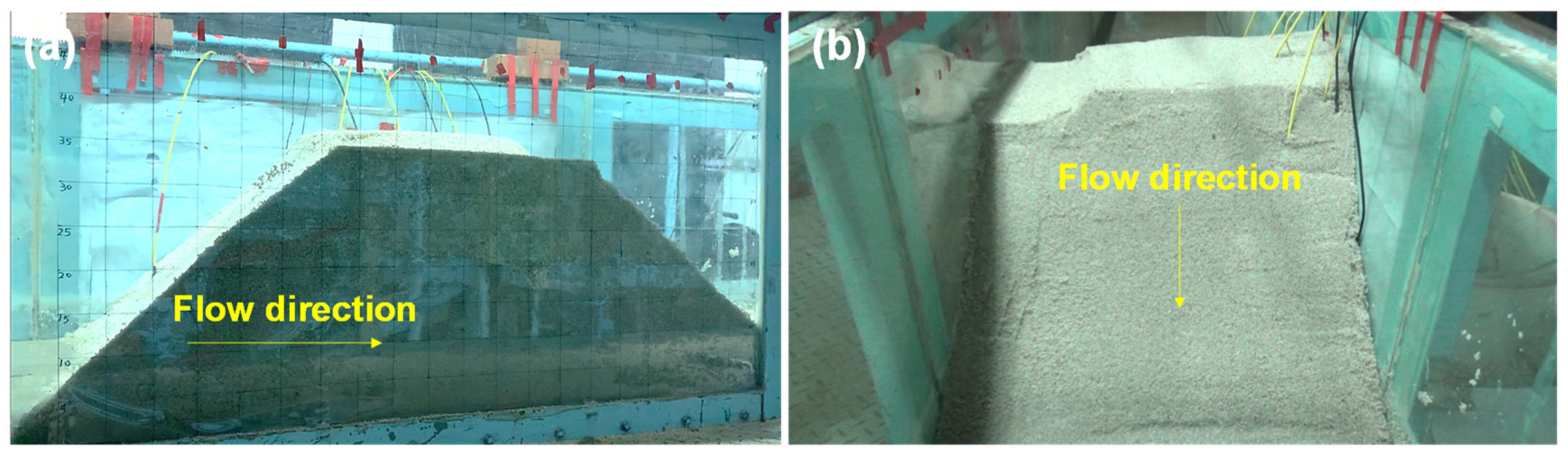
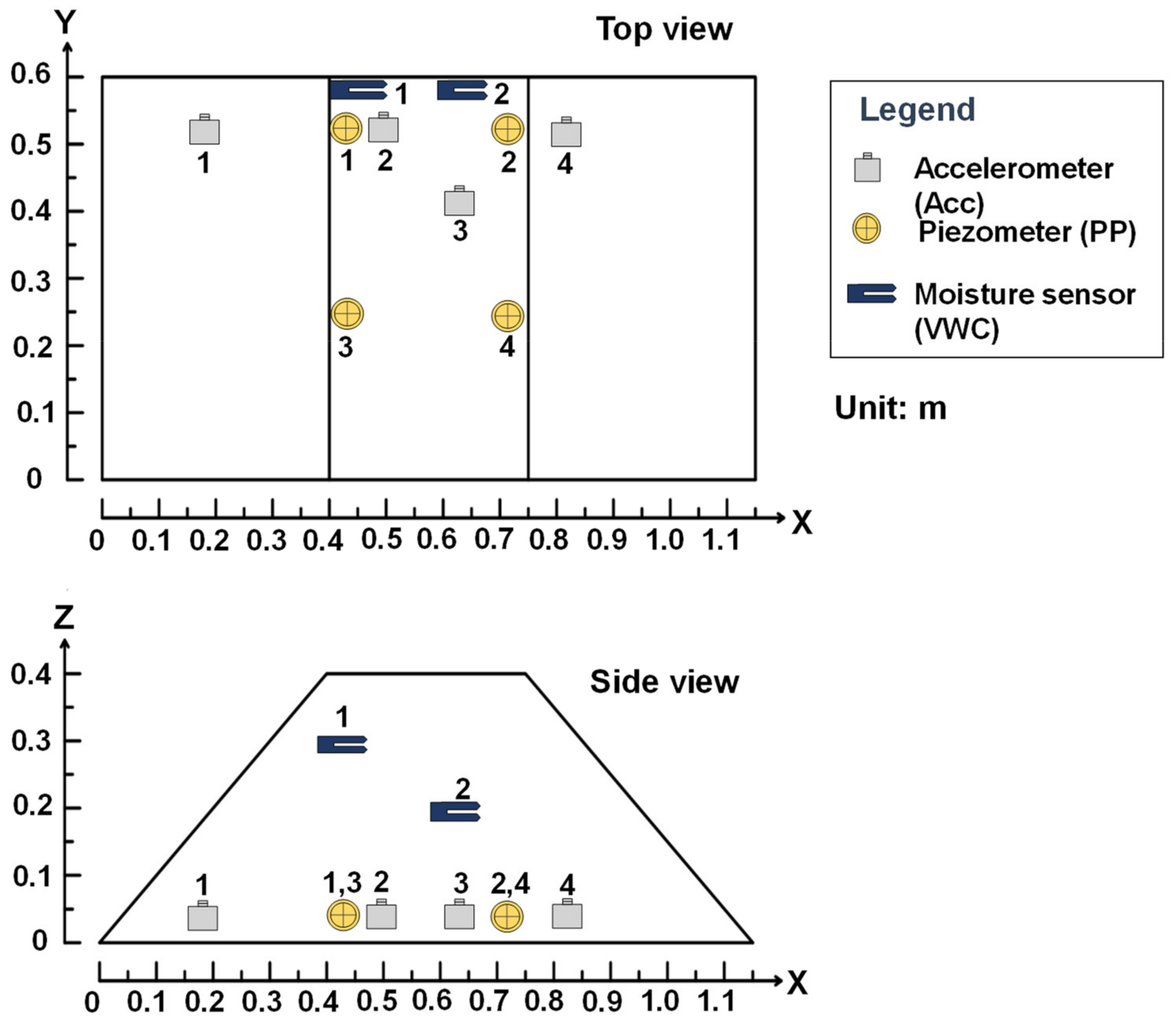
2.1. Test Configuration

The laboratory flume is shown in Figure 1, which is the same equipment used in Feng et al. (2020b) [32]. The size of the flume is 15 × 0.6 × 0.6 m and the slope of the channel bed is 0.1%. The pump is mainly used to pump water from the underground storage tank to the headwater. Water is introduced from the headwater into the water tank and controlled by a sluice (a valve). The inflow is regulated by a screening device before flowing into the flume channel to enable stable flow conditions. The design of the water supply setup is similar to that of Alhasan et al. (2016) [41] in that the water was stilled/regulated before entering the flume channel. Dimensions of the dam model are listed in Table 1. The slope of the dam is 1:1 (45°) before water impounding. After the construction of the dam model, it was left to sit for 1 h before the test. This study assumes that the right side of the flume is an axis of symmetry; therefore, an overflow notch of 0.05 m depth was set on the right side of the flume. The material used to construct the dam model was sieved uniform sand with a median particle diameter of D50 = 1.5 mm, D10 = 0.9 mm, and D90 = 12.1 mm. The unit weight of the dam material averaged 13.93 kN/m3 and the density of solid particles ρs = 2583 kg/m3. The void ratio was 0.816 and porosity 45%. The initial moisture content of the dam materials was measured as 5–8%. The initial internal friction angle of the dam material was estimated to be 38–40°. A sand bed with a length of 3.8 m and a thickness of 0.05 m was placed downstream of the dam (Figure 1). Figure 2 shows the side and front view of the dam model.
The dam model was instrumented with sensors including 4 accelerometers, 4 piezometers, and 2 moisture sensors. Figure 3 shows the configuration of the sensors in the dam model and are numbered for identification. The locations of the sensors were selected so that they are not washed out during the tests. Therefore, they were mostly installed on the left side of the dam, with the exception of PP-3 and PP-4. The piezometers were installed close to the bottom of the dam to reflect pore pressure. Moisture sensors 1 and 2 were installed higher, at 0.2 and 0.3 m above the bottom to detect when the seepage water reached those levels. The accelerometers were of the Type 731A produced by Wilcoxon Sensing Technologies with a response frequency between 0.1 and 450 Hz and sensitivity of 10 V/g. The sampling rate was set at 5.12 kHz for the accelerometers to record seismic signals. The piezometers were of the Type KPE-200KPB made by Tokyo Measuring Instruments Laboratory Co, Ltd., and were installed 3 cm above the bottom of the dam model to trace pore pressure (PP) variation during the test. The moisture sensors were of the Type EC-5 produced by METER Group, Inc., and were installed at two different levels to monitor variation in volumetric water content (VWC).
Three cameras were set up at the right side, front, and top of the dam model to record the test process. Because the shooting angle of the sideview file was skewed, for subsequent analyses we used a projection to estimate the water level changes and dam dimensions during the breach.
Brief test process: When water was released, the upstream water level gradually increased until the maximum water level was reached. The maximum water level was controlled by the sluice and maintained at 0.3 m until overtopping. The pump was turned off at 116 s for better seismic signal quality. At 130 s, a tapping was made to leave a time marker, which was used to match the time axis between seismic signals and the test videos. After water seeped into the dam and outflowed at the downstream toe, retrogressive erosion and landslides then started. When the retrogressive erosion reached the upstream crest of the dam, overtopping occurred. A breach was then formed, down cut, and widened. The detailed test process and results are discussed in Section 3.

2.2. Seismic Signal Processing by Hilbert–Huang Transform (HHT)

The seismic signals recorded during the tests were processed using Hilbert–Huang transform (HHT, Huang et al. 1998) [33]. HHT includes empirical mode decomposition (EMD) to calculate the intrinsic mode functions (IMFs) and a Hilbert transform (HT) to obtain the corresponding time–frequency spectra from the IMFs. HHT can process unsteady and nonlinear signals and analyze the relationship between time, seismic frequency, and energy distribution of signals. The HHT analyses in this study were performed by Visual Signal Ver. 1.6 software (AnCad, Inc. (2018) [42]). The characteristics of the seismic signals due to various sliding events can be identified more easily with the help of time–frequency spectra. The HHT was also applied in Feng et al. (2020b) [32] and Feng et al. (2020a) [24] to successfully interpret flood and landslide events.

2.3. Dam Breach Model—Overtopping

As we described in the previous section, the test can be separated into two stages. In the first stage, the seepage water flows out of the downstream surface of the dam, causing retrogressive erosion. Due to the retrogressive erosion, the shape of the dam deforms from a trapezoid to triangle and the breach process leads to the second stage. In the second stage, the water overtops the crest and begins the overtopping process. In the second stage, the outflow from the crest dominates the breach process and reduces the water level in the lake.
To simulate the overtopping incision process and compare it with the test results, we propose a simplified dam breach model based on Capart (2013) [38]. In this model, we neglect the discharge due to seepage and simulate the breaching as a continuous process. As illustrated in Figure 4, we assumed a triangular-shaped dam with upstream slope R D , downstream slope S D , and initial elevation of the dam z D ; z C t is the crest level and z L t is the lake level. The initial crest level z C t = 0 is equal to z D . The initial lake level z L t = 0 before overtopping is assumed to be maintained at a steady level.
The Exner equation governs the breach process based on the sediment mass balance (Paola and Voller 2005) [43].
b z t + J x = 0
where b is the channel width, z is the bottom elevation of the breach channel, x is the streamwise direction, and J is the sediment transport rate. In this equation, Paola and Voller (2005) [43] simply demonstrated the mass of bedload balancing in a controlled volume; when sediment influx J x is larger than outflux J x + Δ x the elevation of the sediment in the control volume increases. For the sediment transport rate, Visser (1995) [44], Alhasan et al. (2016) [41], and Haddadchi et al. (2013) [45] collected different empirical sediment transport formulas used in sand–dike breach erosion. The formulas were verified with experimental results or field cases. However, the formulas contained too many detailed variables and coefficients (e.g., internal friction coefficient, bed shear velocity), which increases the complexity of the model [46]. In the 1950s, Lane (1955) [40] presented a qualitative law of sediment transport rate, which demonstrated J can be generally scaled by the water flux and the channel gradient as:
J = K Q S = K Q z x
where K is a dimensionless transport coefficient; Q is the local discharge (the discharge through the breach); S is the channel gradient, which can be written as the derivative of channel elevation in the streamwise direction. By substituting (2) into (1), a variable rate diffusion equation can be obtained. Next, we assumed the outflow channel at the toe of the dam converges to the initial shape of the dam, and the level of the crest level evolves along with the water level of the lake. A zero-sediment flux is assumed at the crest ( J x C t , t = 0 ) as the second upstream boundary condition [47,48]. By defining operational time d τ t = K Q t / b , the varying rate diffusion equation can be reduced to a standard diffusion equation:
z τ 2 z x 2 = 0
For this dam breach problem (triangle dam with moving upstream boundary condition), a similar structure of the solution can be found in Capart et al. (2007) [47], Voller et al. (2004) [49], and Lai and Capart (2007, 2009) [50,51], and the detailed derivation can be found in Capart (2013) [38]. By using the boundary conditions, the profile of the dam was solved as:
z x , τ = z D S D x R D + S D λ s ierfc 0.5 λ s τ   ierfc 1 2 x / τ
where S D and R D represent the downstream slope and upstream slope of the dam, and ierfc( ξ ) is a special function introduced by Carslaw and Jaeger (1959) [52]:
ierfc ξ = ξ erfc x d x = 1 π e x p ξ 2 ξ e r f c ξ
where erfc ξ is the complementary error function and λ s is a constant related to the shape of the dam. By taking the upstream sediment flux boundary condition at the dam crest position, λ s can be solved numerically in Equation (6):
0.5 λ s   e r f c 0.5 λ s i e r f c 0.5 λ s S D S D + R D = 0  
Following the profile of the dam, focusing on the dam crest, the drop of crest δ τ can also be written as:
δ τ = z D z x C τ , τ = R D λ s τ
We replaced the operational time τ with the real time, and the time evolution of the breach drop can be given by the ODE:
d δ t d t = 1 2 K Q b R D 2 λ s 2 δ t
V E indicates the erosion volume at the crest during the overtopping process. Here, we find that V E can be scaled as the drop of the crest and the width of the width δ 2 b . To include the widening effect and simplify the governing equation, we rewrite the equation as:
d V E t d t = d d t δ 2 b = K T Q = K V + K L Q
where K T is the scaled coefficient of the total sediment transport coefficient; K L and K V represent the coefficients of the erosion rate of the dam in lateral and vertical directions, respectively. To separate the process of vertical incision and lateral erosion, we applied chain rules to simplify the partial differential equation (PDE) (Equation (9)) into two ordinary differential equations (ODEs):
d δ t d t = K V Q t 2 b t δ t d b t d t = K L Q t δ t 2
To simulate the lake drainage, the level-pool routing equation [53] is adopted:
A L d z L d t = Q
where A L is the lake area, which we assume constant during breaching. For the outflow discharge Q, the broad-crested discharge equation is used:
Q = 8 g 27 b η t 3 / 2
where η t = z L t z C t represents flow depth at the crest. By substituting the broad-crested-weir discharge equation (Equation (12)) into the level-pooling routing equation, Equation (11) can be rewritten as:
d η t d t = d δ t d t 1 A L 8 g 27 b η t 3 / 2
Now, the three ODEs (the two ODEs from Equation (10) and the ODE of Equation (13)) with the three variables, η t ,   δ t ,   and   b t , were successfully derived. The forward Euler method, a first-order numerical procedure for solving ODEs, was applied to calculate the solution of the dam breach model with the following initial conditions:
δ 0 = 0 ,   η 0 = 0 ,   b 0 = b 0
The water level of the lake is assumed to be the same height of the crest as the initial condition at t = 0, and b 0 is the initial channel width.
The proposed dam breach model is then successfully derived and can be solved numerically. This model is simple because we only have to solve the simpler ODEs instead of the PDEs. The model results were compared with the field observations from the literature and test result in Section 3.

3. Results and Discussions

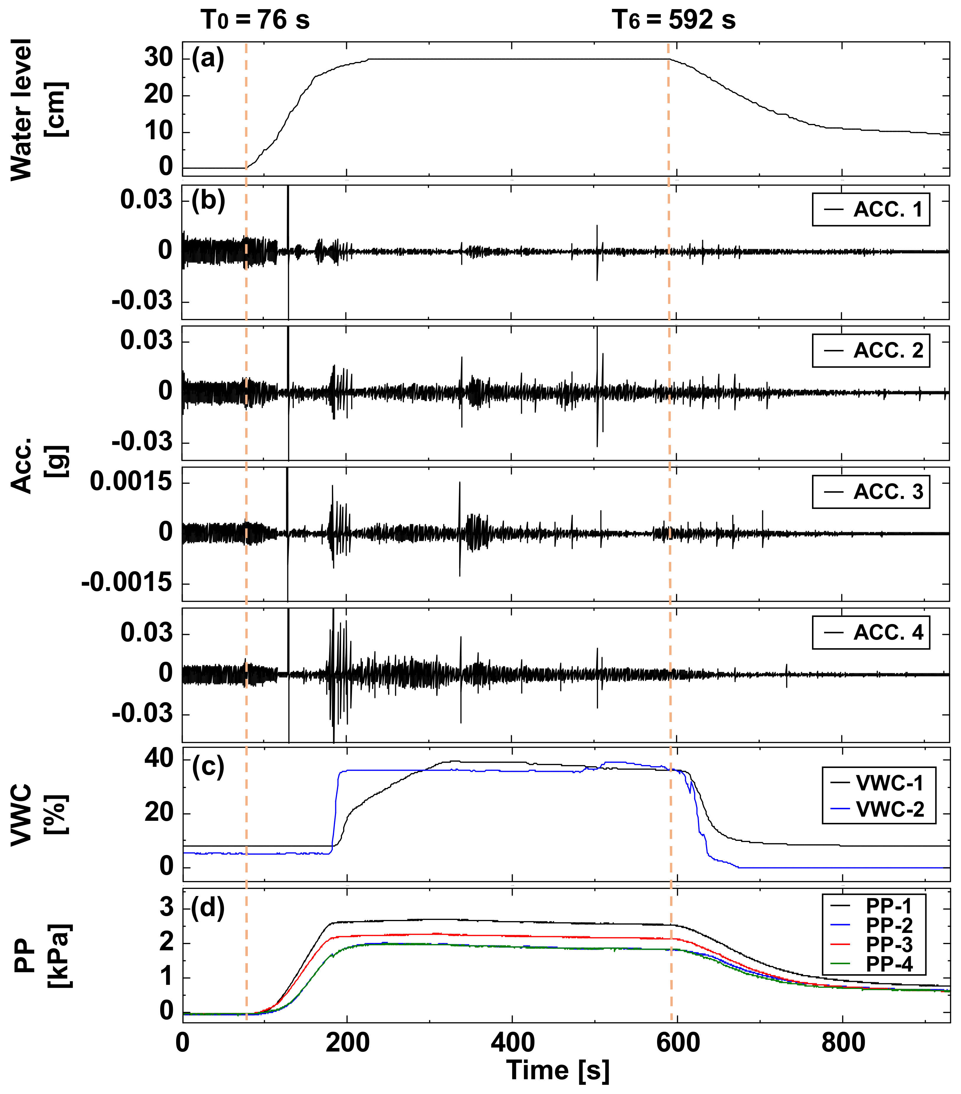
3.1. Measurements of the Test

In the discussion of the test results hereafter, the term “tank” was used instead of “lake”. They both represent the water level at the upstream side of the dam in this study. The test processes included tank level raising, water seeping into the dam, sliding of the dam due to retrogressive erosion, overtopping, breach downcutting, and widening and lateral sliding of the dam. Table 2 lists the timing, test stages, selected important events, and variation of the seismic signals of the test processes. We defined T0 = 76 s as the time when the upstream water reached the toe of the dam. Sliding Events 1–6 occurred between 180.6 and 231.9 s, of which Events 1–3 occurred during the rising of the tank level and Events 4–6 occurred when the tank level was maintained at 0.3 m. Events 1–6 are discussed in detail later in Section 3.2. There were also many slides of different magnitudes that occurred during 260–592 s, but they were not discussed in this study. T6 = 592 s is defined as the timing of overtopping and thus the breach downcutting and widening processes started as Event 7. There are six lateral slides of the dam detected during Event 7. We monitored the test until 930 s.
Figure 5 shows the tank water level, the signals measured by the accelerometers, piezometers, and water content sensors. The tank level gradually increased from T0 = 76 s (Figure 5a). When the water reached the dam slope, some shallow surface sands started to slide down after 150 s as the water level rose. The slope of the upstream face of the dam was slightly reduced to about 40°, but no serious deep sliding occurred. During the test, the upstream face of the dam was still stable. The pore pressure of PP-1 started to increase at about T = 100 s (Figure 5d). The volumetric water content measured by VWC-2 began to increase at T = 176 s (Figure 5c) because the seepage water had reached the level of VWC-2 at 0.2 m. The elevation (0.3 m) of VWC-1 was higher than that of VWC-2 so that there was about 10 s lag at T = 166 s for VWC-1 to detect the seepage water. When overtopping occurred at T6 = 592 s, the pore pressures and volumetric water contents began to gradually decrease simultaneously. Therefore, we confirmed that the piezometers and the moisture sensors can accurately reflect the rising and falling of the water inside the dam.
Referring to Figure 6, six side-view images were captured to show the overall test processes: (a) at 72 s (T0), the water reached the toe of the dam. The tank level was still zero. (b) At 150 s, the tank level had increased and water seeped into the dam. Once the water seeped out of the downstream surface of the dam, retrogressive erosion commenced and induced slides that gradually eroded the dam towards the upstream crest until overtopping. (c) At 300 s, the tank level was controlled at 0.3 m. Retrogressive erosion continued with many slides at the downstream slope of the dam. (d) At 592 s (T6), overtopping occurred and the dam became a triangular shape. (e) At 650s, the tank level was reduced to 0.24 m and the breach was downcut and widened due to overtopping flow. Lateral slides also occurred. (f) At 930 s, the test was ended. Overtopping flow stopped. The tank level was the same as the crest level.

3.2. Seismic Signals Due to Retrogressive Erosion before Overtopping

While the dam experienced retrogressive erosion, many slides occurred with different types of movements. Based on the seismic signals and with the help of the test videos (Supplementary Materials Videos S1–S5), we identified four types of movements from the test result. In addition, precursor seismic signals were found prior to a slide. These can be useful in categorizing landslide types and prewarning based on the seismic signals in hazard prevention work. There were many slides that occurred during retrogressive erosion; however, we only chose six typical events, Events 1–6 for illustration.
Figure 7 shows two seismic signals (Events 1 and 2) induced by two cracks, Cracks 1 and 2, the corresponding time–frequency spectrum, and the top view of Cracks 1 and 2. The occurrence time of the two signals was 180.6 s (T1) to 181.3 s and 182.8 to 183.5 s, respectively. The two signals are recognized as precursor signals prior to a slide, because a large slide, Event 3, occurred immediately after these two signals. The major seismic frequency of Event 1 and 2 was analyzed as 374 Hz, as shown in Figure 7b, and heavier energy traces in dark red can be observed near 374 Hz. This very high frequency is likely due to the particulate sands sliding on or colliding with each other during the crack development. The duration of Event 1 is about 0.5 s corresponding to the shorter crack length of Crack 1, while the duration of Event 2 is longer at 0.7 s corresponding to the longer Crack 2. From these results, we know that seismic signals induced by precursor events can be properly recorded and very useful for application to landslide prewarning.
From the results of the retrogressive erosion process, we categorized four types of mass movements: (1) single slide, (2) intermittent slide, (3) successive slide, and (4) fall. Events 3–6 correspond to these four types of movements, respectively.
(1)
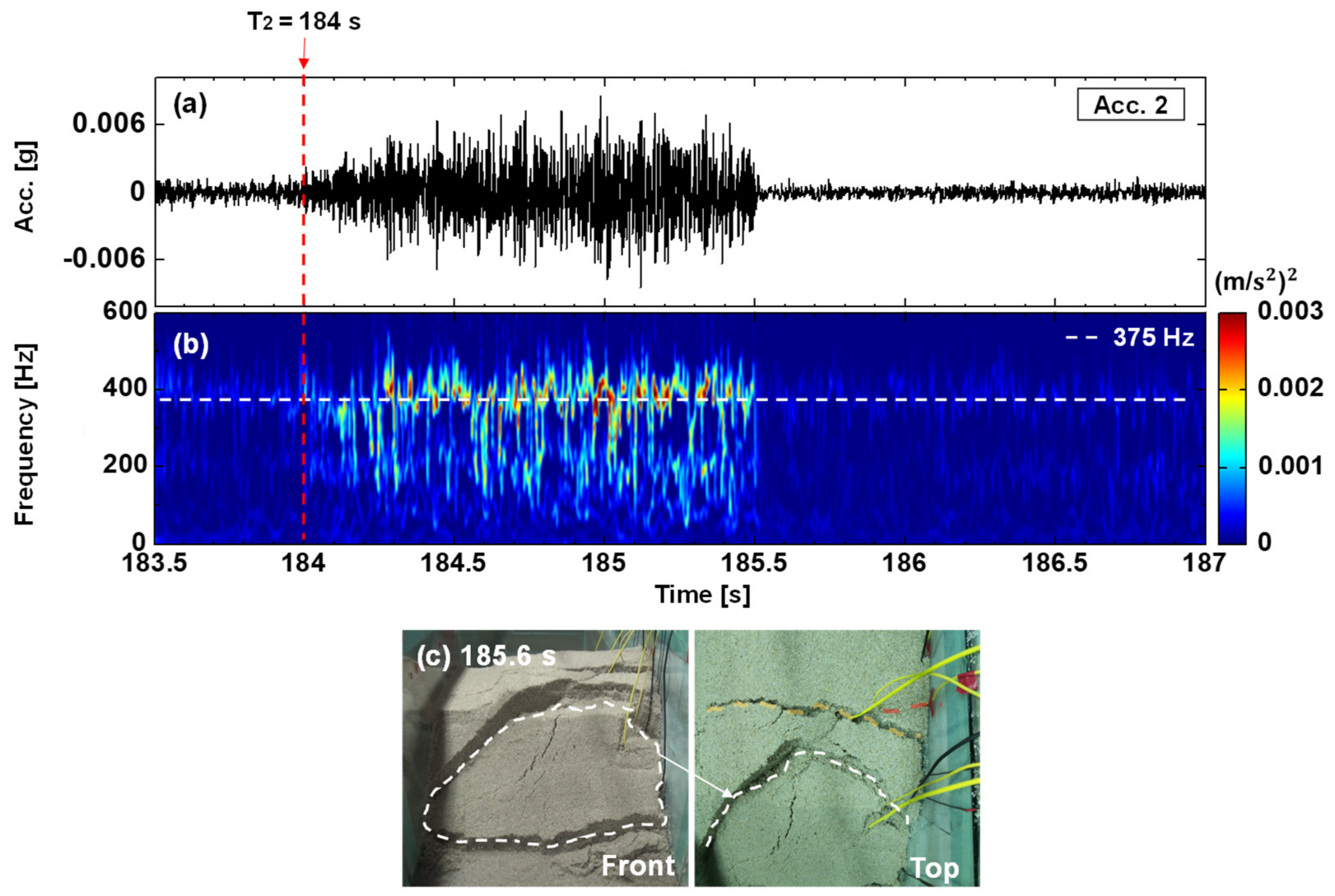
A single slide—Event 3: A single slide is defined as a rapid one-time sliding that displaces a large volume of mass [54]. Strong seismic energy is often released. Event 3 was a single slide that occurred immediately after the precursor Events 1 and 2 during 184 s (T2) to 185.6 s. The seismic signal, time–frequency spectrum, and the front and top view of Event 3 are shown in Figure 8. The amplitudes and spectral traces were larger and stronger than other events in this test due to a larger displaced mass and displacement. The duration of Event 3 was also longer than other events. It is noted that the average frequency of the seismic signal of Event 3 was 375 Hz.
(2)
An intermittent slide—Event 4: An intermittent slide is defined as the same mass sliding down multiple times on the same rupture surface [54]. An intermittent slide usually generates nearly periodic seismic signals. Event 4, an intermittent slide, occurred during 189 s (T3) ~ 207 s, which was about 3 s after Event 3. The displaced mass of the first two movements was the same mass in Event 3 and moved short distances on the same rupture surface, while another deeper rupture surface developed and part of the displaced mass of the third–fifth movements slid on it (see Supplementary Materials Video S3 for Event 4). The corresponding seismic signal, spectrum, and images of Event 4 are presented in Figure 9. For every 2–5 s there was a movement in this event. The nearly periodic seismic signals and spectral traces can easily be identified.
(3)
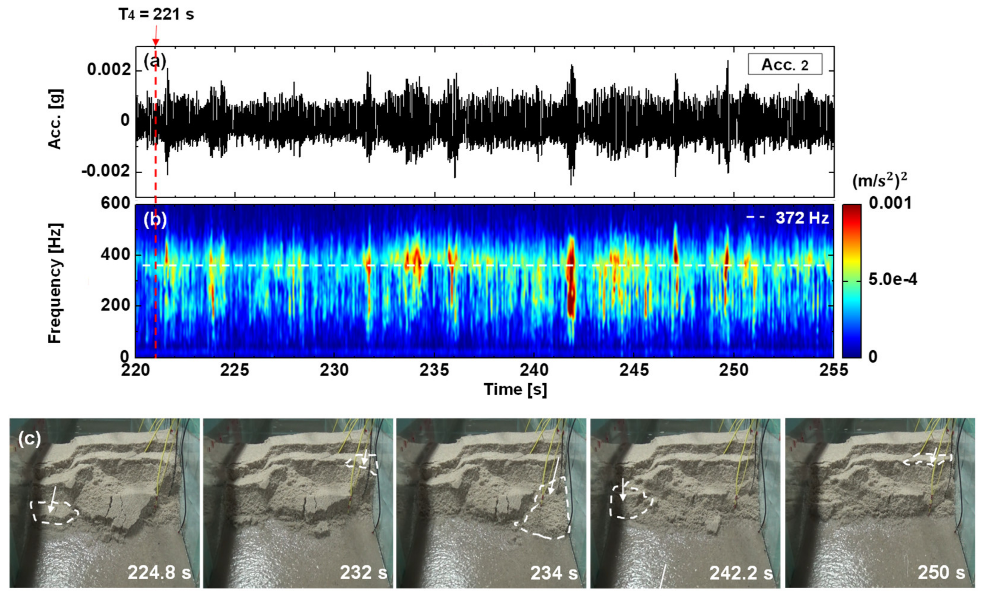
A successive slide—Event 5: A successive slide is defined as the many irregularly and randomly occurrences of sliding on multiple rupture surfaces and the displaced masses are from many different locations [54]. A successive slide usually generates aperiodic or random seismic signals. Event 5, a successive slide, occurred during 221 s (T4) ~ 251 s. In Figure 10, the signal shown was induced by random sliding of many different masses from place to place. The seismic signal was much more irregular without a pattern and the intervals between slides were random.
(4)
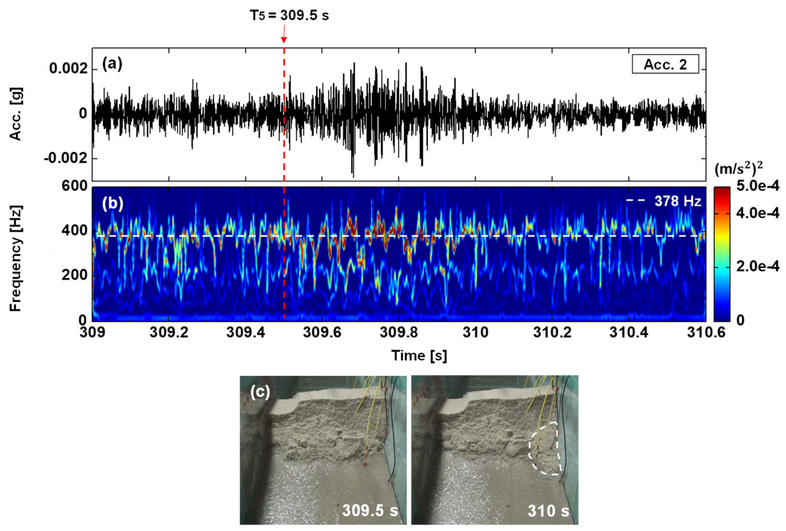
A fall—Event 6: A fall is that mass falls down through the air and falls almost vertically. Figure 11 shows the fall, Event 6, which occurred at 309.5 s (T5). The duration of Event 6 was short. The amplitudes of the signal were small and the energy traces in the spectrum were also weak owing to the fact that only a small mass fell in Event 6.
The movement types of single, intermittent, and successive slides identified in this study also occurred in the riverbank erosion tests performed by Feng et al. (2020b) [32] and the landslide tests by Feng and Chen (2021) [54]. Their failure types and failure mechanism are consistent with the results found in this study. Besides these three types of movement, we presented the fourth type, fall, which should also be helpful when correlating seismic signals to landslide events. All four types of movements are very common in retrogressive erosion due to seepage out of a dam and can be easily and correspondingly identified from induced seismic signals.
Figure 8. Event 3, the single slide: (a) seismic signal, (b) time–frequency spectrum, (c) front and top view of the single slide.
Water 13 02757 g008
Figure 9. Event 4, the intermittent slide: (a) seismic signal, (b) time–frequency spectrum, (c) series of front views the intermittent slide.
Water 13 02757 g009
Figure 10. Event 5, the successive slide: (a) seismic signal, (b) time–frequency spectrum, (c) series of front views of the successive slide.
Water 13 02757 g010
Figure 11. Event 6—the fall (a) seismic signal, (b) time–frequency spectrum, (c) front view images of the fall.
Water 13 02757 g011

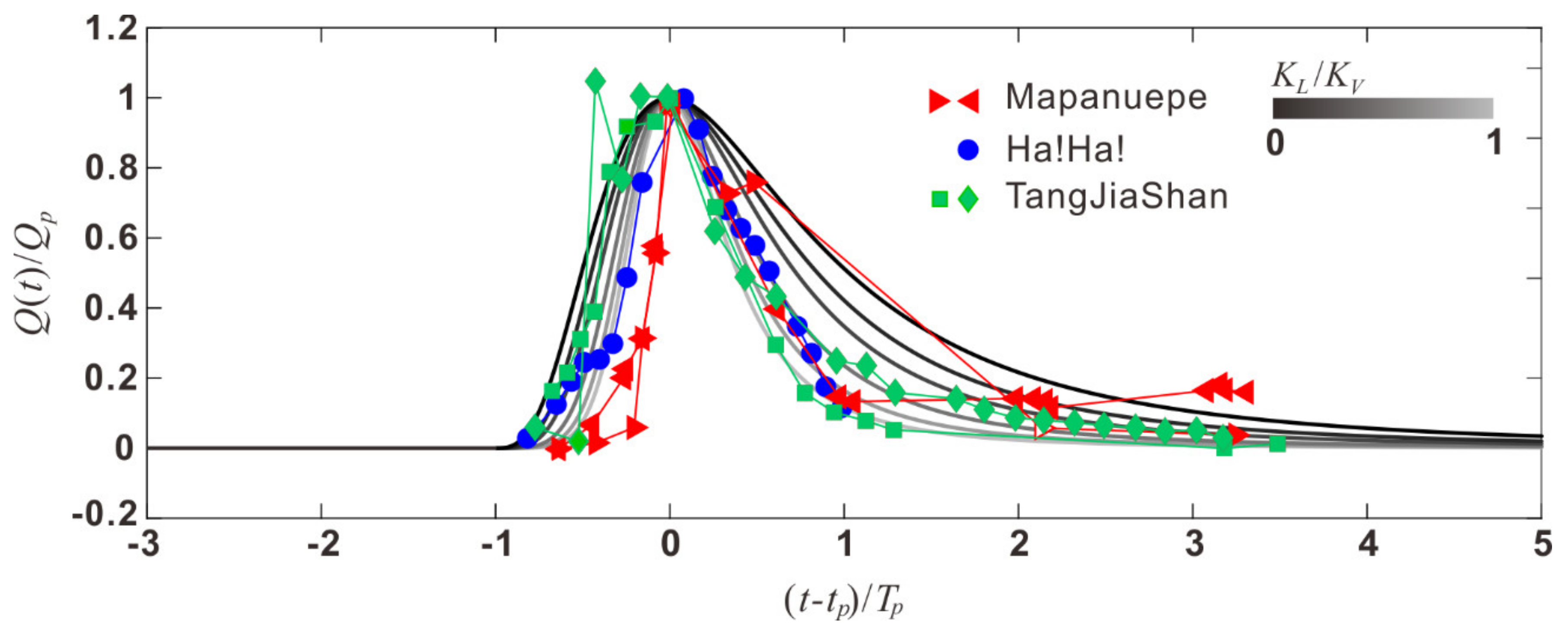
3.3. Comparison of the Dam Breach Model Result with the Breach Events from Literature

The model-predicted discharge was first verified with field measurements from literature and the test results. We reviewed four field dam breach cases: (1) Tangjiashan landslide dam breach in China [55], (2) Lake Ha! Ha! breakout flood in Canada [56], and (3) two lahar dam breaches from Mapanuepe Lake in the Philippines [57]. The essential information is shown in Table 3.
To compare the model-predicted results with the field measurements, it is convenient to present the data in dimensionless form. Since it is difficult to identify the point in time when the overtopping reached peak discharge ( T P ) from the field, we adopted the approximate equation from Capart (2013) [38] as Equation (8):
T P = 3 A L g b 2 Q P 1 / 3
where Q P is the field observed peak discharge, A L is the dammed lake area, and b is the breach channel width. The dimensionless hydrographs recorded are shown in Figure 12. The hydrographs from these different field measurements are reasonably close.
For the breach model, there are three critical parameters to control the shape and the magnitude of the hydrograph: λ , K V , and K L . To eliminate the complexity of the model, we used dimensionless hydrographs to compare with that of the test result. In that case, the hydrograph is only controlled by the ratio between the coefficients of lateral erosion ( K L ) and the vertical erosion K V . We varied the ratio ( K L / K V ) between 0 and 1. When the ratio was zero, only vertical erosion was considered. When equal erodibility in lateral and vertical directions is considered equal, i.e., their ratio is 1 (unity). The model-predicted results are shown in Figure 12 with different grayscale lines for the different coefficient ratios of erosion K L / K V . The field observation cases of Table 3 are plotted with lines and symbols for comparison. Two hydrographs are shown for the Tangjiashan event based on the data shown by Liu et al. (2010) [55], in which they used two approaches to estimate the hydrographs. The hydrography estimated from the test is represented by the blue solid curve.
In Figure 12, the predicted hydrograph becomes narrower when the ratio of K L / K V is gradually increased. The narrower curve represents the stronger lateral erosion strength. By comparing the field measurement data, most of the hydrographs showed agreement with the model prediction when the K L / K V ratio ranged from 0.5 to 1. Therefore, we can say that the lateral erosion of the dam should be considered in modeling; the lateral expansion could affect the shape of the hydrograph.
Figure 12. Dimensionless discharge hydrographs of the field-observation cases (the lines with symbols) and model-predicted hydrographs with different coefficient ratio of K L / K V (grayscale lines).
Water 13 02757 g012

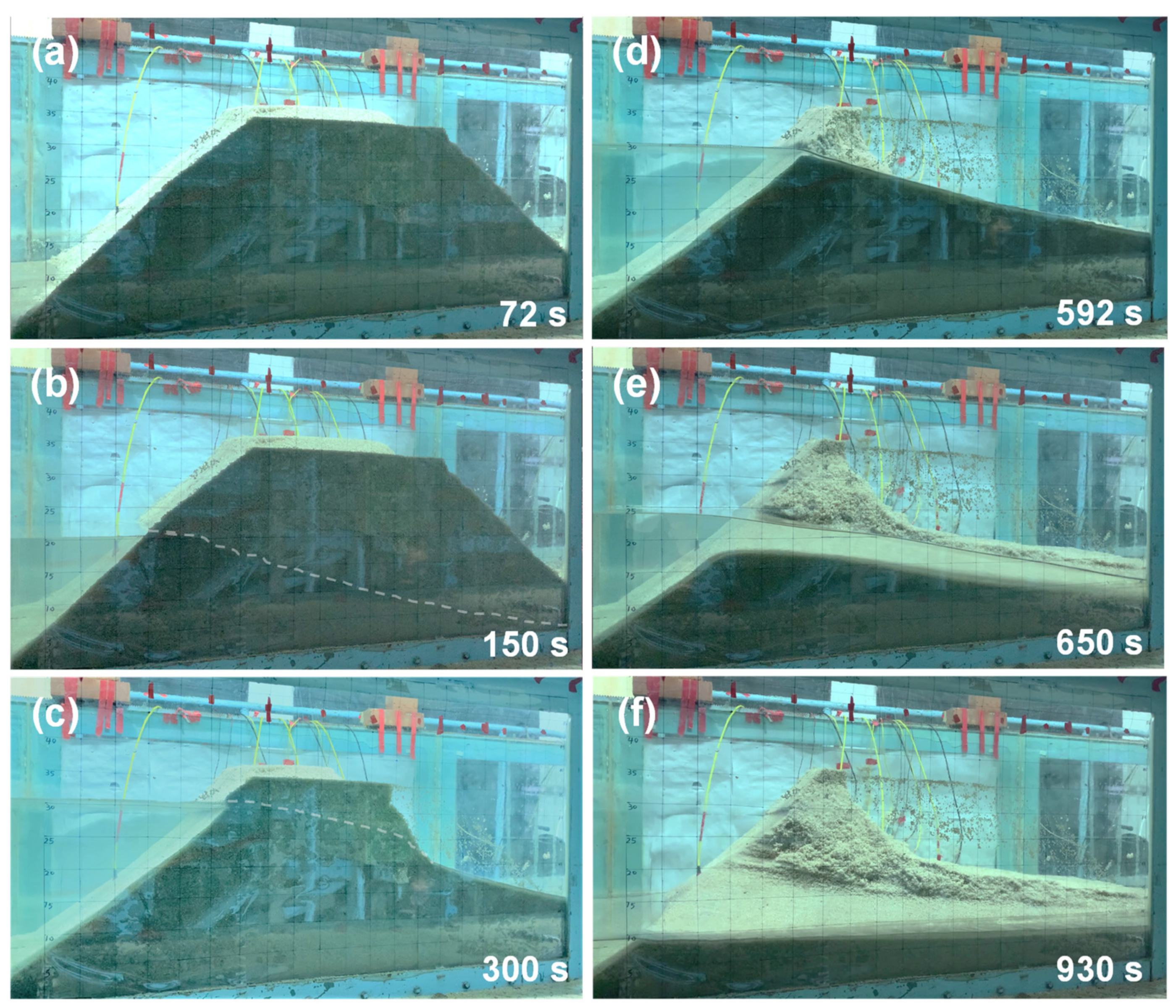
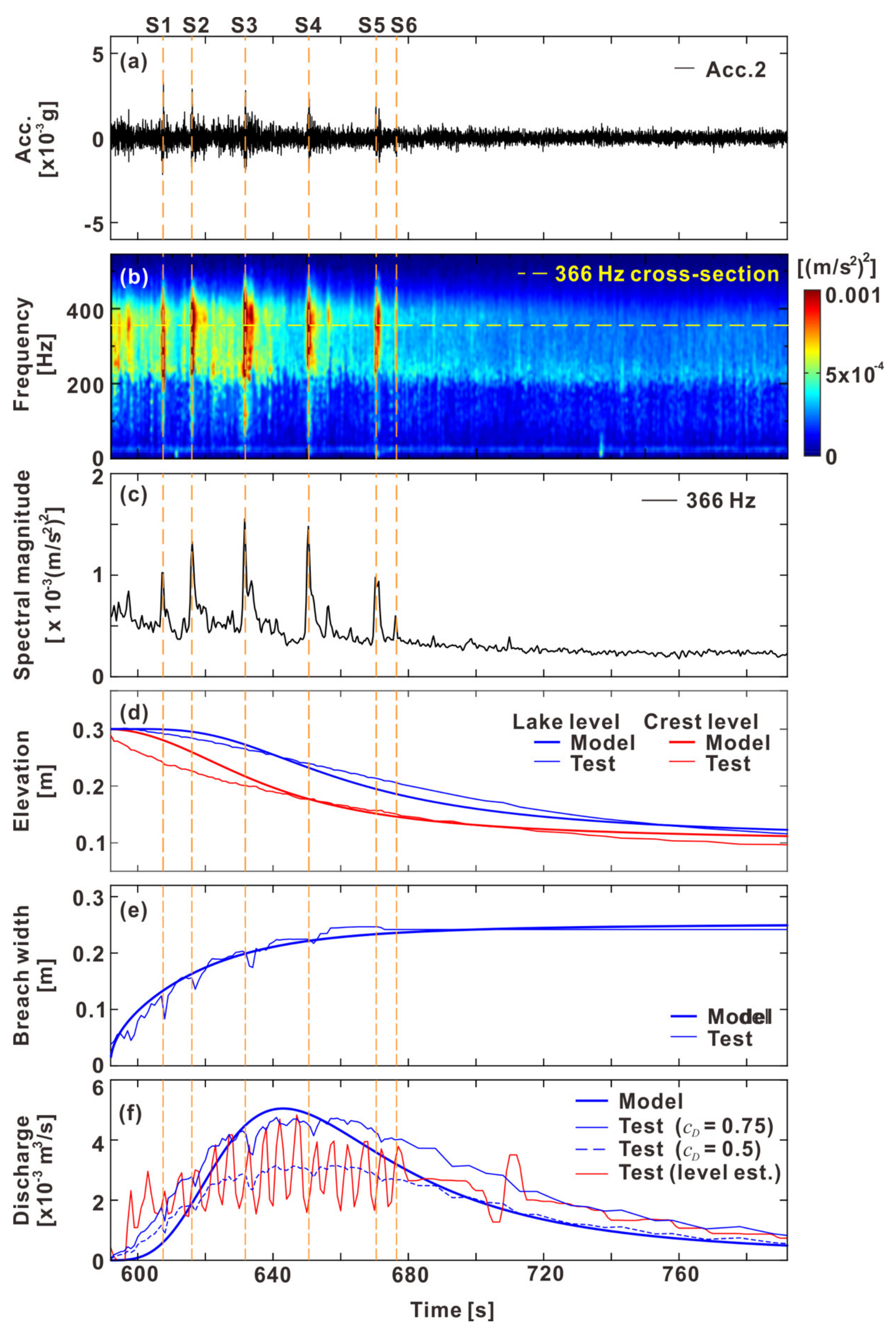
3.4. Comparision of the Dam Breach Model Result with the Test Result after Overtopping (Event 7)

To further verify the performance of the proposed dam breach model, the model result was compared with the test results. Table 4 lists the parameters used in the breach model to simulate the breach morphology of the test. To calibrate the coefficients in the model, we simply assigned the initial values of the channel width, tank level, and crest height, and then used the model to compute the values in the final stage. According to the differences between the model predictions and the test measurements, we adjusted the coefficients that showed the minimum difference. Although the calibration of the coefficients is simple in this study, the predictability of the model on breach evolution is still satisfactory.
The modeled result is presented in Figure 13 alongside Event 7 of the test result. The videos of Event 7 can be seen in Supplementary Materials Videos S6 and S7. Figure 13a,b displays the seismic signal and its time–frequency spectrum, respectively, after the overtopping (T6 = 592 s) for the test result. Figure 13c shows the spectral magnitude cross-sectional profile of 366 Hz from the spectrum in Figure 13b. The dominant seismic frequency of the signals during 592~930 s was 366 Hz. There were six noticeable amplitude and magnitude peaks, and they are marked by S1–S6 at 607, 616, 632, 651, 670, and 677 s in Figure 13a–c. They were induced by the six lateral slides of the dam during the breach. Note that the magnitude peaks in Figure 13c are more easily identified than the amplitude peaks in Figure 13a,b when corresponded to the six slides. Figure 14 shows the before-and-after photos of the six lateral slides of the dam.
In the early stages of the breach before 651 s, we can observe that the magnitudes of the lateral slides S1 to S4 gradually increased (Figure 13c) with increasing discharge. This indicates that the magnitudes of these lateral slides of the dam became increasingly larger (Figure 14a–d). As a result, vertical downcutting of the breach was more significant than lateral erosion in the early stage of the test such that the toe of the dam in the lateral direction was lowered and induced the subsequent larger lateral slides.
Figure 13d shows changes in lake level z L t and crest level z C   t . Figure 13e shows the variation of the width of the breach b t . From the test results in Figure 13d,e, we know that the tank level did not greatly decrease until 630 s, and the lowering of the tank level became prominent after 630 s. However, the lowering rate of the crest level and widening rate of the width were relatively high before 630 s, indicating that vertical downcutting and lateral erosion were quite strong.
The materials of the lateral slides (S1–S6) of the dam had an influence on the width of the breach. The width of the breach was reduced by 4.1, 2, 2.9, 0.8, 0.45, and 0.1 cm, correspondingly. When the slides occurred, the sliding materials partially blocked the breach, causing a reduction in the width of the beach. The breach was gradually opened wider again while the slid materials were taken by the overtopping flow downstream. Based on the test result (Figure 13d,e), the width evolution gradually becomes stable after the final sliding S6 at 677 s. However, the vertical downcutting of the crest was still active and caused the crest level z C to decrease until 750 s. After 750 s, the crest level became stable.
Generally, if the volume of a lateral slide is larger, the reduction in the width of the breach should be more observable. However, as a result of the test, the reduction of the width of the breach did not necessarily become larger when the volume of the lateral slides became larger. For example, when slide S1 occurred (Figure 14a), although the volume of the slide was not large, the width of the breach was significantly reduced. This is because the overtopping flow was small at that time and the transport of the slid materials was small, resulting in more slid material accumulating in the breach. When slide S3 occurred (Figure 14c), the slid volume was large, but the width change of the breach was not obvious, due to the large discharge and because the transport of the slid materials was significant such that the accumulation of slid materials in the breach was greatly reduced. Therefore, there is no obvious correlation between the change in the width of the breach and the volume of the slid materials in the test. This is mainly because larger discharges will transport more slid materials. Therefore, it may not be accurate to use the width of the breach to estimate the overtopping discharge when many lateral slides of the dam occur. In addition, we can find that after about 645 s, the lowering rate of tank level and crest level gradually decreased. The rate of change in the width of the breach from 651 to 677 s gradually decreased. Additionally, as the volume of the lateral slides gradually decreased, the influence on the width of the breach was also less; e.g., slide S5 caused marginal changes in breach width. After slide S6, the width of the breach was stable and no longer changed, and furthermore, sliding events no longer occurred.
We then compared the morphological evolutions of the breach between the model and test results. From Figure 13d, the lake level and the crest level results of the model and test results are in generally good agreement, with the exception of a slight difference at the early stage before 645 s. The difference is due to the test starting from retrogressive erosion due to seepage and then overtopping. The test dam’s strength was weaker than that of the breach model. In other words, many parts of the materials of the test dam model were formed from the very loose slid materials of the retrogressive slides. This situation is not considered in the model. In the model, we only considered the overtopping process. Therefore, the downcutting erosion rate in the test was higher during the early stage than those set in the model.
In Figure 13e, the evolution of the breach channel width of the model results shows a smoothly increasing curve. In contrast, from the test result, the evolution of the breach width was not smooth and the breach width was reduced when the four lateral slides S1–S4 occurred. These discrepancies were caused by the masses of lateral sliding materials not being considered in the model; i.e., the lateral sediment influx was not considered in the model equations. However, the model result fits the trends of the test result qualitatively well with the exception of the breach width reduction kinks in the curves. Additionally, the small pulses from the lateral slides did not affect the continuous evolution of the crest and the tank level. Therefore, to estimate the dam breach discharge, we could use the lateral erosion (or width expansion) to represent the lateral slides, especially for the loose materials.
In this study, due to the complexity of the test measurement, we did not measure the discharge directly but estimated the discharge during the breach by two different approaches. In the first approach, we considered the mass balance in the lake and assumed the lake area was maintained at a constant size during the breach and thus the discharge can be simply estimated using Equation (16) by differentiating the lake level with respect to time and multiplying by the lake area.
Q T e s t t = A L d z L t d t
The estimated discharge hydrograph of the test is shown with the thin red curve in Figure 13f. The curve is obviously zigzag in shape. This is because the discharge is estimated by the differential of the lake level. Small changes in the tank level cause large changes in the discharge; for example, the significant change in the hydrograph during t = 700~716 s, as shown in Figure 13f.
Therefore, we developed the second approach to estimate the discharge hydrograph for the test. Similar to the model derivation in Section 3, we applied the broad-crested-weir discharge equation again to estimate the discharge hydrograph of the test using Equation (17):
Q T e s t t = c D 8 g 27 b t η t 3 / 2
where c D is a discharge coefficient to be determined. In previous research, Pařílková et al. (2012) [58] and Imanian et al. (2021) [59] both pointed out the choice of c D could be highly affected by the roughness of the crest and different hydraulic head ratios. However, it is difficult to measure the roughness of the crest in the dam breach experiments, and the coefficients in our dam breach tests were not comparable with those dams without breach in the literature [58,59]. To calibrate the coefficients, we considered the tank level becoming stable in the late stage of the test, and thus used the estimated hydrograph of the late stage derived from Equation (16) to calibrate c D ; c D was set as 0.75, with b t and η t from the test measurement. The resultant hydrograph is shown in Figure 13f as the thin blue curve. To discuss in further detail, we also considered the moving average of the early stage of the test and estimate c D as 0.5. The result is shown as the dashed blue curve. However, we found that the peak discharge of the hydrograph obtained by the second approach (Equation (17)) with c D = 0.75 was close to the peak discharge obtained by the first approach (Equation (16)), i.e., the thin blue curve and thin red curve in Figure 13f, respectively. In contrast, the peak discharge of the hydrograph using c D = 0.5 was smaller than that obtained by Equation (16) (dashed blue curve and thin red curve, respectively). The hydrograph estimated with a lower coefficient may underestimate the real peak discharge due to the moving averaging process. Overall, the two hydrographs are smoother and more stable than those obtained by Equation (16). To more accurately estimate the discharge, the second approach that applied the broad-crested-weir discharge equation with c D = 0.75 is preferred.
In Figure 13f, the three hydrographs estimated for the test using the two approaches show an increase in the discharge, maintain at a fairly ”stable” discharge, and then a decrease with time, which resembles a trapezoidal shape. In contrast, the modeled discharge hydrograph (thick blue line in Figure 13f) shows a higher peak discharge at about 645 s, and this curve is similar to a bell shape without a stable discharge. The rise and decline of the hydrographs match the general trends of the estimated hydrographs from the test result.
From the perspective of disaster prevention, we hope to determine the timing of the peak discharge as preparation for early warning. Therefore, it is important to know when the peak discharge of a dam breach occurs. The timing of the peak discharge of this model is at around 645 s, which approximately matches the result of the test result. The dam breach model we proposed is simple and its estimation of hydrographs, lake and crest levels, and widths of the breach are equivalent to the test results. Therefore, it has the potential to be extended and applied to dam-breach assessment and early warning in actual situations.
From the perspective of dam breach warning and hazard reduction, the timing and magnitude of peak discharge arrival are both very important factors. From the test results, we found that when the timing of peak discharge was approaching, the lateral slides occurred more frequently and the slid masses increased. If we apply this finding to the real world, the frequency of lateral slides and their magnitudes can be indicated by seismometers and cameras to give early warning on the timing of peak discharge of a dam breach. In addition, the peak discharge and hydrograph can be calculated through the proposed dam breach model with variations of the breach width and flow depth at the crest. This model shows consistency in comparison with the field observation data and test results, and the model can be a useful tool in dam breach warning and hazard reduction.
Figure 13. Test and model results of breaching: (a) seismic signal of Acc. 2, (b) time–frequency spectrum of the seismic signal of Acc. 2, (c) spectral magnitude profile of 366 Hz cross-section shown in Figure 13b, (d) lake (tank) and crest levels of the model and test results, (e) breach width (crest channel width), (f) discharge hydrographs of the test and model.
Water 13 02757 g013
Figure 14. Before-and-after photos of the six lateral slides (S1–S6) of the dam at 607, 616, 632, 651, 670, and 677 s. The red dashed lines indicate the slid areas.
Water 13 02757 g014

4. Conclusions

This study constructed test dam models in an indoor flume to examine dam failure processes with seismic signal monitoring. A simple dam breach model was proposed and used to compare the flood process of the test. We explored the seismic signals corresponding to the sliding events during retrogressive erosion due to seepage and breaching. The monitored seismic signals corresponded clearly to the sliding events. As retrogressive erosion continued, the erosion eventually reached the crest at the upstream side of the dam, and then triggering overtopping and breaching. We verified satisfactorily this simple dam breach model by using our test result together with field observations from the literature.
Precursor seismic signals generated by cracking prior to the sliding events of the dam model were detected. Further research is strongly recommended on how to extend this observation for dam safety monitoring and prewarning to the real world. Based on the characteristics of the seismic signals, we found four types of mass movements during the retrogressive erosion process, i.e., single, intermittent, and successive slides, and fall. This result is also very useful when categorizing landslide types using seismic signals.
Overtopping discharge and lateral sliding masses of the dam are also among the important factors influencing the evolution of the breach. The masses of the lateral slides will suddenly reduce the width of the breach, but the overtopping flow will transport the masses downstream, making the width of the breach wider again. Two approaches that apply the lake level data or the broad-crested-weir discharge equation were used to estimate the hydrograph for the test. The hydrographs, obtained by the approach using the broad-crested-weir discharge equation, showed smoother and more stable hydrograph curves than those obtained by the other approach using lake level data.
The proposed simple dam breach model satisfactorily simulated the hydrograph of dam breaching and successfully assessed the vertical and lateral variations of the breach. The model can be a useful tool to help explain the dam breach process and dam breach prewarning. However, in future study, the mass input from the lateral slides can be further considered in the model.

Supplementary Materials

The following are available online at https://zenodo.org/record/5220558#.YWFuphpByUm, Video S1: Event 1 and 2, Video S2: Event 3, Video S3: Event 4, Video S4: Event 5, Video S5: Event 6, Video S6: Event 7 side view, Video S7: Event 7 front view.

Author Contributions

Conceptualization, Z.-Y.F., C.-Y.H. and S.-C.C.; methodology, Z.-Y.F. and C.-Y.H.; validation, Z.-Y.F., C.-Y.H. and I.-F.T.; formal analysis, Z.-Y.F. and C.-Y.H.; investigation, Z.-Y.F., C.-Y.H. and I.-F.T.; resources, S.-C.C.; data curation, C.-Y.H. and I.-F.T.; writing—original draft preparation, Z.-Y.F. and C.-Y.H.; writing—review and editing, Z.-Y.F., C.-Y.H., I.-F.T. and S.-C.C.; visualization, C.-Y.H. and I.-F.T. All authors have read and agreed to the published version of the manuscript.

Funding

This research was funded by Ministry of Science and Technology, Taiwan, R.O.C., grant number 109-2625-M-005-009-MY2.

Institutional Review Board Statement

Not applicable.

Informed Consent Statement

Not applicable.

Data Availability Statement

The data presented in this study are available on request from the corresponding author.

Acknowledgments

The authors acknowledge Hallam Atherton for reviewing the manuscript style.

Conflicts of Interest

The authors declare no conflict of interest.

List of symbols

z elevation of the breach channel ( m )
x streamwise direction ( m )
b breach channel width ( m )
b 0 initial breach channel width ( m )
t time (s)
J sediment flux ( m 3 / s )
z L water level (elevation) of the lake ( m )
z D dam initial elevation (before overtopping) ( m )
z C dam breach crest elevation ( m )
x C streamwise position of dam breach crest ( m )
A L lake area ( m 2 )
V E erosion volume of breach crest ( m 3 )
δ drop of the dam elevation to the breach crest elevation: z D z C   ( m )
η flow depth of the breach crest: z L z C   ( m )
S D downstream slope of the dam (initial) (-)
R D upstream slope of the dam (initial) (-)
K dimensionless sediment transport coefficient (-)
S breach channel local gradient (-)
K T scaled dimensionless sediment transport coefficient (-)
K V scaled dimensionless sediment transport coefficient in vertical direction (-)
K L scaled dimensionless sediment transport coefficient in lateral direction (-)
Q local discharge ( m 3 / s )
Q p peak discharge ( m 3 / s )
Q Test estimated test discharge ( m 3 / s )
c D dimensionless discharge coefficient (-)
τ defined operation time (accumulated discharge) ( m 2 )
λ s dimensionless scaling constant, related to the shape of the dam (-)

References

  1. Costa, J.E.; Schuster, R.L. The formation and failure of natural dams. Geol. Soc. Am. Bull. 1988, 100, 1054–1068. [Google Scholar] [CrossRef]
  2. Fan, X.M.; Dufresne, A.; Subramanian, S.S.; Strom, A.; Hermanns, R.; Stefanelli, C.T.; Hewitt, K.; Yunus, A.P.; Dunning, S.; Capra, L.; et al. The formation and impact of landslide dams—State of the art. Earth Sci. Rev. 2020, 203, 103116. [Google Scholar] [CrossRef]
  3. Chen, S.-C.; Hsu, C.-L.; Wu, T.; Chou, H.-T.; Cui, P. Landslide dams induced by typhoon Morakot and risk assessment. In Proceedings of the 5th International Conference on Debris-Flow Hazards Mitigation: Mechanics, Prediction and Assessment, Padua, Italy, 14–17 June 2011; pp. 653–660. [Google Scholar]
  4. Tsou, C.-Y.; Feng, Z.-Y.; Chigira, M. Catastrophic landslide induced by typhoon Morakot, Shiaolin, Taiwan. Geomorphology 2011, 127, 166–178. [Google Scholar] [CrossRef] [Green Version]
  5. Wu, C.-H.; Chen, S.-C.; Feng, Z.-Y. Formation, failure, and consequences of the Xiaolin landslide dam, triggered by extreme rainfall from Typhoon Morakot. Taiwan. Landslides 2014, 11, 357–367. [Google Scholar] [CrossRef] [Green Version]
  6. Feng, Z.-Y. The seismic signatures of the surge wave from the 2009 Xiaolin landslide—Dam breach in Taiwan. Hydrol. Process. 2011, 26, 1342–1351. [Google Scholar] [CrossRef]
  7. Chen, R.-F.; Chang, K.-J.; Angelier, J.; Chan, Y.-C.; Deffontaines, B.; Lee, C.-T.; Lin, M.-L. Topographical changes revealed by high-resolution airborne LiDAR data: The 1999 Tsaoling landslide induced by the Chi–Chi earthquake. Eng. Geol. 2006, 88, 160–172. [Google Scholar] [CrossRef]
  8. Chigira, M.; Wang, W.-N.; Furuya, T.; Kamai, T. Geological causes and geomorphological precursors of the Tsaoling landslide triggered by the 1999 Chi-Chi earthquake, Taiwan. Eng. Geol. 2003, 68, 259–273. [Google Scholar] [CrossRef]
  9. Li, M.-H.; Hsu, M.-H.; Hsieh, L.-S.; Teng, W.-H. Inundation Potentials Analysis for Tsao-Ling Landslide Lake Formed by Chi-Chi Earthquake in Taiwan. Nat. Hazards 2002, 25, 289–303. [Google Scholar] [CrossRef]
  10. Hsu, Y.-S.; Hsu, Y.-H. Impact of earthquake-induced dammed lakes on channel evolution and bed mobility: Case study of the Tsaoling landslide dammed lake. J. Hydrol. 2009, 374, 43–55. [Google Scholar] [CrossRef]
  11. Cui, P.; Zhou, G.G.D.; Zhu, X.H.; Zhang, J.Q. Scale amplification of natural debris flows caused by cascading landslide dam failures. Geomorphology 2013, 182, 173–189. [Google Scholar] [CrossRef]
  12. Zhou, G.G.D.; Cui, P.; Zhu, X.; Tang, J.; Chen, H.; Sun, Q. A preliminary study of the failure mechanisms of cascading landslide dams. Int. J. Sediment Res. 2015, 30, 223–234. [Google Scholar] [CrossRef]
  13. Cai, W.; Zhu, X.; Peng, A.; Wang, X.; Fan, Z. Flood Risk Analysis for Cascade Dam Systems: A Case Study in the Dadu River Basin in China. Water 2019, 11, 1365. [Google Scholar] [CrossRef] [Green Version]
  14. Říha, J.; Kotaška, S.; Petrula, L. Dam Break Modeling in a Cascade of Small Earthen Dams: Case Study of the Čižina River in the Czech Republic. Water 2020, 12, 2309. [Google Scholar] [CrossRef]
  15. Shrestha, B.B.; Nakagawa, H. Hazard assessment of the formation and failure of the Sunkoshi landslide dam in Nepal. Nat. Hazards 2016, 82, 2029–2049. [Google Scholar] [CrossRef]
  16. Suriñach, E.; Vilajosana, I.; Khazaradze, G.; Biescas, B.; Furdada, G.; Vilaplana, J.M. Seismic detection and characterization of landslides and other mass movements. Nat. Hazards Earth Syst. Sci. 2005, 5, 791–798. [Google Scholar] [CrossRef] [Green Version]
  17. Suwa, H.; Mizuno, T.; Ishii, T. Prediction of a landslide and analysis of slide motion with reference to the 2004 Ohto slide in Nara, Japan. Geomorphology 2010, 124, 157–163. [Google Scholar] [CrossRef]
  18. Yamada, M.; Matsushi, Y.; Chigira, M.; Mori, J. Seismic recordings of landslides caused by Typhoon Talas (2011), Japan. Geophys. Res. Lett. 2012, 39, 13301. [Google Scholar] [CrossRef] [Green Version]
  19. Provost, F.; Malet, J.-P.; Hibert, C.; Helmstetter, A.; Radiguet, M.; Amitrano, D.; Langet, N.; Larose, E.; Abancó, C.; Hürlimann, M.; et al. Towards a standard typology of endogenous landslide seismic sources. Earth Surf. Dyn. 2018, 6, 1059–1088. [Google Scholar] [CrossRef] [Green Version]
  20. Yan, Y.; Cui, Y.F.; Liu, D.Z.; Tang, H.; Li, Y.J.; Tian, X.; Zhang, L.; Hu, S. Seismic signal characteristics and interpretation of the 2020 “6.17” Danba landslide dam failure hazard chain process. Landslides 2021, 18, 1–18. [Google Scholar] [CrossRef]
  21. Yan, Y.; Cui, Y.; Guo, J.; Hu, S.; Wang, Z.; Yin, S. Landslide reconstruction using seismic signal characteristics and numerical simulations: Case study of the 2017 “6.24” Xinmo landslide. Eng. Geol. 2020, 270, 105582. [Google Scholar] [CrossRef]
  22. Feng, Z.-Y.; Lo, C.-M.; Lin, Q.-F. The characteristics of the seismic signals induced by landslides using a coupling of discrete element and finite difference methods. Landslides 2017, 14, 661–674. [Google Scholar] [CrossRef]
  23. Yan, Y.; Cui, P.; Chen, S.-C.; Chen, X.-Q.; Chen, H.-Y.; Chien, Y.-L. Characteristics and interpretation of the seismic signal of a field-scale landslide dam failure experiment. J. Mt. Sci. 2017, 14, 219–236. [Google Scholar] [CrossRef]
  24. Feng, Z.-Y.; Huang, H.-Y.; Chen, S.-C. Analysis of the characteristics of seismic and acoustic signals produced by a dam failure and slope erosion test. Landslides 2020, 17, 1605–1618. [Google Scholar] [CrossRef]
  25. Jiang, X.G.; Wei, Y.W.; Wu, L.; Lei, Y. Experimental investigation of failure modes and breaching characteristics of natural dams. Geomat. Nat. Hazards Risk 2018, 9, 33–48. [Google Scholar] [CrossRef]
  26. Jiang, X.; Huang, J.; Wei, Y.; Niu, Z.; Chen, F.; Zou, Z.; Zhu, Z. The influence of materials on the breaching process of natural dams. Landslides 2018, 15, 243–255. [Google Scholar]
  27. Nian, T.-K.; Wu, H.; Li, D.-Y.; Zhao, W.; Takara, K.; Zheng, D.-F. Experimental investigation on the formation process of landslide dams and a criterion of river blockage. Landslides 2020, 17, 2547–2562. [Google Scholar] [CrossRef]
  28. Zhu, X.; Liu, B.; Peng, J.; Zhang, Z.; Zhuang, J.; Huang, W.; Leng, Y.; Duan, Z. Experimental study on the longitudinal evolution of the overtopping breaching of noncohesive landslide dams. Eng. Geol. 2021, 288, 106137. [Google Scholar] [CrossRef]
  29. Hu, W.; Scaringi, G.; Xu, Q.; Huang, R.Q. Acoustic Emissions and Microseismicity in Granular Slopes Prior to Failure and Flow-Like Motion: The Potential for Early Warning. Geophys. Res. Lett. 2018, 45, 10406–10415. [Google Scholar] [CrossRef]
  30. Poli, P. Creep and slip: Seismic precursors to the Nuugaatsiaq landslide (Greenland). Geophys. Res. Lett. 2017, 44, 8832–8836. [Google Scholar] [CrossRef]
  31. Butler, R. Seismic precursors to a 2017 Nuugaatsiaq, Greenland, earthquake–landslide–tsunami event. Nat. Hazards 2019, 96, 961–973. [Google Scholar] [CrossRef]
  32. Feng, Z.-Y.; Hsu, C.-M.; Chen, S.-H. Discussion on the Characteristics of Seismic Signals Due to Riverbank Landslides from Laboratory Tests. Water 2019, 12, 83. [Google Scholar] [CrossRef] [Green Version]
  33. Huang, N.E.; Shen, Z.; Long, S.R.; Wu, M.L.C.; Shih, H.H.; Zheng, Q.N.; Yen, N.C.; Tung, C.C.; Liu, H.H. The empirical mode decomposition and the Hilbert spectrum for nonlinear and non-stationary time series analysis. Proc. R. Soc. A Math. Phys. Eng. Sci. 1998, 454, 903–995. [Google Scholar] [CrossRef]
  34. Takayama, S.; Miyata, S.; Fujimoto, M.; Satofuka, Y. Numerical simulation method for predicting a flood hydrograph due to progressive failure of a landslide dam. Landslides 2021. [Google Scholar] [CrossRef]
  35. Wu, W. Simplified physically based model of earthen embankment breaching. J. Hydraul. Eng. 2011, 137, 1549–1564. [Google Scholar] [CrossRef]
  36. Alhasan, Z.; Jandora, J.; Říha, J. Study of dam-break due to overtopping of four small dams in the Czech Republic. Acta Univ. Agric. Silvic. Mendel. Brun. 2015, 63, 717–729. [Google Scholar] [CrossRef] [Green Version]
  37. Tian, S.; Dai, X.; Wang, G.; Lu, Y.; Chen, J. Formation and evolution characteristics of dam breach and tailings flow from dam failure: An experimental study. Nat. Hazards 2021, 107, 1–18. [Google Scholar] [CrossRef]
  38. Capart, H. Analytical solutions for gradual dam breaching and downstream river flooding. Water Resour. Res. 2013, 49, 1968–1987. [Google Scholar] [CrossRef]
  39. Capart, H.; Hsu, J.P.C.; Lai, S.Y.J.; Hsieh, M.-L. Formation and decay of a tributary-dammed lake, Laonong River, Taiwan. Water Resour. Res. 2010, 46, W11522. [Google Scholar] [CrossRef] [Green Version]
  40. Lane, E.W. The importance of fluvial morphology in hydraulic engineering. Proc. Am. Soc. Civ. Eng. 1955, 81, 1–17. [Google Scholar]
  41. Alhasan, Z.; Jandora, J.; Říha, J. Comparison of specific sediment transport rates obtained from empirical formulae and dam breaching experiments. Environ. Fluid Mech. 2016, 16, 997–1019. [Google Scholar] [CrossRef]
  42. AnCAD, Inc. Visual Signal Reference Guide, Version1.6. Available online: http://www.ancad.com.tw/VisualSignal/doc/1.6/RefGuide.html (accessed on 15 July 2021). (In Chinese).
  43. Paola, C.; Voller, V.R. A generalized Exner equation for sediment mass balance. J. Geophys. Res. Earth Surf. 2005, 110, F04014. [Google Scholar] [CrossRef]
  44. Visser, P.J. Application of sediment transport formulae to sand-dike breach erosion. Oceanogr. Lit. Rev. 1996, 43, 954. [Google Scholar]
  45. Haddadchi, A.; Omid, M.H.; Dehghani, A.A. Bedload equation analysis using bed load-material grain size. J. Hydrol. Hydromech. 2013, 61, 241–249. [Google Scholar] [CrossRef] [Green Version]
  46. Cao, Z.; Yue, Z.; Pender, G. Landslide dam failure and flood hydraulics. Part II: Coupled mathematical modelling. Nat. Hazards 2011, 59, 1021–1045. [Google Scholar] [CrossRef]
  47. Capart, H.; Bellal, M.; Young, D.-L. Self-similar evolution of semi-infinite alluvial channels with moving boundaries. J. Sediment. Res. 2007, 77, 13–22. [Google Scholar] [CrossRef]
  48. Hsu, J.P.C.; Capart, H. Onset and growth of tributary-dammed lakes. Water Resour. Res. 2008, 44, W11201. [Google Scholar] [CrossRef] [Green Version]
  49. Voller, V.R.; Swenson, J.B.; Paola, C. An analytical solution for a Stefan problem with variable latent heat. Int. J. Heat Mass Transf. 2004, 47, 5387–5390. [Google Scholar] [CrossRef]
  50. Lai, S.Y.J.; Capart, H. Two-diffusion description of hyperpycnal deltas. J. Geophys. Res. Space Phys. 2007, 112, F03005. [Google Scholar] [CrossRef] [Green Version]
  51. Lai, S.Y.J.; Capart, H. Reservoir infill by hyperpycnal deltas over bedrock. Geophys. Res. Lett. 2009, 36, L08402. [Google Scholar] [CrossRef]
  52. Carslaw, H.S.; Jaeger, J.C. Conduction of Heat in Solids; Oxford University Press: Oxford, UK, 1959. [Google Scholar]
  53. Henderson, F.M. Open Channel Flow; Macmillan: New York, NY, USA, 1966. [Google Scholar]
  54. Feng, Z.-Y.; Chen, S.-H. Discussions on landslide types and seismic signals produced by the soil rupture due to seepage and retrogressive erosion. Landslides 2021, 18, 2265–2279. [Google Scholar] [CrossRef]
  55. Liu, N.; Chen, Z.; Zhang, J.; Lin, W.; Chen, W.; Xu, W. Draining the Tangjiashan barrier lake. J. Hydraul. Eng. 2010, 136, 914–923. [Google Scholar] [CrossRef]
  56. Capart, H.; Spinewine, B.; Young, D.; Zech, Y.; Brooks, G.R.; Leclerc, M.; Secretan, Y. The 1996 Lake Ha! Ha! breakout flood, Québec: Test data for geomorphic flood routing methods. J. Hydraul. Res. 2007, 45 (Suppl. 1), 97–109. [Google Scholar] [CrossRef]
  57. Umbal, J.V.; Rodolfo, K.S. The 1991 Lahars of Southwestern Mount Pinatubo and Evolution of the Lahar-Dammed Mapanuepe Lake. In Fire and Mud: Eruptions and Lahars of Mount Pinatubo, Philippines; Newhall, C.G., Punongbayan, R.S., Eds.; University of Washington Press: Washington, DC, USA, 1996; pp. 951–970. [Google Scholar]
  58. Pařílková, J.; Říha, J.; Zachoval, Z. The influence of roughness on the discharge coefficient of a broad-crested weir. J. Hydrol. Hydromech. 2012, 60, 101–114. [Google Scholar] [CrossRef] [Green Version]
  59. Imanian, H.; Mohammadian, A.; Hoshyar, P. Experimental and numerical study of flow over a broad-crested weir under different hydraulic head ratios. Flow Meas. Instrum. 2021, 80, 102004. [Google Scholar] [CrossRef]
Figure 1. Layout of the test flume and the dam model.
Water 13 02757 g001
Figure 2. (a) The side view of the dam model and (b) front view of the dam model.
Water 13 02757 g002
Figure 3. Sensor configuration in the dam model (the numbering of the sensors is marked near each sensor).
Water 13 02757 g003
Figure 4. Schematic and parameters of the proposed dam breach model.
Water 13 02757 g004
Figure 5. Test measurements: (a) water level of the tank, (b) seismic signal of Acc. 2, (c) volumetric water content, (d) pore pressure.
Water 13 02757 g005
Figure 6. Side-view images at different test stages.
Water 13 02757 g006
Figure 7. Events 1 and 2, the precursors prior to the Event 3 slide: (a) seismic signal, (b) time–frequency spectrum, (c) top view of the Crack 1 in red dashed line and Crack 2 in orange dashed line.
Water 13 02757 g007
Table 1. The dimensions of the dam model.
Slope (°)Height (m)Crest Width
(m)
Bottom Length (m)Channel Width (m)Maximum Water Level
(m)
450.40.351.150.60.3
Table 2. Test processes and the selected important events.
Time, sEventVariation of the Seismic Signals
0–116The flow pump was opened and the sluice was opened.Frequency of the flow pump: 106 Hz, 227 Hz
76T0 = 76 s when water reached the upstream toe of the dam model; the water continued to fill the tank up to 0.3 cm.-
116The flow pump was closed; the sluice remained opened.Frequency of the environment: 101 Hz;
130A tapping was made to leave a time marker.Amplitudes of the signals at 130 s were very high.
180.6–183.5T1 =180.6 s; Event 1 and 2 precursor signals; one smaller crack and one larger crack developed prior to a slide (see Supplementary Materials Video S1)Two precursor seismic signals occurred prior to a slide; the 1st with lower energy; the 2nd with higher energy.
184–185.6T2 = 184 s; a single slide (Event 3) occurred (see Supplementary Materials Video S2)Seismic signals significantly increased
189–207T3 = 189 s; an intermittent slide (Event 4) occurred (see Supplementary Materials Video S3); retrogressive erosionSeismic signals significantly increased nearly periodically in about 2 to 5 s.
221–251T4 = 221 s; a successive slide (Event 5) occurred (see Supplementary Materials Video S4); retrogressive erosionSeismic signals significantly increased aperiodically.
309.5–310T5 = 309.5 s; a fall (or collapse) (Event 6) occurred (see Supplementary Materials Video S5)Seismic signals suddenly increased and the duration was very short.
412–510Many single slides with different magnitudes occurred; retrogressive erosionSeismic signals significantly increased with different corresponding amplitudes
592–930T6 = 592 s; Overtopping process (Event 7) (see Supplementary Materials Videos S6 and S7); the sluice was then closed; six lateral slides occurred.Seismic signals significantly increased when the six lateral slides occurred. Strong spectral traces appear around 220–420 Hz in the time–frequency spectrum due to the overtopping water flow.
930The end of the test
Table 3. Information on dam breach events from literature [38].
Dam/LakeDateAL
( 10 6   m 2 )
b
(m)
Qp
( 10 3   m 3 / s )
Source
Mapanuepe25–27 August 19916.7700.65Umbal and Rodolfo (1996) [57]
12–16 October 19916.7700.39
Ha!Ha!19–22 July 19966900.85Capart et al. (2007) [56]
Tangjiashan10–11 June 20086.41106.5Liu et al. (2010) [55]
Table 4. Parameters for the proposed dam breach model for the test dam.
Parameters/UnitValueSource
z D 0 [m]0.3Measured from the initial dimensions of the test dam
z C 0 [m]0.3
z L 0 [m]0.3
b 0 [m]0.015
A L [m2]2.22
dt [s]0.005Numerical calculation time step
K V 1.875Calibrated from the test result
K L / K V 0.1375
Publisher’s Note: MDPI stays neutral with regard to jurisdictional claims in published maps and institutional affiliations.

