Abstract
Sustainable agriculture in arid regions necessitates that the quality of groundwater be carefully monitored; otherwise, low-quality irrigation water may cause soil degradation and negatively impact crop productivity. This study aimed to evaluate the quality of groundwater samples collected from the wells in the quaternary aquifer, which are located in the Western Desert (WD) and the Central Nile Delta (CND), by integrating a multivariate analysis, proximal remote sensing data, and data-driven modeling (adaptive neuro-fuzzy inference system (ANFIS) and support vector machine regression (SVMR)). Data on the physiochemical parameters were subjected to multivariate analysis to ease the interpretation of groundwater quality. Then, six irrigation water quality indices (IWQIs) were calculated, and the original spectral reflectance (OSR) of groundwater samples were collected in the 302–1148 nm range, with the optimal spectral wavelength intervals corresponding to each of the six IWQIs determined through correlation coefficients (r). Finally, the performance of both the ANFIS and SVMR models for evaluating the IWQIs was investigated based on effective spectral reflectance bands. From the multivariate analysis, it was concluded that the combination of factor analysis and principal component analysis was found to be advantageous to examining and interpreting the behavior of groundwater quality in both regions, as well as predicting the variables that may impact groundwater quality by illuminating the relationship between physiochemical parameters and the factors or components of both analyses. The analysis of the six IWQIs revealed that the majority of groundwater samples from the CND were highly suitable for irrigation purposes, whereas most of the groundwater from the WD can be used with some limitations to avoid salinity and alkalinity issues in the long term. The high r values between the six IWQIs and OSR were located at wavelength intervals of 302–318, 358–900, and 1074–1148 nm, and the peak value of r for these was relatively flat. Finally, the ANFIS and SVMR both obtained satisfactory degrees of model accuracy for evaluating the IWQIs, but the ANFIS model (R2 = 0.74–1.0) was superior to the SVMR (R2 = 0.01–0.88) in both the training and testing series. Finally, the multivariate analysis was able to easily interpret groundwater quality and ground-based remote sensing on the basis of spectral reflectance bands via the ANFIS model, which could be used as a fast and low-cost onsite tool to estimate the IWQIs of groundwater.
1. Introduction
Groundwater is regarded as one of the most essential irrigation resources, especially in countries that face extreme water scarcity. However, various agricultural and other human activities in recent decades have resulted in the severe pollution of groundwater, making it unsuitable for irrigation purposes under ordinary conditions. Therefore, water quality, which is fundamental to groundwater management and irrigation water, should be regularly evaluated and monitored.
The viability of any water resource for irrigation purposes is evaluated through several irrigation water quality indices (IWQIs) [1]. These indices, which are based on several physiochemical variables of water, include a water quality index (WQI), residual sodium bicarbonate (RSBC), total hardness (TH), potential salinity (PS), residual sodium carbonate (RSC), magnesium hazard (MH), and others [2,3,4,5,6]. The main objective of each index is to determine groundwater’s suitability for either drinking or irrigation purposes. For example, the primary objective of the WQI is to evaluate the overall water quality levels by transforming a wide range of selected physiochemical water variables into a single numerical value using a simple mathematical function [4,7,8]. Again, this index can be considered a simplified model of the complex reality of water quality. The main objective of MH is to represent the excess of Mg2+ in irrigation water. A high MH value in irrigation water may lead to soil alkalinity, as well as reduce the infiltration capacity of soil if a large amount of water is adsorbed between magnesium and clay particles [5,9]. The primary goal of RSC is to measure the relationship between the sum of CO32− and HCO3− and that of Ca2+ and Mg2+ [10]. A high-RSC value in irrigation water makes the soil infertile because of the deposition of sodium carbonate [10,11,12]. PS is a characterization of the dominant Cl− and SO42− in irrigation water [13]. Since salts with low solubility precipitate in the soil and accumulate with each successive round of irrigation, this leads to issues of soil salinity. Thus, a high PS value would foster soil permeability problems and thus inhibit the water absorption by crops [4]. Therefore, various important dissolved ions in groundwater such as Na+, K+, Ca2+, Mg2+, Cl−, SO42−, CO32−, and HCO3− represent a common factor in determining various IWQIs. This is because the productivity of field crops as well as the different physiochemical properties of soil are mainly dependent on the concentrations of these ions in irrigation water. If the concentration of some particular ions exceeds a specific threshold, the water cannot be suitable for irrigation purposes. For example, excessive concentrations of Na+ in irrigation water reduce soil permeability as well as hinder the uptake of essential ions (Ca2+, Mg2+, and K+). Excessive concentrations of Mg2+ can lead to soil alkalinity. Excessive concentrations of HCO3− negatively affect the plant uptake and metabolism of nutrients. Finally, many of these negative impacts of excessive particular ions limit the growth and productivity of most field crops [4,5,9]
The evaluation of groundwater quality through the analysis of a large number of physiochemical parameters produces complex data matrices, which make the understanding and interpretation of the intricacies of water quality difficult. Recently, multivariate statistical methods such as factor analysis (FA) and principal component analysis (PCA) have been used to aid in the improved interpretation of large and complex data matrices relating to water quality without losing necessary information collected from actual observations [14,15,16,17]. Both types of analysis, incorporating several physiochemical parameters, are applied for extracting new important components or factors that account for most of the variations in groundwater quality [16,18,19,20]. Using both analytical methods, each new factor produces its own effect on groundwater quality within areas under investigation. In summary, FA can determine the key parameters that explain the original data to the greatest extent, whereas PCA can provide a comprehensive picture of the interrelationships between all parameters and confirm their relative degrees of influence. Thus, in the present study, FA was used together with PCA to examine the influence of different of physicochemical parameters on groundwater quality.
Although all of the IWQIs are simple indicators that reflect overall water quality levels, the establishment of these indices using conventional procedures, such as collecting samples at fixed points in the field and then analyzing several physiochemical parameters in the laboratory with intensive statistical analysis, makes the compilation of these indices a time consuming, laborious, and ineffective process for effectively monitoring and managing groundwater quality. Importantly, it is not easy to determine the temporal and spatial variations in water quality demonstrated by these indices, which play an essential role in the evaluation and management of groundwater quality for irrigation purposes [21].
To overcome the limitations of IWQIs, field-measured spectroscopy has been shown to be a practical tool for the integrative evaluation and monitoring of the temporal and spatial variations of several water quality variables on a large scale in a quick and cost-effective manner. The advantages of this tool include a large number of spectral reflectance bands and information that is significantly influenced by the changes that occur in the concentrations and types of physiochemical parameters, such as the content levels of chlorophyll, total suspended solids (TSSs), TH, total alkalinity (TA), total dissolved substances (TDS), salinity, the content of nitrogen and phosphorus, dissolved organic carbon, chemical oxygen demand (COD), and biological oxygen demand (BOD) [22,23,24,25,26,27,28,29,30]. For instance, a close relationship has been found between the total phosphorus in water and spectral reflectance wavebands in blue (450–510 nm) and green (500–600 nm) regions [31]. Gitelson et al. [32] reported that spectral reflectance from water surfaces in the range of 700–900 nm wavebands is sensitive to changes in the TSS concentration. Liu et al. [33] reported that spectral reflectance in the range of 560 to 780 nm was adequate for detecting suspended particulate matter in water. Xing et al. [28] also noted that the curve patterns of the relationship between spectral reflectance wavebands and water quality variables exhibited the maximum spectral response at intervals of 990–999 nm for NH3–N, 760–770 nm for BOD, and 460–475 nm for COD, TH, TA, and TDS. However, because the spectral reflectance measurements generate a large volume of data, the analysis of spectral reflectance data using an appropriate statistical model remains a critical step toward the discovery of the optimal relationship between spectral data and IWQIs.
Recently, new modeling frameworks, such as data-driven modeling (DDM) or data mining, have seen significantly increased use in the creation and application of computational intelligence and computer resources for water-related issues [34,35]. These methodologies constitute an approach for estimating water quality parameters obtained from field datasets and mapping the relationship between water quality variables according to spatial and temporal variability [36]. DDM is focused on the analysis of the data that characterizes the system being studied, particularly a model that can be described based on identifying links between the system’s parameters (input, internal, and output variables) without specific knowledge of the physical behavior [37]. The DDM encompasses different categories commonly categorized into statistical and artificial intelligent models that include neural networks such as fuzzy systems and evolutionary computing, as well as other artificial intelligence and machine learning fields such as support vector machine regression (SVMR) [38]. SVMR uses a kernel function to map variable inputs into a high-dimensional feature space and can therefore handle high-dimensional input vectors [39]. Thus, it can provide a more rational solution than linear methodologies [40]. The development and current progress in the integration of various artificial intelligence techniques (knowledge-based systems, genetic algorithms, artificial neural networks, and fuzzy inference systems (FISs)) in water quality modeling, sediment transportation, and dissolved oxygen concentration have been studied by several researchers [38,41,42,43].
Thus far, the prediction of IWQIs using adaptive neuro-fuzzy inference system (ANFIS) and SVMR models based on spectral reflectance bands has not been addressed. Only one study that we are aware of has focused on predicting the drinking WQI of surface water using the SVMR based on spectral reflectance indices (SRIs) [44]. Additionally, Xing et al. [28] used a partial least-squares regression (PLSR) and extreme learning machine to predict the TH in sewage water using the entire range of spectrum wavebands (350–2500 nm).
The primary objectives of this study are to (i) incorporate the different physiochemical parameters into a multivariate analysis to better understand and interpret the major contributing parameters that influence the groundwater quality of two distinct regions; (ii) evaluate the suitability of the groundwater in both regions for irrigation purposes based on various IWQIs; (iii) determine the optimal spectral wavelengths interval corresponding to different IWQIs; and (vi) evaluate the ANFIS and SVMR models based on the spectral reflectance bands to predict and simulate the IWQIs of groundwater. We not only evaluate the suitability of groundwater for irrigation purposes using multivariate analysis and a wide variety of IWQIs but also develop a new algorithm that can simulate and predict the quality of water resources by means of field-measured spectroscopy.
2. Materials and Methods
2.1. Study Area
The quaternary aquifer represents the main water-bearing formation for the two regions that make up the study area. The first of these (29°0′–29°30′ N and 30°20′–31°10′ E) is located in the El Fayoum depression in the Western Desert (WD) of Egypt and has an area of approximately 1200 km2. The second region (30°30′–30°55′ N and 30°40′–31°00′ E) is located in the Central Nile Delta (CND) and has an area of approximately half that of the first region.
The Quaternary deposits in the WD region are composed of varying grain sizes ranged from sandy clay and sometimes gravelly at the west to silt clay sediments at the east. The Quaternary aquifer in the CND region is generally composed of sand with a rich content of clay. The depth of the groundwater surface varies from few centimeters to 9.1 m and from 25 to 30 m in the WD and CND regions, respectively [29].
2.2. Sample Collection, Ionic Analysis, and Irrigation Groundwater Quality Evaluation
A total of 40 groundwater samples, 15 of which were from the first region and 25 were from the second, were collected during the summer of 2019 (Figure 1). The samples were kept at 4 °C and delivered to the laboratory on the day they were collected for physiochemical analysis. The temperature, electrical conductivity, hydrogen ion activity (pH), and total dissolved solids (TDS) were measured in situ for each sample using a portable calibrated conductivity multi-parameter instrument (Hanna HI 9033). The different ionic concentrations, which are the basis for calculating the different variables related to irrigation groundwater quality, were analyzed according to the Standard Methods for the Examination of Water and Wastewater [45]. The total concentrations of Mg2+, Ca2+, and Cl− were estimated via the titration method using the ethylenediamine tetra-acetic acid for the first two ions and silver nitrate for the last ion. The total concentrations of Na+ and K+ were estimated using a flame photometer (ELEX 6361, Eppendorf AG, Hamburg, Germany). The concentrations of HCO3− and CO32− were determined using the titrimetric method, whereas the content of SO42− was determined with an ultraviolet visible spectrophotometer (DR/2040, Loveland, CO, USA). Before the ionic analysis, all of the samples were filtered through 0.45 µm of porosity to collect the solutions containing the dissolved elements only. All of the ionic concentrations are expressed in milligrams per liter.
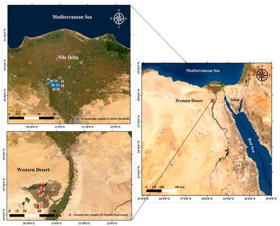
Figure 1.
Location map of the El Fayoum depression in the Western Desert (red points) and the Central Nile Delta (blue points) and their sampling points.
2.3. Evaluation of the Quality of Groundwater for Irrigation Purposes
To ascertain the suitability of groundwater for irrigation purposes, quality variables such as the WQI, RSBC, RSC, TH, PS, and MH, which cause various problems for soil–water–plant relationships, were calculated for the groundwater samples of the two regions. Table 1 lists the formula and references of these variables.

Table 1.
Formula and references for different irrigation water quality indices applied in this study.
The WQI was first proposed by Horton [47]. This index has the capacity to transform large quantities of water parameter data into a single value, which helps us intensively interpret the impacts of several water parameters on overall water quality levels [4,7]. In this capacity, the index is a significant marker for the evaluation and management of groundwater for irrigation purposes. In this study, the WQI was calculated using the following equation [48]:
The WQI was calculated in two steps. In the first step, the dominant physiochemical parameters that play a vital role in the estimation of water quality for irrigation purposes were identified, which in this study are SAR, EC, Na+, Cl−, and HCO3−. In the second step, the aggregation weights (Wi) and water quality measurement parameter value (Qi) were determined based on each physiochemical parameter value, according the criteria proposed by Ayers and Westcot [48].
The values of Qi were calculated using the following equation:
where Qmax is the maximum value of Qi for each class; Xij is the observed value of each physiochemical parameter; Xinf is the lower limit value of the class to which the parameter belongs; Qimap and Xamp respectively refer the class amplitude and class amplitude to which the parameter belongs.
Finally, the values of Wi were normalized, and their final sum equals one according to the following equation:
where Wi and F are respectively corresponding to relative weight of the physiochemical parameters for WQI and a constant value of component 1; Aij is the parameter i that can be explained by factor j; i is the number of physiochemical parameters choose in WQI and varying from 1 to n; and j is the number of factors selected in WQI and ranging from 1 to k.
According to Equation (3), the normalized weights of the SAR, EC, Na+, Cl−, and HCO3− are 0.189, 0.211, 0.204, 0.194, and 0.202, respectively.
The MH plays a pivotal role in determining the suitability of water for irrigation purposes, where the high concentrations of Mg2+, as well as Ca2+ in water, can increase the soil pH, decrease the availability of phosphorous and the soil quality, and finally, cause a significant decline in crop production [11,49]. An HM value of <50 is recommended for irrigation purposes, whereas one >50 is considered unsuitable for irrigation.
Generally, irrigation water with high salinity causes changes in soil structure and permeability, toxicity for plants, and reduced water availability. Thus, the PS is another key variable for irrigation water quality guidelines. It is defined as the Cl− concentrations plus half of the SO42− concentrations [13]. Usually, irrigation water with PS values lower than three is considered fit for irrigation purpose.
The TH of water is the result of the presence of Ca2+ and Mg2+ in it. Although both ions are essential for plant growth and certain concentrations of them in irrigation water are beneficial, very high TH values in irrigation water can reduce irrigation efficiency because of the precipitation of both ions throughout the irrigation system. Additionally, very low values of TH can induce corrosion in the system. Hence, the TH variable is also considered an indicator of irrigation water quality. Groundwater with a TH <75 mg L−1 is usually classified as soft, whereas >300 mg L−1 is considered very hard [2].
For irrigation purposes, RSC (NaCO3) and RSBC (NaHCO3) are usually used to predict the relationship of CO3 and HCO3 concentrations and those of Ca2+ and Mg2+. If the CO3 and HCO3 concentrations in the irrigation water are less than the Ca2+ and Mg2+ levels, the values of the RSC and RSBC become negative. This indicates little risk of Na+ accumulation in the soil due to offsetting the levels of Ca2+ and Mg2+; the opposite holds true for positive values.
2.4. Measurements of Spectral Reflectance
For this study, the groundwater samples were placed in black cylindrical cups with a diameter of 25 cm and a depth of 10 cm. The spectral reflectance data were collected from the water surface of each sample using the passive reflectance sensor (tec5 AG, Oberursel, Germany) with a spectral range of 302–1148 nm, a sampling interval of 2 nm, and a probe field angle of 12°. The spectral readings were collected under sunny and windless conditions, and the probe was held vertically at ≈25 cm above the water surface, in the nadir orientation, to cover a sufficient area for the sensing of the water surface. A polytetrafluoroethylene white Spectralon reflectance panel, which provides near 100% reflectance, was used to calibrate the spectral reflectance data before the measurements were taken and when needed during the measurement process. The spectral reflectance of each groundwater sample was measured twice, with each representing an average of 10 scans. Finally, the average of two measurements was recorded as the measured spectrum for a groundwater sample.
2.5. Data Analysis
2.5.1. Multivariate Statistical Analysis
Multivariate statistical analyses, such as FA and PCA, were used to evaluate the quality of groundwater for irrigation purposes based on 11 physiochemical parameters. Both multivariate statistical analysis methods (FA and PCA) were applied to reduce data without the loss of important information contained in the original data [50]. Although both methods relate to each other, they are not identical. The main objective of FA is to reduce the complexity of a large set of related physicochemical parameters into small cluster numbers called factors to enable a better interpretation of the original data of these. Each of the factors has a strong correlation to the original physiochemical parameters within them [15,51,52]. The contribution of each factor is significant when its eigenvalue is >1, and this explains the higher percentage of the total variability of the original data of the parameters. The correlation coefficient (r) between the physiochemical parameters and selected factors is used to determine the factor loading. The factor loadings are considered weak, moderate, and strong when their values have ranges of 0.30–0.50, 0.50–0.75, and 0.75–1.00, respectively [53].
To provide a comprehensive picture of the interrelationships between all physiochemical parameters, a PCA was applied to more easily visualize this interrelationship. The PCA allowed the original data of the physiochemical parameters to be combined within two-dimensional principal components (PCs) and thus provide a straightforward visual representation of what the original data of physiochemical parameters would resemble, rather than appearing as a large mass of numbers [50]. The first two PCs should explain the highest percentage of the total variability of the original data of the parameters (at least 70% of the total variability) [54].
Before running the FA and PCA, the Kaiser–Meyer–Olkin (KMO) test and Bartlett’s spherical test were conducted to independently verify the data and follow it through a Gaussian distribution. Then, the KMO test was used to compare the simple and partial r between the parameters. Bartlett’s spherical test was used to verify whether the parameters were independent through a test of the correlation between them within the matrix [55]. Finally, if the value of the KMO test was >0.5, as well as both tests confirming the data following the Gaussian distribution, then the FA and PCA analysis were deemed applicable [56]. The FA and PCA were conducted using the XLSTAT statistical package (version 2019.4, Addinsoft, Boston, MA, USA).
2.5.2. ANFIS and SVMR Models
Figure 2 displays a schematic diagram of the methodology used in this study for estimating the groundwater quality variables. Both ANFIS and SVMR models were integrated with remote sensing data across the entire range of the spectrum (302–1148 nm) to predict the different IWQIs (WQI, RSBC, TH, PS, RSC, and MR). First, the analysis examined the correlation between the spectral reflectance bands and desired output to select the best spectral reflectance bands that make a significant correlation to the output groundwater quality variables. Furthermore, the ANFIS model was developed along with the SVMR model. Finally, the performance of the two models was evaluated using several evaluation criteria, namely, the coefficient of determination (R2), the Nash–Sutcliffe coefficient (E), the root-mean-square error (RMSE), and the mean absolute deviations (MADs).
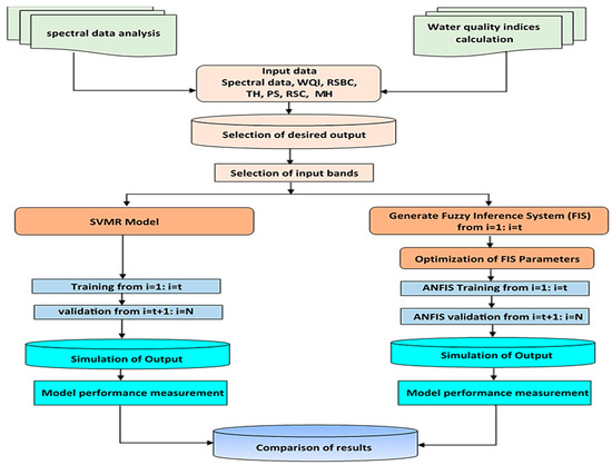
Figure 2.
Schematic diagram of the methodology of support vector machine regression (SVMR) and adaptive neuro-fuzzy inference system (ANFIS) used in this study for estimating the groundwater quality variables. WQI, RSBC, TH, PS, RSC, and MR indicate water quality index, residual sodium bicarbonate, total hardness, potential salinity, residual sodium carbonate, and magnesium hazard, respectively.
ANFIS Model
The ANFIS model is an FIS that is formulated as a feed-forward neural network. Thus, the advantages of a fuzzy system can be combined with learning algorithms [57]. Another benefit is that it can be amalgamated with learning algorithms [58,59]. By utilizing different output or input data, the ANFIS hypothesizes an FIS and typically modifies its membership function constraints on the basis of a backpropagation algorithm [60], and consequently, FIS may perhaps extract knowledge from the data used in training. Figure 3 represents the distinctive structural design of the ANFIS, which has a multilayered feed-forward setup and is connected to an incoherent network for the x as well as the y inputs. It is important to note that FIS is primarily made up of five functioning blocks.
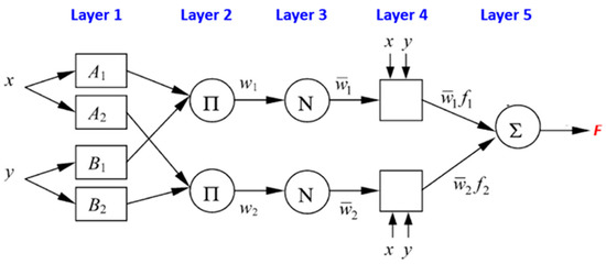
Figure 3.
Schematic diagram of the two rule Sugeno system ANFIS architecture.
The Sugeno model has a rule base with the following form:
In this particular case, fi is the output inside the incoherent zone and is denoted by the fuzzy principle; Ai and Bi are the membership values; a and b are indirect identifying functions; and pi, qi, and ri are the consequential restrictions, which are brought up to date within the forward pass inside the learning algorithm.
If the membership functions of the fuzzy sets Ai and Bj are correspondingly and , the five layers that incorporate ANFIS will be formulated as discussed below.
If the throughput of the layer one ith node is represented by O1,i, then for Layer 1, each node i is considered adaptive for the node function.
with a and b being the inputs to the node, and or is considered a function determined by past occurrences.
Layer 2 has nodes that are labeled and multiply the signals that enter the system. Each of the node’s throughputs denotes a rule’s firing strength:
Layer 3: Nodes that are labeled N in this layer scale the firing strengths to ensure the provision of the firing strengths is normalized:
Layer 4: Its output consists of a linear amalgamation of the inputs proliferated by the firing power, which are normalized. The layers of these nodes are adaptive and have specific roles:
where wi is the layer three output and a parameter set (pi, qi, ri). The parameters of Layer 4 are termed the resultant parameters.
Layer 5: It has a node and calculates the absolute output by considering the total of every inward bound signal:
Each square-illustrated layer is termed adaptive, and its values are typically changed while system training is conducted. Conversely, the layer epitomized by the circle remained invariable before, during, and after the training is complete. Figure 3 represents the network used in this study and comprises select bands as inputs, as well as one output membership function for the desired index (different irrigation water quality variables).
In this study, ANFIS was used to excerpt the relationship of spectral reflectance data and groundwater quality variables and characterize them as fuzzy “if–then” relationships. The postulate segment of fuzzy if–then rules includes spectral reflectance data. The consequential segment comprises the WQI, RSBC, TH, PS, RSC, and MR. The framework of the developed ANFIS archetype comprised a fuzzy system of the Sugeno type with a linear output membership function and a typical bell input membership function. The ANFIS simulation model contains two phases. The first corresponds to when operation rules are created using a fuzzy approach, and then, the already created FIS is applied as an input into the ANFIS system (Figure 4). For the second phase, the irrigation water quality variables were simulated using the final FIS, which was created using ANFIS.
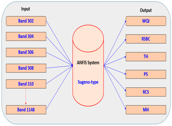
Figure 4.
An ANFIS architecture for prediction of groundwater quality variables. WQI, RSBC, TH, PS, RSC, and MR indicate water quality index, residual sodium bicarbonate, total hardness, potential salinity, residual sodium carbonate, and magnesium hazard, respectively.
SVMR Model
The SVMR algorithm is a universal theory of machine learning for pattern classification and recognition. The SVMR model can solve either regression or classification problems or can map both low-dimensional nonlinear inputs and high-dimensional linear outputs with excellent results. The SVMR model used spectra reflectance bands as input data in the spectrum and different groundwater quality variables as output data to establish calibration equations and used cross-validation to minimize over-fitting.
Performance Evaluation of the Developed Models
Different goodness-of-fit measures were used to evaluate the prediction of the ANFIS and SVMR models’ operation to predict the groundwater quality variables. Some of the measures that were utilized comprised the coefficient of determination (R2), Nash–Sutcliffe coefficient (E), RMSE, and MAD. A t-test (two-sample) of the averages was conducted to determine if there was a substantial difference between the simulated data and mean from the experiment.
The proposed Nash and Sutcliffe [61] efficiency was computed, as is shown below:
where is the average of the considered parameter.
The MAD evaluates the mean magnitude of the errors across a set of simulations, with no consideration of direction. It also gauges the precision of constant variables and is computed as is shown below:
where WQIo is the observed value and n is the number of data points. Meanwhile, the WQIf is the predicted value.
The absolute variance fraction, R2, is calculated as follows:
The variables must already be defined.
The RMSE demonstrates the fit (absolute) of the model to the data points (how the experimental data are closer to the model’s projected values). The RMSE measures the best of the absolute value, with the smaller RMSE values indicating the best fit and R2 being a relative measure of the fit. The RMSE is determined with the following formula:
The correlation coefficient is a statistical hypothesis that can be ascribed to the evaluation of how trends in the simulated values correspond to the inclinations in the experimental values (actual values). The formula for calculating the correlation coefficient is as follows:
3. Results and Discussion
3.1. Interpretation of Groundwater Quality through Physiochemical Parameters Using a Multivariate Analysis
The integration of multivariate statistical analysis approaches such as FA and PCA and a large set of physiochemical parameters has been widely applied as an effective strategy for providing meaningful information regarding water quality and sustainably managing water resources [17,19,20,62,63,64,65]. For instance, FA is a powerful tool that is used to reduce the complexity of several physiochemical parameters without losing a great deal of information from the original measurements. This appreciable reduction in physiochemical parameters is highly necessary for the superior interpretation of the original measurements as well as for reduced costs of laboratory measurements of these [66]. Generally, this tool is used in conjunction with physiochemical parameters to create new factor loadings. These factor loadings always have a strong relationship with the original physiochemical parameters. The factor loadings are classified as strong, moderate, and weak if their absolute values for physiochemical parameters are greater than 0.75, 0.75–0.50, and 0.50–0.30, respectively [67,68]. In this study, the FA reduced the 11 physiochemical parameters into two main factors (eigen value > 1) in both regions. These two factors explained, respectively, 73.6% and 57.7% of the total variability of the physiochemical parameters in the WD and CND regions (Table 2). The first factor accounted for 47.9% of the total variability and had strong loadings for TDS, K+, Na+, Cl−, and SO42− and moderate loadings for Mg2+ and Ca2+ in the WD region. By contrast, in the CND region it accounted for 40.8% of the total variability and had strong loadings for TDS, Ca2+, SO42−, and HCO3−, moderate loadings for Mg2+, and weak loadings for the temperature, K+, and Na+ (Table 2). The second factor accounted for 25.7% and 16.9% of the total variability in WD and CND regions, respectively, and had strong loadings for NO3− and weak ones for the pH in both regions. This factor also had strong loadings for HCO3− and Cl− in the WD and CND regions, respectively (Table 2).
Table 2.
Factor loading after varimax rotation, eigen values, variability (%), and cumulative (%) of different physicochemical parameters for groundwater samples collected from the Western Desert and Central Nile Delta. The values of all parameters are expressed in mg l−1 except for temperature (°C) and pH.
Additionally, the PCA was applied for the 11 physiochemical parameters to confirm the results of the FA. The primary objective of the PCA is to classify the different physiochemical parameters into major components such that the parameters that are their vectors, adjacent or parallel to each other and with a small angle between them, signify the strength of their reciprocal association. By contrast, the divergence of the vectors of the parameters expresses weak relationships between them. Based on the angles between the vectors of the parameters in the biplot of the PCA, the 11 physiochemical parameters were divided into three and four groups in the WD and CND regions, respectively (Figure 5). The first of these included K+, Ca2+, Mg2+, Na+, Cl−, SO42−, and TDS from the WD region, whereas that for the CND region included Ca2+, Mg2+, SO42−, HCO3−, and TDS. The second group, which only appeared in the CND region, comprised K+, Na+, and Cl−. The NO3− with HCO3− in the WD region and with a pH in the CND region was located in the third group. The fourth group contained pH and temperature in the WD region but only temperature in the CND region (Figure 5).
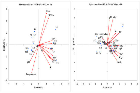
Figure 5.
Biplot of the principle component analysis for the first two components of different physicochemical parameters for groundwater samples collected from the Western Desert (WD) and Central Nile Delta (CND). S indicates samples.
Based on the final results of the FA and PCA, the following conclusions can be reached: (1) the TDS, which is an indicator of the salinity level and reflects the total concentrations of the dissolved cations and anions in water, was closely related to salt ions (principally, Na+, Cl−, and SO42−), as well as K+, Ca2+, and Mg2+ in the WD region, whereas it appeared to be associated with Ca2+, Mg2+, SO42−, and HCO3− in the CND region (Figure 5), wherein the salt ions exhibited stronger loadings for the first factor in the WD region than in the CND one; the opposite was true for Ca2+ and Mg2+ (Table 2); (2) the two cations (K+ and Na+), in which the ratio between both ions plays a distinctive role in the groundwater quality, particularly pertaining to their use as an irrigation water source, had strong and weak loadings for the first factor in the WD and CND regions, respectively, with the angle between the vectors of the two parameters being very close in both (Table 2 and Figure 5); (3) the NO3− had strong loadings (>0.77) for the second factor in both regions (Table 2) and was also plotted separately in individual groups with HCO3− in the WD region and pH in the CND one (Figure 5), which indicated that both point sources such as agricultural fertilizers, domestic waste, and anthropogenic activities, as well as non-point sources, such as agricultural runoff, soil erosion, and atmospheric deposition due to natural weathering, could be the source of NO3− in both regions; and (4) the pH in both regions and temperature in the CND region were less important in accounting for groundwater quality, as they showed a weak loading for either the first or second factor (Table 2) and also provided a large angle between their vectors and those of the other parameters (Figure 5). All of these findings indicate that the PCA mostly confirmed the FA results and, additionally, the combination of both methods was found to be advantageous to examining and interpreting the behavior of groundwater quality in both regions, as well as to predicting the variables that may impact groundwater quality by illuminating the relationship between physiochemical parameters and the factors or components of both analyses. The final results of both methods indicate that the groundwater of WD is less suitable for irrigation, whereas the first factor of FA exhibits strong loadings for TDS and salt ions (principally, Na+, Cl−, and SO42−), and moderate loadings for Ca2+ and Mg2+ (Table 2), as well as the salt ions, which make a major contribution to the TDS of the water, showed a small angle between their vectors and those of the TDS (Figure 5). The strong loadings of the salt ions in the groundwater of the WD may be attributed to the recharge from the underlying fractured limestone of the Eocene aquifer through hydraulic connection, as well as agricultural runoff into the quaternary aquifer system, which is considered as the most important aquifer in the WD region [69,70]. The moderate loadings of Ca2+ and Mg2+, compared with Na+ and Cl−, are also the result of the high mineralization processes through rock–water interaction such as reverse ion exchange, leaching, dissolution and precipitation processes [66,71]. Additionally, the excessive use of artificial chemical fertilizers and pesticides and the over-pumping of groundwater for irrigation, especially during summer seasons, may also lead to an increase in salinity hazards in the groundwater of the WD [72]. Therefore, this source of water can be used for irrigation purposes but with proper water management, such as the provision of a good drainage system and calculation of the water leaching requirements to control salt accumulation in the soil. The low or moderate loadings of salt ions in the groundwater of the CND region may be attributed to the Nile river’s water as the main source of water recharge in the area via seepage from the river’s two branches [17,73].
3.2. Validity of Groundwater for Irrigation Purposes
The evaluation of groundwater quality for irrigation purposes plays a fundamental role in the sustainability of soil health and crop productivity, especially in arid and semiarid conditions. Several IWQIs pertain to the suitability of any water source for irrigation purposes. Based on these indices, the quality of irrigation was classified into different classes to consider the risk of salinity problems, ion toxicity to plants, and soil permeability and degradations [9,12,17].
The WQI has been widely used for many decades to evaluate the suitability of groundwater for different usage purposes. The primary idea of this index is to integrate several physiochemical parameters into a single value to quickly and easily interpret the groundwater quality [4,8,74,75]. Importantly, this index can help with evaluating the key indicators relevant to groundwater quality in a comprehensive manner by highlighting the physiochemical parameters, which are highly important for irrigation water quality, and omitting the less important parameters. According to Meireles et al. [4], groundwater with a WQI value ranging from 85 to 100 can be safely used to irrigate the majority of soils with low probability of causing sodicity and salinity problems, and thus no toxicity risk for most field crops. The groundwater with WQI ranging from 70 to 85 is recommended for use to irrigate soils with high texture or moderate permeability with avoiding use for the irrigation of salt-sensitive crops. When the value of WQI ranged from 55 to 70, the groundwater can be used to irrigate the soils with moderate to high permeability values and irrigate the moderately salt-tolerant crops. However, if the value of WQI for groundwater ranged from 0 to 40, the water should be avoided to use for irrigation under normal conditions, and in special cases, it may be used occasionally. In this study, the groundwater samples of the CND exhibited higher values for WQI than those in the WD (Table 3). Furthermore, most of the groundwater samples from the CND region (72%) were categorized as having no restriction, and the remaining samples (28%) were categorized as having a low restriction. By contrast, 47% and 33% of the groundwater samples from the WD region fell in the high restriction and severe restriction categories, respectively (Table 4). These results indicate that the groundwater of the CND region was fresher than that of the WD region and therefore more suitable for irrigation purposes and human consumption. By contrast, the groundwater of the WD region can be safely used to irrigate soils that have coarse and medium textures, moderate the permeability status, and, with a good drainage system, calculate the water leaching requirements.
Table 3.
Statistical description of different irrigation water quality indices including water quality index (WQI), residual sodium bicarbonate (RSBC), total hardness (TH), potential salinity (PS), residual sodium carbonate (RSC), and magnesium hazard (MH) of groundwater samples collected from the Western Desert and Central Nile Delta.
Table 4.
Classification of groundwater quality based on different irrigation water quality indices (IWQIs) including water quality index (WQI), residual sodium bicarbonate (RSBC), total hardness (TH), potential salinity (PS), residual sodium carbonate (RSC), and magnesium hazard (MH) of groundwater samples collected from the Western Desert (WD) and Central Nile Delta (CND).
When soil is irrigated with high-RSC water, which measures the relationship in the sum concentration of CO32− and HCO3− to the sum of Ca2+ and Mg2+, soil degradation can result and crop productivity be negatively impacted due to the deposition of Ca2+ and Mg2+, as well as the sodium hazard in the soil potentially increasing [9,10,11]. Groundwater with an RSC value greater than 2.5 is harmful and unsuitable for irrigation purposes, whereas that with an RSC value of <1.25 is recommended as being safe for irrigation purposes. In this study, the RSC values of groundwater for the WD and CND regions ranging from −35.54 to 0.74 meq L−1 and from −6.34 to 0.29 meq L−1, respectively (Table 3). Furthermore, all groundwater samples from both regions were classified as good water and suitable for irrigation without limitations due to the RSC (Table 4). Additionally, all groundwater samples from both regions, except for one sample from each, featured negative RSC values that revealed excessive concentrations of Ca2+ and Mg2+ in the groundwater in both regions, without the potential build-up of Na+.
An excess of HCO3− concentrations in irrigation water negatively affects soil permeability and drainage, as well as the plant uptake of nutrients. Therefore, RSBC is an important IWQI for evaluating the suitability of groundwater for irrigation purposes based on HCO3− concentrations [5]. The RSBC values of groundwater for the WD and CND regions ranged from −17.42 to 3.76 meq L−1 and −3.7 to 1.28 meq L−1, respectively (Table 3). Furthermore, 100% of the groundwater samples from both regions met the requirement of water quality for irrigation purposes, all of their RSBC values being <5 meq L−1 and thus fell within the satisfactory category (Table 4).
A high level of Mg2+ concentrations in irrigation water leads to soil alkalinity, causes soil infiltration issues, decreases the availability of phosphorous, and ultimately diminishes crop productivity [49,63,76]. Therefore, MH was proposed for the evaluation of groundwater for the purpose of irrigation. The groundwater contains MH < 50 and was considered safe and suitable for irrigation purposes, with the opposite holding true for MH > 50 [77]. The MH values of the groundwater samples from the WD and CND ranged from 28.47% to 61.36%, and 12.38% to 44.18%, with 60% and 100% of the samples being safe for irrigation, respectively (Table 3 and Table 4).
PS is another IWQI for the classification of groundwater sources for irrigation. Generally, groundwater is considered safe for irrigation if its PS value is lower than 3 meq L−1 [13]. Only 13% of groundwater samples from WD were classified as being excellent to good, whereas most of the samples (80%) were classified as injurious to unsatisfactory. By contrast, 84% of groundwater samples from the CND were classified as excellent to good, with 4% classified as injurious to unsatisfactory (Table 4). This indicates that the groundwater of the CND has high suitability for irrigation purposes, whereas that of the WD can be used for irrigation, but with a proper water management system (i.e., providing a good drainage system and calculating water leaching requirements) to control salt accumulation in the soil.
The suitability of groundwater for irrigation purposes can also be evaluated by TH, which is mostly caused by the presence of Ca2+ and Mg2+ [78,79]. Usually, Ca2+ and Mg2+ are found in groundwater in the form of CaCO3 and CaMg(CO3)2, respectively. Therefore, groundwater with a TH level of more than 300 mg L−1 equivalent to CaCO3 will be problematic for the plumbing of irrigation systems [80]. The TH values of the groundwater from the WD and CND regions ranged, respectively, from 299.6 to 2213.8 mg L−1 and 299.6 to 2213.8 mg L−1 (Table 3). Furthermore, most groundwater samples from the WD region fell under the very hard category, whereas 52% of groundwater samples from the CND region fell under the same category and 36% fell under the hard one. None of the groundwater samples from the WD region fell under the moderately hard category, with 12% of the samples from the CND region falling under this category (Table 4).
3.3. Hyperspectral Characteristics of the Groundwater
Figure 6 displays the behavior of the spectral reflectance signature of the different groundwater samples collected from the two regions of between 302 and 1148 nm. The figure shows that there are obvious differences in the shape of the spectral reflectance curves between the samples. However, the spectral reflectance of the groundwater samples from the CND region was higher than that in the samples obtained from the WD one. Additionally, the figure also shows that the spectral reflectance curves of the two regions reveal three reflectance deep troughs around 320–340, 740–780, and 950–1000 nm wavelength regions and three reflectance peaks around 400–700, 780–820, and 1100–1148 nm wavelength regions (Figure 6). Furthermore, clear differences in the spectral reflectance between the groundwater samples in both regions were considerably large in the 302–318, 350–700, 750–900, and 1074–1148 nm wavelength regions. These results indicate that the obvious differences in physiochemical characteristics between the groundwater samples influenced the variations in the curves of the hyperspectral reflectance at different wavelength regions. Therefore, these results further suggest that it is possible to evaluate the parameters related to IWQIs in terms of the spectral characteristics of the water surface in these wavelength regions.
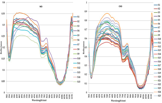
Figure 6.
Spectral reflectance signature of the different groundwater samples collected from the Western Desert (WD) and Central Nile Delta (CND).
The results displayed in Figure 7 further confirm this and test the strength of the relationship between the original spectral reflectance data throughout the entire wavelengths (302 to 1148 nm) and the six parameters related to the IWQIs using the pooled data of 40 groundwater samples. Generally, the WQI, RSC, and RSBC were positively correlated with the original spectral reflectance throughout the entire wavelengths, whereas the PS, TH, and MR parameters displayed the opposite relationships (Figure 7). Furthermore, the original spectral reflectance exhibited the highest correlation coefficients (r), with WQI (r = 0.24–0.84), followed, in sequence, by TH (r = 0.16–0.63), MR (r = 0.30–0.62), RSC (r = 0.15–0.60), and PS (r = 0.17–0.57). The RSBC was the least correlated with the original spectral reflectance (r = 0.09–0.43). Additionally, the highest correlation between the six IWQI parameters and the original spectral reflectance was located at wavelength intervals of 302–318, 358–900, and 1074–1148 nm, where the correlation coefficients between these wavelength regions and the WQI, RSC, RSBC, PS, TH, and MR were higher than 0.70, 0.50, 0.35, 0.49, 0.52, and 0.57, respectively (Figure 7). These findings confirm that the wavelengths with high correlation coefficient values can be useful for the spectroscopic analysis and quantification of water quality parameters. The results from the studied articles fully confirm this statement and have indicated a higher and consistent association between the spectral reflectance of the surface water at various parts of the spectrum and several water quality indicators. For instance, Ma and Dai [81] found that the spectral reflectance in the range between 760 and 1100 nm was the optimal wavelength interval for estimating the TSS concentrations. Wu et al. [82] demonstrated that the spectrum in the wavelengths ranging from 750 to 900 nm showed a strong correlation with the total TSS and turbidity values. The spectrum in the wavelengths ranging from 400 to 900 nm was found to be effective for estimating the concentrations of turbidity, phosphorus, BOD, and COD [22,30,44,83]. Xing et al. [28] also reported that the best wavelengths for estimating different water quality parameters included COD, BOD, TH, TA, and TDS were located in the spectrum ranging from 400 to 450 nm and from 900 to 1300 nm.
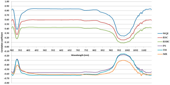
Figure 7.
Correlation coefficient between the original canopy spectral reflectance of the full wavelengths range (302–1148 nm) and different irrigation water quality indices (IWQIs) including water quality index (WQI), residual sodium bicarbonate (RSBC), total hardness (TH), potential salinity (PS), residual sodium carbonate (RSC), and magnesium hazard (MH).
3.4. Data-Driven Spectral Modeling for Predicting the Numerical Values of IWQIs
Performance of the Developed Models for Predicting the IWQIs
Since the relationships between the full range of the spectrum and IWQIs generated a wide range of effective wavelengths and the highest and most significant r values for these wavelengths were relatively flat, as is shown in Figure 7, it was difficult to develop effective models for estimating the water quality parameters based on the r using the full spectrum wavelengths. Moreover, although the simple spectral reflectance indices (SRIs, which focus on only two to three specific wavelengths), are widely used to estimate several IWQIs [23,27,29], this approach ignores a large number of wavelengths within the full spectrum, thereby causing small variations in the results or highly concentrated results. Furthermore, due to the large variation in environmental conditions and concentrations and types of water components reported in other studies, several published SRIs should be validated or new ones need to be derived, which would impose a heavy computational burden. As a result of the above-mentioned limitations of the methods of the Pearson correlation coefficient and SRIs for the accurate estimation of different IWQIs, therefore, several hyperspectral statistical models have recently been developed and gradually applied to improving the accuracy of IWQIs estimation. This study considered different ANFIS and SVMR models that are based on several spectral wavelengths in different spectrum regions to improve the estimation of the different IWQIs.
In this study, the two models of ANFIS and SVMR were utilized to develop the models for the simulation of the IWQIs. To construct both models, the IWQI datasets were randomly split into two sets of progressions, such as training and testing, by considering 70% and 30%, respectively. For the ANFIS models, subtractive clustering was used to create an FIS of a Sugeno-type. Furthermore, the separate input and output sets of the data-generated input arguments were then applied to the IWQIs. The primary purpose of implementing this step was to pinpoint the most appropriate antecedent membership functions, as well as the number of rules. The subsequent step encompassed the utilization of the linear least-squares estimation to determine the subsequent estimation of every rule’s equation to cover the feature space. Once the model of the best performance had been chosen via the ANFIS training, the predicted values of the selected output would be calculated, and a comparison made between these values and the actual values measured to estimate output (Supplementary Figures S1–S3 and Table 5). For instance, Supplementary Figure S1 displays the WQI values that were predicted by the ANFIS against the resultant experimental values for the training dataset as well as for testing. It is apparent in Supplementary Figure S1 that the two curves of estimated as well as experimental data nearly overlap one another, and this trend between the simulated and experimental data is similar apart from the few records that deviate by more than the actual experimental values. Table 5 summarizes the training, analysis, and corroboration of the output for the IWQIs prediction models. Clearly, the ANFIS carries outfitting, and the general projection upshots are objectively virtuous from the standpoints of R2, RMSE, MAD, and E. The large value of R2 is an indication of a perfect rapport between the projected and observed values of the IWQIs. Moreover, the RMSE is equal or closer to the MAD, which denotes that every error is of the same magnitude. A significant positive relationship was also obtained between the two measured and simulated WQIs in case of training and testing values. According to Equation (11), the range of E lies between 1.0 (perfect fit) and −∞; the high value of E is indicative of a more efficient data-driven model. Values of E in the range (−∞, 0) occur when the mean observed value is a superior estimation to the model’s prediction or a simulated value, which indicates inadequate performance. The values of E presented in Table 5 are above 0.85, which shows that the developed model is an ideal fit for WQI in terms of the testing and training datasets.
Table 5.
Comparison of statistical parameters between adaptive neuro-fuzzy inference system (ANFIS) and support vector machine regression (SVMR) models of measured and simulated values of different irrigation water quality indices (IWQIs) including water quality index (WQI), residual sodium bicarbonate (RSBC), total hardness (TH), potential salinity (PS), residual sodium carbonate (RSC), and magnesium hazard (MH).
Table 5 shows the R2, RMSE, MAD, and E of the training and testing datasets of the ANFIS and SVMR models based on all of the spectrum wavelengths for each IWQI. Generally, the ANFIS models offer a more accurate estimation of the different IWQIs in both the training and testing datasets (R2 was 1.00 in the training datasets and from 0.74 to 0.98 in the testing ones) than those from the SVMR models (R2 ranged from 0.29 to 0.88 in the training datasets and from 0.01 to 0.70 in the testing ones). The ANFIS models presented to lower the values for the RMSE and MAD and increase the values for E of the IWQIs over those of the SVMR model. The ANFIS models indicate a robust estimation for the WQI, RSC, RSBC, TH, and PS and a moderate one for the MH in testing datasets. However, the SVMR model showed a strong estimation for WQI and RSC, a moderate estimation for the PS and TH, and a weak estimation for the RSBC and MR in the testing datasets (Supplementary Figures S4–S6 and Table 5).
These results indicate that the ANFIS or SVMR models based on different spectral bands from the full spectrum wavelengths can provide additional improvements to assess IWQIs and can be considered a unified method for remotely estimating constituent concentrations in water quality evaluations. This is due to the various models of ANFIS or SVMR, which contain numerous sensitive and effective wavelengths that cover all of the main variations in the water components and are directly linked to the key changes in the undesired water quality parameters. As in this study, Wang et al. [64] developed SVMR models on the basis of SRIs to predict the drinking water quality index (DWQI). The models were based on selected SRIs of derivative order (1.6) and found to better estimate the DWQI than alternatives, with an R2 of 0.92, an RMSE of 58.4, and a slope of the equation of 0.97. Xing et al. [28] reported that including the most sensitive wavelengths in the PLSR model increased the estimation efficiency of several wastewater quality parameters, such as the TH. Additionally, for estimates of single water quality parameters, Wang et al. [64] reported that the PLSR models, based on a spectral reflectance range from 400 to 900 nm, indicated the best predictive through cross-validation for both the TSS (R2 = 0.97, RMSECV = 1.91, and RPD = 6.64) and chlorophyll-a (R2 = 0.98, RMSECV = 6.15, and RPD = 7.44).
4. Conclusions
In this study, the different physiochemical parameters were incorporated into a multivariate analysis (FA and PCA) to better understand and interpret the major contributing parameters that influence the groundwater quality of two distinct regions (WD and CND). The suitability of the groundwater in both regions for irrigation purposes was also evaluated based on various IWQIs. The ANFIS and SVMR models based on the optimal spectral reflectance bands were also applied to develop a new algorithm that can predict and simulate the IWQIs of groundwater. The results reported herein indicate that the combination of FA and PCA analysis was found to be advantageous to examining and interpreting the behavior of groundwater quality in both of the regions investigated, as well as for predicting the variables that may impact groundwater quality through an understanding of the relationship between the physiochemical parameters and the factors or components of both analytical approaches. The final results of both methods indicate that the groundwater of WD is less suitable for irrigation, whereas the first factor of FA exhibits strong loadings for TDS and salt ions (principally, Na+, Cl−, and SO42−), and moderate loadings for Ca2+ and Mg2+, as well as the salt ions, which make a major contribution to the TDS of the water, showed a small angle between their vectors and those of the TDS. Therefore, the groundwater of WD region can be safely used to irrigate soils that have coarse and medium textures, moderate permeability, and good drainage systems, with the water leaching requirements also calculated. According to the IWQ, RSBC, PS, RSC, and MH, approximately 7.0%, 100.0%, 13.0%, 100.0%, and 60.0% of groundwater samples in the WD are suitable for irrigation purposes and classified as low restriction, satisfactory, excellent to good, good, and suitable, respectively. However, almost all (72–100%) groundwater samples of the CND are very suitable for irrigation. The highest correlation between the six IWQI parameters and the original spectral reflectance was located at wavelength intervals of 302–318, 358–900, and 1074–1148 nm, where the correlation coefficients between these wavelength regions and the WQI, RSC, RSBC, PS, TH, and MR were higher than 0.70, 0.50, 0.35, 0.49, 0.52, and 0.57, respectively. These findings confirm that the wavelengths with high correlation coefficient values can be useful for the spectroscopic analysis and the quantification of water quality parameters. The applicability and capacity of the ANFIS and SVMR models were investigated based on a dataset collected from groundwater wells in the quaternary aquifer located in the CND and WD. The ANFIS models offer a more accurate estimation of the different IWQIs in both the training and testing datasets (R2 was 1.00 in the training datasets and from 0.74 to 0.98 in the testing ones) than those from the SVMR models (R2 ranged from 0.29 to 0.88 in the training datasets and from 0.01 to 0.70 in the testing ones). The ANFIS models indicate a robust estimation for the WQI, RSC, RSBC, TH, and PS and a moderate one for the MH in testing datasets. However, the SVMR model showed a strong estimation for WQI and RSC, a moderate estimation for the PS and TH, and a weak estimation for the RSBC and MR in the testing datasets. Finally, the main conclusion of this study is that the integration of both ANFIS and SVMR with proximal remote sensing could provide a highly useful tool for the prediction of IWQIs. On the basis of our findings, we propose the developed models as simple tools for predicting IWQIs and onsite evaluations.
Supplementary Materials
The following are available online at https://www.mdpi.com/2073-4441/13/1/35/s1, Figure S1. Comparison between training series (a and c) and testing series (b and d) for water quality index (WQI) and residual sodium bicarbonate (RSBC) using the developed ANFIS model. Figure S2. Comparison between training series (a and c) and testing series (b and d) for total hardness (TH) and potential salinity (PS) using the developed ANFIS model. Figure S3. Comparison between training series (a and c) and testing series (b and d) for residual sodium carbonate (RSC) and magnesium hazard (MH) using the developed ANFIS model. Figure S4. Comparison between training series (a and c) and testing series (b and d) for water quality index (WQI) and residual sodium bicarbonate (RSBC) using the developed SVMR model. Figure S5. Comparison between training series (a and c) and testing series (b and d) for total hardness (TH) and potential salinity (PS) using the developed SVMR model. Figure S6. Comparison between training series (a and c) and testing series (b and d) for residual sodium carbonate (RSC) and magnesium hazard (MH) using the developed SVMR model.
Author Contributions
Conceptualization, M.G., S.E., M.K. and S.E.-H.; methodology, M.K., M.G., S.E. and S.E.-H.; software, M.K., Y.H.D., N.A.-S., M.U.T. and M.M.; validation, S.E.-H., M.K., S.E., M.G. and N.A.-S.; formal analysis, S.E.-H., M.K., S.E., M.G., Y.H.D., and M.M.; investigation, S.E.-H., S.E., M.K. and M.G.; resources, S.E.-H., S.E., M.G. and N.A.-S.; data curation, S.E.-H., M.G., S.E. and M.K.; writing—original draft preparation, S.E.-H., S.E., M.K. and M.G.; writing—review and editing, S.E.-H.; visualization, S.E., M.K., S.E.-H., M.G.; supervision, S.E.-H. and S.E.; project administration, M.G., S.E. and S.E.-H; funding acquisition, S.E.-H., Y.H.D. and N.A.-S. All authors have read and agreed to the published version of the manuscript.
Funding
The authors extend their appreciation to the Deputyship for Research & Innovation, “Ministry of Education” in Saudi Arabia for funding this research work through the project number IFKSURG-1435-032.
Data Availability Statement
The data presented in this study are fully available in this article and Supplementary Materials.
Acknowledgments
The authors extend their appreciation to the Deputyship for Research & Innovation, “Ministry of Education” in Saudi Arabia for funding this research work through the project number IFKSURG-1435-032 and to the Researchers Support & Services Unit (RSSU) for their technical support.
Conflicts of Interest
The authors declare no conflict of interest.
References
- Bora, M.; Goswami, D.C. Water quality assessment in terms of water quality index (DWQI): Case study of the Kolong River, Assam, India. Appl. Water Sci. 2017, 7, 3125–3135. [Google Scholar] [CrossRef]
- Sawyer, G.N.; McCarthy, D.L. Chemistry of Sanitary Engineers, 2nd ed.; McGraw Hill: New York, NY, USA, 1967; p. 518. [Google Scholar]
- Sundaray, S.K.; Nayak, B.B.; Bhatta, D. Environmental studies on river water quality with reference to suitability for agricultural purposes: Mahanadi river estuarine system, India-A case study. Environ. Monit. Assess. 2008, 155, 227–243. [Google Scholar] [CrossRef] [PubMed]
- Meireles, A.C.M.; De Andrade, E.M.; Chaves, L.C.G.; Frischkorn, H.; Crisostomo, L.A. A new proposal of the classification of irrigation water. Rev. Ciência Agronômica 2010, 41, 349–357. [Google Scholar] [CrossRef]
- Ravikumar, P.; Somashekar, R.K.; Angami, M. Hydrochemistry and evaluation of groundwater suitability for irrigation and drinking purposes in the Markandeya River basin, Belgaum District, Karnataka State, India. Environ. Monit. Assess. 2010, 173, 459–487. [Google Scholar] [CrossRef]
- Li, P.; Tian, R.; Liu, R. Solute Geochemistry and Multivariate Analysis of Water Quality in the Guohua Phosphorite Mine, Guizhou Province, China. Expo. Health 2018, 11, 81–94. [Google Scholar] [CrossRef]
- Şener, Ş.; Şener, E.; Davraz, A. Evaluation of water quality using water quality index (WQI) method and GIS in Aksu River (SW-Turkey). Sci. Total Environ. 2017, 584, 131–144. [Google Scholar] [CrossRef]
- Kachroud, M.; Trolard, F.; Kefi, M.; Jebari, S.; Bourrié, G. Water Quality Indices: Challenges and Application Limits in the Literature. Water 2019, 11, 361. [Google Scholar] [CrossRef]
- Xu, P.; Feng, W.; Qian, H.; Zhang, Q. Hydrogeochemical Characterization and Irrigation Quality Assessment of Shallow Groundwater in the Central-Western Guanzhong Basin, China. Int. J. Environ. Res. Public Health 2019, 16, 1492. [Google Scholar] [CrossRef]
- Selvakumar, S.; Ramkumar, K.R.; Chandrasekar, N.; Magesh, N.S.; Seenipandi, K. Groundwater quality and its suitability for drinking and irrigational use in the Southern Tiruchirappalli district, Tamil Nadu, India. Appl. Water Sci. 2017, 7, 411–420. [Google Scholar] [CrossRef]
- Joshi, D.M.; Kumar, A.; Agrawal, N. Assessment of the irrigation water quality of River Ganga in Haridwar District India. J. Chem. 2009, 2, 285–292. [Google Scholar]
- Li, P.; Wu, J.; Qian, H.; Zhang, Y.; Yang, N.; Jing, L.; Yu, P. Hydrogeochemical Characterization of Groundwater in and Around a Wastewater Irrigated Forest in the Southeastern Edge of the Tengger Desert, Northwest China. Expo. Health 2016, 8, 331–348. [Google Scholar] [CrossRef]
- Doneen, L.D. Notes on Water Quality in Agriculture; Published as A Water Science and Engineering; Paper 4001; Department of Water Science and Engineering, University of California: Oakland, CA, USA, 1964. [Google Scholar]
- Wang, Y.; Wang, P.; Bai, Y.; Tian, Z.; Li, J.; Shao, X.; Mustavich, L.F.; Li, B.-L. Assessment of surface water quality via multivariate statistical techniques: A case study of the Songhua River Harbin region, China. HydroResearch 2013, 7, 30–40. [Google Scholar] [CrossRef]
- Chen, R.; Ju, M.; Chu, C.; Jing, W.; Wang, Y. Identification and Quantification of Physicochemical Parameters Influencing Chlorophyll-a Concentrations through Combined Principal Component Analysis and Factor Analysis: A Case Study of the Yuqiao Reservoir in China. Sustainability 2018, 10, 936. [Google Scholar] [CrossRef]
- Prieto-Amparan, J.A.; Rocha-Gutiérrez, B.A.; Ballinas-Casarrubias, L.; Aragón, M.C.V.; Peralta-Pérez, M.D.R.; Pinedo-Alvarez, A. Multivariate and Spatial Analysis of Physicochemical Parameters in an Irrigation District, Chihuahua, Mexico. Water 2018, 10, 1037. [Google Scholar] [CrossRef]
- Abdel-Fattah, M.K.; Abd-Elmabod, S.K.; Aldosari, A.A.; Elrys, A.S.; Mohamed, E.S. Multivariate Analysis for Assessing Irrigation Water Quality: A Case Study of the Bahr Mouise Canal, Eastern Nile Delta. Water 2020, 12, 2537. [Google Scholar] [CrossRef]
- Singh, K.P.; Malik, A.; Mohan, D.; Sinha, S. Multivariate statistical techniques for the evaluation of spatial and temporal variations in water quality of Gomti River (India)-a case study. Water Res. 2004, 38, 3980–3992. [Google Scholar] [CrossRef]
- Kazi, T.G.; Arain, M.; Jamali, M.; Jalbani, N.; Afridi, H.; Sarfraz, R.; Baig, J.; Shah, A.Q. Assessment of water quality of polluted lake using multivariate statistical techniques: A case study. Ecotoxicol. Environ. Saf. 2009, 72, 301–309. [Google Scholar] [CrossRef]
- Hamzah, F.; Jaafar, O.; Jani, W.; Abdullah, S. Multivariate Analysis of Physical and Chemical Parameters of Marine Water Quality in the Straits of Johor, Malaysia. J. Environ. Sci. Technol. 2016, 9, 427–436. [Google Scholar] [CrossRef]
- Duan, W.; He, B.; Takara, K.; Luo, P.; Nover, D.; Sahu, N.; Yamashiki, Y. Spatiotemporal evaluation of water quality incidents in Japan between 1996 and 2007. Chemosphere 2013, 93, 946–953. [Google Scholar] [CrossRef]
- Song, K.; Li, L.; Li, S.; Tedesco, L.; Hall, B.; Li, L. Hyperspectral Remote Sensing of Total Phosphorus (TP) in Three Central Indiana Water Supply Reservoirs. Water Air Soil Pollut. 2011, 223, 1481–1502. [Google Scholar] [CrossRef]
- Vinciková, H.; Hanus, J.; Pechar, L. Spectral reflectance is a reliable water-quality estimator for small, highly turbid wetlands. Wetlands Ecol. Manag. 2015, 23, 933–946. [Google Scholar] [CrossRef]
- Gholizadeh, M.H.; Melesse, A.M.; Reddi, L. A Comprehensive Review on Water Quality Parameters Estimation Using Remote Sensing Techniques. Sensors 2016, 16, 1298. [Google Scholar] [CrossRef] [PubMed]
- Yang, Y.; Gao, B.; Hao, H.; Zhou, H.; Lu, J. Nitrogen and phosphorus in sediments in China: A national-scale assessment and review. Sci. Total Environ. 2017, 576, 840–849. [Google Scholar] [CrossRef] [PubMed]
- Bansod, B.; Singh, R.; Thakur, R. Analysis of water quality parameters by hyperspectral imaging in Ganges River. Spat. Inf. Res. 2018, 26, 203–211. [Google Scholar] [CrossRef]
- Elhag, M.; Gitas, I.Z.; Othman, A.; Bahrawi, J.; Gikas, P. Assessment of Water Quality Parameters Using Temporal Remote Sensing Spectral Reflectance in Arid Environments, Saudi Arabia. Water 2019, 11, 556. [Google Scholar] [CrossRef]
- Xing, Z.; Chen, J.; Zhao, X.; Li, Y.; Li, X.; Zhang, Z.; Lao, C.; Wang, H. Quantitative estimation of wastewater quality parameters by hyperspectral band screening using GC, VIP and SPA. PeerJ 2019, 7, e8255. [Google Scholar] [CrossRef]
- Gad, M.; El-Hendawy, S.; Al-Suhaibani, N.; Tahir, M.U.; Mubushar, M.; Elsayed, S. Combining Hydrogeochemical Characterization and a Hyperspectral Reflectance Tool for Assessing Quality and Suitability of Two Groundwater Resources for Irrigation in Egypt. Water 2020, 12, 2169. [Google Scholar] [CrossRef]
- Zhang, Q.; Yang, L.; Song, D. Environmental effect of decentralization on water quality near the border of cities: Evidence from China’s Province-managing-county reform. Sci. Total Environ. 2020, 708, 135154. [Google Scholar] [CrossRef]
- Wu, C.; Wu, J.; Qi, J.; Zhang, L.; Huang, H.; Lou, L.; Chen, Y. Empirical estimation of total phosphorus concentration in the mainstream of the Qiantang River in China using Landsat TM data. Int. J. Remote Sens. 2010, 31, 2309–2324. [Google Scholar] [CrossRef]
- Gitelson, A.; Garbuzov, G.; Szilagyi, F.; Mittenzwey, K.-H.; Karnieli, A.; Kaiser, A. Quantitative remote sensing methods for real-time monitoring of inland waters quality. Int. J. Remote Sens. 1993, 14, 1269–1295. [Google Scholar] [CrossRef]
- Liu, H.; Li, Q.; Shi, T.; Hu, S.; Wu, G.; Zhou, Q. Application of Sentinel 2 MSI Images to Retrieve Suspended Particulate Matter Concentrations in Poyang Lake. Remote Sens. 2017, 9, 761. [Google Scholar] [CrossRef]
- Daniel, E.B.; Camp, J.V.; LeBoeuf, E.J.; Penrod, J.R.; Dobbins, J.P.; Abkowitz, M.D. Watershed modeling and its applications: A state-of-the-art review. J. Hydrol. 2011, 5, 26–50. [Google Scholar] [CrossRef]
- Orouji, H.; Bozorg-Haddad, O.; Fallah-Mehdipour, E.; Mariño, M. Modeling of Water Quality Parameters Using Data-Driven Models. J. Environ. Eng. 2013, 139, 947–957. [Google Scholar] [CrossRef]
- Liu, Z.-J.; Weller, D. A Stream Network Model for Integrated Watershed Modeling. Environ. Model. Assess. 2007, 13, 291–303. [Google Scholar] [CrossRef]
- Solomatine, D.P.; See, L.; Abrahart, R. Data-Driven Modelling: Concepts, Approaches and Experiences. Hydrol. Model. 2008, 17–30. [Google Scholar] [CrossRef]
- Khadr, M.; Elshemy, M. Data-driven modeling for water quality prediction case study: The drains system associated with Manzala Lake, Egypt. Ain Shams Eng. J. 2017, 8, 549–557. [Google Scholar] [CrossRef]
- Rossel, R.A.V.; Behrens, T. Using data mining to model and interpret soil diffuse reflectance spectra. Geoderma 2010, 158, 46–54. [Google Scholar] [CrossRef]
- Walczak, B.; Massart, D. The Radial Basis Functions-Partial Least Squares approach as a flexible non-linear regression technique. Anal. Chim. Acta 1996, 331, 177–185. [Google Scholar] [CrossRef]
- Broomhead, D.; Lowe, D. Multivariable functional interpolation and adaptive networks. Complex Syst. 1988, 2, 321–355. [Google Scholar]
- Dogan, E.; Sengorur, B.; Koklu, R. Modeling biological oxygen demand of the Melen River in Turkey using an artificial neural network technique. J. Environ. Manag. 2009, 90, 1229–1235. [Google Scholar] [CrossRef]
- Ranković, V.; Radulović, J.; Radojević, I.; Ostojić, A.; Čomić, L. Neural network modeling of dissolved oxygen in the Gruža reservoir, Serbia. Ecol. Model. 2010, 221, 1239–1244. [Google Scholar] [CrossRef]
- Wang, X.; Zhang, F.; Ding, J. Evaluation of water quality based on a machine learning algorithm and water quality index for the Ebinur Lake Watershed, China. Sci. Rep. 2017, 7, 12858. [Google Scholar] [CrossRef] [PubMed]
- APHA (American Public Health Association). Standard Methods for the Examination of Water and Wastewater, 17th ed.; American Public Health Association: Washington, DC, USA, 2012. [Google Scholar]
- Eaton, F.M. Significance of Carbonates in Irrigation Waters. Soil Sci. 1950, 69, 123–134. [Google Scholar] [CrossRef]
- Horton, R.K. An index number system for rating water quality. J. Water Pollut. Control Fed. 1965, 37, 300–306. [Google Scholar]
- Ayers, R.; Westcot, D. Water Quality for Agriculture; Food and Agriculture Organization of the United Nations: Rome, Italy, 1985; p. 97. [Google Scholar]
- Gautam, S.K.; Maharana, C.; Sharma, D.; Singh, A.K.; Tripathi, J.K.; Singh, S.K. Evaluation of groundwater quality in the Chotanagpur plateau region of the Subarnarekha river basin, Jharkhand State, India. Sustain. Water Qual. Ecol. 2015, 6, 57–74. [Google Scholar] [CrossRef]
- Jolliffe, I.T. Principal Component Analysis, 2nd ed.; John Wiley & Sons Inc.: Charlottesville, VA, USA, 2002; pp. 150–166. [Google Scholar]
- Alberto, W.D.; Del Pilar, D.M.; Valeria, A.M.; Fabiana, P.S.; Cecilia, H.A.; Ángeles, B.M. de los Pattern Recognition Techniques for the Evaluation of Spatial and Temporal Variations in Water Quality. A Case Study. Water Res. 2001, 35, 2881–2894. [Google Scholar] [CrossRef]
- Abdullah, P.; Haque, M.Z.; Rahim, S.A.; Embi, A.F.; Elfithri, R.; Lihan, T.; Khali, W.W.M.; Khan, F.; Mokhtar, M. Multivariate Chemometric Approach on the Surface Water Quality in Langat Upstream Tributaries, Peninsular Malaysia. J. Environ. Sci. Technol. 2016, 9, 277–284. [Google Scholar] [CrossRef]
- Lawley, D.N.; Maxwell, A. Factor Analysis as a Statistical Method. J. R. Stat. Soc. 1962, 3, 209–229. [Google Scholar] [CrossRef]
- Morrison, D.F. Multivariate Statistical Methods; McGraw-Hill Book Company: New York, NY, USA, 1967; pp. 299–309. [Google Scholar]
- Hutcheson, G.D.; Nick, S. The Multivariate Social Scientist: Introductory Statistics Using Generalized Linear Models; SAGE: Thousand Oaks, CA, USA, 1999. [Google Scholar]
- Ted, A. Baumgartner. Reading Statistics and Research (5th ed.). Meas. Phys. Educ. Exerc. Sci. 2008, 12, 52–54. [Google Scholar]
- Zadeh, L.A. Outline of a New Approach to the Analysis of Complex Systems and Decision Processes. IEEE Trans. Syst. Man Cybern. 1973, Smc3, 28–44. [Google Scholar] [CrossRef]
- Aifaoui, N.; Deneux, D.; Soenen, R. Feature-based Interoperability between Design and Analysis Processes. J. Intell. Manuf. 2006, 17, 13–27. [Google Scholar] [CrossRef]
- Kuo, R.J.; Tseng, Y.S.; Chen, Z.-Y. Integration of fuzzy neural network and artificial immune system-based back-propagation neural network for sales forecasting using qualitative and quantitative data. J. Intell. Manuf. 2014, 27, 1191–1207. [Google Scholar] [CrossRef]
- Labani, M.M.; Kadkhodaie-Ilkhchi, A.; Salahshoor, K. Estimation of NMR log parameters from conventional well log data using a committee machine with intelligent systems: A case study from the Iranian part of the South Pars gas field, Persian Gulf Basin. J. Petrol. Sci. Eng. 2010, 72, 175–185. [Google Scholar] [CrossRef]
- Lehner, B.; Henrichs, T.; Döll, P.; Alcamo, J. EuroWasser: Model-based assessment of European water resources and hydrology in the face of global change. In Kassel World Water Series 5; Center for Environmental Systems Research, University of Kassel: Kassel, Germany, 2001. [Google Scholar]
- Hao, R.X.; Li, S.M.; Li, J.B.; Zhang, Q.K.; Liu, F. Water Quality Assessment for Wastewater Reclamation Using Principal Component Analysis. J. Environ. Inform. 2013, 21, 45–54. [Google Scholar] [CrossRef]
- Mirza, A.T.M.; Saadat, A.H.M.; Islam, M.S.; Al-Mansur, M.A.; Ahmed, S. Groundwater characterization and selection of suitable water type for irrigation in the western region of Bangladesh. Appl. Water Sci. 2017, 7, 233–243. [Google Scholar]
- Wang, J.; Zhou, W.; Pickett, S.T.; Yu, W.; Li, W. A multiscale analysis of urbanization effects on ecosystem services supply in an urban megaregion. Sci. Total Environ. 2019, 662, 824–833. [Google Scholar] [CrossRef]
- Ravikumar, P.; Somashekar, R.K. Principal component analysis and hydrochemical facies characterization to evaluate groundwater quality in Varahi river basin, Karnataka state, India. Appl. Water Sci. 2015, 7, 745–755. [Google Scholar] [CrossRef]
- Zeng, X.; Rasmussen, T.C. Application of multivariate statistical techniques in the assessment of water quality in the Southwest New Territories and Kowloon, Hong Kong. Environ. Monit. Assess. 2010, 137, 17–27. [Google Scholar]
- Liu, C.W.; Lin, K.H.; Kuo, Y.M. Application of factor analysis in the assessment of groundwater quality in a Blackfoot disease area in Taiwan. Sci. Total Environ. 2003, 13, 7789. [Google Scholar] [CrossRef]
- Unmesh, C.P.; Sanjay, K.S.; Prasant, R.; Binod, B.N.; Dinabandhu, B. Application of factor and cluster analysis for characterization of river and estuarine water systems—A case study: Mahanadi River (India). J. Hydrol. 2006, 331, 434–445. [Google Scholar]
- El Sheikh, A.E. Water Budget Analysis of the Quaternary Deposits for the Assessment of the Water Logging Problem of El Fayoum Depression. Ph.D. Thesis, Faculty of Science, Al-Azhr University, Cairo, Egypt, 2004; p. 233. [Google Scholar]
- Gad, M.; El-Hattab, M. Integration of water pollution indices and DRASTIC model for assessment of groundwater quality in El Fayoum depression, western desert, Egypt. J. Afr. Earth Sci. 2019, 158, 103554. [Google Scholar] [CrossRef]
- Gad, M.; El Osta, M. Geochemical controlling mechanisms and quality of the groundwater resources in El Fayoum Depression, Egypt. Arab. J. Geosci. 2020, 13, 1–23. [Google Scholar] [CrossRef]
- Ahmed, M.A. Assessment of intrinsic vulnerability to contamination for the Alluvial aquifer in El-Fayoum Depression using the DRASTIC method. J. Radiat. Res. Appl. Sci. 2012, 5, 743–768. [Google Scholar]
- Negm, A.M.; Sakr, S.; Abd-Elaty, I.; Abd-Elhamid, H.F. The Handbook of Environmental Chemistry; Springer Science and Business Media LLC: Cham, Switzerland, 2018; pp. 3–44. [Google Scholar]
- Lumb, A.; Sharma, T.C.; Bibeault, J.-F. A Review of Genesis and Evolution of Water Quality Index (WQI) and Some Future Directions. Water Qual. Expo. Health 2011, 3, 11–24. [Google Scholar] [CrossRef]
- Rocha, F.C.; De Andrade, E.M.; Lopes, F.B. Water quality index calculated from biological, physical and chemical attributes. Environ. Monit. Assess. 2014, 187, 4163. [Google Scholar] [CrossRef] [PubMed]
- Rawat, K.S.; Singh, S.K.; Gautam, S.K. Assessment of groundwater quality for irrigation use: A peninsular case study. Appl. Water Sci. 2018, 8, 233. [Google Scholar] [CrossRef]
- Khodapanah, L.; Sulaiman, W.N.A.; Khodapanah, D.N. Groundwater quality assessment for diferent purposes in Eshtehard District, Tehran, Iran. Eur. J. Sci. Res. 2009, 36, 543–553. [Google Scholar]
- Schroeder, H.A. Relations between hardness of water and death rates from certain chronic and degenerative diseases in the United States. J. Chronic Dis. 2004, 12, 586–591. [Google Scholar] [CrossRef]
- Sawyer, C.N.; McCarthy, P.L.; Parkin, G.F. Chemistry for Environmental Engineering and Science, 5th ed.; McGraw-Hill: New York, NY, USA, 2003. [Google Scholar]
- Nagaraju, A.; Kumar, K.S.; Thejaswi, A. Assessment of groundwater quality for irrigation: A case study from Bandalamottu lead mining area, Guntur District, Andhra Pradesh, South India. Appl. Water Sci. 2014, 4, 385–396. [Google Scholar] [CrossRef]
- Ma, R.; Dai, J. Investigation of chlorophyll-a and total suspended matter concentrations using Landsat ETM and field spectral measurement in Taihu Lake, China. Int. J. Remote Sens. 2005, 26, 2779–2795. [Google Scholar] [CrossRef]
- Wu, J.-L.; Ho, C.-R.; Huang, C.-C.; Srivastav, A.L.; Tzeng, J.-H.; Lin, Y.-T. Hyperspectral Sensing for Turbid Water Quality Monitoring in Freshwater Rivers: Empirical Relationship between Reflectance and Turbidity and Total Solids. Sensors 2014, 14, 22670–22688. [Google Scholar] [CrossRef] [PubMed]
- Jouanneau, S.; Recoules, L.; Durand, M.; Boukabache, A.; Picot, V.; Primault, Y.; Lakel, A.; Sengelin, M.; Barillon, B.; Thouand, G. Methods for assessing biochemical oxygen demand (BOD): A review. Water Res. 2014, 49, 62–82. [Google Scholar] [CrossRef] [PubMed]


Publisher’s Note: MDPI stays neutral with regard to jurisdictional claims in published maps and institutional affiliations. |
© 2020 by the authors. Licensee MDPI, Basel, Switzerland. This article is an open access article distributed under the terms and conditions of the Creative Commons Attribution (CC BY) license (http://creativecommons.org/licenses/by/4.0/).