Regression Models for Soil Water Storage Estimation Using the ESA CCI Satellite Soil Moisture Product: A Case Study in Northeast Portugal

Abstract

The European Space Agency Climate Change Initiative Soil Moisture (ESA CCI SM) product provides soil moisture estimates from radar satellite data with a daily temporal resolution. Despite validation exercises with ground data that have been performed since the product’s launch, SM has not yet been consistently related to soil water storage, which is a key step for its application for prediction purposes. This study aimed to analyse the relationship between soil water storage (S), which was obtained from soil water balance computations with ground meteorological data, and soil moisture, which was obtained from radar data, as affected by soil water storage capacity (Smax). As a case study, a 14-year monthly series of soil water storage, produced via soil water balance computations using ground meteorological data from northeast Portugal and Smax from 25 mm to 150 mm, were matched with the corresponding monthly averaged SM product. Linear (I) and logistic (II) regression models relating S with SM were compared. Model performance (r² in the 0.8–0.9 range) varied non-monotonically with Smax, with it being the highest at an Smax of 50 mm. The logistic model (II) performed better than the linear model (I) in the lower range of Smax. Improvements in model performance obtained with segregation of the data series in two subsets, representing soil water recharge and depletion phases throughout the year, outlined the hysteresis in the relationship between S and SM.

1. Introduction

Hydrological processes occurring on the Earth’s surface and interacting with the lower atmosphere are key to understanding atmospheric dynamics and climate change and their effects on the global water cycle. In this context, soil moisture is one of the essential climate variables (ECVs) [1,2] playing an important role in the climate dynamics [3] and change [4,5], the water cycle and the soil–atmosphere energy exchange [6]. In fact, it influences hydrological and agricultural processes, runoff generation [7], drought development and many other atmospheric processes, such as actual evapotranspiration [8] and their spatial and temporal variability [9,10,11,12].

Climate and vegetation feedbacks are linked to soil moisture, meaning that soil moisture changes have a direct impact on natural ecosystems, forests and farmland productivity [2]. Advances in soil water dynamics research related to atmospheric drivers contribute towards improved water management in agriculture, increased irrigation efficiency and enhanced food security, especially in arid and semiarid areas [13,14,15], as well as providing increasingly more robust tools for identifying and predicting potential impacts of soil moisture changes on ecohydrological processes at several temporal scales [6]. On the other hand, land-use changes affect the water balance components, especially the evapotranspiration related to precipitation and, therefore, the actual soil water storage dynamics throughout the vegetation cycles [16,17]. As such, the soil water balance is a valuable tool for analysing the impacts of land-use changes on soil water storage and to designing adaptation strategies for global change scenarios as far as water resources management is concerned.

For this, reliable hydrological data series are required, which is often a challenge in many regions worldwide, where data availability is scarce or nonexistent. In these areas, in situ hydrological monitoring networks are weakly developed and temporal series are insufficient to allow for spatially and temporally consistent appraisals of the water balance at the regional scale. Therefore, remote-sensing techniques and data sources help to overcome such constraints [18,19,20]. A considerable amount of technology is being applied in the remote monitoring and early detection of soil moisture status based on the water dielectric properties that can be detected with high precision in the microwave spectral region [21,22,23,24]. In addition, the signal does not suffer due to interferences from the composition of atmospheric gases or vegetation [25,26]. Furthermore, remote sensing research is exploring a wide range of applications that direct involve soil moisture, such as the prediction of vegetation water requirements [27], assessment of drought, hydrological [28,29] and agricultural measurements [30,31,32], estimation of the irrigation water demand by different crops [33] and flooding forecasts [24,34,35]. Furthermore, comparisons of different satellite products have been carried out to improve the performance of soil moisture remote assessment [36,37].

Several satellite missions are dedicated to monitoring soil moisture and providing continuous products worldwide. The Soil Moisture Climate Change Initiative (CCI) project is part of the European Space Agency (ESA) CCI. The ESA CCI Soil Moisture (SM) product has contributed to hundreds of hydrological and climatological studies worldwide. The latest release version of CCI Soil Moisture (v05.2) combines active and passive products from eight microwave-radiometer-based and four scatterometer-based products [38]. In particular, the microwave-radiometer-based products are from the Scanning Multichannel Microwave Radiometer (SMMR, 1979–1987), the Special Sensor Microwave Imager (SSM/I, 1987–2013), the TRMM Microwave Imager (TMI, 1998–2013), the Advanced Microwave Scanning Radiometer Earth observing system (AMSR-E, 2002–2011), the WindSat (2007–2012), the Advanced Microwave Scanning Radiometer (AMSR2, 2012–2019), the Soil Moisture and Ocean Salinity (SMOS, 2010–2019) and Soil Moisture Active and Passive mission (SMAP, 2015–2019). The scatterometer-based products are from the Active Microwave Instrument (AMI-WS ERS-1/2 SCAT, 1991–2006; AMI-WS ERS2, 1997–2007) and the Advanced SCATterometer (ASCAT) Metop-A (2007–2019) and Metop-B (2012–2019) [38]. The latter is sensitive to soil moisture, especially at low frequencies in the L-band (f = 1−2 GHz, λ = 30−15 cm) and C-band (f = 4−8 GHz, λ = 7.5−3.8 cm), since in this spectrum area, the soil dielectric constant reflects a proportional response to the water content in the surface layer and the best capacity of the L-band (1.4 GHz) to penetrate the vegetation layer [22,39]. One advantage of the ESA CCI SM combined product is that it provides larger spatial and temporal samples compared to single-sensor SM products [26]. Furthermore, the ESA CCI SM algorithm generates consistent, quality-controlled, long-term (1978–2019) soil moisture climate data records by harmonising and merging soil moisture retrievals from multiple radar satellites, including active and passive microwave-based signals with different frequencies; hence, different retrieval algorithms are used to generate the combined product [40,41].

The active and passive products are rescaled to a common time; then, they are inter-calibrated and merged into just one product on a pixel basis. Subsequently, the systematic differences between the active and passive products are corrected on a pixel basis [22]. The combined datasets (ESA CCI SM v05.2, Wien, Wien, Austria) span from 1978 to 2019, with a spatial resolution of 0.25 × 0.25°, a temporal resolution of ≈1 day and a soil thickness of ≈5 cm. The spatial resolution of the ESA CCI SM data is too coarse for some applications and downscaling techniques have been explored to obtain a finer spatial resolution (e.g., [42]). Several validation/prediction exercises of the ESA CCI SM data [26,41,42,43,44,45] have been done since the product was made available, for example, in drought studies [36,46], land–atmosphere interactions studies [47], climate trend analyses [40,48], detection of irrigated areas [49] and crop growth modelling [50]. Enlarging the geographical distribution of studies by applying the product certainly helps to widen the validation of SM estimates [51], especially in regions where the existing network of reference ground stations is sparse, as is the case in the western Iberian Peninsula [43].

The ESA CCI SM product provides soil moisture data in terms of the volumetric water content, while water balance appraisals operate with water volumes per unit surface area in the defined computation time interval (except for stream discharge), meaning that the soil water storage, a water balance output, is commonly expressed as an equivalent height. Satellite data products (e.g., Gravity Recovery and Climate Experiment (GRACE), Tropical Rainfall Measuring Mission (TRMM), Moderate Resolution Imaging Spectroradiometer (MODIS), Global Precipitation Climatology Center (GPCP), and others) have been used worldwide to estimate the water balance components (precipitation, evapotranspiration and water storage change) and to model the terrestrial water budget at the catchment scale [52,53,54,55,56,57,58,59]. The main source of uncertainty is related to precipitation data [53,55,57,58], while among the hydrological variables, evapotranspiration is one of the most difficult to reliably estimate [59]. Despite these constraints, satellite products have a large potential for assessing terrestrial water balance dynamics and for understanding their spatial and temporal variability at multiple scales [18]. Most studies referenced above used hydrological modelling based on water balance approaches applied at large spatial scales and a common conclusion was that the joint assimilation of soil moisture and total water storage remote data improves model performance [60,61,62]. Furthermore, the validation of radar products is commonly performed with meteorological data matrices that are obtained from satellite data, such as NOOA or Meteosat (e.g., [18,60,61,62,63,64,65]).

Table 1. Summary of relevant literature using satellite-derived soil moisture products.

Studies Using:	Data Assimilation in Land Surface Models		Comparison with Ground Soil Moisture Data
	Soil Water Storage as Output	Other Outputs
European Space Agency Climate Change Initiative Soil Moisture (ESA CCI SM) data	-	[26,29,45,46,47,48,49,50,62]	[25,36,37,40,41,42,43,44,47,51]
Other soil moisture remote sensing data	[60,61]	[24,31,33,34,63]	[21,30,31,32,40,41,66]

is presented to condense the relevant literature on the topic. From this, it is evident that research on the relationship between soil water storage, computed with ground meteorological data, and the ESA CCI SM combined product is still lacking.

In fact, water balance computations require the definition of a maximum soil water storage, or soil water storage capacity, whose effect on the relationship with SM is hardly reported in the literature [62,67]. This is an important and not yet fully explored issue that affects the use of satellite products measuring SM at smaller spatial scales, as the soil water storage capacity may present a wide range of spatial variation, depending on soil and crop characteristics [68]. On the other hand, a linear shape is commonly assumed in the relationships between the datasets issued from the different sources (satellite or ground), and regarding the different variables under consideration (soil moisture or soil water storage). Indeed, linearity is reported for the relationship between SM and the soil dielectric constant in most of the soil moisture range that is usually observed [69], as well as for that between total water storage and GRACE data [65]. No explicit support, other than statistical, is reported to justify the linearity assumption. Apart from the conventional approach of deriving statistical (data-driven) or functional (model-driven) relationships between datasets (matching remote data from different sources or matching remote data with ground sources), machine learning offers an alternative approach to generating large-scale soil moisture estimates by also using radar products, with promising results [66].

Considering such a research background, this paper presents a case study in NE Portugal that was specifically aimed at analysing the statistical relationship between soil water storage, which was obtained from soil water balance computations with ground meteorological data, and soil moisture, as given by the ESA CCI SM product. As part of the analysis, the study also aimed at assessing the effect of soil water storage capacity in this relationship. In its broader purpose, the research supporting this study is intended to contribute towards enlarging the set of application and ground validation exercises of the ESA CCI SM product with ground data from Portugal. It is worth stressing that this exercise is performed in an especially important region, namely, the Mediterranean, where soil water shortage, and its prospected aggravation, is a critical water management challenge. Since it is based on long-term data series, the research also intended to respond to the growing demand for reliable tools for predicting soil water storage from satellite-borne data while accounting for actual soil crop variability.

2. Materials and Methods

2.1. Study Area

The study was carried out in the Bragança area, NE Portugal (Figure 1). According to the Köppen–Geiger classification, the climate is temperate with dry and warm summers (Csb, Mediterranean type) [70,71], with the long-term annual averages of temperature and precipitation at Bragança being 12.3 °C and 758 mm, respectively [72]. Bragança is set in a mountain region with a roiling topography and strong regional climatic contrasts, ranging from humid and wet sub-humid at higher elevations (aridity index, i.e., the annual average precipitation to potential evapotranspiration ratio, AI > 0.65) to semiarid in the topographic depressions (AI < 0.5) [73]. The regional surface area facing severe susceptibility to desertification and drought has significantly increased in the last few decades [74,75]. Threats to natural resources, such as soil and water, prevail all over the region, namely, soil degradation processes associated with high potential erosion risk, which is boosted by frequent forest fires [76,77,78]. In fact, almost 73% of the Bragança District area presents a semiarid (19.7%, 0.2 < AI < 0.5) or dry sub-humid (53%, 0.5 < AI < 0.65) climate [74], with high and moderate susceptibility to desertification, respectively, and 38% of the soils are degraded [71,75], which is dominantly concentrated in desertification susceptibility areas.

The soil parent material is predominantly schist, although granite, mafic and ultra-mafic rocks are also found in the region [71]. The soils are mostly Leptosols (75.3%) [79], shallow and gravelly, dominantly medium-texture, acidic, with moderate to low organic matter content [80]. The land suitability for agriculture is dominantly marginal and limited by a low effective soil depth, high soil stoniness, steep slopes and severe soil water shortage, with the deficit season lasting for up to 8 months in the warmer, drier and lower elevation areas [71,75].

2.2. Soil Water Balance Estimation with Ground Data

Soil water balance calculations were performed with ground data recorded at Quinta de Santa Apolónia weather station (QSA), which is managed by and located in the campus of the Polytechnic Institute of Bragança (41°47′48″ N, 6°45′57″ W, 681 m elevation) (Figure 1).

The Thornthwaite method [81] was adopted to estimate the reference evapotranspiration (ETo) using the QSA weather station monthly mean air temperature. Although the United Nations Food and Agriculture Organization (FAO) recommends the Penman–Monteith method [82], the Thornthwaite method requires fewer input data (air temperature and location latitude) and applies a more straightforward calculation routine; therefore, it requires less robust datasets, which is beneficial when dealing with missing values is a common challenge. In fact, [54] used the Surface Energy Balance Algorithm for Land (SEBAL) to estimate ETo with the Penman–Monteith method from MODIS and TRMM satellite data, where they pointed out missing input data as a drawback for model validation. Moreover, in view of replication of the present study’s methodological approach and for results upscaling purposes, Thornthwaite ETo estimation requires the most commonly available large-scale datasets, which are too restrictive for the Penman–Monteith application.

Soil water balance computations followed the procedures of the Thornthwaite–Mather method [83,84]. Requiring monthly ETo and P (precipitation) values, the method outputs estimates of monthly soil water storage (S) and its changes (ΔS) throughout the year, together with real evapotranspiration (ETr), soil water deficit (WD) and superavit (WS). A maximum soil water storage must be defined a priori (Smax, millimetre equivalent depth), according to soil and crop characteristics, namely, available soil water capacity (AWC) and rooting depth (z) [83]. The reference Smax for climatic classification purposes is 100 mm [81].

The Thornthwaite–Mather method was applied using the QSA weather station monthly data for each year of the study period (January to December). The year totals of each input (P, ETo) and output variable (ETr, WD, WS) were also calculated. Deficit, superavit and recharge periods were identified, with the latter occurring when P − ETo > 0 and S < Smax, and the first two corresponding to the dry and wet seasons, respectively. For comparison purposes, the method was equally applied with the mean monthly P and ETo values of the study period and the climate normal (1971–2000). Procedures were repeated for Smax 150 mm (representing high soil water storage conditions), Smax 100 mm (representing reference Smax), and Smax 75, 50 and 25 mm (representing moderate–low, low and very low soil water storage, respectively), thus covering a wide range of soils (with different available water capacities) and/or crops (with different rooting depths). It should be added that soils of the study area are dominantly shallow, poor in organic matter and gravelly, and therefore better represented by the Smax lower range, while the upper range represents the scarce area assigned to deeper soils, such as Cambisols and Fluvisols [71,80].

2.3. ESA CCI Satellite Product

SM is an ESA CCI product (V 04.2) that utilises four active radar products (AMI WS, ERS-1/2 SCAT, MetOp-A+B ASCAT) and seven passive radar products (SMMR, SSM/I, TRMM, Windsat, AMSR-E, AMSR2, SMOS) microwave sensors; then, data is processed by the Microwave Remote Sensing Group at TU Wien [22,85]. The product is freely available in the Copernicus database (https://cophub.copernicus.eu/dhus/#/home), with a spatial resolution of 0.25°, a time resolution of 1 day and the data series started in 1978. The GIS SNAP (Sentinel Application Platform), version 6.0, a freely available tool found at http://step.esa.int/main/download/, was used for the satellite imagery processing.

Space and time attributes of the SM data were considered prior to comparisons with the ground data, which meant (i) appraising the representation in the SM pixel area of the ground climatic conditions, (ii) setting the study period for which the ground and satellite data were both available and (iii) representing the available daily SM data with a monthly time scale.

As expected in mountainous areas, the elevation is a major factor that determines the regional climate distribution, where for NE Portugal, the mean annual precipitation is positively correlated with elevation (r = 0.513), while the mean annual temperature and elevation are negatively correlated (r = −0.738), with the two climate elements varying inversely in the region (r = −0.559) [86]. Considering this, a 30 m resolution Digital Elevation Model (Advanced Land Observing Satellite (ALOS) World 3D—https://www.eorc.jaxa.jp/ALOS/en/aw3d/index_e.htm) was used to derive the elevation areal distribution in pixels, as depicted in Figure 1. The QSA elevation fell close to the pixel’s median (P50), with a 42 m difference for an effective altitudinal range of 327 m (P95 − P5, with P referring to percentile). Therefore, it was assumed that the QSA ground climatic conditions provided a good representation of those prevailing in the SM pixel area.

The selected SM data series extended for 14 years (2003–2016), which was the longest continuous timespan with simultaneously available ground and satellite-borne data. In fact, earlier than 2003, the ESA CCI SM product imagery existing for the area contains a large set of missing data in the daily SM series.

For obtaining a monthly SM data series, which is required for a comparison with the monthly water balance that is computed with the ground data, three randomly selected years were analysed in detail. For these, the monthly SM averages were computed (i) with daily data before and after the accumulated period of precipitation and (ii) with data of three fixed days: the 1st of the month, the 15th of the month and the 1st of next month. It should be noted that missing data commonly occurred in these years, meaning that the monthly averages were computed with the available data. Non-significant differences were found between the two sets of monthly averages, which showed very similar individual values and were strongly correlated (r = 0.896). These results encouraged the application of the procedure for the entire study period.

Furthermore, the SM pattern of evolution throughout the year and its changes during the study period were analysed. For this purpose, the SM series was divided into two subsets, each one assembling the SM rise and decline periods, corresponding to the soil water recharge or wetting periods and to the soil water depletion or drying periods, respectively. Soil water depletion occurs from the highest SM value in the wet season to the lowest at the end of the dry season, whereas soil recharge occurs in the remaining months of the year. For the entire study period, the drying data subset was larger than the wetting subset.

2.4. Regression Models

Monthly SM and water balance data for the study period (2003–2016) were summed up to give a total of 168 values for each variable. Regression analysis was performed between the satellite-borne and the ground data series, taking S (mm) as the variable that was dependent on SM (m³ m⁻³, converted to a percentage, %) due to the prediction purposes being explored in this research.

Two regression models were tested (S* stands for the S model estimate):

$$\mathrm{Model} \mathrm{I} \left(\mathrm{Linear}\right): S^{*}= a + b\mathrm{SM},$$

(1)

$$\mathrm{Model} \mathrm{II} (\mathrm{Logistic}): S^{*}=\frac{\mathrm{Smax}}{\left({1 + \mathrm{e}}^{a+b\mathrm{SM}}\right)}.$$

(2)

In model I, the dependent variable was bounded by the domain limits that were defined in the water balance computation (0 < S < Smax), meaning that all S estimates (S*) falling outside this range were set equal to the nearest domain limit (0 or Smax). The plots of SM against S suggested a non-linear relationship between these variables, and it was hypothesised that a logistic function (model II) would represent the relationship better than the linear function (model I). Furthermore, model II is asymptotically bounded to 0 and Smax, therefore providing a more realistic approach to the data range extremes than model I. Among other possible choices [87], the adopted logistic function [88] allowed for simple linearisation such that linear regression analysis was performed with its linearised form.

Regression analysis was performed with data from the entire study period (14 years), which involved testing the performance of the two models regarding statistically predicting S with SM data. As indicated earlier, water balance computations were repeated for a range of Smax values (25, 50, 75, 100 and 150 mm), which yielded the respective S series. Regression models were applied for the five soil water storage conditions in order to test the effect of Smax on the models’ performances. Regression analysis was also performed separately with the wetting and the drying data subsets to appraise differences between the subsets in the SM–S relationship. In this case, only model II was applied with the S data issued from water balance computations for the five soil water storage conditions. Finally, regression analysis was performed independently for each year of the study period using both models I and II in order to assess the interannual variability in the models’ performances and search for factors explaining this variability. This was done with the S data for all Smax conditions.

The models’ performances were evaluated using performance indicators, namely, the determination coefficient (r²), efficiency coefficient (CE), root mean square error (RMSE, mm) and standard error of the estimate (SEE, mm), which were all applied to the observed and estimated S data series [89].

3. Results

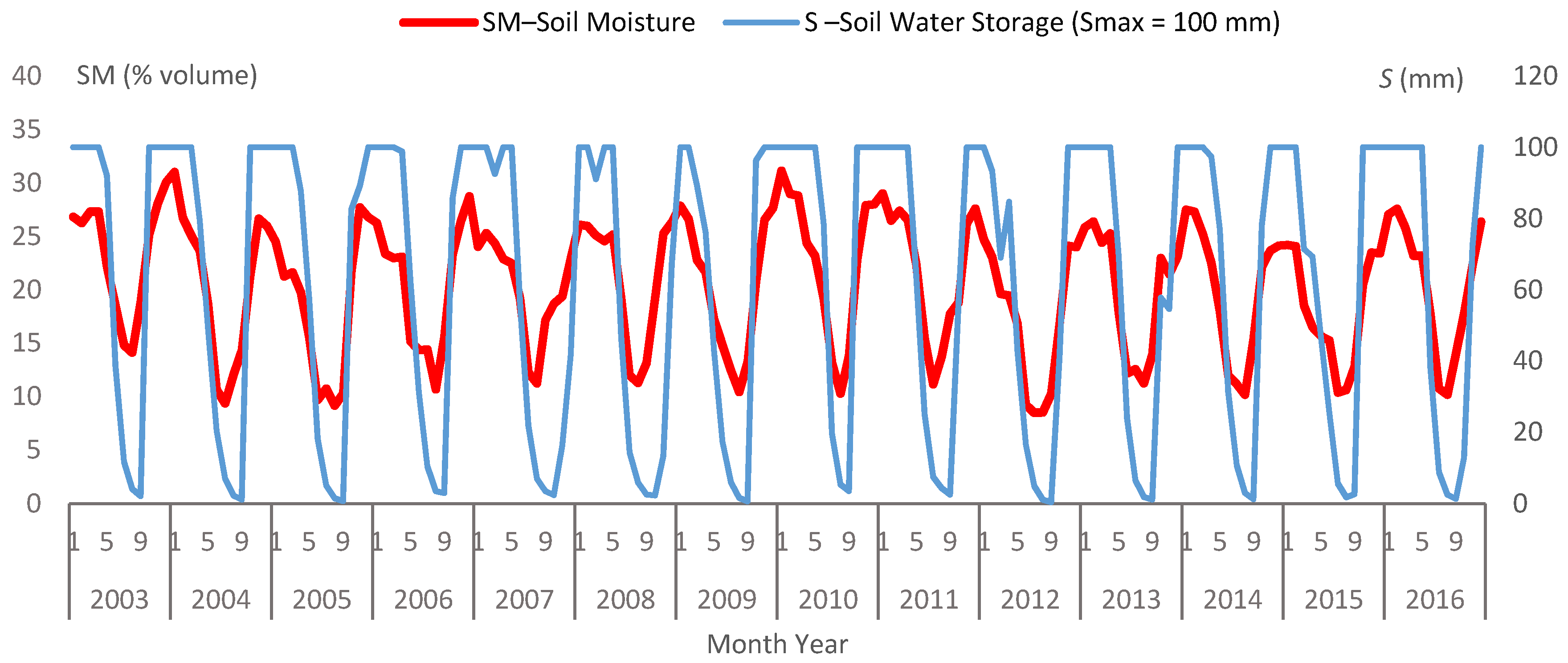
3.1. Soil Water Balance and Soil Moisture during the Study Period

During 14 years, the study period’s annual P and ETo were, on average, 751.3 and 711.4 mm, respectively. The annual ETo ranged from 659.8 mm, in 2017, to 751.5 mm, in 2015. A far higher data dispersion was found for P (Figure 2), with a coefficient of variation (standard deviation/mean) of 0.45, against 0.03 for ETo. The driest of the 14 years was 2012 (P = 359.7 mm), closely followed by 2005 (382.4 mm), which is a figure below the eighth percentile. The largest P record was 1584.6 mm in 2010, an exceptionally high value for Bragança, though not considered a statistical outlier of the annual P series.

The annual values of the soil water balance (SWB) output variables for the study period are also depicted in Figure 2. The average annual ETr, WD and WS were quite similar during the study period (383.7, 327.7 and 367.6 mm, respectively), though with very different data dispersions, with the highest being for WS.

The average monthly SWB in Bragança, which was computed using the P and ETo monthly averages for the study period, reflected the typical Mediterranean pattern prevailing in the study area (Figure 3a). While the periods of soil water deficit (WD) and superavit (WS) were clearly identified, the soil water recharge was hardly noticeable in the September–October months, as the first autumn rainfalls filled the soil storage capacity up to its maximum, generating a superavit from October to April. The water deficit season lasted from May to September, with a peak deficit in July (Figure 3a).

Average annual values of the SWB variables for the study period showed small differences in comparison with the long-term averages, which were positive for WD and WS, negative for ETr and negligibly negative for ETo and P (Figure 3b). The long-term SWB was computed using the last published climatological normal from 1971–2000, namely, with the thirty-year monthly average temperature and precipitation [72]. Their monthly distribution throughout the year was similar in both calculation periods (Figure 3a), though with a higher P in October in the study period than in the 1971–2000 one. Despite the aforementioned differences, the study period was assumed to provide an adequate representation of the normal climatic conditions prevailing in the case study area.

During the study period, the extent of the dry season (number of months) and annual WD (mm) were positively correlated (r = 0.725). A large range in the dry season extent occurred throughout the series, with the dry season lasting from 4 to 9 months with a median duration of 7 months (Figure 4). The annual WD was more dependent on the starting than on the ending month of the dry season. The longest and the shortest recorded wet seasons lasted for 8 and 3 months, respectively, and a very strong correlation was found between the WS and P annual values (r = 0.983).

The monthly SM ranged from 0.085 to 0.311 m³/m³, while the monthly averages computed for the study period were the lowest in August (SM = 0.110) and the highest in January (SM = 0.269). The lowest annual SM average was found in 2012 (SM = 0.171), the year with the lowest P in the series. The average annual SM was negatively correlated with the extent of the dry season (r = −0.843).

3.2. Relationship between the Soil Water Storage and the Satellite-Borne Soil Moisture Data

The overlap for the study period of the monthly ground SWB data (soil water storage, S) and satellite-borne data (SM as a volume percentage) is shown in Figure 5. Close matching of the two series was found for this case study and the data exploration proceeded to regression analysis. Indeed, the wet and dry seasons, as well as the soil water recharge and depletion periods, were clearly identified. However, the SM kept varying in the wetter months, while S flattened at Smax (100 mm in the Figure 5 example).

The model performance indicators (r², CE, RMSE and SEE), together with the parameters of the regression equations relating soil water storage (S, based on the ground data) with the soil moisture (SM, satellite-borne data) are presented in

Table 2. Regression parameters and performance indicators for models I and II that were applied with different soil water storage capacities, Smax (SM, %, independent variable; S, mm, dependent variable; n = 168).

Model	Parameter	Smax (mm)
		25	50	75	100	150
	b	1.69	3.31	4.75	5.98	7.79
	a	−20.04	−37.25	−50.49	−58.88	−61.42
(I)	r2	0.826	0.846	0.837	0.809	0.732
Linear bounded	CE	0.814	0.837	0.831	0.805	0.731
0 < S < Smax	RMSE (mm)	5.017	9.056	13.293	18.185	29.100
	SEE (mm)	3.909	7.281	10.993	15.235	24.065
	SEE (%Smax)	16%	15%	15%	15%	16%
	b	−1.15	−0.80	−0.69	−0.63	−0.54
	a	24.50	15.17	12.11	10.48	8.52
(II)	r2	0.830	0.886	0.845	0.793	0.690
Logistic	CE	0.810	0.884	0.833	0.766	0.624
	RMSE (mm)	5.076	7.641	13.205	19.944	34.398
	SEE (mm)	4.778	7.454	12.387	18.299	30.986
	SEE (%Smax)	19%	15%	17%	18%	21%

r²: determination coefficient, CE: efficiency coefficient, RMSE: root mean square error, SEE: standard error of the estimate.

. The tested models, described in the Materials and Methods section, were linear bounded (I) and logistic (II). These were applied for Smax ranging from very low (25 mm) to high (150 mm). Figure 6 depicts an example of models’ fits to the data for Smax 50 mm.

The determination coefficients (r²) ranged from 0.690 (model II, logistic, with Smax 150 mm) to 0.886 (model II, logistic, with Smax 50 mm), meaning a minimum correlation coefficient (r) of 0.831 when all models and Smax’s were considered. For the range of Smax’s tested, the maximum r² was reached with 50 mm for both models (Figure 7a). Model II showed a higher r² than model I for Smax 25 to 75 mm, and a lower r² for the higher Smax’s (100 and 150 mm). A similar model performance pattern of change was found for CE, with values slightly lower than r². RMSE ranged similarly in both models from 5 mm (Smax 25 mm) to 29 and 34 mm (Smax 150 mm) in models I and II, respectively. A similar increase with the Smax increase was also found for SEE, though with lower values and more pronounced differences between the models (4–24 mm in model I and 5–31 mm in model II in the Smax range 25–150 mm). When expressed as a proportion of Smax, SEE fell into a much narrower range in model I (15–16%) and model II (15–21%, with 18% as the median) (Figure 7b).

In both models, the b regression parameters increased with the Smax increase, while the opposite occurred with the a parameters; these changes expressed the effect of the S scale in its relationship with SM. The best-fitting functions relating a and b with Smax were obtained for both models with the following results:

Model I—Linear bounded

$$b = 0.822 + 0.049\mathrm{Smax}, r^2 = 0.982,$$

(3)

$$a = -19.628 - 0.325\mathrm{Smax}, r^2= 0.832.$$

(4)

Model II—Logistic

$$b = 4{.260\mathrm{Smax}}^{-0.417}, r^2= 0.989,$$

(5)

$$a = 157{.290\mathrm{Smax}}^{-0.585}, r^2 = 0.994.$$

(6)

In all four cases, the correlation with Smax was statistically significant and, except for the model I a parameter (Equation (4)), the r² of the regression functions were very high. As expected, non-linear functions of Smax best fit the a and b parameters of the logistic model. The above equations allow for estimates of the S vs. SM regression parameters for any Smax, therefore providing, for each model, a single relationship S vs. SM that simultaneously accounts for Smax in an S estimation, as follows:

Model I—Linear bounded

$$S^{*}= -19.628 - 0.325\mathrm{Smax} + 0.822\mathrm{SM} + 0.049\mathrm{Smax} \times \mathrm{SM}, r^2 = 0.856, \mathrm{CE} = 0.856.$$

(7)

Model II—Logistic

$$S^{*}=\frac{\mathrm{Smax}}{{1+\mathrm{e}}^{\left(157{.290\mathrm{Smax}}^{-0.588}- 4{.260\mathrm{Smax}}^{-0.417}\mathrm{SM}\right)}}, r^2 = 0.856, \mathrm{CE} = 0.834.$$

(8)

As shown in Figure 6 for Smax 50 mm, the logistic model (II) provided a visibly more adequate representation of the relationship between S and SM compared with the linear model (I). However, the linear model overcame the logistic model’s performance (measured using r² and CE) for larger Smax’s, depicting a lower SEE for all Smax’s (Figure 7). In the models given above with two variables (SM and Smax; Equations (7) and (8)), the linear and the logistic models had similar performances (as measured using r²) in the whole range of Smax, although the linear model showed a slightly higher CE compared to the logistic model. It should be noted that Equations (7) and (8) describe the prediction surfaces of S responding to the SM and Smax input data, as calibrated for the Bragança area, which performed better in the first case but was better represented in the second one.

3.3. Soil Water Depletion and Recharge Phases

As stressed earlier, in a large number of wet months, from late autumn to early spring, Smax was reached, meaning a constant S value, while SM was not constant in those months. On the other hand, the soil water recharge during early autumn was much faster than the depletion during spring. This evidence encouraged deeper analysis of the S vs. SM coupled data series, with the regression analysis for each year of the study period and a chronological plot of the relationship SM vs. S shown in Figure 8.

Taking Smax 100 mm as an example, the quality of the relationship varied sharply throughout the study period, with r² ranging from 0.532 and 0.960 for the linear model and from 0.414 to 0.945 in the logistic model. Keeping Smax 100 mm as an example, Figure 8 depicts the large differences between years of the study period in terms of the monthly chronological changes of SM and S, with the four years depicted being ranked from low to high r² of the relationship. A large part of the recharge (wetting) and depletion (drying) phases presented a distinct S for the similar SM and vice versa. This was increasingly more evident as r² decreased, with clockwise progress from January to December being visible in 2008, where r² was as low as 0.600. As such, the model performance for the whole study period was seemingly affected by the different shape of the S vs. SM relationship in the soil water recharge and depletion phases. Following this, the previous data analysis steps were performed separately for the two data subsets in which the original series was segregated: soil water recharge months and depletion months.

Table 3. Regression parameters and performance indicators of the logistic model applied to the segregated data series with different soil water storage capacities, Smax: segregated model (III) considering the drying and wetting subsets independently and merged (SM, %, independent variable; S, mm, dependent variable).

Model	Parameter	Smax (mm)
		25	50	75	100	150
	b	−1.05	−0.74	−0.65	−0.60	−0.56
(III)	a	21.53	13.42	10.76	9.43	8.01
Segregated	r2	0.867	0.875	0.864	0.846	0.830
Drying	CE	0.883	0.892	0.878	0.856	0.848
Curve	RMSE (mm)	3.878	7.078	10.750	14.648	20.161
(n = 91)	SEE (mm)	4.409	5.974	8.994	13.421	20.460
	SEE (%Smax)	18%	12%	12%	13%	14%
	b	−1.37	−0.93	−0.79	−0.71	−0.60
(III)	a	30.70	18.61	14.86	12.97	10.64
Segregated	r2	0.730	0.770	0.781	0.765	0.673
Wetting	CE	0.543	0.851	0.849	0.788	0.640
Curve	RMSE (mm)	7.677	8.839	13.208	20.279	36.227
(n = 77)	SEE (mm)	4.607	7.599	10.558	13.738	19.151
	SEE (%Smax)	18%	15%	14%	14%	13%
(III)	r2	0.836	0.892	0.886	0.869	0.834
Segregated	CE	0.740	0.875	0.864	0.820	0.739
Drying + Wetting	RMSE (mm)	5.930	7.934	11.940	17.455	28.665
(n = 168)	SEE (mm)	4.702	7.261	10.671	14.646	22.989
	SEE (%Smax)	19%	15%	14%	15%	15%

shows the results of the segregated model (III) applied to the drying curve, wetting curve and drying + wetting curve. For each series and maximum storage tested, the drying curves presented a higher r² than the wetting curves, with SEE varying in the opposite way. The drying curve was fitted to a larger data set, 91 out of 168 months, while the wetting curve was fitted to the remaining 77 months. For the drying curves, r² ranged from 0.810 (Smax 150 mm) to 0.875 (Smax 50 mm), and the same trend was observed for CE. For the wetting curves, the best r² was obtained at Smax 75 (0.781), while a higher CE was associated with Smax 50 mm. For both curves and the drying + wetting curves, RMSE and SEE showed the same patterns found in models I and II, with both increasing as Smax increased. Furthermore, the percentage of SEE in Smax ranged from 12 to 18% (drying curve), 13 to 18% (wetting curve) and 14 to 19% (drying + wetting curve). Compared to the logistic approach applied to all data (model II, Table 2), data segregation in the drying and wetting periods (model III, Table 3) produced better global predictability of S from SM, presenting a higher r² and a lower SEE for each Smax tested (Figure 9). Improvements in the model’s performance were more pronounced in larger Smax (from 75 to 150 mm), where segregation of the data series was visibly more effective in increasing r² and lowering SEE. Smax 50 mm remained the best-performing soil water storage capacity (r² = 0.892 in model III against r² = 0.886 in model II); Figure 10 depicts model III fitted to S vs. SM data with Smax 50 mm.

Following the approach applied to models I and II, Equations (7) and (8) allow for S estimations from SM and Smax, considering the a and b parameters shown in Table 2. The r²’s of the non-linear relationships between the model regression parameters and Smax were all very high. In fact, for the drying curve a and b parameters, r² was 0.986 and 0.957, respectively; for the wetting curve a and b parameters, r² was 0.989 and 0.991, respectively.

Model III—Segregated drying and wetting curve

$$S_{\mathit{drying}}^{*}=\frac{\mathrm{Smax}}{{1+\mathrm{e}}^{\left(122{.86\mathrm{Smax}}^{-0.555 }- 3{.1199\mathrm{Smax}}^{-0.354}\mathrm{SM}\right) }}, r^2 = 0.831, \mathrm{CE} = 0.799,$$

(9)

$$S_{\mathit{wetting}}^{*}=\frac{\mathrm{Smax}}{{1+\mathrm{e}}^{(196{.3\mathrm{Smax}}^{-0.59 }- 5{.7703\mathrm{Smax}}^{-0.456}\mathrm{SM})}}, r^2 = 0.973, \mathrm{CE} = 0.926.$$

(10)

The combined application of the two above equations (Equations (9) and (10)) with the respective data subsets produced the global response (drying + wetting) of model III, with r² = 0.887 and CE = 0.868. Compared to the results obtained using Equation (8), the segregated two-variable logistic model that was used to account for soil water recharge and depletion periods showed better performance for the whole range of Smax tested, reaching a higher r² and CE. Again, these results highlight the effect of segregating data series in the wetting and drying subsets in improving the model’s performance and predictive capacity in the estimation of S from SM.

3.4. Outliers’ Effect on the Model Performance

The results presented correspond to an unscreened series of SM and S data. Yet, from the 168 monthly values, a small number fell far from the general trend defining the relationship between S and SM. No plausible explanation for such deviations was devised and; therefore, a screening exercise for identifying outliers was carried out.

As a first approach, the standardised residuals (SRs) of the trend lines fitted to S vs. SM data (for each one of the Smax tested) were used to screen outliers [90]. This approach implies defining an SR threshold as a screening criterion, which is a user-dependent decision that is supported by experience, expert assistance or the literature [89]. Absolute values of the standardised residuals (ABS SRs) of 3.0, 2.5 and 2.0 were adopted in the exercise, although no guiding values exist for this case. For ABS SR > 3.0, 2 outliers were detected, for ABS SR > 2.5, 7 outliers were detected, and for ABS SR > 2.0, 16 outliers were detected.

In a second approach, the interquartile range rule (IQR) [91] was applied to the residuals of the trend line fitted to S vs. SM data (for each one of the Smax tested). Residuals falling out of the range defined by the following limits corresponded to outliers in the relationship between S and SM (Q₁ and Q₃ are the first and third quartiles of the residuals’ series):

Outlier < Q₁ − 1.5(Q₃ − Q₁) or Outlier > Q₃ + 1.5(Q₃ − Q₁).

(11)

Eight outliers were detected using these rules. As a criterion that is not user-dependent, it was preferred to the ABS SR threshold approach. The performance of the regression models was tested using the data series after the outliers identified using the IQR were discarded (n = 160 for each Smax;

Table 4. Regression parameters and performance indicators of models I, II and III, which were applied with different soil water storage capacities, Smax: outlier-removed data series obtained using the interquartile range rule (SM, %, independent variable; S, mm, dependent variable; n = 160).

Model	Parameter	Smax (mm)
		25	50	75	100	150
	b	1.70	3.33	4.78	6.02	7.83
	a	−20.03	−37.15	−49.84	−57.62	−59.05
(I)	r2	0.870	0.901	0.894	0.872	0.798
Linear bounded	CE	0.857	0.889	0.885	0.865	0.795
0 < S < Smax	RMSE (mm)	4.39	7.433	10.93	15.009	24.982
	SEE (mm)	3.446	5.966	9.029	12.666	21.163
	SEE (%Smax)	14%	12%	12%	13%	14%
	b	−1.15	−0.81	−0.69	−0.63	−0.55
	a	24.26	15.04	11.95	10.33	8.38
(II)	r2	0.886	0.943	0.912	0.874	0.783
Logistic	CE	0.875	0.942	0.906	0.86	0.743
	RMSE (mm)	4.113	5.383	9.881	15.257	27.972
	SEE (mm)	3.923	5.341	9.465	14.357	25.928
	SEE (%Smax)	16%	11%	13%	14%	17%
	b	−1.05	−0.75	−0.65	−0.61	−0.59
(III)	a	21.49	13.47	10.84	9.53	8.83
Segregated	r2	0.887	0.904	0.897	0.890	0.815
drying	CE	0.881	0.892	0.878	0.868	0.785
curve	RMSE (mm)	3.900	7.074	10.747	14.099	26.175
	SEE (mm)	4.420	5.981	8.995	13.526	18.826
	SEE (%Smax)	18%	12%	12%	14%	13%
	b	−1.37	−0.93	−0.78	−0.70	−0.58
(III)	a	30.26	18.19	14.27	12.41	9.56
Segregated	r2	0.762	0.979	0.949	0.902	0.649
wetting	CE	0.686	0.977	0.947	0.89	0.569
curve	RMSE (mm)	6.195	3.352	7.660	14.290	31.208
	SEE (mm)	4.030	7.337	11.062	14.324	19.020
	SEE (%Smax)	16%	15%	15%	14%	13%
(III)	r2	0.827	0.935	0.920	0.895	0.776
Segregated	CE	0.812	0.934	0.912	0.879	0.733
drying + wetting	RMSE (mm)	5.035	5.750	9.520	14.183	28.379
curve	SEE (mm)	4.333	6.899	10.637	14.715	20.307
	SEE (%Smax)	17%	14%	14%	15%	14%

). Furthermore, the IQR provided guidance for defining the ABS SR threshold value when the first approach was applied (in this case, the ABS SR was approximately 2.5).

The models’ performances visibly improved after the outliers were removed from the data series, as r² ranged from 0.846 to 0.901 in the linear model and from 0.886 to 0.943 in the logistic model (compare with Table 1). Comparing Table 1 and Table 2, the same pattern of change was observed for CE, while a decrease was found for RMSE and SEE, even though the SEE decrease was too small to determine changes when expressed as a proportion of Smax. In contrast, the model parameters did not visibly change when comparing results coming from the original data series with those obtained with the outlier-removed data series. This means the outliers’ removal produced an increase in the models’ performances without a visible change in the equations’ parameters.

These findings are confirmed in Figure 11, where r², SEE (in % of Smax) and the a and b parameters of the regression functions for the original (independent variable) are plotted against those obtained with the outlier-removed data series (dependent variable). The slopes of the trend lines fitted to plotted data, with a null intercept, ranged from 0.904 (SEE, %Smax) to 1.061 (r²), while for the a and b regression parameters, the trend line slopes were 0.975 and 1.005, respectively. The outlier removal increased the global r² by 6%, while for the global SEE, a decrease of ≈10% was observed. For all the models and storage capacities analysed, the removal of outliers did not substantially change the regression equations’ parameters (a decreased by 2.5% and b increased by 0.5%). Furthermore, a and b presented the strongest r²’s, with 0.9997 (a) and 0.99998 (b).

This is an important practical finding as it shows the robustness of the SM vs. S relationship, which was not sensitive to the presence of outliers in the data set; therefore, saving screening procedures prior to the model application. These findings also open the possibility of reducing the dataset to a minimum number of data necessary for model calibration. Thus, the equations obtained using the original data can be taken as a reference for prediction purposes. On the other hand, the model performance indicators (r² and CE, obtained using the outlier-removed data series) can be taken as a reference since the withdrawn data represent uncommon and unexplainable records that are meaningless for defining the relationship between SM and S.

4. Discussion

4.1. Model Comparison

The models describing the relationship between S and SM performed well, showing fairly high-quality standards (r² > 0.8 and CE > 0.8, all models and Smax accounted for). However, the high r² values that were obtained do not entirely describe the models’ performances as large SEE and RMSE values were also found. Rather than compromising the models’ descriptive capabilities, these results should be outlined as a limitation for model prediction purposes. Even though outlier removal led to a decrease in SEE, as indicated above, the reduction was about 10% globally, which is an improvement compared to the original series but too low of a gain in terms of model predictive power.

Dorigo et al. [43] compared the ESA CCI SM combined product with in-situ-based soil moisture observations recorded by the validation ground stations network. The median of the correlation coefficients obtained in each station for the latest merging period (July 2012 to December 2014) was 0.89, varying from 0.96 to 0.79 in the interquartile range (third and first quartiles of the series of correlation coefficients obtained in each station). These r values correspond to r²’s of 0.79, 0.92 and 0.63, respectively. The model performance results in the present study fell in the third to second quartile ranges of r² values obtained in the network of stations where ground soil moisture data validated the SM combined product data [43].

Hydrological and land surface models predicting soil moisture and total soil water storage (TWS) achieved lower performances [60,61]. Tian et al. [60] tested data assimilation effects on the water balance model response, which was performed with soil moisture derived from SMOS and total water storage derived from GRACE. Data assimilation from these sources improved the model surface SM estimates when compared with in situ SM measurements, jointly performing better than the single assimilation (r = 0.47–0.86). A similar approach using a land surface model resulted in improved model estimates, which were matched with in situ measurements, of the surface SM (r = 0.86) and TWS (r = 0.95) [61]. In both studies, no direct relationship between remote and ground SM was provided.

The logistic model generally performed better than the linear model. However, the differences in r² for the logistic model compared to the linear model were small and, for the larger Smax, the latter performed better than the former. As such, in the case of constraints in the calculated means, the linear function can be adopted to convert SM into S with a minimal loss of predictive power. Apart from its practical simplicity, the linear model showed equally practical constraints, as it was necessarily bounded by upper (S = Smax) and lower limits (S = 0), meaning that the linear function only applies to the 0 to Smax range. This actually means that for SM < −a/b and SM > (Smax − a)/b, S is not predicted by the linear function but is kept constant and equal to 0 or Smax, respectively (a (intercept) and b (slope) are the linear regression parameters). Therefore, the linear model coupled three functions within the range of SM, with the thresholds for shifting from one to the other being variable with Smax.

In contrast, with the logistic model, a single function enabled describing the S vs. SM relationship for the whole range of SM, which is a practical advantage for calculation routines. Furthermore, the approach to S = 0 and S = Smax is asymptotical, meaning that, although the residuals of the regression line are higher in the logistic model compared to the linear model for the range of SM in which S = Smax and S = 0, the opposite occurs for the data not strictly matching this condition. In fact, high SM values not matching S = Smax or S = Smax values not matching high SM values generate lower the residuals of the regression line in the logistic model compared to the linear model, mutatis mutandis for the S = 0 range of SM data (see Figure 6). This seemingly contributed to explaining the better performance of the logistic model for most of the Smax values tested compared to that of the linear model. Furthermore, as shown in the example presented in Figure 6, the logistic model apparently fit the data better within the range 0 < S < Smax, and within this range, the logistic function depicted a quasi-linear shape.

Furthermore, the logistic model seemingly better represented S’s behaviour in its lower range. In fact, the Thornthwaite–Mather method [83] applied in this study for computing the water balance uses an asymptotical approach to soil water depletion during the drying periods, which rarely results in null values of soil water storage. The linear model cannot represent this behaviour. Apart from the non-linearity in S, non-linearity was also reported in the SM remote appraisal. For instance, non-linearity was observed in the relationship between the in situ soil moisture measurements and the soil dielectric constant for low soil water contents, while for most of its range of application, the relationship was linear [69].

It should be noted that the shape of the S vs. SM relationship is not physically defined yet, meaning that only empirical interpretations can be derived in favour of the non-linearity. Nevertheless, and for the same reason, recommendations for using one of the models and discarding the other can only stand on their performance, assessed on a statistical basis. All in all, the logistic model better described the relationship between S and SM and, globally, was better fitted to data than the linear model in this case study, despite its poorer predictive capabilities, as represented by the large SEE.

4.2. Effect of Smax

The models were applied with the series of S monthly values obtained from the SWB computations using Smax 25 to 150 mm. The models’ performances changed non-monotonically with Smax, as higher r² and CE were obtained for Smax 50 and 75 mm when applying the logistic and linear models, respectively. The model performance indicators decreased either towards the lowest Smax tested or towards the highest one, where the poorest performances were obtained in both the linear and logistic models.

Smax depends on (i) the soil physical characteristics determining the maximum amount of water retained in soil pores that can be extracted by plant roots, and on (ii) the soil depth that is explored by plant roots [84]. The former includes the available water capacity (AWC) and bulk density (BD), with their effect requiring a correction for the presence of coarse particles (>2 mm) in case they were determined in fine soil earth (<2 mm). AWC and BD vary inversely with soil properties, such as texture and organic matter content (SOM). Hence, the product of AWC and BD depicts a narrow range of variation due to soil texture and SOM compared to the much wider range of variation that is associated with the soil depth. This means that Smax depends much more on the defined soil depth than on differences between soil types in terms of what concerns their water retention characteristics.

Despite the wide set of soil types found in the study area, with essential differences in AWC and BD, which are mainly associated with the parent material [79], the Smax per unit soil depth (mm cm⁻¹) ranged from 0.12–0.20 (calculations based on data from [71]). Accordingly, for the Smax tested in this study, the soil depths ranged from 20 cm to 1 m.

The models’ performances were expected to decrease with Smax. In fact, radar penetration does not exceed a 5 cm soil top layer [22]. SM’s sensitivity to maximum storage capacity has already been reported, although not fully assessed for many soil types [62]. Soil water storage, S, is assumed to correspond to a constant moisture value throughout the soil profile. Although this is a reliable assumption for small soil depths, this might not represent the prevailing ground conditions for larger soil depths well. In the latter case, surface soil moisture, represented by SM, may shift from the profile-averaged soil moisture represented by S. Furthermore, this shifting may differ according to the soil wetting or drying phase during the year. Therefore, increasing the soil depth considered as a reference for soil water balance computations may result in a lower model performance, which was actually found in this study.

The decline in model performance for the lower Smax tested does not fit in the above elaboration. An Smax as low as 25 mm resulted in a fast filling of soil water storage capacity during recharge by excess precipitation over the reference evapotranspiration. If Smax is surpassed, the SWB computes the surpassed amount as water superavit. As expected, in this study the mean annual superavit steadily decreased from Smax 25 to 150 mm (438 against 334 mm), as well as the mean annual number of months with superavit in the study period (6 against 4.5 months), which was equal to the number of months with S = Smax. Accordingly, in these months, S remained constant while SM varied at its higher range of values, reflecting water surplus accumulation over the ground surface. This may contribute to explaining the lower quality fit of both models to the data for the lowest Smax tested (25 mm).

4.3. Soil Water Recharge and Depletion

As shown, the segregation of the soil water recharge (wetting) from the depletion (drying) in the data series improved the logistic model’s global performance. Similar S values were estimated from higher SM values in the wetting phase model than those estimated with the drying phase model. This finding is a reminder of the issue of moisture distribution in the soil profile, which is assumed uniform in S. SM reflects soil moisture at its shallow surface layer, which might not correspond to the profile-averaged moisture reflected by S. During the wetting phase in the study area, occurring during autumn and winter, the surface was exposed to frequent rainfalls, regardless of the redistribution rate of infiltrated water within the profile. In contrast, in the drying phase, corresponding to the Mediterranean spring and summer, the surface was exposed to very infrequent rainfalls and high evapotranspiration rates, while the soil storage in the profile declined at a much slower rate than that of water depletion as vapour transfers to the lower atmosphere via the surface soil layer.

The logistic model gave a good representation of this interpretation as an S estimate with the wetting and the drying functions fitted to the data for high and low SM values. The former corresponded to the full profile soil moistening after some months of excess rainfall over the evapotranspiration, while the latter corresponded to the end of the dry season (summer) after a large period of low rainfall amounts and high evapotranspiration rates. The segregation procedure of the two sets of data (wetting and drying phases) was not actually applied for the linear model. In fact, this would result in a non-realistic range of SM values that would produce a constant S estimation at S = 0 and at S = Smax.

The above description represents the hysteretic behaviour of the relationship between SM and S, which is not reported in the literature. In fact, regardless of the source of ground data used to be matched with the satellite-borne data, research has been targeted towards finding a single relationship between both data sets. However, hysteresis has been known for a long time in soil physics and soil hydrology and associated with water flowing through porous media [68,92]. Furthermore, hysteresis is found in surface hydrology, where sediment transport studies in streams show that sediment yields may depict such behaviour, as well as ionic species dissolved or adsorbed to the soiled phase [64,93,94].

4.4. A Note on the Models’ Applicability

The methodological approach followed in this study was strictly statistical, prospecting direct applications in the agricultural water management field. For the case study presented, the approach aimed at converting a remote non-invasive monitoring soil moisture dataset into an actual volume of water in the soil per unit area, according to a specified soil water storage capacity. This is understood as a managerial improvement in this field. The regression functions obtained are the tools being provided to the potential end-users of these research results. The derived two-variable functions are especially highlighted in this context. As such, the expected context of the models’ applications is practical and unsophisticated. Still, care is required in the models’ applications for prediction purposes, given the wide range of possible results that the models’ SEEs demonstrate.

The research reported on a case study located in NE Portugal, NW Iberian Peninsula. As such, the results obtained can be reliably used in applications in this region, not only for agricultural water management purposes but also for other purposes, including drought monitoring, which is an important issue in Mediterranean agri-environments. The ESA CCI SM combined product is developed on the basis of a worldwide network of ground stations providing in situ soil moisture data for the product’s calibration [43]. Local ground data are, therefore, always necessary for improving the product’s performance and local studies may add valuable information to that of the reference network of ground stations feeding SM calibration runs. It is important to stress that the central and north-western part of the Iberian Peninsula is covered by a single reference ground station of the SM calibration network [43]. On one hand, enlarging the SM product spatial coverage with increasing performance is a continuous challenge to which the present case study is intended to contribute. On the other hand, taking into account the spatial coverage of the calibration network of ground stations in the region, the present study’s results can be considered for application in the NW Iberian Peninsula.

The present research applied meteorological data to derive soil water storage from soil water balance computations. As it is consistently related to SM combined product data, soil water storage is shown to have the potential for in situ SM calibration exercises, which was done indirectly in this case. This is a far-reaching prospect for the application of the approach tested in the present case study. In fact, the weather station networks are much larger and have a much denser spatial coverage than that of in situ soil moisture. The a priori definition of Smax for computing the water balance, as demonstrated, is a core element in the prospected developments of the present case study.

5. Conclusions

The ESA SM satellite product provides a remote and large-scale assessment of ground soil moisture at a daily time step. The product is a very interesting tool to be further explored in view of its wider applications in support of a range of research fields, as well as in support of environmental and economic sectors requiring such freely available information. For this, SM validation with ground data has to progress by increasing the number of ground stations and point datasets for comparison purposes to improve the reliability and coverage. Case studies exploring the relationship of SM data with point ground data contribute to such a purpose that the present case study entirely aligns with.

On the other hand, applications of SM data have seemingly not yet achieved the level of demand by end users that such a powerful product is expected to stimulate. The research that is focused on translating SM data to data that is useful and directly usable by the potential end users in several application sectors is still progressing, a research line for which the present study is also intended to contribute towards. Machine learning approaches to better define the relationship between S and SM to provide a more robust predictive tool compared to the conventional statistical methods used in this study is certainly a challenge to be undertaken in future research. As for the present, this study aimed at exploring the relationship between SM and soil water storage, as assessed through the soil water balance computation. In this context, it is worth noting that while SM expresses a remotely assessed volumetric soil water content, the soil water balance is expressed in terms of an equivalent water height in the soil, meaning a volume of water in the soil per unit ground area. This scientifically meaningless difference is, however, a significant asset when it comes to its application by end users.

A major conclusion of the research carried out is that the regression models representing the relationship between S and SM showed fairly high performances, with r² in the range of 0.8 to 0.9. This is an encouraging result in what concerns the use of strictly statistical approaches to deriving prediction tools for soil water storage from satellite-borne soil moisture data, namely the ESA SM product. However, as this study showed, the predictability was limited by the large data scatter around the fitted functions, as indicated by an SEE around 15% of the soil water storage capacity, which represents a still too large standard error when expressed in absolute terms (for instance, 15 mm or more SEE for Smax 100 mm).

A second major conclusion of the research was that the S vs. SM relationship was not unique, where more similar S’s were found for larger SM values when the soil was recharging (wetting phase) than when the soil was depleting water (drying phase). This actually represents a hysteresis in the S vs. SM relationship, which had not been reported earlier; this opens the challenging possibilities for improving the tools used to predict S from SM in a way that accounts for the pattern of evolution of the soil water balance variables along the year. The issue is remarkably important in the Mediterranean climate type, where the long dry season leads to non-uniform topsoil moisture profiles, which is meaningless for the water balance computations but biases SM due to the low penetration depth of satellite radar sensors.

Third, as an important outcome of the research, the parameters of the regression functions, which were obtained for each one of the soil water storage capacity tested, were highly correlated with Smax. Therefore, two-variable models (linear, logistic and segregated) were derived, which represented the soil water storage prediction surface in response to temporally variable SM and spatially variable Smax. Considering the extent of the study period and the level of performance reached (with an r² around 0.85), these models are assumed to be calibrated and, hence, available for validation exercises and use in the Bragança area.

References

1. Bojinski, S.; Verstraete, M.; Peterson, T.C.; Richter, C.; Simmons, A.; Zemp, M. The Concept of Essential Climate Variables in Support of Climate Research, Applications, and Policy. Bull. Am. Meteorol. Soc. 2014, 95, 1431–1443. [Google Scholar] [CrossRef]
2. World Meteorological Organization (WMO), United Nations Educational Scientific and Cultural Organization, United Nations Environment Programme, and International Council for Science. GCOS, 154. Systematic observation requirements for satellite-based data products for climate Supplemental details to the satellite-based component of the Implementation Plan for the Global Observing System for Climate in Support of the UNFCCC (2011 Update). Geneva, Switzerland. 2011. Available online: https://library.wmo.int/index.php?lvl=notice_display&id=12907#.X-jHy9j7TIU (accessed on 10 October 2020).
3. Perkins, S.E.; Argüeso, D.; White, C.J. Relationships between climate variability, soil moisture, and Australian heatwaves. J. Geophys. Res. Atmos. 2015, 120, 8144–8164. [Google Scholar] [CrossRef]
4. Jung, M.; Reichstein, M.; Ciais, P.; Seneviratne, S.I.; Sheffield, J.; Goulden, M.L.; Bonan, G.; Cescatti, A.; Chen, J.; De Jeu, R.; et al. Recent decline in the global land evapotranspiration trend due to limited moisture supply. Nature 2010, 467, 951–954. [Google Scholar] [CrossRef] [PubMed]
5. Stephens, C.M.; Johnson, F.M.; Marshall, L.A. Implications of future climate change for event-based hydrologic models. Adv. Water Resour. 2018, 119, 95–110. [Google Scholar] [CrossRef]
6. Seneviratne, S.I.; Corti, T.; Davin, E.L.; Hirschi, M.; Jaeger, E.B.; Lehner, I.; Orlowsky, B.; Teuling, A.J. Investigating soil moisture–climate interactions in a changing climate: A review. Earth Sci. Rev. 2010, 99, 125–161. [Google Scholar] [CrossRef]
7. Saft, M.; Peel, C.M.; Western, A.W.; Zhang, L. Predicting shifts in rainfall-runoff partitioning during multiyear drought: Roles of dry period and catchment characteristics. J. Am. Water Resour. Assoc. 2016, 52, 9290–9305. [Google Scholar] [CrossRef]
8. Gao, W.; Wang, Z.; Huang, G. Spatiotemporal Variability of Actual Evapotranspiration and the Dominant Climatic Factors in the Pearl River Basin, China. Atmosphere 2019, 10, 340. [Google Scholar] [CrossRef] [Green Version]
9. Lee, E.; Kim, S. Wavelet analysis of soil moisture measurements for hillslope hydrological processes. J. Hydrol. 2019, 575, 82–93. [Google Scholar] [CrossRef]
10. Li, T.; Hao, X.; Kang, S. Spatiotemporal Variability of Soil Moisture as Affected by Soil Properties during Irrigation Cycles. Soil Sci. Soc. Am. J. 2014, 78, 598–608. [Google Scholar] [CrossRef]
11. Liao, K.; Lai, X.; Zhou, Z.; Zhu, Q. Applying fractal analysis to detect spatio-temporal variability of soil moisture content on two contrasting land use hillslopes. Catena 2017, 157, 163–172. [Google Scholar] [CrossRef]
12. Zucco, G.; Brocca, L.; Moramarco, T.; Morbidelli, R. Influence of land use on soil moisture spatial–temporal variability and monitoring. J. Hydrol. 2014, 516, 193–199. [Google Scholar] [CrossRef]
13. Han, D.; Zhou, T. Soil water movement in the unsaturated zone of an inland arid region: Mulched drip irrigation experiment. J. Hydrol. 2018, 559, 13–29. [Google Scholar] [CrossRef]
14. Moiwo, J.P.; Tao, F.; Lu, W. Estimating soil moisture storage change using quasi-terrestrial water balance method. Agric. Water Manag. 2011, 102, 25–34. [Google Scholar] [CrossRef]
15. Yinglan, A.; Wang, G.; Liu, T.; Xue, B.; Kuczera, G. Spatial variation of correlations between vertical soil water and evapotranspiration and their controlling factors in a semi-arid region. J. Hydrol. 2019, 574, 53–63. [Google Scholar] [CrossRef]
16. Bao, Z.; Zhang, J.; Wang, G.; Chen, Q.; Guan, T.; Yan, X.; Liu, C.; Liu, J.; Wang, J. The impact of climate variability and land use/cover change on the water balance in the Middle Yellow River Basin, China. J. Hydrol. 2019, 577, 123942. [Google Scholar] [CrossRef]
17. Reichert, J.M.; Rodrigues, M.F.; Peláez, J.J.Z.; Lanza, R.; Minella, J.P.G.; Arnold, J.G.; Cavalcante, R.B.L. Water balance in paired watersheds with eucalyptus and degraded grassland in Pampa biome. Agric. For. Meteorol. 2017, 237–238, 282–295. [Google Scholar] [CrossRef]
18. Moreira, A.A.; Ruhoff, A.L.; Roberti, D.R.; Souza, V.D.A.; Da Rocha, H.R.; De Paiva, R.C.D. Assessment of terrestrial water balance using remote sensing data in South America. J. Hydrol. 2019, 575, 131–147. [Google Scholar] [CrossRef]
19. Zhang, Y.; Pan, M.; Sheffield, J.; Siemann, A.L.; Fisher, C.K.; Liang, M.; Beck, H.; Wanders, N.; MacCracken, R.; Houser, P.R.; et al. A Climate Data Record (CDR) for the global terrestrial water budget: 1984–2010. Hydrol. Earth Syst. Sci. 2018, 22, 241–263. [Google Scholar] [CrossRef] [Green Version]
20. Chawla, I.; Karthikeyan, L.; Mishra, A.K. A review of remote sensing applications for water security: Quantity, quality, and extremes. J. Hydrol. 2020, 585, 124826. [Google Scholar] [CrossRef]
21. Dorigo, W.A.; Xaver, A.; Vreugdenhil, M.; Gruber, A.; Hegyiová, A.; Sanchis-Dufau, A.D.; Zamojski, D.; Cordes, C.; Wagner, W.; Drusch, M. Global Automated Quality Control of In Situ Soil Moisture Data from the International Soil Moisture Network. Vadose Zone J. 2013, 12. [Google Scholar] [CrossRef]
22. Dorigo, W.A.; Wagner, W.; Albergel, C.; Albrecht, F.; Balsamo, G.; Brocca, L.; Chung, D.; Ertl, M.; Forkel, M.; Gruber, A.; et al. ESA CCI Soil Moisture for improved Earth system understanding: State-of-the art and future directions. Remote Sens. Environ. 2017, 203, 185–215. [Google Scholar] [CrossRef]
23. Vereecken, H.; Huisman, J.A.; Pachepsky, Y.; Montzka, C.; Van Der Kruk, J.; Bogena, H.; Weihermuller, L.; Herbst, M.; Martinez, G.; VanderBorght, J.; et al. On the spatio-temporal dynamics of soil moisture at the field scale. J. Hydrol. 2014, 516, 76–96. [Google Scholar] [CrossRef]
24. Wanders, N.; Karssenberg, D.; De Roo, A.; De Jong, S.M.; Bierkens, M.F.P. The suitability of remotely sensed soil moisture for improving operational flood forecasting. Hydrol. Earth Syst. Sci. 2014, 18, 2343–2357. [Google Scholar] [CrossRef] [Green Version]
25. Gruber, A.; Scanlon, T.; Van Der Schalie, R.; Wagner, W.; Dorigo, W. Evolution of the ESA CCI Soil Moisture climate data records and their underlying merging methodology. Earth Syst. Sci. Data 2019, 11, 717–739. [Google Scholar] [CrossRef] [Green Version]
26. Nair, A.S.; Indu, J. Improvement of land surface model simulations over India via data assimilation of satellite-based soil moisture products. J. Hydrol. 2019, 573, 406–421. [Google Scholar] [CrossRef]
27. Mohamed, E.S.; Ali, A.; El-Shirbeny, M.; Abutaleb, K.; Shaddad, S.M. Mapping soil moisture and their correlation with crop pattern using remotely sensed data in arid region. Egypt. J. Remote Sens. Space Sci. 2019. [Google Scholar] [CrossRef]
28. Lai, C.; Zhong, R.; Wang, Z.; Wu, X.; Chen, X.; Wang, P.; Lian, Y. Monitoring hydrological drought using long-term satellite-based precipitation data. Sci. Total Environ. 2019, 649, 1198–1208. [Google Scholar] [CrossRef]
29. Zhao, M.; Geruo, A.; Velicogna, I.; Kimball, J.S. Satellite Observations of Regional Drought Severity in the Continental United States Using GRACE-Based Terrestrial Water Storage Changes. J. Clim. 2017, 30, 6297–6308. [Google Scholar] [CrossRef]
30. Mishra, A.; Vu, T.; Veettil, A.V.; Entekhabi, D. Drought monitoring with soil moisture active passive (SMAP) measurements. J. Hydrol. 2017, 552, 620–632. [Google Scholar] [CrossRef]
31. Park, S.; Im, J.; Park, S.; Rhee, J. Drought monitoring using high resolution soil moisture through multi-sensor satellite data fusion over the Korean peninsula. Agric. For. Meteorol. 2017, 237–238, 257–269. [Google Scholar] [CrossRef]
32. Sanchez, N.; González-Zamora, Á.; Martínez-Fernández, J.; Piles, M.; Pablos, M. Integrated remote sensing approach to global agricultural drought monitoring. Agric. For. Meteorol. 2018, 259, 141–153. [Google Scholar] [CrossRef]
33. Jalilvand, E.; Tajrishy, M.; Ghazi Zadeh Hashemi, S.A.; Brocca, L. Quantification of irrigation water using remote sensing of soil moisture in a semi-arid region. Remote Sens. Environ. 2019, 231, 111226. [Google Scholar] [CrossRef]
34. Wasko, C.; Nathan, R. Influence of changes in rainfall and soil moisture on trends in flooding. J. Hydrol. 2019, 575, 432–441. [Google Scholar] [CrossRef]
35. Asoka, A.; Gleeson, T.; Wada, Y.; Mishra, V. Relative contribution of monsoon precipitation and pumping to changes in groundwater storage in India. Nat. Geosci. 2017, 10, 109–117. [Google Scholar] [CrossRef] [Green Version]
36. Liu, Y.; Liu, Y.; Wang, W. Inter-comparison of satellite-retrieved and Global Land Data Assimilation System-simulated soil moisture datasets for global drought analysis. Remote Sens. Environ. 2019, 220, 1–18. [Google Scholar] [CrossRef]
37. Plummer, S.; LeComte, P.; Doherty, M. The ESA Climate Change Initiative (CCI): A European contribution to the generation of the Global Climate Observing System. Remote Sens. Environ. 2017, 203, 2–8. [Google Scholar] [CrossRef]
38. Pasik, A.; Scanlon, T.; Dorigo, W.; de Jeu, R.A.M.; Hahn, S.; van der Schaile, R.; Wagner, W.; Kidd, R.; Gruber, A.; Moesinger, L.; et al. ESA Climate Change Initiative Plus—Soil Moisture—Algorithm Theoretical Baseline Document (ATBD) D2.1 Supporting Product Version v05.2. 2020. Available online: https://www.esa-soilmoisture-cci.org/sites/default/files/documents/public/CCI%20SM%20v05.2%20documentation/ESA_CCI_SM_RD_D2.1_v1_ATBD_v05.2.pdf (accessed on 1 November 2020).
39. Petropoulos, G.P.; Ireland, G.; Barrett, B. Surface soil moisture retrievals from remote sensing: Current status, products & future trends. Phys. Chem. Earth. 2015, 83–84, 36–56. [Google Scholar] [CrossRef]
40. Chakravorty, A.; Chahar, B.R.; Sharma, O.P.; Dhanya, C.T. A regional scale performance evaluation of SMOS and ESA-CCI soil moisture products over India with simulated soil moisture from MERRA-Land. Remote Sens. Environ. 2016, 186, 514–527. [Google Scholar] [CrossRef]
41. González-Zamora, Á.; Sanchez, N.; Pablos, M.; Martínez-Fernández, J. CCI soil moisture assessment with SMOS soil moisture and in situ data under different environmental conditions and spatial scales in Spain. Remote Sens. Environ. 2019, 225, 469–482. [Google Scholar] [CrossRef]
42. Kovačević, J.; Cvijetinovic, Z.; Stančić, N.; Brodić, N.; Mihajlović, D. New Downscaling Approach Using ESA CCI SM Products for Obtaining High Resolution Surface Soil Moisture. Remote Sens. 2020, 12, 1119. [Google Scholar] [CrossRef] [Green Version]
43. Dorigo, W.A.; Gruber, A.; De Jeu, R.A.M.; Wagner, W.; Stacke, T.; Loew, A.; Albergel, C.; Brocca, L.; Chung, D.; Parinussa, R.M.; et al. Evaluation of the ESA CCI soil moisture product using ground-based observations. Remote Sens. Environ. 2015, 162, 380–395. [Google Scholar] [CrossRef]
44. Martens, B.; Gonzalez Miralles, D.; Lievens, H.; Van Der Schalie, R.; De Jeu, R.A.M.; Fernández-Prieto, D.; Beck, H.E.; Dorigo, W.A.; Verhoest, N. GLEAM v3: Satellite-based land evaporation and root-zone soil moisture. Geosci. Model Dev. 2017, 10, 1903–1925. [Google Scholar] [CrossRef] [Green Version]
45. Pan, N.; Wang, S.; Liu, Y.; Zhao, W.; Fu, B. Global Surface Soil Moisture Dynamics in 1979–2016 Observed from ESA CCI SM Dataset. Water 2019, 11, 883. [Google Scholar] [CrossRef] [Green Version]
46. Nicolai-Shaw, N.; Zscheischler, J.; Hirschi, M.; Gudmundsson, L.; Seneviratne, S.I. A drought event composite analysis using satellite remote-sensing based soil moisture. Remote Sens. Environ. 2017, 203, 216–225. [Google Scholar] [CrossRef]
47. Hirschi, M.; Mueller, B.; Dorigo, W.; Seneviratne, S.I. Using remotely sensed soil moisture for land–atmosphere coupling diagnostics: The role of surface vs. root-zone soil moisture variability. Remote Sens. Environ. 2014, 154, 246–252. [Google Scholar] [CrossRef] [Green Version]
48. Deng, Y.; Wang, S.; Bai, X.; Luo, G.; Wu, L.; Cao, Y.; Li, H.; Li, C.; Yang, Y.; Hu, Z.; et al. Variation trend of global soil moisture and its cause analysis. Ecol. Indic. 2020, 110, 105939. [Google Scholar] [CrossRef]
49. Zohaib, M.; Kim, H.; Choi, M. Detecting global irrigated areas by using satellite and reanalysis products. Sci. Total Environ. 2019, 677, 679–691. [Google Scholar] [CrossRef]
50. Sakai, T.; Iizumi, T.; Okada, M.; Nishimori, M.; Grünwald, T.; Prueger, J.; Cescatti, A.; Korres, W.; Schmidt, M.; Carrara, A.; et al. Varying applicability of four different satellite-derived soil moisture products to global gridded crop model evaluation. Int. J. Appl. Earth Obs. Geoinf. 2016, 48, 51–60. [Google Scholar] [CrossRef]
51. Wang, S.; Mo, X.; Liu, S.; Lin, Z.; Hu, S. Validation and trend analysis of ECV soil moisture data on cropland in North China Plain during 1981–2010. Int. J. Appl. Earth Obs. Geoinf. 2016, 48, 110–121. [Google Scholar] [CrossRef]
52. Abera, W.; Formetta, G.; Brocca, L.; Rigon, R. Modeling the water budget of the Upper Blue Nile basin using the JGrass-NewAge model system and satellite data. Hydrol. Earth Syst. Sci. 2017, 21, 3145–3165. [Google Scholar] [CrossRef] [Green Version]
53. Gao, H.; Tang, Q.H.; Ferguson, C.R.; Wood, E.F.; Lettenmaier, D.P. Estimating the water budget of major US river basins via remote sensing. Int. J. Remote Sens. 2010, 31, 3955–3978. [Google Scholar] [CrossRef]
54. Mohebzadeh, H.; Fallah, M. Quantitative analysis of water balance components in Lake Urmia, Iran using remote sensing technology. Remote Sens. Appl. Soc. Environ. 2019, 13, 389–400. [Google Scholar] [CrossRef]
55. Oliveira, P.T.S.; Nearing, M.A.; Moran, M.S.; Goodrich, D.C.; Wendland, E.; Gupta, H.V. Trends in water balance components across the Brazilian. Water Resour. Res. 2014, 50, 7100–7114. [Google Scholar] [CrossRef] [Green Version]
56. Pan, M.; Sahoo, A.K.; Troy, T.J.; Vinukollu, R.K.; Sheffield, J.; Wood, A.E.F. Multisource Estimation of Long-Term Terrestrial Water Budget for Major Global River Basins. J. Clim. 2012, 25, 3191–3206. [Google Scholar] [CrossRef]
57. Sahoo, A.K.; Pan, M.; Troy, T.J.; Vinukollu, R.K.; Sheffield, J.; Wood, A.E.F. Reconciling the global terrestrial water budget using satellite remote sensing. Remote Sens. Environ. 2011, 115, 1850–1865. [Google Scholar] [CrossRef]
58. Sheffield, J.; Ferguson, C.R.; Troy, T.J.; Wood, E.F.; McCabe, M.F. Closing the terrestrial water budget from satellite remote sensing. Geophys. Res. Lett. 2009, 36, 1–5. [Google Scholar] [CrossRef]
59. Wang, H.; Guan, H.; Gutiérrez-Jurado, H.A.; Simmons, C.T. Examination of water budget using satellite products over Australia. J. Hydrol. 2014, 511, 546–554. [Google Scholar] [CrossRef]
60. Tian, S.; Tregoning, P.; Renzullo, L.J.; Van Dijk, A.I.J.M.; Walker, J.P.; Pauwels, V.R.N.; Allgeyer, S. Improved water balance component estimates through joint assimilation of GRACE water storage and SMOS soil moisture retrievals. Water Resour. Res. 2017, 53, 1820–1840. [Google Scholar] [CrossRef]
61. Girotto, M.; Reichle, R.H.; Rodell, M.; Liu, Q.; Mahanama, S.; De Lannoy, G.J.M. Multi-sensor assimilation of SMOS brightness temperature and GRACE terrestrial water storage observations for soil moisture and shallow groundwater estimation. Remote Sens. Environ. 2019, 227, 12–27. [Google Scholar] [CrossRef]
62. Demirel, M.C.; Özen, A.; Orta, S.; Toker, E.; Demir, H.K.; Ekmekcioğlu, Ö.; Tayşi, H.; Eruçar, S.; Sağ, A.B.; Sari, Ö.; et al. Additional Value of Using Satellite-Based Soil Moisture and Two Sources of Groundwater Data for Hydrological Model Calibration. Water 2019, 11, 2083. [Google Scholar] [CrossRef] [Green Version]
63. Nijzink, R.C.; Almeida, S.; Pechlivanidis, I.; Capell, R.; Gustafssons, D.; Arheimer, B.; Parajka, J.; Freer, J.; Han, D.; Wagener, T.; et al. Constraining Conceptual Hydrological Models with Multiple Information Sources. Water Resour. Res. 2018, 54, 8332–8362. [Google Scholar] [CrossRef] [Green Version]
64. Du, H.; Fok, H.S.; Chen, Y.; Ma, Z. Characterization of the Recharge-Storage-Runoff Process of the Yangtze River Source Region under Climate Change. Water 2020, 12, 1940. [Google Scholar] [CrossRef]
65. Nie, N.; Zhang, W.; Zhang, Z.; Guo, H.; Ishwaran, N. Reconstructed Terrestrial Water Storage Change (ΔTWS) from 1948 to 2012 over the Amazon Basin with the Latest GRACE and GLDAS Products. Water Resour. Manag. 2016, 30, 279–294. [Google Scholar] [CrossRef]
66. Senyurek, V.; Lei, F.; Boyd, D.; Gurbuz, A.C.; Kurum, M.; Moorhead, R. Evaluations of Machine Learning-Based CYGNSS Soil Moisture Estimates against SMAP Observations. Remote Sens. 2020, 12, 3503. [Google Scholar] [CrossRef]
67. Zhuo, L.; Han, D. Could operational hydrological models be made compatible with satellite soil moisture observations? Hydrol. Process. 2016, 30, 1637–1648. [Google Scholar] [CrossRef] [Green Version]
68. Hillel, D. Introduction to Environmental Soil Physics; Elsevier: Amsterdam, The Netherlands, 2003. [Google Scholar]
69. Chanzy, A.; Chadoeuf, J.; Gaudu, J.C.; Mohrath, D.; Richard, G.; Bruckler, L. Soil moisture monitoring at the field scale using automatic capacitance probes. Eur. J. Soil Sci. 1998, 49, 637–648. [Google Scholar] [CrossRef]
70. Köppen, W. Das geograsphica system der Klimate [On a geographic system of climate]. In Handbuch der Klimatologie; Köppen, W., Geiger, G., Eds.; Gebr. Bontraerger: Stuttgart, Germany, 1936; pp. 1–44. [Google Scholar]
71. Agroconsultores & Coba, Carta dos Solos, Carta do Uso Actual e Carta de Aptidão da Terra do Nordeste de Portugal; Universidade de Trás-os-Montes e Alto Douro: Vila Real, Portugal, 1991.
72. Instituto Português do Mar e da Atmosfera (IPMA). Normais Climatológicas 1971–2000. 2019. Available online: https://www.ipma.pt/pt/oclima/normais.clima/1971-2000/ (accessed on 24 September 2019).
73. Cherlet, M.; Hutchinson, C.; Reynolds, J.; Hill, J.; Sommer, S.; von Maltitz, G. World Atlas Desertification, 3rd ed.; Publication Office of the European Union: Luxembourg, 2018. [Google Scholar]
74. PANCD, Programa de Acção Nacional de Combate à Desertificação, Revisão 2011/2020; Ponto Focal Nacional da Comissão das Nações Unidas de Combate à Desertificação: Lisboa, Portugal. 2011. Available online: http://www2.icnf.pt/portal/pn/biodiversidade/ei/unccd-PT/resource/doc/pandc/2011-2020-rel-fact-criticos.pdf (accessed on 1 November 2020).
75. de Figueiredo, T.; Fonseca, F.; Nunes, L. (Eds.) Os solos e a suscetibilidade à desertificação no NE de Portugal. In Proteção do Solo e Combate à Desertificação: Oportunidade Para as Regiões Transfronteiriças; Instituto Politécnico de Bragança: Bragança, Portugal, 2015; pp. 87–100. [Google Scholar]
76. de Figueiredo, T.; Fonseca, F.; Pinheiro, H. Fire hazard and susceptibility to desertification: A territorial approach in NE Portugal. In Multidimensão e Territórios de Risco; I. da U. de Coimbra and P. e S. RISCOS—Associação Portuguesa de Riscos: Coimbra, Portugal, 2014; pp. 117–121. [Google Scholar]
77. Fonseca, F.; De Figueiredo, T.; Nogueira, C.; Queirós, A. Effect of prescribed fire on soil properties and soil erosion in a Mediterranean mountain area. Geoderma 2017, 307, 172–180. [Google Scholar] [CrossRef]
78. Cavalli, A.; de Figueiredo, T.; Fonseca, F.; Hernández, Z. Fire occurrences in the last 25 years in Bragança district, Portugal: Analysis and estimation of the consequences to the soil. Territorium 2019, 26, 123–132. [Google Scholar] [CrossRef]
79. de Figueiredo, T. Uma Panorâmica Sobre os Recursos Pedológicos do Nordeste Transmontano, 84th ed.; Instituto Politécnico de Bragança: Bragança, Portugal, 2013. [Google Scholar]
80. Food and Agricultural Organization/United Nations Educational, Scientific and Cultural Organization. Soil Map of the World, Revised Legend, Amended 4th Draft; FAO/UNESCO: Roma, Italy, 1988. [Google Scholar]
81. Thornthwaite, C.W. An Approach toward a Rational Classification of Climate. Geogr. Rev. 1948, 38, 55–94. [Google Scholar] [CrossRef]
82. Allen, R.G.; Pereira, L.S.; Raes, D.; Smith, M.; Ab, W. Crop Evapotranspiration—Guidelines for Computing Crip Water Requeriments-FAO Irrigation and Drainage Paper 56; FAO: Rome, Italy, 1998; pp. 1–15. [Google Scholar]
83. Thornthwaite, C.W.; Mather, J.R. The Water Balance; Publicatiions of Climatology: Centerton, NJ, USA, 1955; Volume 8. [Google Scholar]
84. Thornthwaite, C.W.; Mather, J.R. Instructions and Tables for Computing Potential Evapotranspiration and Water Balance. Publ. Climatol. 1957, 10, 185–311. [Google Scholar]
85. European Spatial Agency. Algorithm Theoretical Baseline Document (ATBD) D2.1 Version 04.2. in Executive Summary, no. January. Chung, D., Dorigo, W., Hahn, S., Melzer, T., Paulik, C., Reimer, C., Vreugdenhil, M., Wagner, W., Kidd, R., Eds.; 2018. Available online: https://www.esa-soilmoisture-cci.org/sites/default/files/documents/M6/CCI2_Soil_Moisture_DL2.1_ATBD_v4.2_01_Executive%20Summary.pdf (accessed on 17 March 2019).
86. de Figueiredo, T.; Gonçalves, D.A. A Erosividade da Precipitação no Interior de Trás-os-Montes: Distribuição Espacial do Factor R da Equação Universal de Perda de Solo, Estimado por Modelo de Arnoldus. PEDON 1990, 9, 136–161. [Google Scholar]
87. Hunt, R.; France, J.; Thornley, J.H.M. Mathematical Models in Argiculture: A Quantitative Approach to Problems in Agriculture and Related Sciences. Q. Rev. Biol. 1985, 60, 135–136. [Google Scholar] [CrossRef]
88. Verhulst, P.F. Notice sur la loi que la population suit dans son accroissement. Corresp. Mathématique Phys. 1838, 10, 113–121. [Google Scholar]
89. Draper, N.R.; Smith, H. Applied Regression Analysis, 3rd ed.; John Wiley & Sons: Hoboken, NJ, USA, 1998; p. 736. [Google Scholar]
90. Montgomery, D.C.; Peck, E.A.; Vining, G.G. Introduction to Linear Regression Analysis, 5th ed.; John Wiley & Sons: New York, NY, USA, 2012; Volume 821. [Google Scholar]
91. Carling, K. Resistant outlier rules and the non-Gaussian case. Comput. Stat. Data Anal. 2000, 33, 249–258. [Google Scholar] [CrossRef] [Green Version]
92. Gharari, S.; Razavi, S. A review and synthesis of hysteresis in hydrology and hydrological modeling: Memory, path-dependency, or missing physics? J. Hydrol. 2018, 566, 500–519. [Google Scholar] [CrossRef]
93. Malutta, S.; Kobiyama, M.; Chaffe, P.L.B.; Bonumá, N.B. Hysteresis analysis to quantify and qualify the sediment dynamics: State of the art. Water Sci. Technol. 2020, 81, 2471–2487. [Google Scholar] [CrossRef]
94. Rivera, A.B.; Cardenas, E.A.; Espinoza-villar, R.; Espinoza, J.C.; Gutierrez-cori, O. On the Relationship between Suspended Sediment Concentration, Rainfall Variability and Groundwater: An Empirical and Probabilistic Analysis for the Andean Beni River, Bolivia (2003–2016). Water 2019, 11, 2497. [Google Scholar] [CrossRef] [Green Version]
Figure 1. Location of the study area: Bragança in NE Portugal, Quinta de Santa Apolónia weather station (QSA, ground data source) and ESA SM pixel (satellite–borne data source) with the elevation areal distribution (P95, P50 and P5 are percentiles).
Water 13 00037 g001
Figure 2. Annual values of the soil water balance variables in Bragança over the study period (2003–2016): precipitation (P) and reference evapotranspiration (ETo), actual evapotranspiration (ETr), soil water deficit (WD) and superavit (WS).
Water 13 00037 g002
Figure 3. Soil water balance components in Bragança: (a) monthly distribution in the average year of the study period (2003–2016) and (b) annual totals average in the study period compared to the long-term (1971–2000) (maximum soil water storage, Smax = 100 mm).
Water 13 00037 g003
Figure 4. Extent of the dry and wet seasons (respectively, months with a soil water deficit and a superavit) during the study period, with years being ranked from the highest (top) to the lowest (bottom) annual soil water deficit (WD) for Smax = 100 mm.
Water 13 00037 g004
Figure 5. Monthly series of soil moisture (SM), an ESA satellite product, and soil water storage (S), an outcome of the Thornthwaite–Matter water balance that was computed for Bragança (Smax = 100 mm).
Water 13 00037 g005
Figure 6. Regression models fitted to the data series: example for Smax 50 mm (S* stands for S estimates by the regression model).
Water 13 00037 g006
Figure 7. Model performance in the range of Smax tested, comparing linear model (I) with the logistic model (II): (a) determination coefficient (r2) and (b) standard error of the estimate (SEE, %Smax).
Water 13 00037 g007
Figure 8. Chronological plot of the S vs. SM relationship for selected years of the study period, ranked (months are the dot numbers and years are ranked from lower to higher determination coefficient, r2, of the relationship, shown as the dotted trend line).
Water 13 00037 g008
Figure 9. Model performance in the range of the Smax’s tested, comparing the logistic model (II) with the segregated model (III): (a) determination coefficient (r2) and (b) standard error of the estimate (SEE, %Smax).
Water 13 00037 g009
Figure 10. Segregated model (III) fitted to data subsets corresponding to the recharge (wetting) or depletion (drying) periods, with Smax 50 mm (S* stands for S estimates by the regression model).
Water 13 00037 g010
Figure 11. Linear fit and determination coefficient of the model performance indicators (r2 and SEE, %Smax) and the regression parameters (a and b) obtained with all models and soil water storage capacities using the original data series and the outlier-removed data series.
Water 13 00037 g011