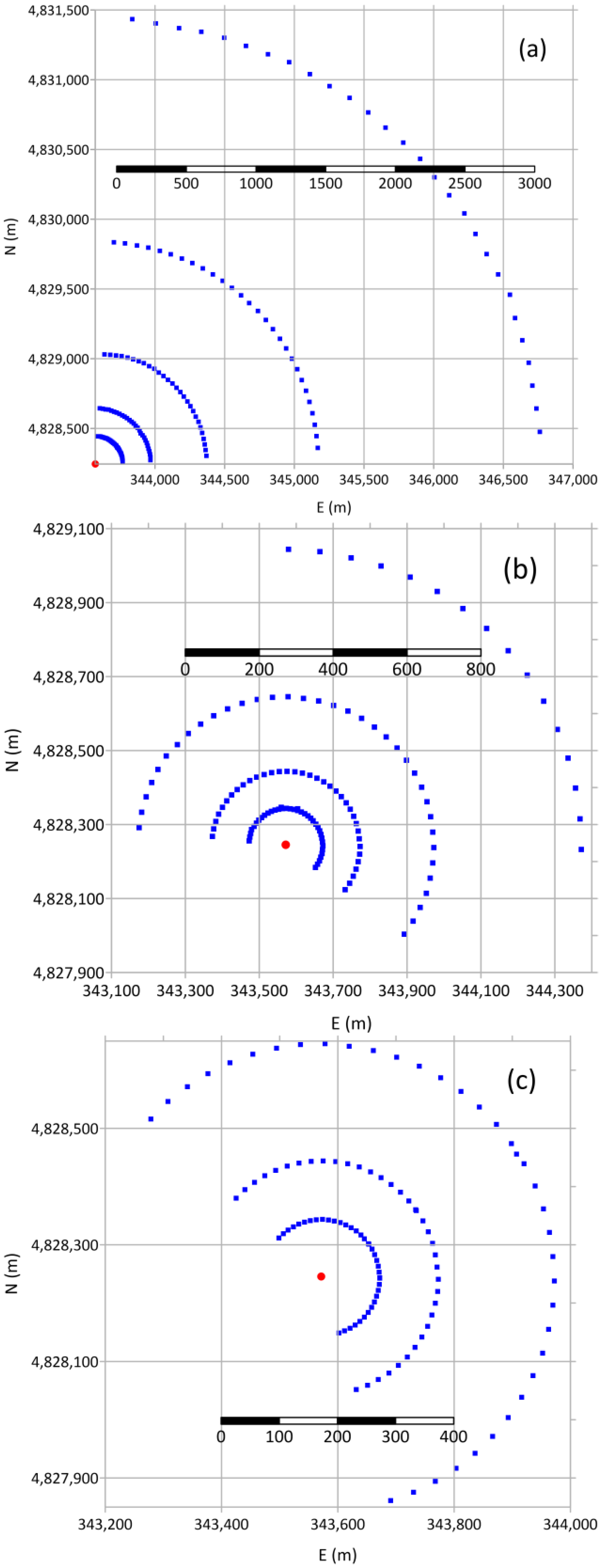
Article

A Comparison of CALPUFF and LAPMOD Against the Project Sagebrush Datasets

by
Roberto Bellasio
1,*,
Roberto Bianconi
1 and
Paolo Zannetti
2
1
Enviroware srl, Via Dante Alighieri 142, 20863 Concorezzo, Italy
2
The EnviroComp Institute, 1188 Eagle Vista Ct., Reno, NV 89511, USA
*
Author to whom correspondence should be addressed.
Atmosphere 2025, 16(6), 671; https://doi.org/10.3390/atmos16060671
Submission received: 2 May 2025 / Revised: 21 May 2025 / Accepted: 26 May 2025 / Published: 1 June 2025
(This article belongs to the Section Atmospheric Techniques, Instruments, and Modeling)

Abstract

This paper presents the validation of CALPUFF and LAPMOD against the short-range and high time resolution tracer study dataset of Project Sagebrush (PSB). The meteorological fields for both models are prepared with the CALMET diagnostic model starting from the exhaustive meteorological data collected during PSB. The PSB releases were undertaken under different meteorological and turbulence conditions. The validation results—judged by means of several statistical parameters—indicate that the models are generally in satisfactory agreement with the observations, sometimes even when time- and space-paired data are considered. However, in four simulations carried out under low wind and very stable conditions, the model performances are poor. This may be due to the inability of CALMET to reproduce the vertical wind direction variations in a shallow layer close to the ground, but also to inappropriate turbulence dispersion algorithms in the dispersion models. This issue will be further investigated in future work.

1. Introduction

Atmospheric dispersion models (ADMs) are important tools to evaluate existing air quality together with monitoring stations. Moreover, they are the only tools capable of predicting future air quality expected after the realization of new industrial plants or modifications of existing ones. The importance of air dispersion models is also recognized both by the previous EU Directive 2008/50/CE [1] on ambient air quality and by the new one 2024/2881 [2]. Additionally, the US-EPA provides a list of preferred models, as well as guidance for their use in predicting the ambient concentrations of air pollutants [3].
Due to their importance, ADMs must be continuously validated against field experiments data to verify their ability to estimate observed concentrations. Some field experiments continue to remain important, but they are becoming dated, since they were conducted in the 1950s and 1960s. The tracer studies include, for example, Kincaid [4], Indianapolis [5] and Prairie Grass [6]. These have been extensively used to validate ADMs (e.g., [7]). A new tracer study named Project Sagebrush (PSB) was performed in 2013 (phase 1, PSB1) [8] and 2016 (phase 2, PSB2) [9] in flat terrain. PSB offers the advantage of using technologies not available during older field experiments, therefore providing a lot of information for understanding atmospheric dispersion and validating both meteorological and dispersion models. During PSB, an inert species (SF6) was released, and concentration measurements were taken with a time resolution of 10 min up to a distance of 3.2 km. These features make PSB very useful for verifying the ability of ADMs to estimate concentrations at relatively short distances and with high time resolution. Therefore, validation against PSB data may also be important to evaluate the ability of a model to simulate odor pollution, that often impacts relatively close to the source.
PSB data have already been used to validate models, mainly meteorological ones. For example, Ngan et al. (2018) [10] used the PSB1 data to evaluate the meteorological field obtained with the WRF meteorological model [11] and the concentrations estimated by the HYSPLIT particle dispersion model [12]. WRF was used with five nested domains, with the grid resolution going from 27 km to 333 m, using inline and offline approaches, as well as different planetary boundary layer schemes and a large-eddy simulation parameterization. HYSPLIT was used to reproduce the concentrations of IOP2, IOP3, IOP4 and IOP5, where IOP indicates Intensive Observation Period, or each release of the field experiment. IOP1 was excluded because the wind flow patterns caused the tracer plume to go in the opposite direction to the sampling array [8].
Similarly, Thomas and Kurzeja (2023) [13] used WRF and HYSPLIT to simulate the PSB1 releases. They implemented a Large Eddy Simulations (LES) model in WRF, and used it with four nested domains with grid resolutions of 3 km, 1 km, 200 m and 67 m. The authors simulated IOP3 and IOP5 and discussed only IOP5. The WRF/LES results were in satisfactory agreement with meteorological observations but the HYSPLIT SF6 concentrations overestimated the observations.
Bhimireddy and Bhaganagar (2018) [14] used WRF with multiple nested domains, starting with a grid size of 24 km, and downscaled it through LES up to a grid size of 150 m. With this approach, they simulated the atmospheric boundary layer (ABL) processes of IOP2-5 during PSB1. WRF was used with three boundary layer schemes, three surface layer schemes and two micro-physics schemes in order to perform a sensitivity analysis. The output of the model was compared to the meteorological observations collected during PSB1.
Finn et al. [15] used the PSB1 data to evaluate the correctness of the parameterization of the horizontal plume spread, whose formulation had been obtained empirically from the results of old tracer experiments. They found that the horizontal plume spread calculated with the modern instrumentation used in PSB1 was larger than that measured in many previous field studies by up to a factor of 2, and the discrepancies tended to increase with downwind distance.
Large and rapid wind direction changes were observed by Finn et al. (2018) [16] in low wind speed conditions in the very stable boundary layer during PSB2. This is in contrast with the common assumption that the plume is very narrow in stable atmospheric conditions due to the small values of the wind direction standard deviation (σθ). The authors observed that these wind direction changes are particularly frequent when the wind speed at 2 m agl is less than 1.5 m/s and are associated with sensible heat and momentum fluxes near zero. Another observation of [16] is that the magnitude of the wind direction changes is larger close to the ground and limited a few meters above it.
Another study investigating the results of PSB2 [17] demonstrated, by means of co-located samplings, that concentration variability at the same place, due to stochastic factors and independent of measurement uncertainty, increases the total observational uncertainty closer to the source from about 20% (daytime) to 40% (very stable conditions). The large increase in concentration variability is linked with the suppression of turbulent mixing, small eddy length scales, and meandering in very stable conditions. These results are really challenging when comparing observations with model predictions.
In this work, the results of PSB1 and PSB2 are used to validate two ADMs. One is the popular Lagrangian puff model CALPUFF [18], and the other one is the Lagrangian particle model LAPMOD [19]. As far as the authors know, this is the first time that both PSB1 and PSB2 have been used to validate ADMs because, as described above, many validations used only few IOPs of PSB1. Validation of ADMs against the PSB2 data, particularly for the four IOPs carried out under very stable conditions, is very challenging.
The first part of this paper describes in detail the Project Sagebrush (PSB), the models and their configurations. Then the results for each IOP of PSB1 and PSB2 are presented and discussed. The validation was performed quantitatively using several statistical parameters that are summarized by a rank introduced to show the behavior of each model at a glance.

2. Materials and Methods

In this paragraph, the methodologies adopted are described in detail to allow other researchers to replicate the results if needed.

2.1. Project Sagebrush

The Air Resources Laboratory’s Field Research Division (ARLFRD), part of the National Oceanic and Atmospheric Administration (NOAA), in collaboration with the Laboratory for Atmospheric Research at Washington State University (WSULAR), conducted a set of tracer releases at the Idaho National Laboratory (INL). The project was divided into two series of releases. PSB1 (Project Sagebrush Phase 1) was carried out in October 2013 during daytime (near-neutral and unstable conditions), while PSB2 (Project Sagebrush Phase 2) was carried out with light wind conditions in July, August (unstable conditions) and October (nighttime stable conditions) in 2016. PSB1 is described in [8], and PSB2 is described in [9].
The field releases were performed at the INL Grid 3 experimental site, which is in an almost flat plain on the western edge of the Snake River Plain in southeast Idaho (USA). The site is about 1500 m above the mean sea level.
Both PSB1 and PSB2 were characterized by the continuous release of SF6 close to ground level. All the releases lasted 2.5 h, while the samplings lasted for two hours, commencing 30 min after the release start in order to establish a quasi-steady-state SF6 concentration field across the sampling array. Many tracer studies were conducted in flat terrain from the 1950s and 1960s (e.g., [4,6]). PSB offers the advantage of using technologies not available during those older studies, therefore providing a lot of information to understand atmospheric dispersion and to validate models.

2.1.1. Source Characterization

In both PSB1 and PSB2, the point source was placed at the center of the INL Grid 3, whose coordinates are 43.59076 N, 112.93782 W, or E = 343,571.59, N = 4,828,245.40 within UTM zone 12T (where the letter T indicates a latitude between 40 and 48 degrees north). The SF6 was contained in two bottles and was released from the outlet end of a garden hose at a height of 1.5 m above ground level. The release diameter was about 5/8″ or 1.59 cm [20]. The garden hose was oriented horizontally to avoid imparting any vertical momentum to the tracer [9]; therefore, the vertical exit speed is considered null.
Five IOPs were realized during PSB1, with the release properties specified in Table 1. The first three IOPs have a release rate about one order of magnitude greater than the last two. The reason is that during IOP1–3, a real-time analyzer was installed within an aircraft, and the release rate was selected in order to provide tracer concentrations sufficiently high to be measured by such an instrument [8]. On the other hand, during IOP4–5, the aircraft was not available.
Four IOPs were conducted with light wind conditions during daylight in July and August 2016. A further four IOPs were conducted in light wind conditions at nighttime during October 2016. Table 2 summarizes the release information for PSB2. The release rates were designed to provide measurable tracer concentrations within the dynamic sampling ranges of the bag and fast response samplers at all sampling distances [9].
Release temperatures were not available for PSB1, while they were available for PSB2. The analysis of the release temperature of IOPs 1–4 of PSB2 that were performed at similar hours to those of PSB1, though in different months, showed that—on average—they are about 5 °C higher than the average air temperature measured at 2 m agl at the GRI meteorological tower during the releases. Therefore, the temperatures reported in Table 1 were obtained by adding 5 °C to the average air temperature measured during the releases of PSB1.
The release temperatures reported in Table 2 were not indicated in the technical reports describing PSB2 [9]. They were calculated by averaging over the 2.5 h of emission the gas temperature reported in the release files with a time resolution of 1 s.

2.1.2. Meteorological Data

Meteorological data were collected with different instruments both in PSB1 and PSB2. This paragraph provides a brief summary of the measures that were collected. The detailed information is available in [8] for PSB1 and [9] for PSB2.
The following instrumentation was common to PSB1 and PSB2:
  • A tower of 62.3 m of height (GRI) over which different instruments were mounted, including sonic anemometers. The GRI was located at an arc distance of 200 m from the INL Grid 3 center (release location) with an angle of 235 degrees. Wind direction and wind speed were measured at different heights above the ground: 2 m, 9.96 m, 15.31 m, 45.1 m and 60.05 m. Air temperature was measured at 1.5 m, 10.7 m, 14.9 m, 45 m and 59.6 m. Solar radiation, barometric pressure and precipitation were also measured at GRI. Three sonic anemometers were placed at heights of 4 m, 30 m and 45 m, and were named G1, G2 and R1, respectively. Four further sonic anemometers were placed at 2 m, 8 m, 16 m and 60 m above the ground.
  • A lower tower (COC) of 30 m was located at an arc distance of 499 m from the INL Grid 3 center with an angle of 60 degrees. Wind speed and direction were measured over this tower at the following heights above the ground: 2 m, 10 m and 30 m. These meteorological variables were available with a time resolution of 5 min in PSB1 and of 10 min in PSB2. For PSB2, the 1 s time resolution files were also available.
  • An energy flux station (FLX) was located at an arc distance of 916 m from the INL Grid 3 center with an angle of 51 degrees. It is a permanent installation designed to measure how the shrub-steppe habitat of the INL interacts with the global energy cycle. Measurements were performed on two separate towers as follows: air temperature, relative humidity, barometric pressure and solar radiation were measured on the tripod of the first tower, while a sonic anemometer (at 3.2 m above the ground) and open path infrared gas analyzer (IRGA) were mounted on the tripod of the second tower.
  • A radar wind profiler (PRO) and a Radio Acoustic Sounding System (RASS) were co-located at an arc distance of 828 m from the INL Grid 3 center with an angle of 56 degrees. The PRO was configured to take measurements of wind speed and direction at 28 levels covering a vertical range from 159 m to 2895 m with a vertical resolution set at 101 m. Wind data were collected for 25 min intervals twice each hour from minute 5 to minute 30 and from minute 35 to minute 60. The RASS was configured to measure air temperature with a vertical resolution of 105 m from 165 m to 1633 m. Temperature data were collected for 5 min intervals twice each hour from minute zero to minute 5 and from minute 30 to minute 35.
  • A minisodar (ASC) was located at an arc distance of 816 m from the INL Grid 3 center with an angle of 57 degrees. It is a remote sensing device that measures the vertical profiles of wind speed and direction in the lowest levels of the atmosphere. The ASC vertical range was set from 30 m to 200 m, with a height resolution of 10 m.
  • Meteorological balloons (radiosonde) were launched at an arc distance of about 400 m from the INL Grid 3 center with an angle of about 55 degrees before and after each IOP. For each IOP, the first balloon was launched about 15 min before the sampling start, and the second balloon was launched about 15 min after the sampling end.
  • Additionally, many meteorological stations managed by ARLFRD are present across the Eastern Snake River Plain covering the test area. These stations measure wind speed and direction, air temperature, relative humidity, precipitation, solar radiation and other variables. Data are averaged over 5 min periods. The stations are classified within two hypothetical rings, based on the distance from the test area. Ring 1 contains the 9 meteorological stations within a radius of 10 miles, while ring 2 contains the 10 meteorological stations located between 10 and 20 miles.
During PSB1 the following meteorological instrumentation was present:
  • A 10 m open lattice aluminum meteorological tower (TOW) was located near the center of the 3200 m arc at about 44.5 degrees arc angle. Cup anemometers and vanes were used to measure wind speed and direction at 2 m and 10 m heights. Due to problems with power supply, TOW did not work during IOP4 and IOP5 of PSB1.
  • A 3D sonic anemometer (R2) was located close to TOW. It measured wind speed, wind direction and turbulence fields at 3.2 m above the ground.
  • A 3D sonic anemometer (R3) was located at an arc distance of 3200 m at 7 degrees arc angle. It measured wind speed, wind direction and turbulence fields at 3.2 m above the ground.
  • A 3D sonic anemometer (R4) was located at an arc distance of 3200 m at 82 degrees arc angle. It measured wind speed, wind direction and turbulence fields at 3.2 m above the ground.
  • A minisodar (ART) was located close to TOW. It suffered the same power supply problems of TOW; therefore, it did not work during IOP4 and IOP5 of PSB1.
During PSB2 the following instrumentation was present for the IOPs from 5 to 8 (October 2016), excluding the sonic anemometer G2, that was present during all the IOPs:
  • A ceilometer was located at an arc distance of about 400 m from the INL Grid 3 center with an angle of about 54 degrees to measure the boundary layer height and clouds base. It did not work in IOP8.
  • Six 3D sonic anemometers were located at different positions to measure wind speed, wind direction and turbulence fields. The height above the ground was about 3 m for all the instruments. G2 (present during all the IOPs) was located at an arc distance of 1000 m at 150 degrees arc angle. EC1, EC2 and ST2 were located at an arc distance of 400 m at 25, 85 and 150 degrees arc angle, respectively. ST1 and ST3 were located at an arc distance of 800 m at 25 and 277 degrees arc angle, respectively.
It is evident from this brief description that Project Sagebrush is important not only to validate air dispersion models, but also to validate meteorological models, as done, for example, by [10,13,14].

2.1.3. Samplings

SF6 concentrations were measured with programmable bag samplers that acquired time-sequenced air samples in 12 individual Tedlar® bags for each measurement point. The sampling time for each bag was 10 min in order to cover each of the 2 h long IOPs. The samples were then analyzed at the Tracer Analysis Facility (TAF) in Idaho Falls, ID, by means of gas chromatographs (GC). A full description of the sampling procedure is available in [8,9].
During PSB1, a total of 112 primary bag samplers were deployed on four sampling arcs during each IOP. For IOPs 1–3, these samplers were deployed on the 400 m, 800 m, 1600 m and 3200 m arcs. For IOPs 4 and 5, the samplers were deployed on the 200 m, 400 m, 800 m and 1600 m arcs. These samplers were at 1 m agl. Additionally, other samplers were deployed at different heights above the ground at three positions: at 201 m from the source with an angle of 53 degrees (1 m, 5 m, 10 m and 15 m agl); at 408 m from the source with an angle of 59 degrees (1 m, 5 m, 10 m, 15 m and 20 m agl); at 499 m from the source with an angle of 60 degrees (1 m, 5 m, 10 m, 15 m, 20 m, 25 m and 30 m agl). The angles are clockwise from north. Twenty-two other samplers were deployed for quality control purposes. They included 16 field duplicates, 3 field control, and 3 field blank samplers.
During PSB2, 150 samplers were deployed for each IOP; they were mounted at 1 m agl. For the daytime IOPs (IOPs 1–4), 36 samplers were placed along each of the 100 m, 200 m and 400 m arcs. They were placed at 6-degree intervals from 276 degrees azimuth to 126 degrees azimuth. Additionally, 16 samplers were deployed on the 800 m arc at 6-degree intervals from 0 degrees azimuth to 90 degrees azimuth. For the nighttime IOPs (IOPs 5–8), 36 samplers were placed along each of the 100 m, 200 m and 400 m arcs at 6-degree intervals from 312 degrees azimuth to 162 degrees azimuth. For the daytime IOPs, vertical sampling was conducted at 1 m, 5 m, 10 m, 15 m, 20 m and 25 m agl on the 100 m arc, at an angle of 24 degrees for IOPs 1–2, and 352 degrees for IOPs 3–4. For the nighttime IOPs, vertical sampling was conducted at the same heights on the 400 m arc at an angle of 57 degrees. Additionally, bag samplers were deployed on four fixed 10 m towers on the 100 and 200 m arcs at 1, 3, 6 and 9 m heights. As for PSB1, other samplers were deployed for quality control purposes.

2.2. Simulation Models

2.2.1. CALMET

CALMET [21] is a diagnostic meteorological model which reconstructs the 3D wind and temperature fields and micrometeorological variables (e.g., mixing height, Monin–Obukhov length, friction and convection velocity) starting from meteorological measurements—at the surface and at upper layers—and/or output of a prognostic model, and geophysical data (orography and land use).
The micro-meteorological parameters are needed by the dispersion models to calculate their turbulent dispersion coefficients according to the different parameterizations implemented. The unformatted output of CALMET is directly read both by CALPUFF and LAPMOD, without the need for any post-processing.
The diagnostic module uses a two-step approach for the computation of the wind field. In the first step, an initial guess wind field is adjusted for kinematic effects of terrain, slope flows and terrain blocking effects. The second step consists in an objective analysis procedure to introduce observational data into the wind field of the first step to produce a final wind field.
CALMET version 6.5.0, level 150223 was used in this study to produce the output variables with a time step of 300 s (5 min).

2.2.2. CALPUFF

CALPUFF [18] is a Lagrangian puff dispersion model belonging to the list of alternative models of the US-EPA [22]. Alternative models are those that can be used in regulatory applications with case-by-case justification to the Reviewing Authority in situations where the preferred models are not applicable or available. The puffs are advected by the average wind along their vertical extension, while the atmospheric turbulence has the effect of increasing their size [18]. When puffs become very high, wind shear cannot be correctly described. For this reason, CALPUFF includes a “puff-splitting” algorithm that allows splitting of puffs under specific conditions.
CALPUFF is capable of simulating many types of sources, including point, area, buoyant line and volume. Starting from version 7, CALPUFF is also capable of simulating road sources.
The model calculates the concentration at a specific receptor by summing the contribution of each puff at such positions with an analytical expression [23].
CALPUFF version 7.2.1 level 150618 was used in this study.

2.2.3. LAPMOD

LAPMOD [19] is an open source Lagrangian particle model that simulates many types of sources. Computational particles are transported by the combination of the wind at their height and a random component, which is calculated according to the turbulence level [24].
Two numerical plume rise schemes are implemented in LAPMOD for point sources: Janicke and Janicke [25] and Webster and Thomson [26]. LAPMOD describes the orientation of the stack tip by means of two angles: the azimuthal angle (stack orientation on the horizontal plane) and the polar angle (tilting of the stack with respect to the vertical). Rain-capped stacks can also be simulated.
The concentration fields in LAPMOD are calculated with kernel methods (e.g., [27]), that allow using relatively fewer particles with respect to Lagrangian particle models that adopt a counting method to calculate concentrations [28].
Validations of LAPMOD against the experimental datasets of Kincaid (rural conditions), and Indianapolis (urban conditions) can be found in [29,30]. The results of the two validations describe LAPMOD as a reliable model according to the performance evaluation criteria proposed by [31] that are based on FA2, NMSE and fractional bias [32]. An intercomparison between LAPMOD and other dispersion models for odor applications was presented in [33]. Another intercomparison between LAPMOD and CALPUFF, specifically for rain-capped and horizontal stacks, is discussed in [34]. Finally, [35] described the introduction in LAPMOD of a modified turbulence scheme to better represent the dispersion of radionuclides at a Chinese nuclear power plant when buildings are present. Their results show that agreement between wind tunnel observations and model predictions increases when the new scheme is activated. This may be an important result when considering odor pollution, because buildings are often present and the impacts occur over relatively short ranges.
LAPMOD version 2025-03-25 was used in this study.

2.2.4. Configuration of the Two Dispersion Models

The emissions were determined by means of a point source placed 1.5 m agl with a diameter of 1.59 cm. Since the release direction was horizontal, the vertical mechanical momentum was suppressed by forcing the exit velocity to 0.001 m/s, as suggested by the US-EPA [36]. The release temperature and release rate for each IOP are reported in Table 1 and Table 2.
The values used for the most important input variables are summarized in Table 3 and Table 4, respectively, for CALPUFF and LAPMOD.
The stack tip downwash (STD) was not activated because the release is horizontal and, in any case, the release diameter is very small (the effect of STD is to decrease the stack height by a maximum of 3 diameters). Dry and wet deposition were not activated.
The positions of the discrete receptors (sampling sites) used to validate the models in this study are represented in Figure 1 by means of blue squares, while the red circle represents the source location. All the receptors are placed at 1 m agl. It is noted that the three panels of Figure 1 have different scales. During PSB1 (Figure 1a), the receptors placed from 400 m to 3200 m from the source were used for IOP1-3, while the receptors placed from 200 m to 1600 m from the source were used for IOP4-5. Concerning PSB2, the receptors used in convective conditions during the summer (IOP1-4) are shown in Figure 1b, while those used in stable conditions during the nights or in the late afternoon of October are shown in Figure 1c.

2.3. Meteorological Fields of Each IOP

As described above, a lot of meteorological instrumentation was present within and around the area of study. Therefore, considering also that the area is practically flat, the meteorological fields during the IOPs were determined using only the CALMET diagnostic meteorological model [21]. An alternative procedure would be, for example, to use—in addition to CALMET or alone—a prognostic meteorological model like WRF [11], as performed for example in [10,13]. However, in this work it is assumed that, over such a small area, the meteorological fields can be reliably reproduced using the extensive meteorological measurements that were carried out in PSB.

2.3.1. CALMET Domain

The domain of the CALMET meteorological model is shown in Figure 2. The UTM coordinates of its lower left corner are E = 336,000, N = 4,821,000 within zone 12T. In each direction, 70 grids were used, with a resolution of 200 m; therefore, the size of the square domain is 14 km. A smaller grid size (i.e., better spatial resolution) was not deemed necessary because the area of interest is mostly flat.
The terrain level over the simulation domain was determined with the SRTM data (Shuttle Radar Topography Mission) [37] with a spatial resolution of about 30 m on the line of the equator. The average terrain level over the 200 m grids ranges from 1471 m (northeastern part of the domain) to 1554 m (northwestern part of the domain). The average terrain elevation over the CALMET domain is 1502 m. The Copernicus Global Land Cover Dataset 2019 [38] with a resolution of 100 m was used for describing the land use. Almost all the grid cells (99.3%) are classified with the land use “rangeland”, which is associated with a roughness length z0 of 5 cm. This value is in good agreement with those found in [8,9,15] using wind profiles: a median z0 of 3 cm for SW winds (typically, common during the day), and a median z0 of 3.8 cm for NE winds (typically, common during the night).
Along the vertical direction, 12 levels were used, with the top of domain at 4000 m agl.

2.3.2. Surface Meteorological Data

The available surface meteorological measurements collected during PSB were redundant when running CALMET; therefore, some of them were not used in input to the model. For example, the Mesonet station GRI that measures wind at 15 m agl was located exactly where the 62.3 m high tower was located; therefore, its measurements are redundant. After verifying that the Mesonet GRI wind and the wind at 15 m at the tower were comparable, it was decided to keep the observations at the tower.
Cloud cover and sky altitude were obtained from the two ASOS stations closest to the test area: Pocatello Regional Airport (PIH), located approximately 80 km SSE from the test area, and Friedman Memorial Airport (SUN), located approximately 110 km west from the test area. The ASOS data were downloaded from the Iowa State University internet site [39]. These data report sky altitude in feet, while cloud cover is reported with a 3-letter category (e.g., CLR, FEW, SCT). Following the indications presented in Table 3 of [40], an equivalence was established between the category and the cloud cover in tenths needed by CALMET, as reported in Table 5. Data were available with a time resolution of 1 h in 2013 (PSB1) and of 5 min in 2016 (PSB2) in station PIH, while they were available with a time resolution of 20 min in both 2013 and 2016 in station SUN. Cloud cover and ceiling height for CALMET were determined starting from the data of the closest station (PIH) with the intention to consider the second station (SUN) only as a backup when one of the two variables was not available in PIH. In the event, there was no need to use the SUN data because the PIH data were complete. The cloud cover and ceiling height in PSB1 varied every 60 min or 20 min, while in PSB2, they varied every 5 min or 20 min. These two variables were considered uniform over the whole domain.
The observations of the following “surface stations” were used to feed CALMET in both PSB1 and PSB2:
  • GRI Tower (62 m) at a height of 2 m agl. The ceiling height and cloud cover from the PIH ASOS station were assigned to this station. The code used in CALMET to identify this station is 10002.
  • Five Mesonet stations within the CALMET domain (excluding GRI): 690, LOS, NRF, PBF and TRA. The codes used in CALMET to identify these stations are 12001 (690), 12002 (LOS), 12003 (NRF), 12004 (PBF) and 12005 (TRA).
  • COC Tower (30 m) at a height of 2 m agl (only wind speed and direction). The code used in CALMET to identify this station is 11002.
Additionally, three 3D sonic anemometers R2, R3 and R4 (station codes: 13002, 13003 and 13004) were used in PSB1, while TOW was not used due to the power supply problems in IOP4 and IOP5. During PSB2, the G2 sonic anemometer was used (station code 14003), except in IOP4, in which it was not available.
The UTM12T coordinates and the anemometer height of the meteorological stations used in CALMET are summarized in Table 6. The position of the surface meteorological stations with respect to the source is shown in Figure 2.
In CALMET, the wind measured by surface stations, within the routine DIAGNO, is always extrapolated from the anemometer height to first model the vertical level using a neutral log profile over land. This means that, since the first (lower) vertical cell in CALMET must be from the ground (0 m agl) to 20 m agl, and the horizontal wind components are calculated in the middle of this cell, the lower height at which wind is available is 10 m agl. Then, when many observations were available at different heights at the same position—as for the GRI and COC towers—only the lower measurements were used, to avoid wind extrapolation at 10 m agl from the measurements carried out, for example, at 2 m, 15 m, 20 m, etc. The choice to consider the observations of lower height is because they are the most representative for the release (source height is 1.5 m agl), and the lowest observation height at the towers is 2 m agl.
The meteorological variables measured by the COC tower are available with a time resolution of 5 min in PSB1 and 10 min in PSB2. For PSB2, the 1 s time resolution files were also available. In order to use the same time resolution (5 min) in both phases, a Python program (version 3.9.1) was developed to obtain the 5 min averages from the 1 s ones. To check the correctness of the Python program, it was used to calculate the 10 min averages, that were then compared with those already available in the dataset.
The SURFCSV meteorological processor of CALMET was used to prepare the surface meteorological file of each single station; then, the different files of a specific IOP were merged to obtain a single SURF.DAT file.

2.3.3. Upper Air Meteorological Data

The CALMET simulation must start before 5 LST to correctly initialize the mixing height; also, the radio soundings must be available before and after the initial and final simulation times. During PSB local radio soundings were performed 15 min before and after the tracer release; then, excluding IOP5-7 of PSB2, the initial sounding was always after 5 LST (see Table 1 and Table 2). Therefore, additional radio soundings were needed to carry out the CALMET simulations. These vertical data were collected from the Boise airport (USAF: 72681) located about 264 km west of the release site, at a height of 874 m asl. The Boise vertical profiles were downloaded from the internet site of the University of Wyoming, Department of Atmospheric Science [41]. On 4 and 5 August 2016 (IOP3 and IOP4 of PSB2) some vertical profiles were not available from the University of Wyoming. Therefore, for those two days, the vertical profiles were downloaded from the IGRA (Integrated Global Radiosonde Archive) [42].
Also, the initial local vertical profile (the one starting approximately 15 min before the sampling) for IOP6 of PSB2 (20 October 2016) was not available, probably due to technical problems. Therefore, in order to perform the CALMET simulation, the Boise profile was used.
The final UP.DAT files used in input for each CALMET simulation were obtained by merging the local and the Boise vertical profiles. Each UP.DAT file contains the values of pressure, height above sea level (asl), temperature, wind direction and wind speed for different vertical levels. The maximum height considered was 10,000 m asl.
The launch position of the local radio soundings was very close to the COC surface station shown in Figure 2.

2.4. Statistical Parameters

The following statistical indexes were used to quantitatively evaluate the models’ performances (e.g., [32,43]): percent of predictions within a factor of 2 (FA2) and 5 (FA5) from the observations, factor of exceedance (FOEX), correlation coefficient (R), fractional bias (FB), normalized mean square error (NMSE) and figure of merit in space (FMS).
The FAα, where typically α = 2 and/or α = 5, is determined as the percentage of values that satisfy Equation (1), with Pi and Mi that are the i-th prediction and measurement, respectively.
1 α P i M i α
The FOEX is determined as the number of overpredictions N(Pi > Mi), divided by the total number N of data, minus 0.5, and expressed as a percentage (Equation (2)). Therefore, it ranges from −50% (the model always underpredicts) to +50% (the model always overpredicts).
F O E X = 100 × N P i > M i N 0.5
The correlation coefficient R is defined by Equation (3), where the overbars represent the average value. R ranges between −1 and +1. A value R = +1 (complete positive correlation) corresponds to all the pairs (Mi, Pi) laying on a straight line with positive slope in the scatter diagram. The complete negative correlation (R = −1) corresponds to all the pairs on a straight line with negative slope. A value of R near to zero indicates the absence of correlation between the observations and predictions.
R = i = 1 N M i M ¯ P i P ¯ i = 1 N M i M ¯ 2 i = 1 N P i P ¯ 2
The fractional bias (FB) is defined as shown by Equation (4). FB ranges from −2 to +2, where positive values indicate overprediction and negative values indicate underprediction.
F B = 2 P ¯ M ¯ P ¯ + M ¯
The normalized mean square error (NMSE) is defined by Equation (5). It is always a positive number giving information about the deviation between predictions and measurements.
N M S E = 1 N i = 1 N P i M i 2 P ¯ M ¯
The figure of merit in space (FMS) is calculated as the intersection over the union of predicted p and measured m concentrations in terms of the number N of samples with concentrations greater than a given threshold [43]. The threshold used in this analysis has been chosen arbitrarily as a small value (5 ppt).
F M S = 100 × N p N m N p N m
In order to evaluate the model performances at a glance, without considering in detail all the statistical indexes, a rank was defined by combining those indexes, similarly to the procedure described in [43]. A rank ranging from 0 (worst model performance) to 5 (best model performance) was defined in this study as:
Rank = R + (1 − |FB/2|) + (1 − 2 |FOEX|/100) + FA5/100 + FMS/100
The conversion from the concentration values calculated by the two models (in µg/m3 or ng/m3) to concentrations (mixing ratio) expressed in pptV was carried out as in [8], considering the mean atmospheric temperature (K) and pressure (Pa) at GRI during each of the two-hour release periods.
A background of 9 ppt was subtracted from all SF6 observations of PSB1 and negative values set to zero, as performed, for example, in [13]. The value of 9 ppt was chosen because it is the ceiling of the average value reported in the paragraph titled “Atmospheric background checks of SF6 at the tracer analysis facility” in [8]. Concerning PSB2, the same paragraph in [9] reports a background value a bit higher; therefore, with similar reasoning, the background value used for PSB2 was 10 ppt.

3. Results and Discussion

The results are presented in the following subparagraphs for each IOP, both by pairing in time and space the observed and predicted concentrations, both by time-averaging the observed and predicted concentrations at each sampling point over the 2-hour-long sampling interval. Of course, the comparison of time-paired data is more demanding; therefore, lower agreement between observations and predictions is expected with respect to the time-averaged data.
For each IOP, the 5 min CALMET data were extracted at the release location (E = 343,571.59, N = 4,828,245.40, UTM zone 12T) for the first vertical level (10 m agl) and for the 2 h length of the sampling interval (i.e., without considering the first 30 min of the release). The wind roses obtained from those data are then represented to better understand the fate of the SF6 plume. It is anticipated that, for PSB1, the wind roses obtained in this work would be quite similar to those reported in [14]. No wind roses were found in the scientific literature for PSB2.
The statistical analysis was carried out by considering only the observations associated with quality flags lower than 3 (values flagged with 3 or more are of bad quality) [8,9].

3.1. PSB1–IOP1

As reported by [8], during IOP1 conducted on 2 October 2013 from 14:30 to 16:30 MST, winds were very light and variable with mostly sunny conditions but filtered through patchy cirrostratus. Overall conditions were highly non-stationary and the adverse wind directions made for generally poor tracer sampling. The wind rose obtained from CALMET at the release location (Figure 3) is consistent with such a description. Calms (i.e., winds below 0.5 m/s) are predicted for 25% of the time. The average wind speed determined by CALMET during IOP1 is 0.9 m/s, with a maximum value of 2.0 m/s. The mode of the wind speed distribution is between 1 m/s and 2 m/s, with exactly 50% of the events. The wind blows prevalently from E-SE; therefore, the cloud is going to miss the sampling sites represented in Figure 1a most of the time. Indeed, as shown, for example, in Figure 4, the computational particles of LAPMOD at the end of the IOP (16:30 MST) close to the source are directed toward the west, while higher particles, far from the source, go toward the northeast, lightly impacting on the sampling points close to north (i.e., those with smaller angles). However, since these particles are relatively high over the ground, the calculated concentration values are small.
The Pasquill–Gifford (PG) stability classes calculated by CALMET for PSB1-IOP1 are always very unstable (class B, excluding class C during the first five minutes of the release).
Since the SF6 cloud is missing the sampling points, the statistical analysis is not reported for PSB1-IOP1.

3.2. PSB1–IOP2

During IOP2 of PSB1, conducted on 5 October 2013 from 13:00 to 15:00 MST, the weather was mostly sunny, and the winds were generally relatively light (under 3 m/s) during the first half of the release, increasing somewhat over the second half. Wind directions varied but were consistently southwesterly with few exceptions. This description, reported by [8], agrees with the wind rose obtained with CALMET at the release location (Figure 5). The average wind speed determined by CALMET during IOP2 is 3.1 m/s, with a maximum value of 5.0 m/s. The mode of the wind speed distribution is between 2 m/s and 3 m/s, with 45.8% of the events. The PG stability classes calculated by CALMET for PSB1-IOP2 are very unstable for the first 75 min of the release (class B), then evolve to moderately unstable (class C) for the remaining time, excluding the last five minutes, that are class D.
The statistical parameters calculated for CALPUFF and LAPMOD are summarized in Table 7. Considering the time- and space-paired data (N = 1489), the two models predict almost the same maximum concentration value, which is more or less double the maximum observation. The values of FA2 and FA5 are comparable for the two models. The FOEX indicates that LAPMOD slightly underpredicts, while CALPUFF overpredicts. The ranks indicate better agreement of LAPMOD with the observations with respect to CALPUFF.
Concerning the time-averaged concentrations at each sampling point of the four arcs, the statistical parameters in Table 7 show a good agreement of LAPMOD with the observations. The ratio between the LAPMOD and the CALPUFF ranks is close to or greater than 2. Also, for the arcs at 400 m and 800 m, the LAPMOD rank is at least 4, with the best theoretical value equal to 5. Even at the arc of 3200 m, the LAPMOD rank is close to 4. The time-averaged concentrations at each sampling point of the arcs are represented in Figure 6.

3.3. PSB1–IOP3

As described by [8], IOP3 of PSB1 was conducted on 7 October 2013 from 13:00 to 15:00 MST. The weather was mostly sunny, and winds were consistently moderate to strong, in excess of 7 m/s throughout the release under generally clear skies, and wind directions were consistently southwesterly and showed minimal variation. All estimates of stability indicate near-neutral conditions. Flows exhibited a high degree of spatial and temporal homogeneity and stationarity. This description is in complete agreement with the wind rose obtained with CALMET at the release location (Figure 7), which shows only two directions: SW, the prevailing one, and SSW. The average wind speed determined by CALMET during IOP3 is 8.8 m/s, with a maximum value of 10.3 m/s. All the wind speeds are above 6 m/s; for this reason, the PG stability classes calculated by CALMET for PSB1-IOP3 are always neutral (class D).
As shown by the statistical parameters summarized in Table 8, the two models predict quite well the observed concentrations, with CALPUFF showing results that are slightly better than LAPMOD. Considering the time- and space-paired data (N = 1488), the statistical parameters calculated for the two models are very similar; indeed, the final ranks calculated are also similar: 3.5/5 for LAPMOD and 3.8/5 for CALPUFF.
The time-averaged concentrations at each sampling location over the arcs are shown in Figure 8. The concentration distribution over the sampling locations is more or less Gaussian, with the maximum values at the central angles. At the closest arcs, LAPMOD predicts quite well the maximum values, while it underpredicts the lower values at the borders of the arcs. However, notwithstanding this qualitative positive evaluation of LAPMOD, according to the ranks, CALPUFF behaves better in three of the four arcs, with values of at least 4 (where the maximum is 5).

3.4. PSB1–IOP4

As described by [8], IOP4 of PSB1 was performed on 11 October 2013 from 14:00 to 16:00 MST. The weather was mostly sunny, and the meteorological conditions were similar to those observed during IOP3 with some differences. The wind speeds and turbulence were generally lower and winds were generally favorable (i.e., blowing toward the sampling sites) southwesterly. Indeed, the wind rose obtained with CALMET at the release location (Figure 9) shows wind speeds a bit lower than those reconstructed for IOP3 (Figure 7), and the prevailing direction is SW. The average wind speed determined by CALMET during IOP4 is 5.1 m/s, with a maximum value of 6.4 m/s. The mode of the wind speed distribution is between 5 m/s and 6 m/s, with 41.7% of the events. The PG stability classes calculated by CALMET for PSB1-IOP4 are C and D during the first hour of the release, then almost always D during the second hour.
The statistical parameters calculated for IOP4 are summarized in Table 9 and show that the two models predict quite well the observed concentrations, with LAPMOD showing results that are slightly better than CALPUFF. The global analysis with time- and space-paired data (N = 1464) shows that the maximum 10 min average concentration is better predicted by LAPMOD (exceeding the observed value a little) with respect to CALPUFF (underestimating the observed value). On the other hand, the remaining statistical indexes are slightly better for CALPUFF than for LAPMOD, resulting in a final rank slightly better for CALPUFF (3.7/5) than for LAPMOD (3.5/5). Then, as for PSB1-IOP3, the final ranks of the global analysis are similar.
The time-averaged concentrations at each sampling location over the arcs are shown in Figure 10. As for PSB1-IOP3, the concentration distribution over the sampling locations is more or less Gaussian, with the maximum values at the central angles. At the closest arc, both models predict very well the time-averaged observations with a rank of 4.6/5. At the remaining three arcs, the agreement between CALPUFF and the observations decreases, while the one between LAPMOD and the observations remains high, with ranks greater than 4 at the 400 m and 800 m arcs, and a rank of 3.7/5 at the farthest arc (1600 m).

3.5. PSB1–IOP5

IOP5 of PSB1 was performed on 18 October 2013 from 13:00 to 15:00 MST. As described by [8], the weather conditions were similar to those of IOP3 and IOP4: the sky was mostly sunny, and wind came from the SW quadrant. As reported, wind speeds increased from about 3–4 m/s at the start of the tracer sampling period (13:00) to 3–6 m/s at the end (15:00).
The wind rose obtained with CALMET at the release location (Figure 11) is in agreement with the description of the weather conditions, also showing more directional variability with respect to IOP3 and IOP4. The prevailing direction is again SW. The average wind speed determined by CALMET during IOP5 is 4.6 m/s, with a maximum value of 5.2 m/s. The mode of the wind speed distribution is between 4 m/s and 5 m/s, with 66.7% of the events. The PG stability classes calculated by CALMET for PSB1-IOP5 are B and C during the first 40 min of the release, then C and D for the rest of the release.
The statistical parameters calculated for IOP5 are summarized in Table 10. As for IOP4, they show that the two models predict quite well the observed concentrations, with LAPMOD showing results that are slightly better than CALPUFF, particularly for the farthest arc (1600 m). The global analysis with time- and space-paired data (N = 1502) shows that the statistical indexes calculated from the results of the two models are very similar; indeed, the final ranks are 3.8/5 and 3.6/5, respectively, for LAPMOD and CALPUFF.
The time-averaged concentrations at each sampling location over the arcs are shown in Figure 12. Again, the concentration distribution over the sampling locations is more or less Gaussian, with the maximum values at the central angles. The charts show that, excluding the closest arc (200 m), CALPUFF has a general tendence to overestimate the observations. At the closest arc, both models predict very well the time-averaged observations, with a rank of 4.2/5 for LAPMOD and 4.7/5 for CALPUFF. As observed for IOP4, at the remaining three arcs, the agreement between CALPUFF and the observations decreases, while the one between LAPMOD and the observations remains high: 4.2/5 at the 400 m arcs, 3.9/5 at the 800 m arcs, and 3.6/5 at the farthest arc (1600 m). At the farthest arc the CALPUFF rank drops to 1.9/5.

3.6. PSB2–IOP1

IOP1 of PSB2 was performed on 26 July 2016 from 12:00 to 14:00 MST. As described by [9], the weather conditions were hot and dry with light and variable winds throughout the IOP. The skies were clear and sunny during the first hour of the measurement period with some cloudiness during the second hour. Overall conditions were unstable and highly non-stationary in both time and space.
The wind rose obtained with CALMET at the release location (Figure 13) shows great variability of the wind, both for direction and intensity. Considering the positions of the sampling sites during this IOP (Figure 1b), a certain mass of SF6 was not sampled, specifically, the one emitted while wind was blowing from NE. The average wind speed determined by CALMET during IOP1 is 2.3 m/s, with a maximum value of 4.1 m/s. The mode of the wind speed distribution is between 2 m/s and 3 m/s, with 45.8% of the events. The PG stability classes calculated by CALMET for PSB2-IOP1 are always very unstable (A or B).
The statistical parameters calculated for PSB2-IOP1 are summarized in Table 11. The global analysis with time- and space-paired data (N = 1507) shows that the values of FA2 and FA5 are relatively small for both the two models. The final ranks are 3.1/5 for LAPMOD and 2.6/5 for CALPUFF; therefore, it seems that LAPMOD is more in agreement with the observations with respect to CALPUFF.
The time-averaged concentrations at each sampling location over the arcs are shown in Figure 14. Excluding the closest arc (100 m), CALPUFF generally overestimates the observations. The behavior of the models at the first arc is similar, with a final rank of 3.9/5 for LAPMOD and 4.1/5 for CALPUFF. At the other three arcs, the agreement between LAPMOD and the observations remains good, with ranks ranging from 3.5/5 (800 m arc) to 4.2/5 (200 m arc), while the one between CALPUFF and the observations decreases, with ranks in the range 2.1/5 to 2.8/5.

3.7. PSB2–IOP2

IOP2 of PSB2 was performed on 27 July 2016 from 11:30 to 13:30 MST. According to the technical report describing PSB2 [9], the weather conditions were hot and dry with wind speeds near 3 m/s over most of IOP2. The skies were clear and sunny. Overall conditions were unstable and highly non-stationary in both time and space. Estimates of stability based on traditional Pasquill–Gifford (PG) schemes were mainly class B with some class A and C. The tracer plume was mostly confined to the bag sampling array although wind directions sometimes advected part of the plume away from the sampler array.
The wind rose obtained with CALMET at the release location (Figure 15) shows that the wind blows prevalently from SSW and SW. There are also few winds from ENE that move SF6 outside the sampling locations shown in Figure 1b. The average wind speed determined by CALMET during IOP2 is 3.5 m/s, with a maximum value of 4.8 m/s. The mode of the wind speed distribution is between 3 m/s and 4 m/s, with 58.3% of the events. The PG stability classes calculated by CALMET for PSB2-IOP2 are always very unstable (A or B).
The statistical parameters calculated for PSB2-IOP2 are summarized in Table 12. The global analysis with time- and space-paired data (N = 1521) shows that some statistical parameters are better for one model and some others for the other one. For example, the FA2 for LAPMOD exceeds the one for CALPUFF, while the opposite is true for FA5. Again, correlation is better for CALPUFF, while FB is better for LAPMOD. Accordingly, the final ranks are similar, with 3.1/5 for CALPUFF and 3.0/5 for LAPMOD.
The time-averaged concentrations at each sampling location over the arcs are shown in Figure 16. At the closest arc (100 m), CALPUFF performs well, with an FA2 equal to 82.9% and FA5 equal to 91.4%; the correlation is also good, and the FMS is 100%. As a result, the CALPUFF rank at 100 m is 4.1/5, while the LAPMOD rank is 3.9/5. Figure 16 shows that LAPMOD overpredicts the observations at the central angles of the closest arc. At the remaining three arcs, the agreement between LAPMOD and the observations is higher than the agreement between CALPUFF and the observations, with the LAPMOD ranks ranging from 2.5/5 (800 m arc) to 3.5/5 (200 m arc), and the CALPUFF ranks ranging from 1.1/5 (800 m arc) to 3.0/5 (200 m arc). In particular, as shown by Figure 16 and by the FOEX values in Table 12, CALPUFF always overpredicts the observations at the three farthest arcs.
At the 200 m arc, the maximum values predicted by the models are at angles within the range 18–30 degrees, while the maximum observed values are close to 54–60 degrees. A similar shift is also observed at the 400 m arc.

3.8. PSB2–IOP3

IOP3 of PSB2 was performed on 4 August 2016 from 13:00 to 15:00 MST. According to the technical report describing PSB2 [9], the weather conditions were warm and dry, with clear skies and light and very variable winds throughout the IOP. Overall conditions were unstable and highly non-stationary in both time and space. Estimates of stability based on traditional PG schemes were all class A during the first hour and a mix of class A and B in the second hour. There was considerable variation in wind direction, both in time and space.
The wind rose obtained with CALMET at the release location (Figure 17) shows the high variability in wind direction. Some directions do not transport the plume over the sampling locations shown in Figure 1b, for example, those from NE and NNE. Calms (i.e., winds below 0.5 m/s) are predicted for 4.2% of the time. The average wind speed determined by CALMET during IOP3 is 2.1 m/s, with a maximum value of 5.0 m/s. The mode of the wind speed distribution is between 1 m/s and 2 m/s, with 54.2% of the events. The PG stability classes calculated by CALMET for PSB2-IOP3 are always very unstable (A or B, with also C for a short time). More specifically, class A was determined for the first 50 min of the simulation, while the rest of the time was always B, excluding 10 min with C.
The statistical parameters calculated for PSB2-IOP3 are summarized in Table 13. The global analysis with time-paired data (N = 1538) shows that the statistical parameters calculated for LAPMOD—even though not very good—are almost always better than those calculated for CALPUFF. The FOEX index equal to 43.4% implies that CALPUFF overestimates almost always. Indeed, the LAPMOD rank is 2.3/5, while the CALPUFF one is 1.6/5.
The situation improves a bit when the time-averaged concentrations over the arcs are considered (Figure 18). Even the time-averaged CALPUFF predictions always overpredict the time-averaged observations, excluding a couple of points at the first arc (100 m). The FOEX index calculated for CALPUFF is 44.6% at the first arc and 50% at the remaining 3 arcs. Also, for the two farthest arcs (400 m and 800 m), both FA2 and FA5 for CALPUFF are zero. The ranks at the first arc are 3.5 for LAPMOD and 2.6 for CALPUFF. The worst agreement between models and observations is at the farthest arc (800 m) with a rank of 2.3 for LAPMOD and 1.1 for CALPUFF:

3.9. PSB2–IOP4

IOP4 of PSB2 was performed on 5 August 2016 from 12:30 to 14:30 MST. According to the technical report describing PSB2 [9], the weather conditions were warm and dry with mostly sunny skies at the start of the test, with cirrus clouds gradually building over the course of the test period. The winds were light, generally less than 3 m/s, and rather consistently northeasterly. Overall conditions were unstable but were the closest to achieving stationarity of any of the daytime IOPs. Estimates of stability based on traditional PG schemes were mostly class A in the first hour and class C in the second hour. Wind directions were such that the tracer plume missed the bag sampling array in whole or part throughout the measurement period.
The wind rose obtained with CALMET at the release location (Figure 19) shows the winds blow from the whole arc from N to NE, with few exceptions. As observed in the technical report describing the experiment [9], the wind directions were such that the tracer plume missed the sampling locations (Figure 1b) most of the time. The average wind speed determined by CALMET during IOP4 is 2.3 m/s, with a maximum value of 3.1 m/s. The mode of the wind speed distribution is between 2 m/s and 3 m/s, with 70.8% of the events. The PG stability classes calculated by CALMET for PSB2-IOP4 are always very unstable (A or B). More specifically, class A was determined for the first 70 min of the simulation, while the rest of the time it was in class B. Class C mentioned by [9] in the description of IOP4 was not predicted.
The statistical parameters calculated for PSB2-IOP4 are summarized in Table 14. The global analysis with time-paired data (N = 1533) shows that the statistical parameters are not very good for both models. For example, the FA2 value is about 30% for LAPMOD and about 20% for CALPUFF. The ranks are 2.7/5 and 2.1/5, respectively, for LAPMOD and CALPUFF.
The time-averaged concentrations over the arcs are illustrated in Figure 20. The observations are present only in the leftmost part of each arc, looking at them from the source. The CALPUFF concentrations remain non-null even at sampling locations where the observations and the LAPMOD predictions are null. At the closest arc (100 m) CALPUFF predicts the few initial non-null observations better than LAPMOD, then it overestimates the other observations. The ranks calculated at the first arc are 2.6/5 and 2.2/5, respectively, for LAPMOD and CALPUFF. At the second (200 m) and third (400 m) arcs, CALPUFF always overestimates the observations, as shown by Figure 20 and by the FOEX values equal to their maximum (50%). The ranks calculated at these two arcs are above 3/5 for LAPMOD and below 2/5 for CALPUFF. At the farthest arc (800 m), a non-null concentration is measured only at the sampling point located north of the source (0 degrees). FA2 and FA5 for both models are zero, as well as the FMS. The ranks are 0.9/5 and 1.4/5, respectively, for LAPMOD and CALPUFF.

3.10. PSB2–IOP5

IOP5 of PSB2 was performed on 13 October 2016 from 04:00 to 06:00 MST. As described by the technical report of PSB2 [9], winds were very light, usually less than 1 m/s near the surface. Wind directions were north-northwest within a few meters of the surface but often varied considerably in both time and space. Above the lower few meters, winds were generally north-northeast. A combination of wind direction and plume spread resulted in at least some portion of one or both limbs of the plume being truncated at the edge of the sampler array in all 10 min periods. This was most pronounced during the first hour of the IOP and for the 100 m arc. Estimates of stability based on traditional PG schemes were mainly classes E and F.
The wind rose obtained with CALMET at the release location (Figure 21) shows the winds blow from the whole arc from W to NNE. Some of these directions are not compatible with the transport of SF6 over the sampling locations (Figure 1c). As observed in the technical report [9], winds were very light: calms (i.e., speed less than 0.5 m/s) 8% of the time, the average value is 1.2 m/s and the maximum speed is 2.3 m/s. The mode of the wind speed distribution is between 1 m/s and 2 m/s, with 52.0% of the events. The PG stability calculated by CALMET for PSB2-IOP5 is always class F (very stable).
The statistical parameters calculated for PSB2-IOP5 are summarized in Table 15. The global analysis with time-paired data (N = 1496) shows that the observations of this IOP are not well reproduced by the models: FA2 and FA5 are small, particularly for LAPMOD, and the FOEX indicates that both models underpredict the measurements. The ranks are 1.3/5 and 2.1/5, respectively, for LAPMOD and CALPUFF.
The time-averaged concentrations over the arcs are illustrated in Figure 22. At the two closest arcs (100 m and 200 m), there are observations well above the background values at the sampling locations at north and NNW of the source; this seems impossible because, for example, there are no wind components from the south in the wind rose (Figure 21). However, the CALMET wind field is not homogeneous; therefore, there could be compatible winds in other points of the domain. Indeed, as reported by [9], the winds varied considerably in both time and space. Both LAPMOD and CALPUFF fail in reproducing the time-averaged concentrations: they do not predict concentrations at all the points where there are significative observations, and where there are predicted values, they are very small. At the first arc (100 m), the LAPMOD rank is as low as 0.8/5, and it does not increase a lot in the other two arcs. The CALPUFF ranks are around 2/5 at all the three arcs.
The bad agreement between observations and models in this IOP may be due to the inability of CALMET to reproduce the observed wind directions along the vertical. Indeed, the first CALMET vertical level is 20 m depth, and in this layer, each horizontal cell has a specific wind direction. The comments about the weather conditions during this IOP [9] mentioned a north-northwest wind direction within a few meters of the surface, and a north-northeast wind direction above the lower few meters. CALMET cannot reproduce this vertical wind direction variation within its first vertical layer. An additional CALMET simulation was performed considering the measurements at 10 m agl for the GRI and COC stations. The results (not shown here) of the two dispersion models fed by the new meteorological dataset do not improve.

3.11. PSB2–IOP6

IOP6 of PSB2 was performed on 20 October 2016 from 04:00 to 06:00 MST. As described by the technical report of PSB2 [9], winds were very light, usually about 1 m/s near the surface. Estimates of stability based on traditional PG schemes were mainly class E during the first hour and class F during the second hour. Wind directions were generally north-northwest within a few meters of the surface. Above the lower few meters, winds were generally north-northeast. Wind directions were similar to those in IOP5 with north-northwest winds in the lower few meters and northeasterly winds above. These directions resulted in the plume largely missing the sampling locations during the first hour and only the northern limb of the plume was sampled during the second hour. For this reason, IOP6 was probably one of the least effective or useful tests during PSB2.
The wind rose obtained with CALMET at the release location (Figure 23) shows the winds blow prevalently from NNE, with some events also from NNW. Remembering the sampling locations shown in Figure 1c, only the few winds blowing from NNW are capable of transporting SF6 over the rightmost receptors (looking from the source). The average wind speed is 1.8 m/s and the maximum speed is 2.7 m/s. The mode of the wind speed distribution is between 1 m/s and 2 m/s, with 62.5% of the events. The PG stability calculated by CALMET for PSB2-IOP6 is always class F (very stable).
The statistical parameters calculated for PSB2-IOP6 are summarized in Table 16. The global analysis with time-paired data (N = 1487) shows that the observations of this IOP are not well reproduced by the models, particularly by LAPMOD. The ranks are 2.1/5 and 2.8/5, respectively, for LAPMOD and CALPUFF.
The time-averaged concentrations over the arcs are illustrated in Figure 24. As anticipated, the SF6 cloud was intercepted only by the rightmost sampling sites when viewed from the source. The dispersion models were able to predict the cloud only at these locations, but the concentration values were underestimated, particularly by LAPMOD. The CALPUFF ranks are quite good: they are 3.3/5 and 3.4/5 at the three arcs, while the LAPMOD ranks range from 1.4/5 at 400 m and 2.7/5 at 100 m.
Again, the bad agreement between observations and models in this IOP may be due to the inability of CALMET to reproduce the observed wind direction along the vertical, as commented for the PSB2-IOP5.

3.12. PSB2–IOP7

IOP7 of PSB2 was performed on 21 October 2016 from 04:00 to 06:00 MST. As described by the technical report of PSB2 [9], estimates of stability based on traditional PG schemes were mainly class F. IOP7 had the most stable atmosphere and lightest winds of all of the IOPs. Winds were mostly less than 1 m/s near the surface and highly variable in direction in both space and time, especially during the first hour of the IOP. After 05:00 MST, the near-surface wind directions organized around west-northwest. Wind directions above the surface varied with time and height and ranged from consistently northeast aloft to northeast (early) or northwest (late) at lower levels.
The wind rose obtained with CALMET at the release location (Figure 25) shows the winds blow prevalently from NW, with some events also from N and SW. Remembering the sampling locations shown in Figure 1c, some of the wind directions (N, NE, E) are not capable of transporting SF6 over the receptors. The winds are calm 8.3% of the time; the average wind speed is 1.1 m/s and the maximum speed is 1.9 m/s. The mode of the wind speed distribution is between 1 m/s and 2 m/s, with 62.5% of the events. The PG stability calculated by CALMET for PSB2-IOP7 is always class F (very stable).
The statistical parameters calculated for PSB2-IOP7 are summarized in Table 17. The global analysis with time-paired data (N = 1472) shows—as for IOP6—that the observations of this IOP are not well reproduced by the models, particularly by LAPMOD. The ranks are 1.3/5 and 2.5/5, respectively, for LAPMOD and CALPUFF.
The time-averaged concentrations over the arcs are illustrated in Figure 26. The models highly underpredict the observed concentrations, particularly in the central part of the arcs. LAPMOD underpredicts even more than CALPUFF, as shown by the FOEX values. The LAPMOD ranks are very low, particularly for the farthest arc (0.8/5). At the same arc, the CALPUFF rank is 3.1/5.
Again, the bad agreement between observations and models in this IOP may be due to the inability of CALMET to reproduce the observed wind direction along the vertical, as commented for the PSB2-IOP6.

3.13. PSB2–IOP8

IOP8 of PSB2 was conducted on 26 October 2016 from 18:30 to 20:30 MST. According to [9], the earlier nighttime start was an attempt to conduct the tracer release during a more reliably southwest flow. However, during the first hour, wind directions on GRI were out of the southwest, as desired, but then shifted to a more generally northerly direction during the second hour. In contrast, wind directions at COC during the first hour tended to be more easterly during the first hour, shifted to mostly south and southwest near the end of the first hour, then shifted back to northeasterly at the end of the IOP. Wind directions above the surface tended to be much more consistent with near-surface winds than seen for the other nighttime IOPs. Estimates of stability based on traditional PG schemes were mainly class D but included some class E and a few class F. These results suggest that IOP8 had the least stable atmosphere of all the nighttime IOPs. Due to the timing, it is likely that the atmosphere was still in something more like a transition state than the other nighttime IOPs. Wind speeds were mostly 1–2 m/s near the surface. Wind directions exhibited significant variability, both in time and across the study area.
The wind rose obtained with CALMET at the release location (Figure 27) shows the winds blow prevalently from NNW, a direction not compatible with the transport of SF6 at the sampling locations (Figure 1c). Calm winds occur 4.2% of the time; the average wind speed is 1.9 m/s and the maximum speed is 2.9 m/s. The mode of the wind speed distribution is between 2 m/s and 3 m/s, with 50.0% of the events. The PG stability calculated by CALMET for PSB2-IOP8 is always class F (very stable).
The statistical parameters calculated for PSB2-IOP8 are summarized in Table 18. The global analysis with time-paired data (N = 1546) shows that the observations of this IOP are not well reproduced by the models, particularly by LAPMOD. The ranks are 1.8/5 and 2.9/5, respectively, for LAPMOD and CALPUFF.
The time-averaged concentrations over the arcs are illustrated in Figure 28. The LAPMOD model underpredicts the observed concentrations, while the CALPUFF predictions are closer to the observations, even though the peaks are not correctly predicted. The CALPUFF ranks are over 3/5, while the LAPMOD ranks are smaller than 2/5.

4. Conclusions

In this paper, the Project Sagebrush (PSB) data [8,9] of both phases (PSB1 and PSB2) were used, first to reconstruct the meteorological fields with CALMET, and then to validate the dispersion models CALPUFF and LAPMOD. An intercomparison was performed both by pairing in time and space predictions and observations, both by averaging them at each sampling location over the 2 h length of each IOP.
As shown in the previous paragraphs, sometimes LAPMOD performs better than CALPUFF and sometimes vice versa. For example, in PSB1-IOP3 and in PSB2-IOP2, the performances of the two models are similar. In the other IOPs of PSB1, LAPMOD performs better than CALPUFF, as well as in the IOPs carried out in July and August 2016. CALPUFF often overestimates the observations, as for example, in IOP2, IOP4 and IOP5 of PSB1, or IOP1–3 of PSB2.
The two dispersion models fail in reproducing the observations during the four IOPs of PSB2 conducted during very stable conditions in October 2016 (IOP5–8). This failure may be due to the inability of the CALMET meteorological model to create the observed wind direction variation in the few meters above the ground. Indeed, the first vertical level of CALMET has a height of 20 m, within which the wind direction is constant for each horizontal cell. Of course, other reasons for the failure may be related to wrong or non-appropriate physics within the dispersion models when simulating stable low wind situations, which might have larger horizontal wind variations, as described by [16]. As pointed out by [17] analyzing the PSB2 results, the data indicate that the large increase in concentration variability is linked with the suppression of turbulent mixing, small eddy length scales, and meandering in very stable conditions.
Considering the statistical ranks defined in this paper, CALPUFF performs better than LAPMOD in IOP5-8 of PSB2. However, the charts show that both models greatly underestimate in IOP5 and IOP7. Underestimation is also present in IOP8 of PSB2, but less pronounced with respect to IOP5 and IOP7. Concerning IOP6, according to [9], it was probably one of the least effective or useful tests during PSB2, because the SF6 plume often went far from the sampling locations.
In general, the agreement of the predictions of the two models with the observations is satisfactory, but for the four October 2016 IOPs of PSB2. The term “satisfactory” is used because, for the IOPs in which the wind blows effectively towards the sampling sites and for the time-averaged concentrations, some of the performance evaluation criteria proposed in [31] to define a “good” model are reached. For example, [31] requires that the following three rules be observed:
  • the fraction of predictions within a factor of two of observations is about 50% or greater (i.e., FA2 > 50%);
  • the mean bias is within ± 30% of the mean (i.e., roughly |FB| < 0.3);
  • the random scatter is about a factor of two to three of the mean (i.e., roughly NMSE < 1.5).
The above rules are not firm guidelines, and it is necessary to consider all performance measures when making a decision concerning model validity; therefore, many other statistical parameters were considered in this work.
Additional investigation is needed to understand the models’ behavior during these IOPs and possibly introduce physics and algorithms capable of improving the performances in very stable conditions. At this point, the direction for future investigations is not precisely defined, but four possible activities are sketched below:
  • As pointed out above, the bad performances of both models in reproducing the results of the four very stable and low-wind IOPs of PSB2 might be related to the inability of the CALMET meteorological model to create the observed wind direction variation in the few meters above the ground. Unfortunately, if this is the problem, there are not many options to solve it, other than modifying CALMET to allow a better spatial resolution in the vertical direction, that is, to allow the use of a first level with a thickness of less than 20 m.
  • Concerning CALPUFF, as shown by the MDISP value in Table 3, it was decided to calculate the dispersion coefficients from internally calculated values of σv and σw using the micrometeorological variables (friction velocity, convective velocity, Monin–Obukhov length) calculated by CALMET. Since PSB is characterized by the presence of ultrasonic anemometers, a future test would be to use CALPUFF with MDISP = 1, which means using dispersion coefficients computed from measured values of σv and σw.
  • Additionally, only wind measurements from cup anemometers were used to reconstruct the wind fields with CALMET close to the source. These anemometers require more wind energy to start measuring (i.e., moving) than the sonic anemometers which operate without moving parts. Therefore, the minimum wind speed registered by a sonic anemometer is lower than the one measured by a cup anemometer. It is possible that using the wind observations of sonic anemometers as input to CALMET in place of those of cup anemometers, particularly close to the release point, might result in a better description of the wind field. This is important for IOP5-8 of PSB2 that is characterized by low winds.
  • Finally, it has been realized that the description of the turbulence within the stable atmospheric boundary layer (SBL) in LAPMOD must be improved. Indeed, in the SBL, the characteristics of the wind speed fluctuations are markedly different from those in neutral or unstable conditions due to the suppressive effects of stratification [44], leading to weaker turbulence overall. Moreover, the turbulence becomes highly anisotropic: the horizontal fluctuations (especially streamwise) dominate, while the vertical fluctuations are strongly suppressed. Turbulence can become intermittent, with bursts of turbulent activity separated by quiescent periods [45]. The turbulence algorithm currently used in LAPMOD describes the wind variances as linear, decreasing with height, capturing the weaker turbulence near the top of the boundary layer, which is expected due to suppression by stratification. However, the anisotropy is not represented because σw is assumed to be equal to σv, while it should be σw << σv due to the strong suppression of vertical motions. Thus, the description of turbulence in LAPMOD within the SBL will be thoroughly reviewed and modified.

Author Contributions

Conceptualization, R.B. (Roberto Bellasio); Methodology, R.B. (Roberto Bellasio); Software, R.B. (Roberto Bellasio) and R.B. (Roberto Bianconi); Validation, R.B. (Roberto Bellasio); Visualization, R.B. (Roberto Bellasio); Writing—original draft, R.B. (Roberto Bellasio); Writing—review and editing, R.B. (Roberto Bellasio), R.B. (Roberto Bianconi) and P.Z. All authors have read and agreed to the published version of the manuscript.

Funding

This research has been partially funded by the EnviroComp Institute, Reno, NV, USA. Funding number 2025-01.

Institutional Review Board Statement

Not applicable.

Informed Consent Statement

Not applicable.

Data Availability Statement

The data presented in this study are available on request from the corresponding author.

Acknowledgments

The authors wish to thank Jason Rich of NOAA Air Resources Laboratory for providing the links to the PSB experimental data and for the useful information received to carry out the study.

Conflicts of Interest

Authors Roberto Bellasio and Roberto Bianconi were employed by the company Enviroware srl. The remaining authors declare that the research was conducted in the absence of any commercial or financial relationships that could be construed as a potential conflict of interest.

References

  1. Directive 2008/50/EC; Directive 2008/50/EC of the European Parliament and of the Council of 21 May 2008 on Ambient Air Quality and Cleaner Air for Europe. European Union: Brussels, Belgium, 2008. Available online: https://eur-lex.europa.eu/eli/dir/2008/50/oj/eng (accessed on 21 March 2025).
  2. Directive (EU) 2024/2881; Directive (EU) 2024/2881 of the European Parliament and of the Council of 23 October 2024 on Ambient Air Quality and Cleaner Air for Europe. European Union: Brussels, Belgium, 2024. Available online: https://eur-lex.europa.eu/eli/dir/2024/2881/oj/eng (accessed on 21 March 2025).
  3. US-EPA Appendix W Final Rule. Available online: https://www.epa.gov/scram/2024-appendix-w-final-rule (accessed on 29 April 2025).
  4. Bowne, N.E.; Londergan, R.J.; Murray, D.R.; Borenstein, H.S. Overview, Results, and Conclusions for the EPRI Plume Model Validation and Development Project: Plains Site; EPRI Report EA-3074, Project 1616-1; Electric Power Research Institute: Palo Alto, CA, USA, 1983; p. 234. [Google Scholar]
  5. Murray, D.R.; Bowne, N.E. Urban Power Plant Plume Studies; EPRI Report No. EA-5468, Research Project 2736-1; Electric Power Research Institute: Palo Alto, CA, USA, 1988. [Google Scholar]
  6. Barad, M.L. Project Prairie Grass, a Field Program in Diffusion: Volume 1; Air Force Cambridge Research Center: Bedford, MA, USA, 1958; Volume 58. [Google Scholar]
  7. Olesen, H.R. User’s Guide to the Model Validation Kit. Research Notes from NERI. 2005. p. 2005. Available online: https://www.harmo.org/Kit/Download/Kit_UsersGuide.pdf (accessed on 29 April 2025).
  8. Finn, D.; Clawson, K.L.; Eckman, R.M.; Carter, R.G.; Rich, J.D.; Strong, T.W.; Beard, S.A.; Reese, B.R.; Davis, D.; Liu, H.; et al. Project Sagebrush Phase 1; NOAA Technical Memorandum OAR ARL-268; Air Resources Laboratory: Idaho Falls, ID, USA, 2015; p. 338.
  9. Finn, D.; Clawson, K.L.; Eckman, R.M.; Carter, R.G.; Rich, J.D.; Reese, B.R.; Beard, S.A.; Brewer, M.; Davis, D.; Clinger, D.; et al. Project Sagebrush Phase 2; NOAA Technical Memorandum OAR ARL-275; Air Resources Laboratory: Idaho Falls, ID, USA, 2017; p. 392. [CrossRef]
  10. Ngan, F.; Stein, A.; Finn, D.; Eckman, R. Dispersion simulations using HYSPLIT for the Sagebrush Tracer Experiment. Atmos. Environ. 2018, 186, 18–31. [Google Scholar] [CrossRef]
  11. Skamarock, C.; Klemp, B.; Dudhia, J.; Gill, O.; Liu, Z.; Berner, J.; Wang, W.; Powers, G.; Duda, G.; Barker, D.M.; et al. A Description of the Advanced Research WRF Model Version 4; NCAR Technical Note NCAR/TN-556+STR; National Center for Atmospheric Research: Boulder, CO, USA, 2019; Available online: https://opensky.ucar.edu/system/files/2024-08/technotes_576.pdf (accessed on 29 April 2025).
  12. Stein, A.F.; Draxler, R.R.; Rolph, G.D.; Stunder, B.J.B.; Cohen, M.D.; Ngan, F. NOAA’s HYSPLIT Atmospheric Transport and Dispersion Modeling System. Bull. Am. Meteorol. Soc. 2015, 96, 2059–2077. [Google Scholar] [CrossRef]
  13. Thomas, A.M.; Kurzeja, R.J. Realistic large eddy and dispersion simulation experiments during project sagebrush phase 1. Atmos. Environ. 2023, 312, 120030. [Google Scholar] [CrossRef]
  14. Bhimireddy, S.R.; Bhaganagar, K. Performance Assessment of Dynamic Downscaling of WRF to Simulate Convective Conditions during Sagebrush Phase 1 Tracer Experiments. Atmosphere 2018, 9, 505. [Google Scholar] [CrossRef]
  15. Finn, D.; Clawson, K.L.; Eckman, R.M.; Liu, H.; Russell, E.S.; Gao, Z.; Brooks, S. Project Sagebrush: Revisiting the value of the horizontal plume spread parameter σ y. J. Appl. Meteorol. Climatol. 2016, 55, 1305–1322. [Google Scholar] [CrossRef]
  16. Finn, D.; Eckman, R.M.; Gao, Z.; Liu, H. Mechanisms for Wind Direction Changes in the Very Stable Boundary Layer. J. Appl. Meteorol. Clim. 2018, 57, 2623–2637. [Google Scholar] [CrossRef]
  17. Finn, D.; Carter, R.G.; Eckman, R.M.; Rich, J.D.; Gao, Z.; Liu, H. Plume Dispersion in Low-Wind-Speed Conditions During Project Sagebrush Phase 2, with Emphasis on Concentration Variability. Bound.-Layer Meteorol. 2018, 169, 67–91. [Google Scholar] [CrossRef]
  18. Scire, J.S.; Strimaitis, D.G.; Yamartino, R.J. A User’s Guide for the CALPUFF Dispersion Model (Version 5); Earth Tech. Inc.: Concord, MA, USA, 2000. [Google Scholar]
  19. The LAPMOD Modeling System. Available online: https://www.enviroware.com/lapmod/ (accessed on 31 December 2024).
  20. Rich, J. (NOAA Air Resources Laboratory—Field Research Division, Idaho Falls, ID, USA). Personal communication, 2025.
  21. Scire, J.S.; Robe, F.R.; Fernau, M.E.; Yamartino, R.J. A User’s Guide for the CALMET Meteorological Model (Version 5.0); Earth Tech Inc.: Concord, MA, USA, 2000. [Google Scholar]
  22. US-EPA. Federal Register, Rules and Regulations. Revisions to the Guideline on Air Quality Models: Enhancements to the AERMOD Dispersion Modeling System and Incorporation of Approaches To Address Ozone and Fine Particulate Matter. 17 January 2017. Volume 82. Available online: https://www.epa.gov/sites/default/files/2020-09/documents/appw_17.pdf (accessed on 29 April 2025).
  23. De Visscher, A. Air Dispersion Modeling: Foundations and Applications; John Wiley & Sons: Hoboken, NJ, USA, 2013. [Google Scholar]
  24. Thomson, D.J. Criteria for the selection of stochastic models of particle trajectories in turbulent flows. J. Fluid Mech. 1987, 180, 529–556. [Google Scholar] [CrossRef]
  25. Janicke, U.; Janicke, L. A three-dimensional plume rise model for dry and wet plumes. Atmos. Environ. 2001, 35, 877–890. [Google Scholar] [CrossRef]
  26. Webster, H.; Thomson, D. Validation of a Lagrangian model plume rise scheme using the Kincaid data set. Atmos. Environ. 2002, 36, 5031–5042. [Google Scholar] [CrossRef]
  27. Vitali, L.; Monforti, F.; Bellasio, R.; Bianconi, R.; Sachero, V.; Mosca, S.; Zanini, G. Validation of a Lagrangian dispersion model implementing different kernel methods for density reconstruction. Atmos. Environ. 2006, 40, 8020–8033. [Google Scholar] [CrossRef]
  28. Anfossi, D.; Physick, W. Lagrangian Particle Models. Chapter 11 of AIR QUALITY MODELING—Theories, Methodologies, Computational Techniques, and Available Databases and Software. Vol. II—Advanced Topics; Zannetti, P., Ed.; The EnviroComp Institute and the Air & Waste Management Association: Half Moon Bay, CA, USA, 2005. [Google Scholar]
  29. Bellasio, R.; Bianconi, R.; Mosca, S.; Zannetti, P. Formulation of the Lagrangian particle model LAPMOD and its evaluation against Kincaid SF6 and SO2 datasets. Atmos. Environ. 2017, 163, 87–98. [Google Scholar] [CrossRef]
  30. Bellasio, R.; Bianconi, R.; Mosca, S.; Zannetti, P. Incorporation of Numerical Plume Rise Algorithms in the Lagrangian Particle Model LAPMOD and Validation against the Indianapolis and Kincaid Datasets. Atmosphere 2018, 9, 404. [Google Scholar] [CrossRef]
  31. Chang, J.C.; Hanna, S.R. Air Quality Model Performance Evaluation. Meteorol. Atmos. Phys. 2004, 87, 167–196. [Google Scholar] [CrossRef]
  32. Mosca, S.; Graziani, G.; Klug, W.; Bellasio, R.; Bianconi, R. A statistical methodology for the evaluation of long-range dispersion models: An application to the ETEX exercise. Atmos. Environ. 1998, 32, 4307–4324. [Google Scholar] [CrossRef]
  33. Invernizzi, M.; Brancher, M.; Sironi, S.; Capelli, L.; Piringer, M.; Schauberger, G. Odour impact assessment by considering short-term ambient concentrations: A multi-model and two-site comparison. Environ. Int. 2020, 144, 105990. [Google Scholar] [CrossRef]
  34. Bellasio, R.; Bianconi, R. Analysis of the Odor Levels at the Closest Receptors Depending on the Stack Terminal Types. Atmosphere 2025, 16, 169. [Google Scholar] [CrossRef]
  35. Yang, L.; Fang, S.; Wang, Z.; Wang, C.; Dong, X.; Li, X.; Chen, Y. Optimizing the local-scale turbulence-induced dispersion of LAPMOD at a Chinese nuclear power plant with heterogeneous topography and irregular building layouts. Prog. Nucl. Energy 2025, 185, 105720. [Google Scholar] [CrossRef]
  36. US-EPA. Model Clearinghouse Memorandum, Dated 9 July 1993. Proposal for Calculating Plume Rise for Stacks with Horizontal Releases or Rain Caps for Cookson Pigment. 1993. Available online: https://gaftp.epa.gov/Air/aqmg/SCRAM/mchisrs/R1076_TIKVART_9_JUL_93.pdf (accessed on 29 April 2025).
  37. SRTM Data. Available online: https://srtm.csi.cgiar.org/srtmdata/ (accessed on 28 March 2025).
  38. Buchhorn, M.; Smets, B.; Bertels, L.; De Roo, B.; Lesiv, M.; Tsendbazar, N.E.; Herold, M.; Fritz, S. Copernicus Global Land Service: Land Cover 100 m: Collection 3: Epoch 2019: Globe (V3.0.1) [Data Set]; Zenodo: Geneve, Switzerland, 2020. [Google Scholar] [CrossRef]
  39. Iowa State University Internet Site. Available online: https://mesonet.agron.iastate.edu/request/download.phtml (accessed on 28 March 2025).
  40. NOAA. Automated Surface Observing System (ASOS) User’s Guide. National Oceanic and Atmospheric Administration. Department of Defense. Federal Aviation Administration United States Navy. March 1998. Available online: https://www.weather.gov/media/asos/aum-toc.pdf (accessed on 28 March 2025).
  41. University of Wyoming, Department of Atmospheric Science. Available online: https://weather.uwyo.edu/upperair/sounding.shtml (accessed on 28 March 2025).
  42. IGRA (Integrated Global Radiosonde Archive). Available online: https://www.ncei.noaa.gov/products/weather-balloon/integrated-global-radiosonde-archive (accessed on 28 March 2025).
  43. Draxler, R.R. The Use of Global and Mesoscale Meteorological Model Data to Predict the Transport and Dispersion of Tracer Plumes over Washington, D.C. Weather. Forecast. 2006, 21, 383–394. [Google Scholar] [CrossRef]
  44. Gryning, S.-E.; Batchvarova, E.; Brümmer, B.; Jørgensen, H.; Larsen, S. On the extension of the wind profile over homogeneous terrain beyond the surface boundary layer. Bound.-Layer Meteorol. 2007, 124, 251–268. [Google Scholar] [CrossRef]
  45. Sorbjan, Z. Local Structure of Turbulence in Stably Stratified Boundary Layers. J. Atmos. Sci. 2006, 63, 1526–1537. [Google Scholar] [CrossRef]
Figure 1. Positions of the PSB sampling sites (blue squares) used in this study to validate the models. The source is represented with a red circle. (a) Sampling sites of PSB1; (b) Sampling sites of PSB2 (IOP1-4); (c) Sampling sites of PSB2 (IOP5-8). Coordinates are UTM 12T.
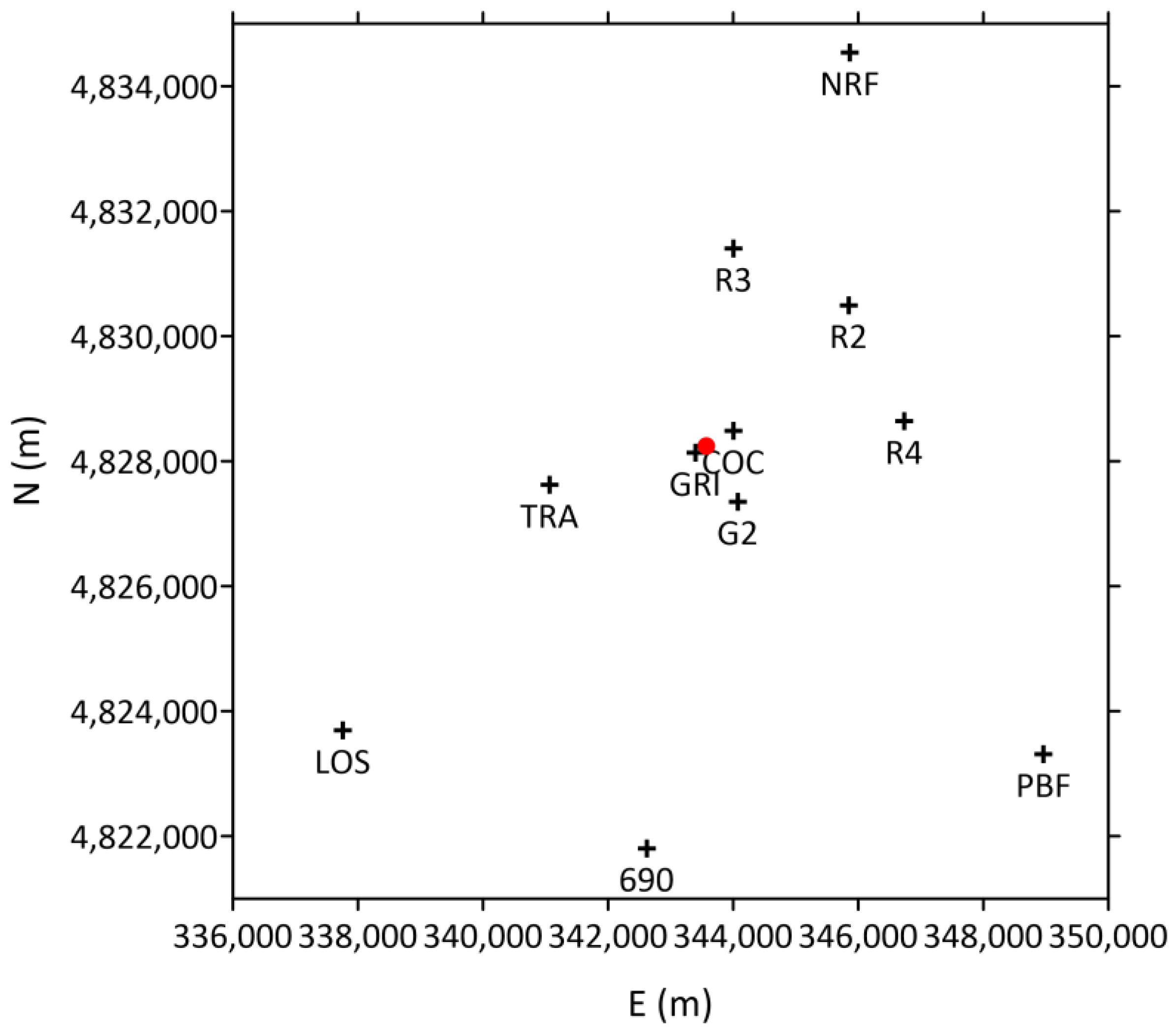
Atmosphere 16 00671 g001
Figure 2. CALMET domain, position of the source (red circle) and of the meteorological stations used in the model (black plus).
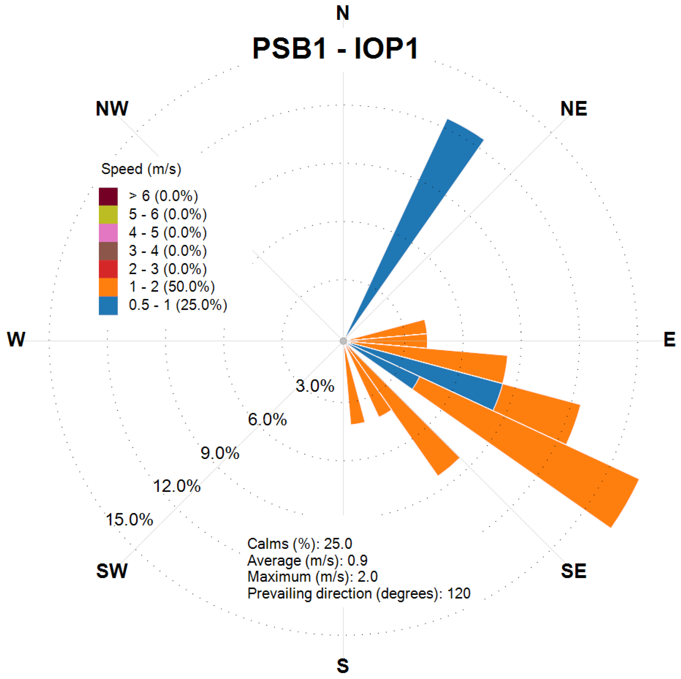
Atmosphere 16 00671 g002
Figure 3. Wind rose obtained from the CALMET output at the release location for the final 2 h of PSB1-IOP1.
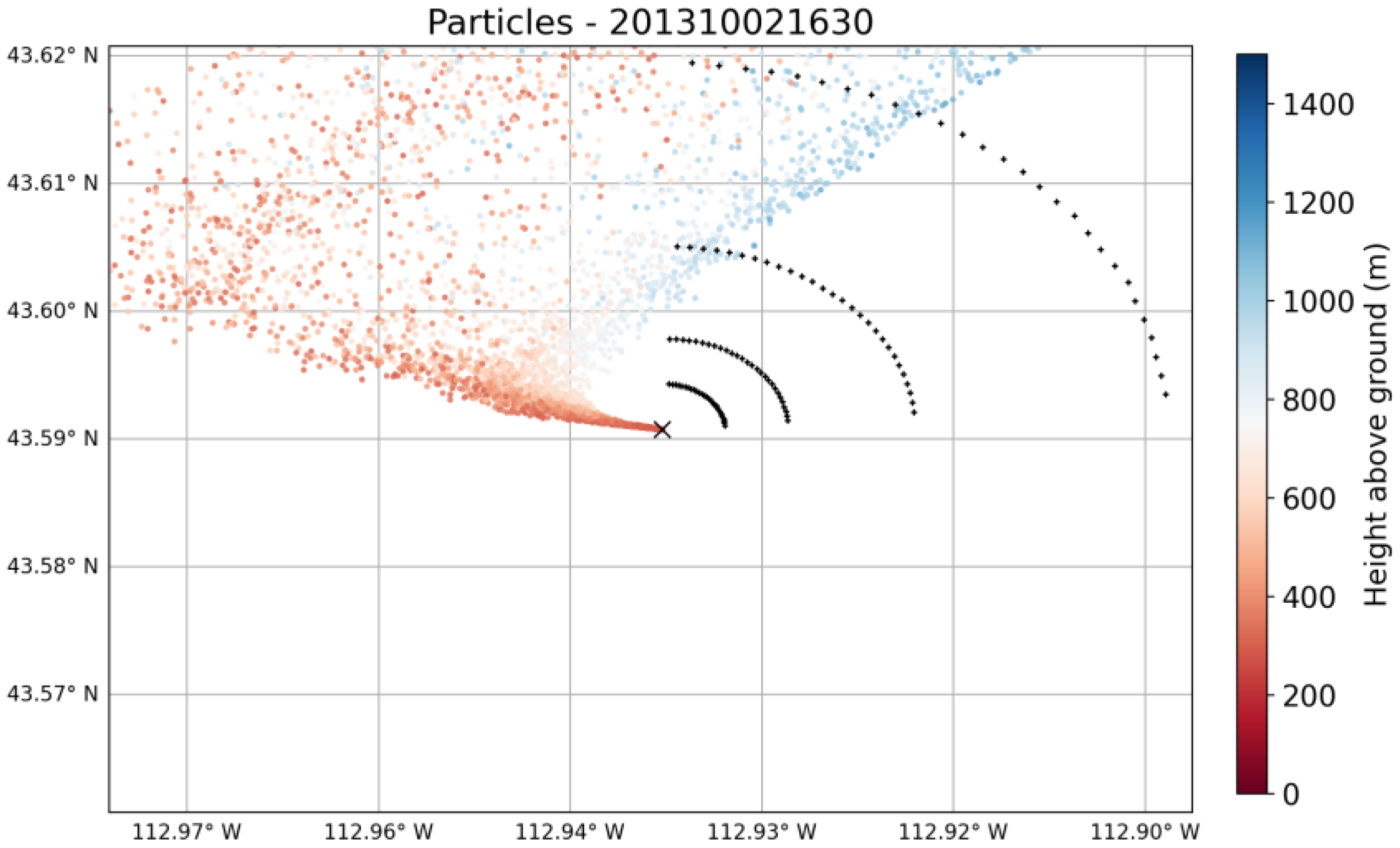
Atmosphere 16 00671 g003
Figure 4. Computational particles (dots with different colors according to their height agl) of LAPMOD at 16:30 MST of 2 October 2013 (PSB1-IOP1). Sampling locations are represented by black crosses, while the source is represented by a black ×.
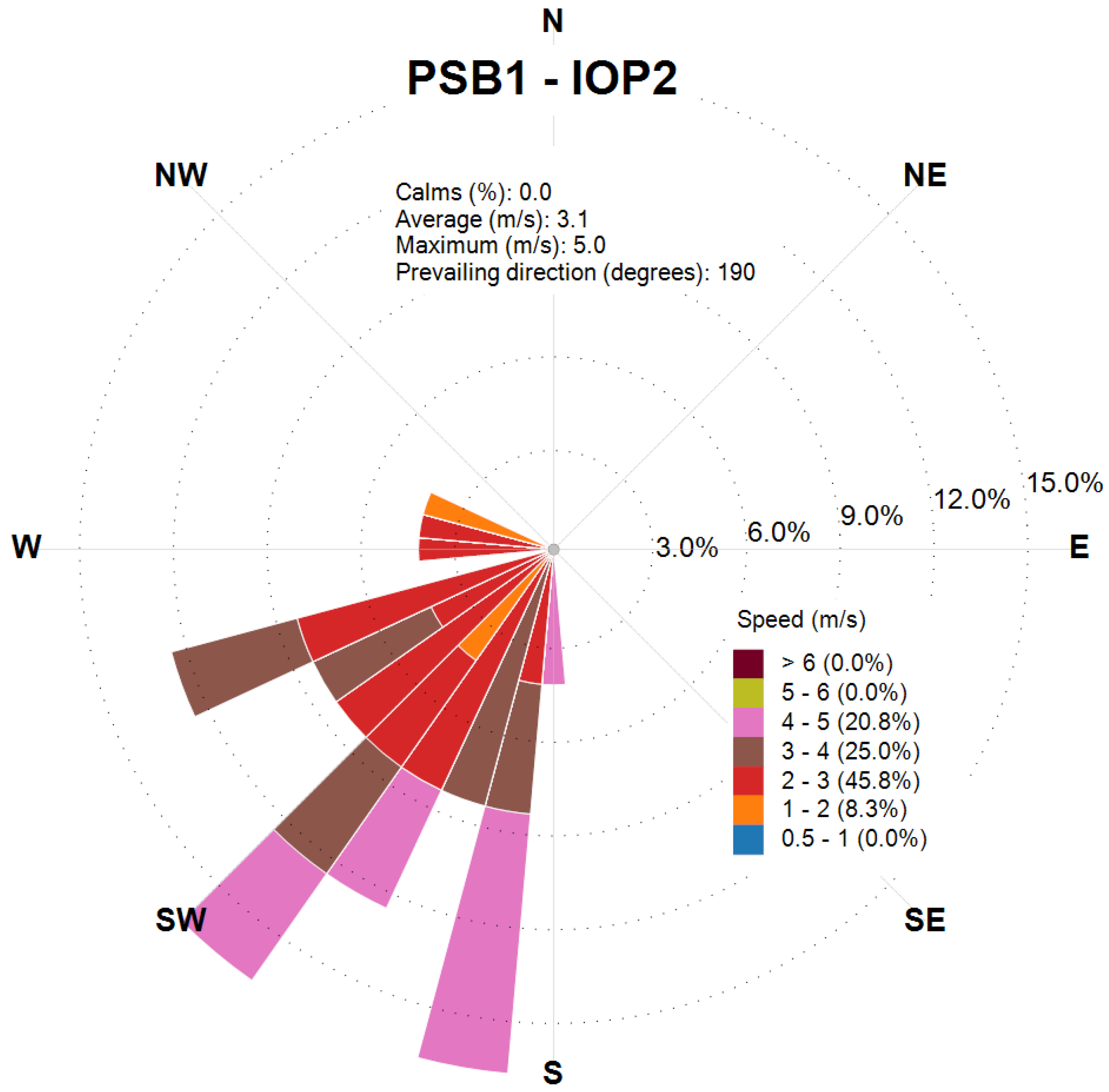
Atmosphere 16 00671 g004
Figure 5. Wind rose obtained from the CALMET output at the release location for the final 2 h of PSB1-IOP2.
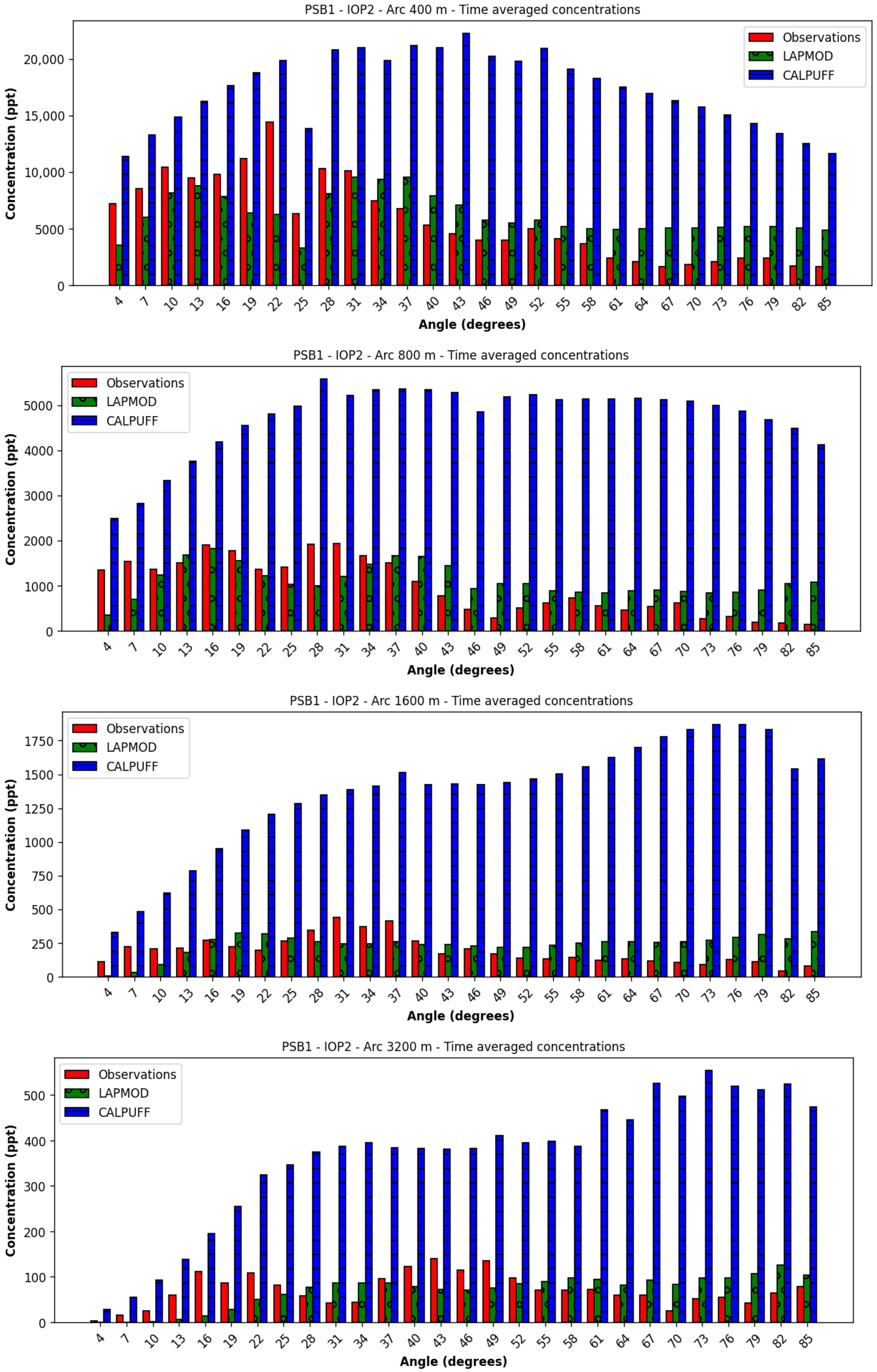
Atmosphere 16 00671 g005
Figure 6. Time-averaged concentrations at the arcs of PSB1-IOP2.
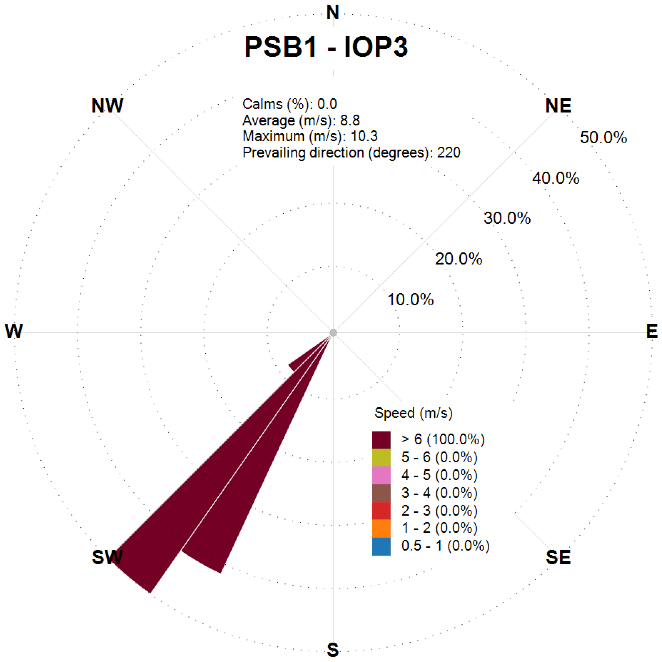
Atmosphere 16 00671 g006
Figure 7. Wind rose obtained from the CALMET output at the release location for the final 2 h of PSB1-IOP3.
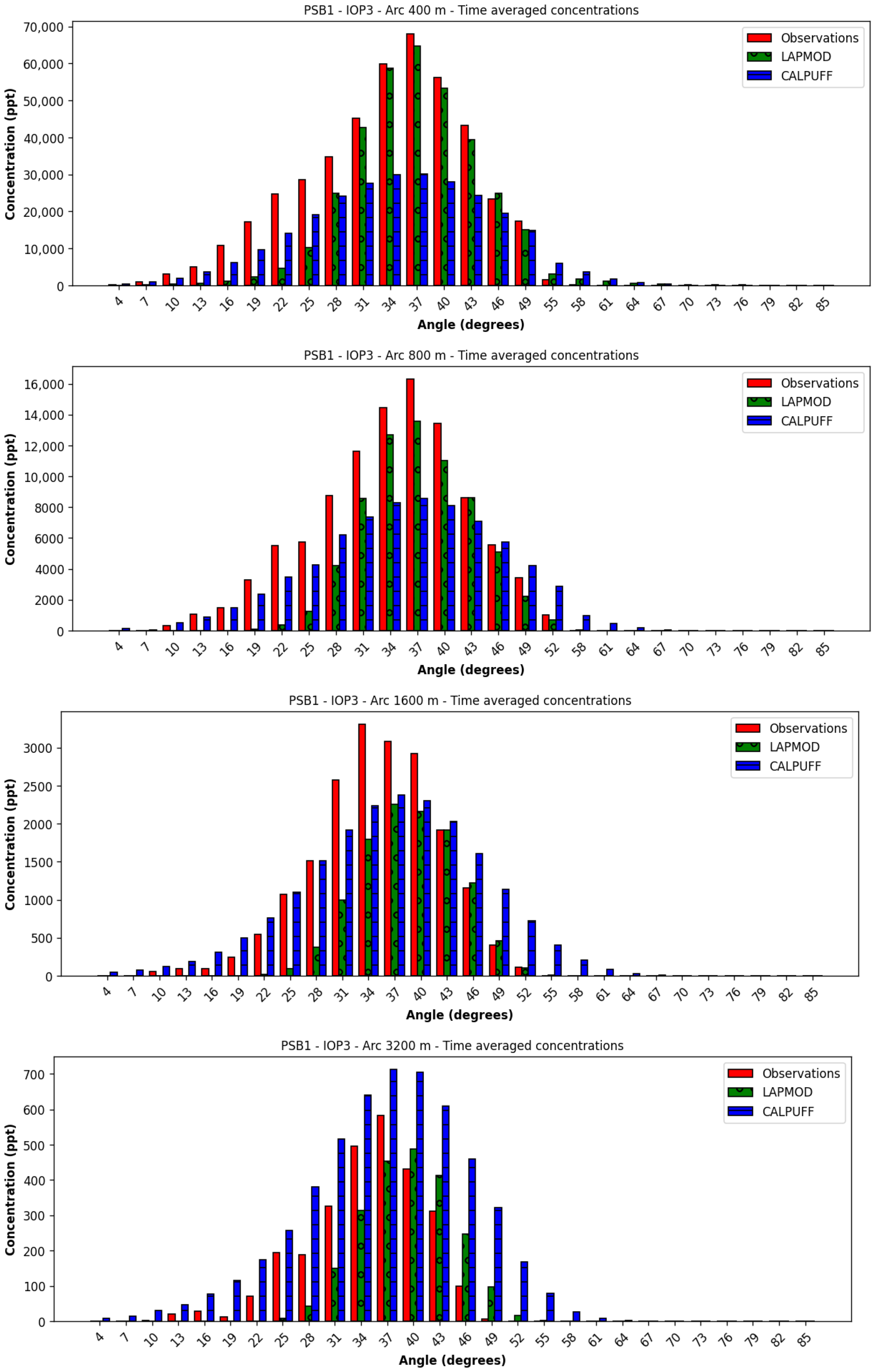
Atmosphere 16 00671 g007
Figure 8. Time-averaged concentrations at the arcs of PSB1-IOP3.
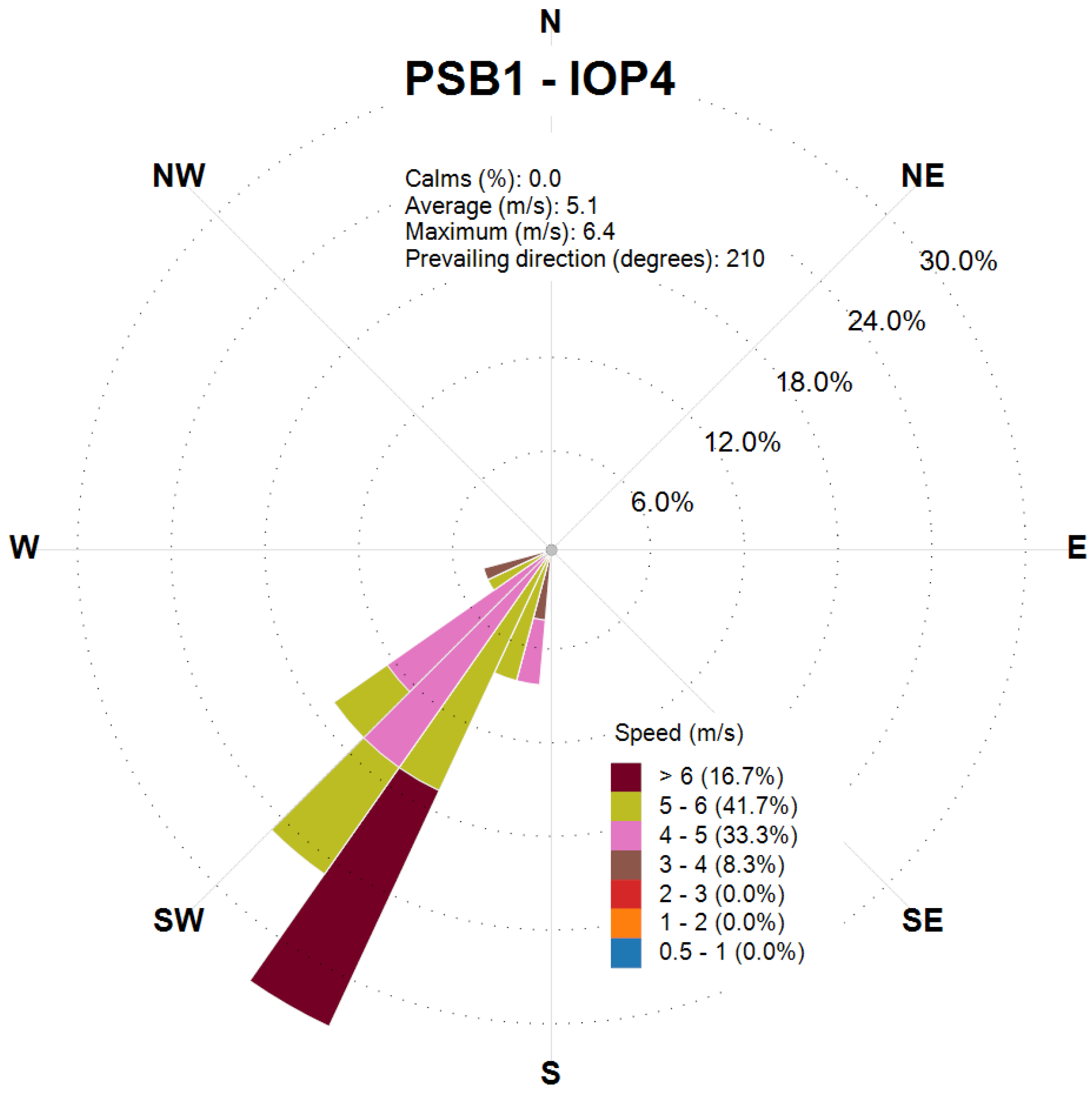
Atmosphere 16 00671 g008
Figure 9. Wind rose obtained from the CALMET output at the release location for the final 2 h of PSB1-IOP4.
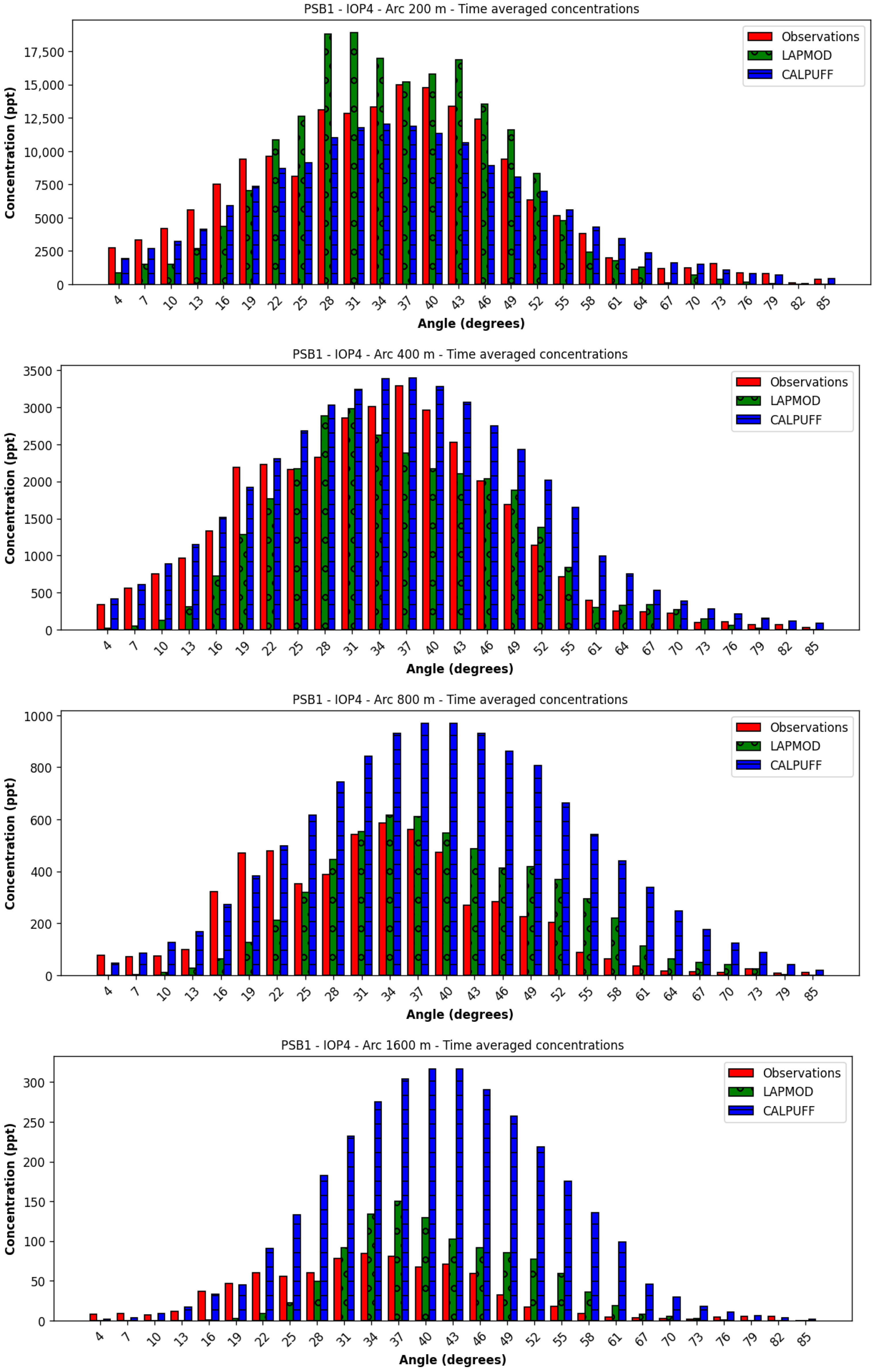
Atmosphere 16 00671 g009
Figure 10. Time-averaged concentrations at the arcs of PSB1-IOP4.
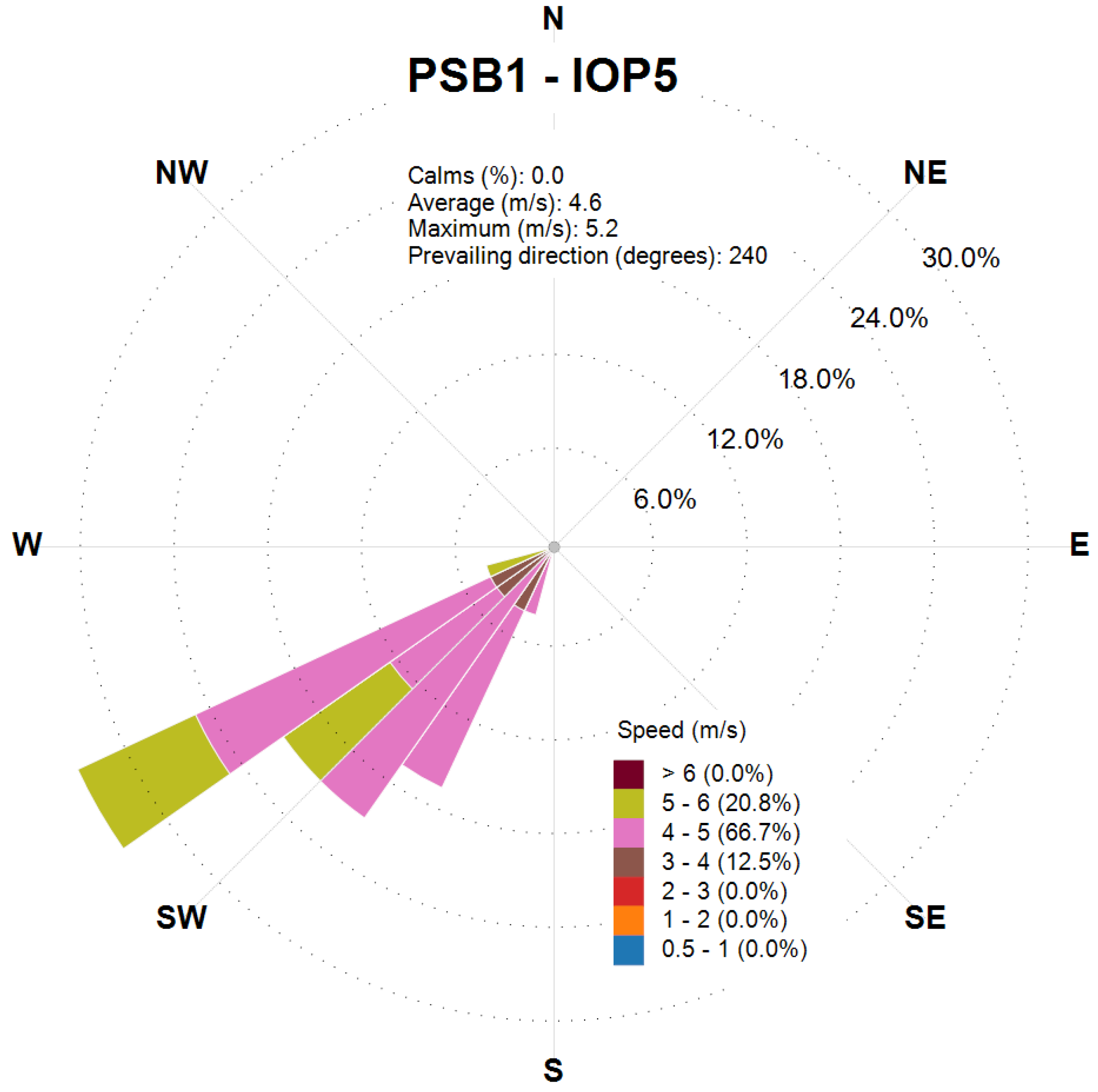
Atmosphere 16 00671 g010
Figure 11. Wind rose obtained from the CALMET output at the release location for the final 2 h of PSB1-IOP5.
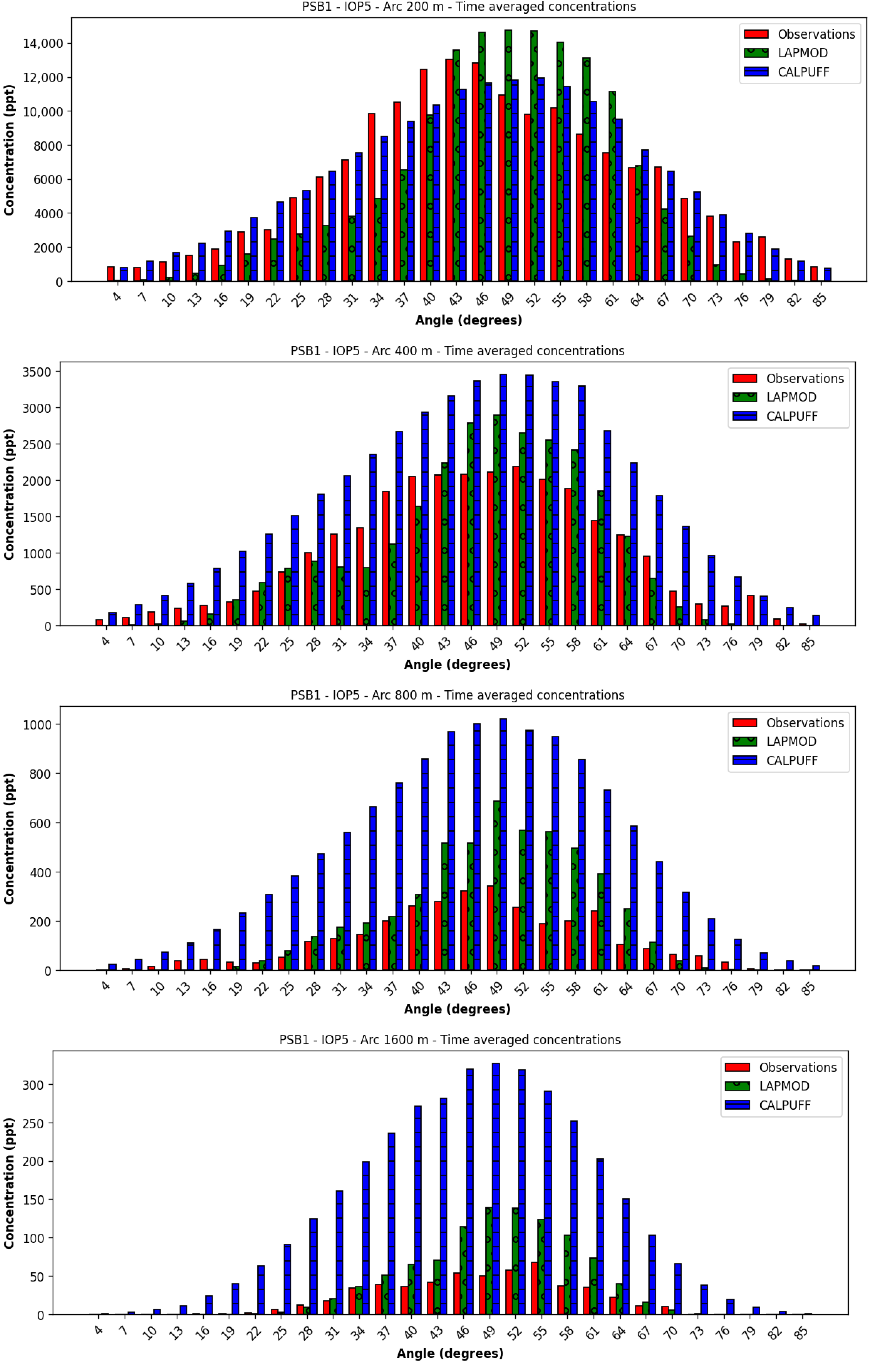
Atmosphere 16 00671 g011
Figure 12. Time-averaged concentrations at the arcs of PSB1-IOP5.
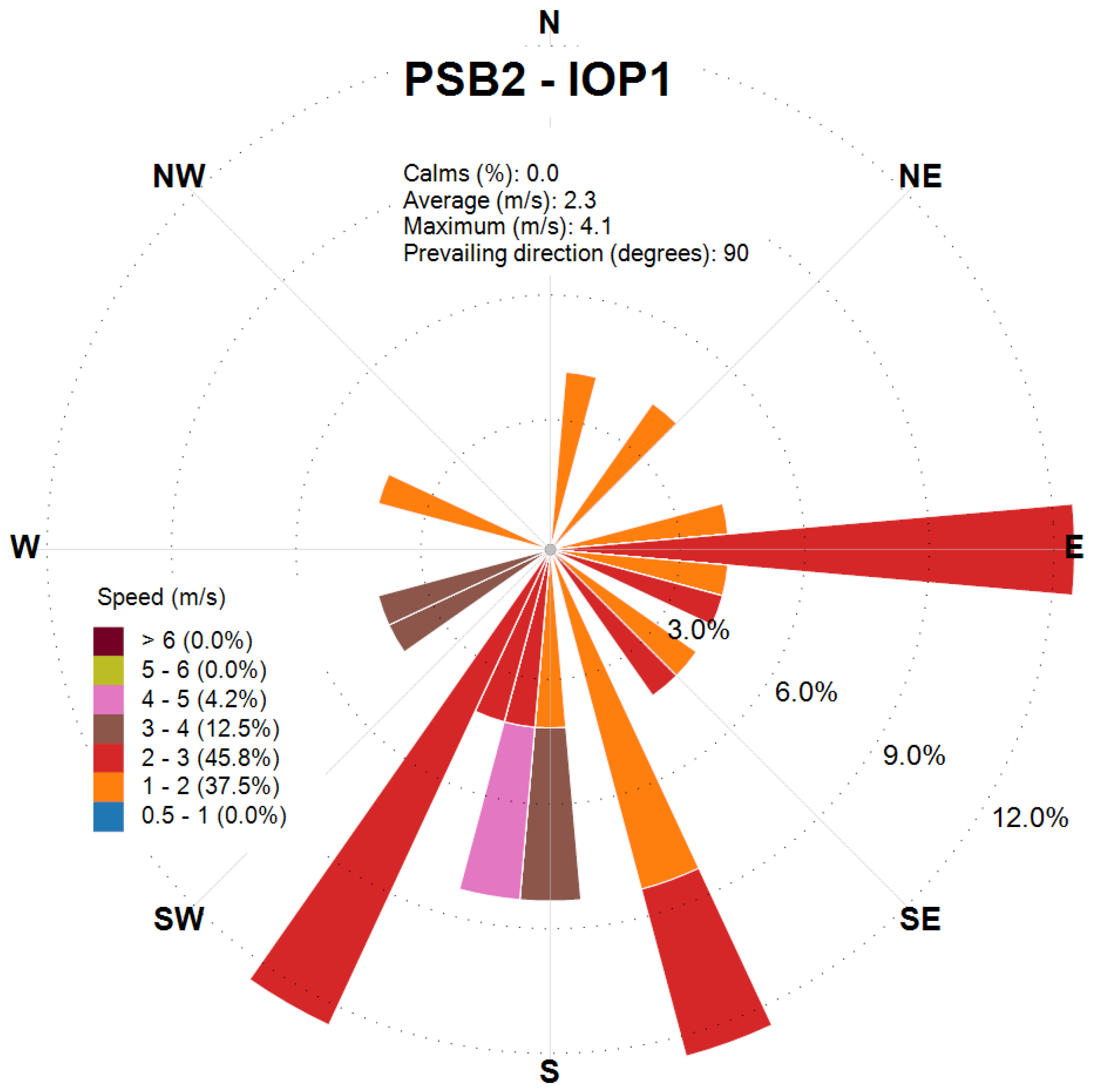
Atmosphere 16 00671 g012
Figure 13. Wind rose obtained from the CALMET output at the release location for the final 2 h of PSB2-IOP1.
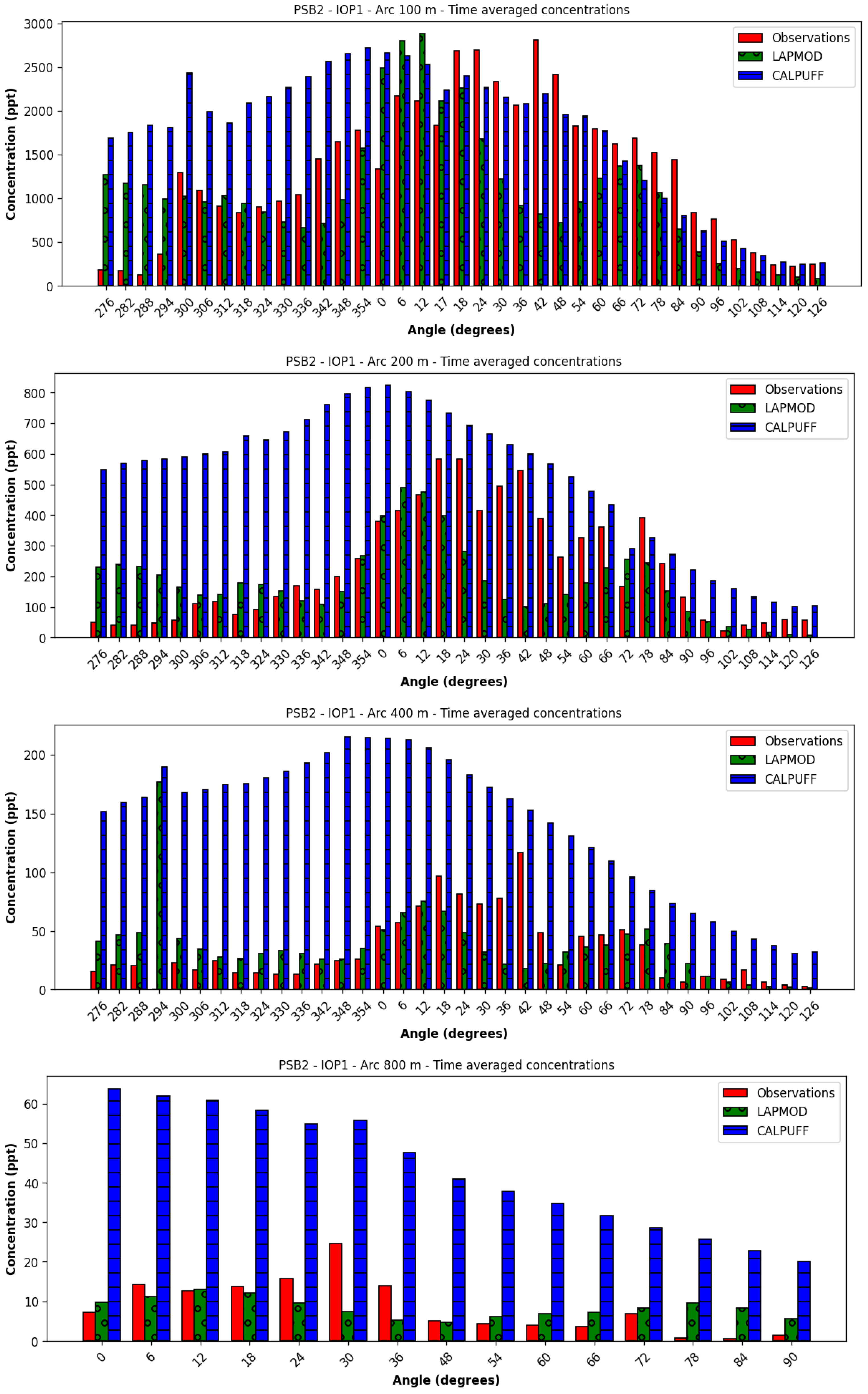
Atmosphere 16 00671 g013
Figure 14. Time-averaged concentrations at the arcs of PSB2-IOP1.
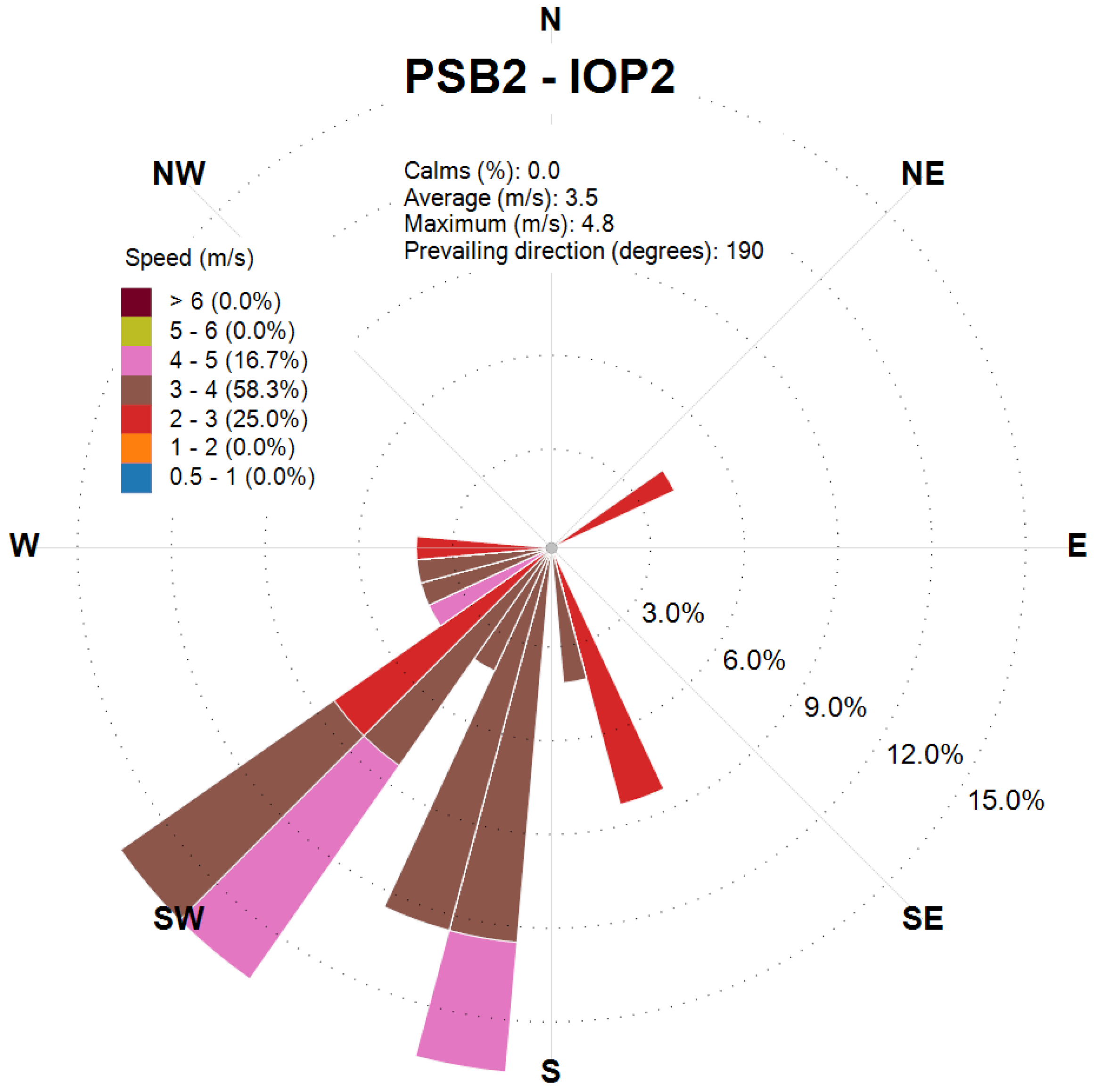
Atmosphere 16 00671 g014
Figure 15. Wind rose obtained from the CALMET output at the release location for the final 2 h of PSB2-IOP2.
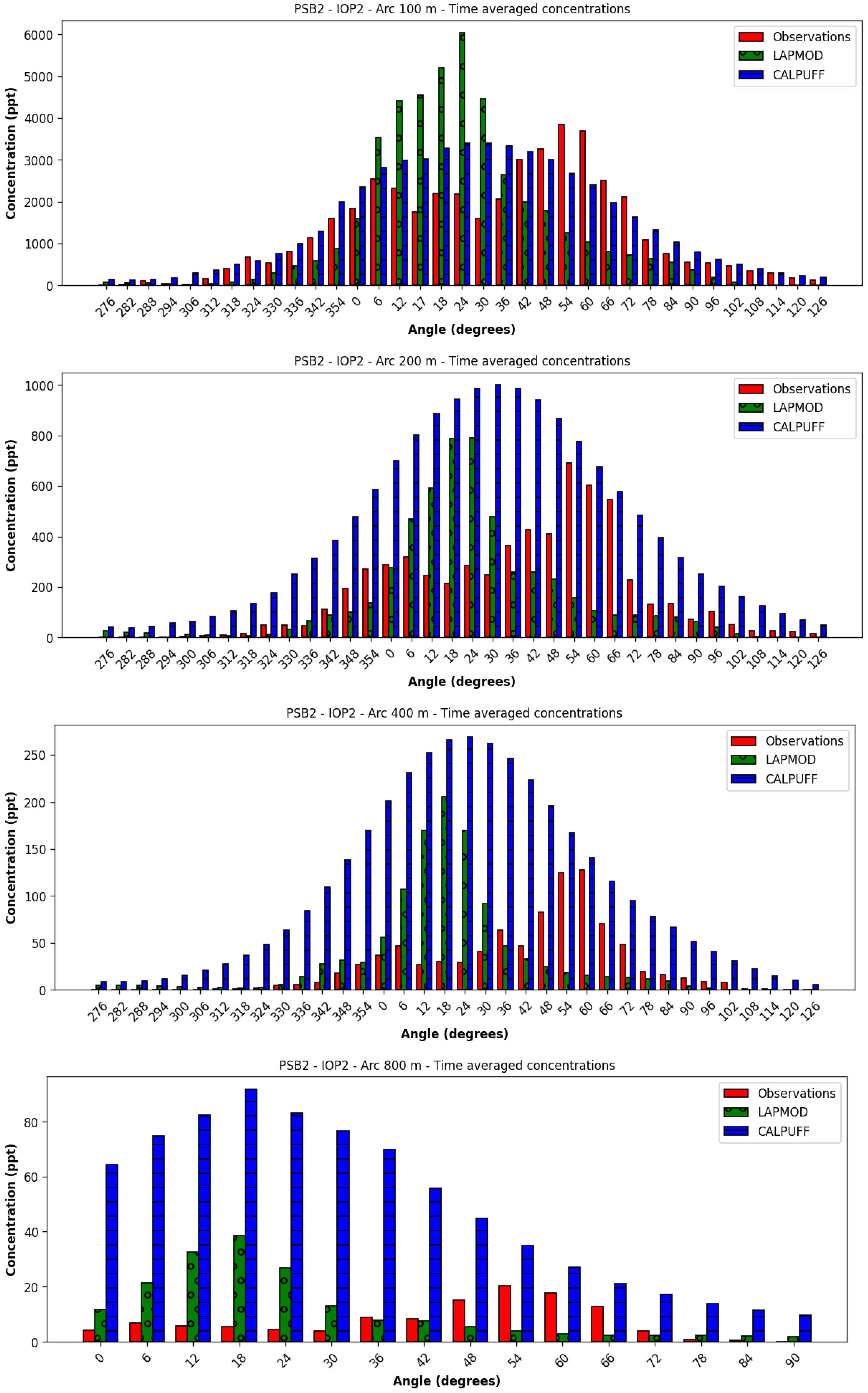
Atmosphere 16 00671 g015
Figure 16. Time-averaged concentrations at the arcs of PSB2-IOP2.
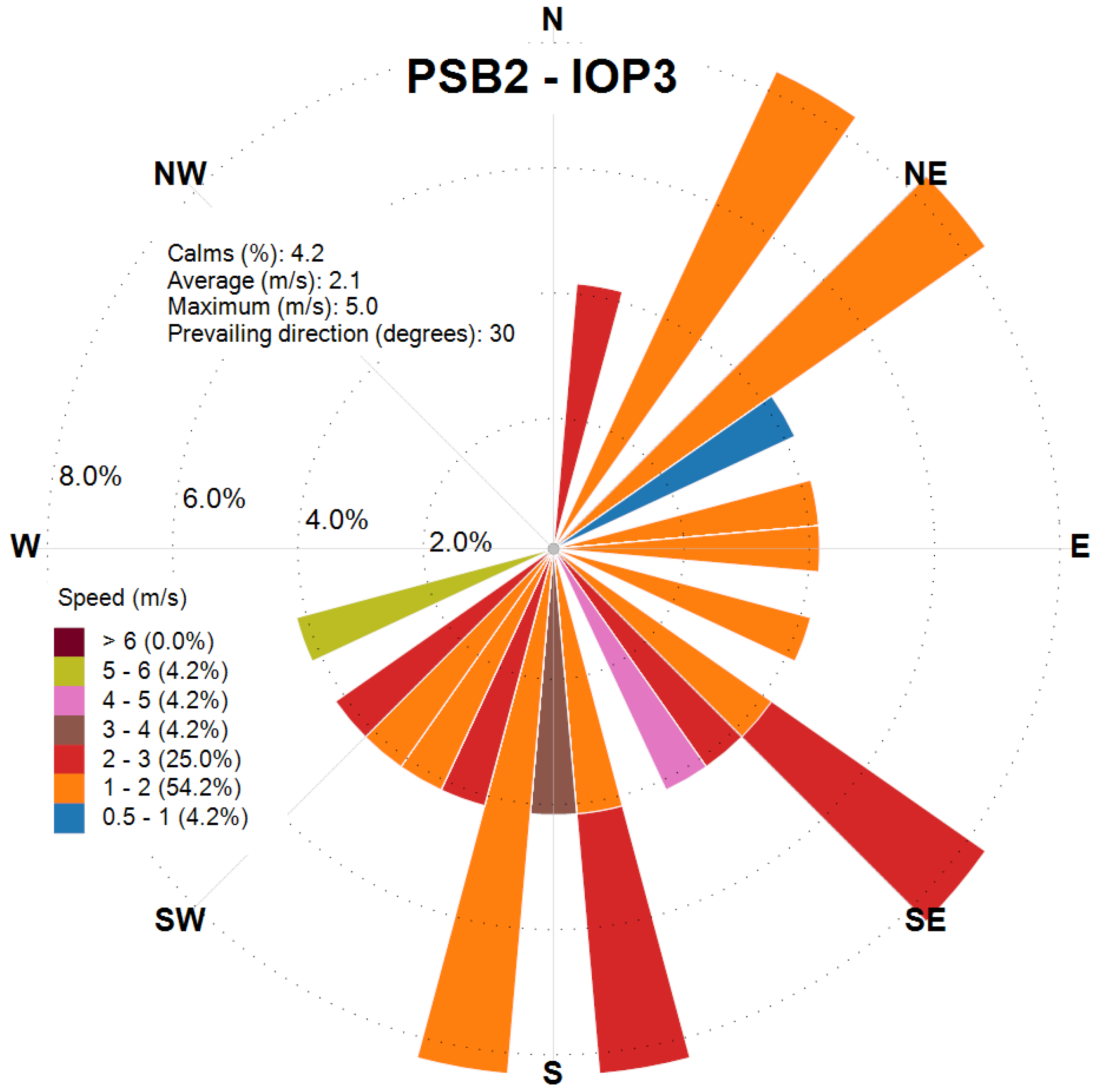
Atmosphere 16 00671 g016
Figure 17. Wind rose obtained from the CALMET output at the release location for the final 2 h of PSB2-IOP3.
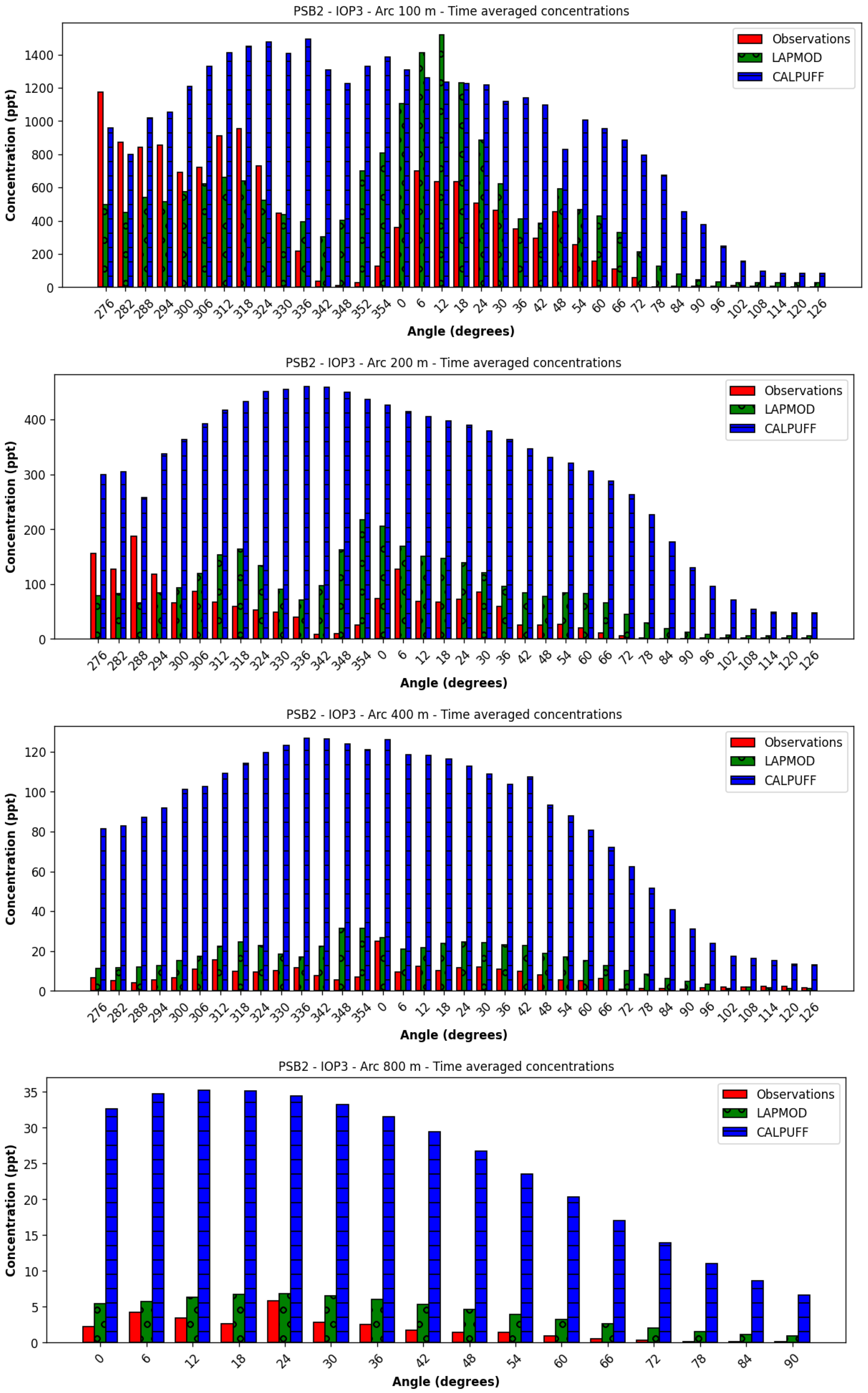
Atmosphere 16 00671 g017
Figure 18. Time-averaged concentrations at the arcs of PSB2-IOP3.
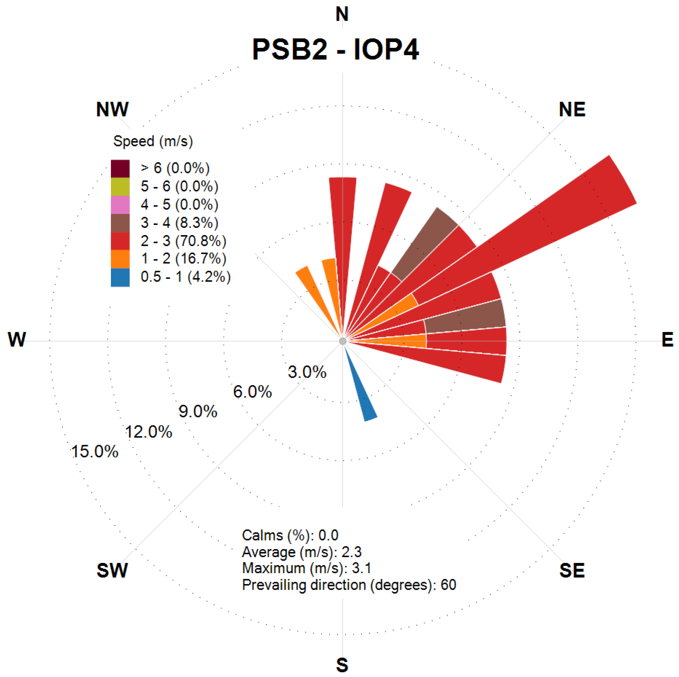
Atmosphere 16 00671 g018
Figure 19. Wind rose obtained from the CALMET output at the release location for the final 2 h of PSB2-IOP4.
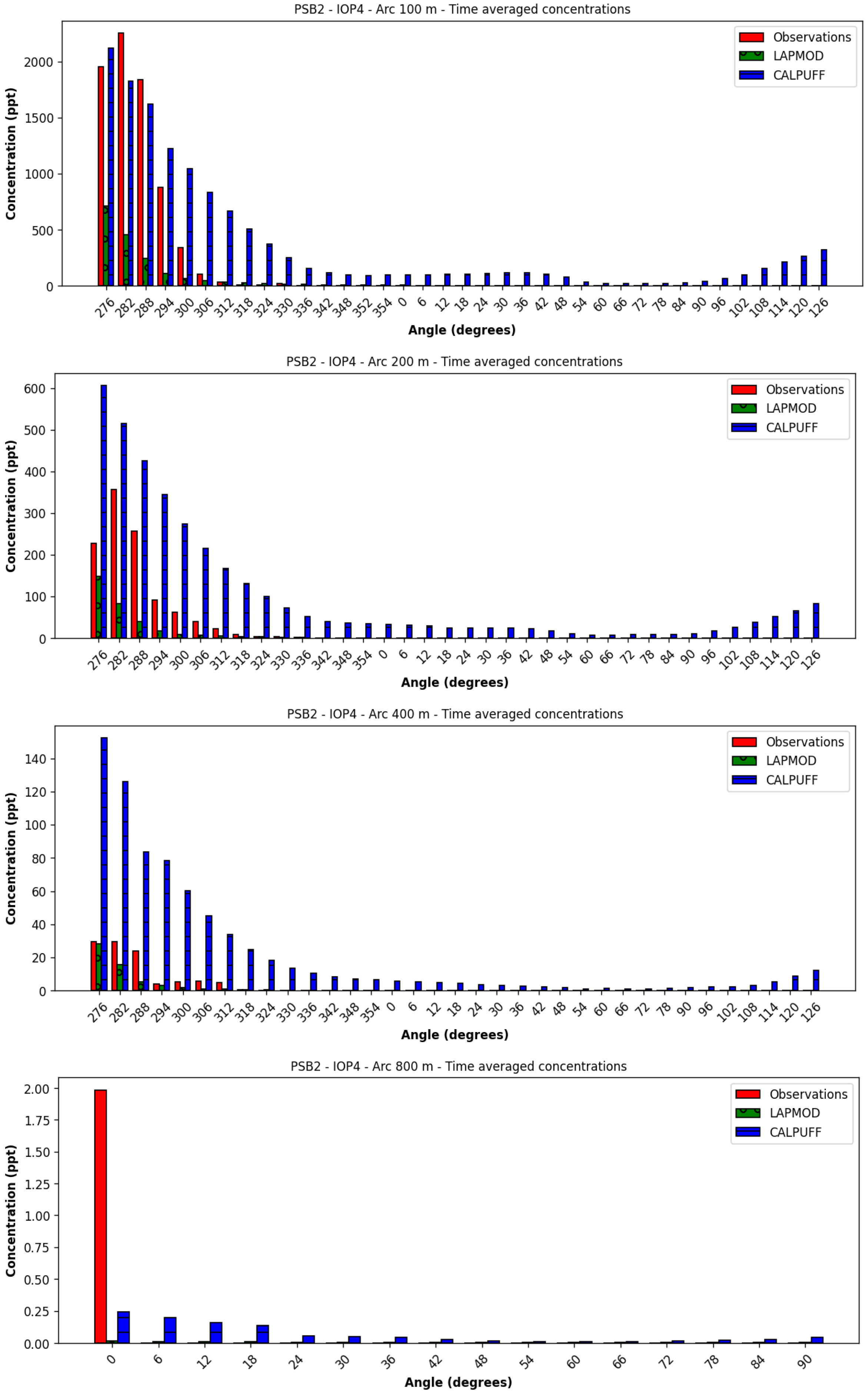
Atmosphere 16 00671 g019
Figure 20. Time-averaged concentrations at the arcs of PSB2-IOP4.
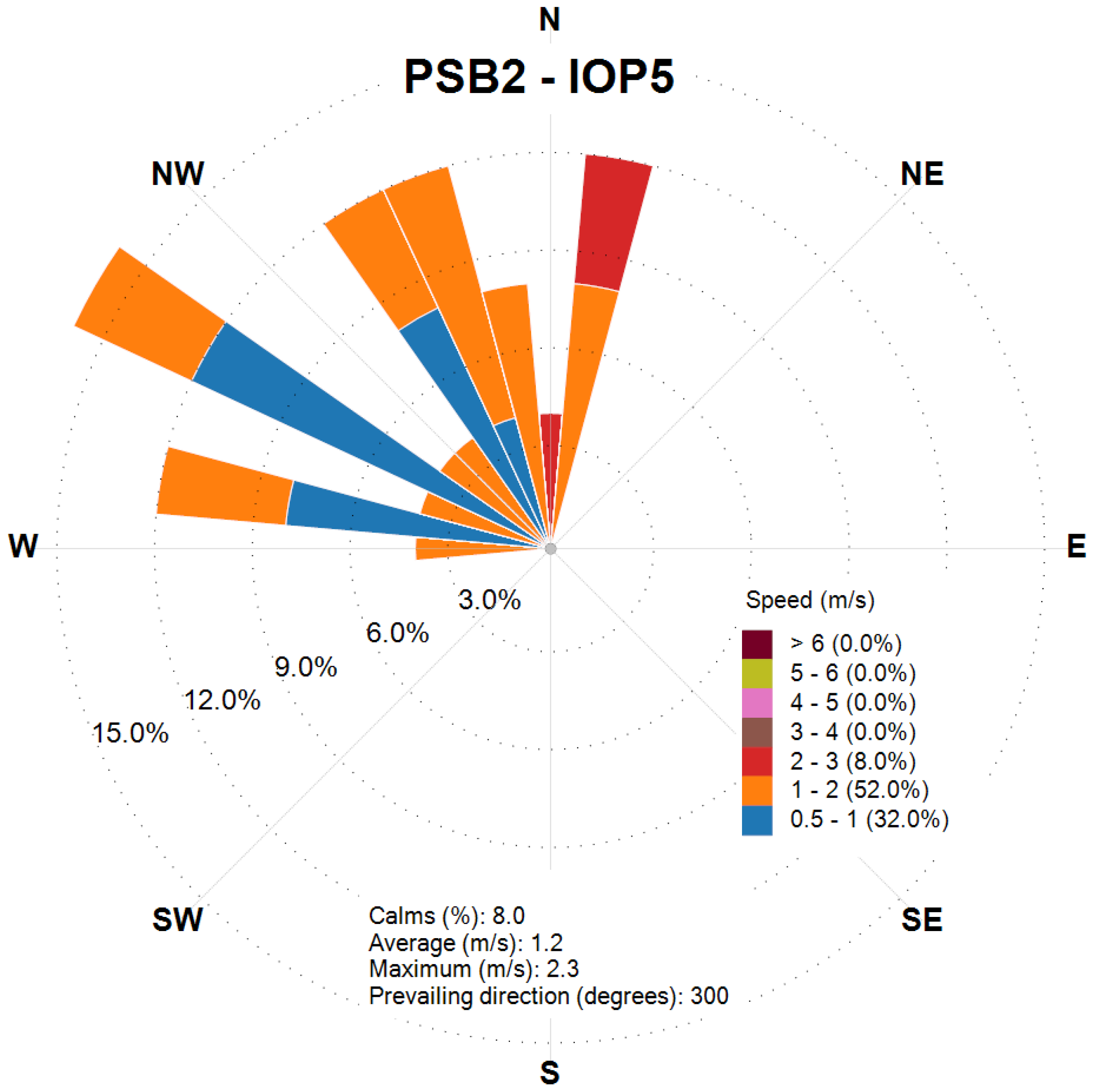
Atmosphere 16 00671 g020
Figure 21. Wind rose obtained from the CALMET output at the release location for the final 2 h of PSB2-IOP5.
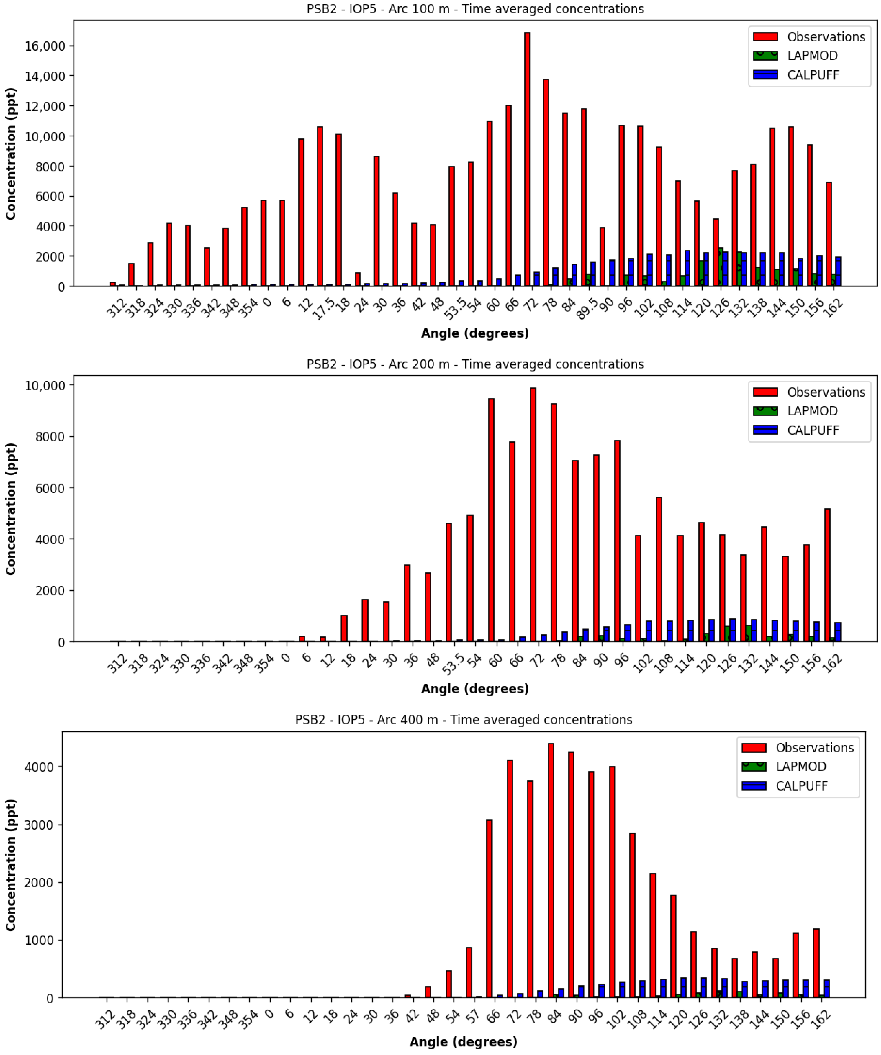
Atmosphere 16 00671 g021
Figure 22. Time-averaged concentrations at the arcs of PSB2-IOP5.
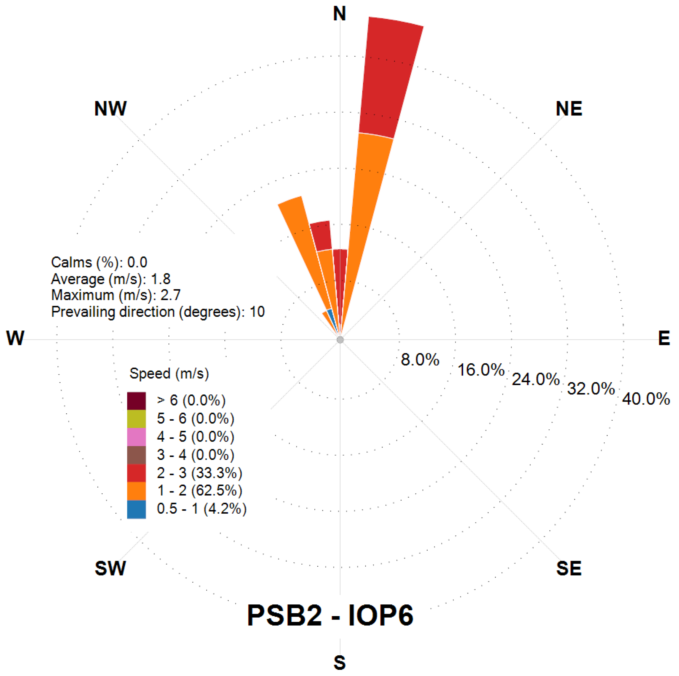
Atmosphere 16 00671 g022
Figure 23. Wind rose obtained from the CALMET output at the release location for the final 2 h of PSB2-IOP6.
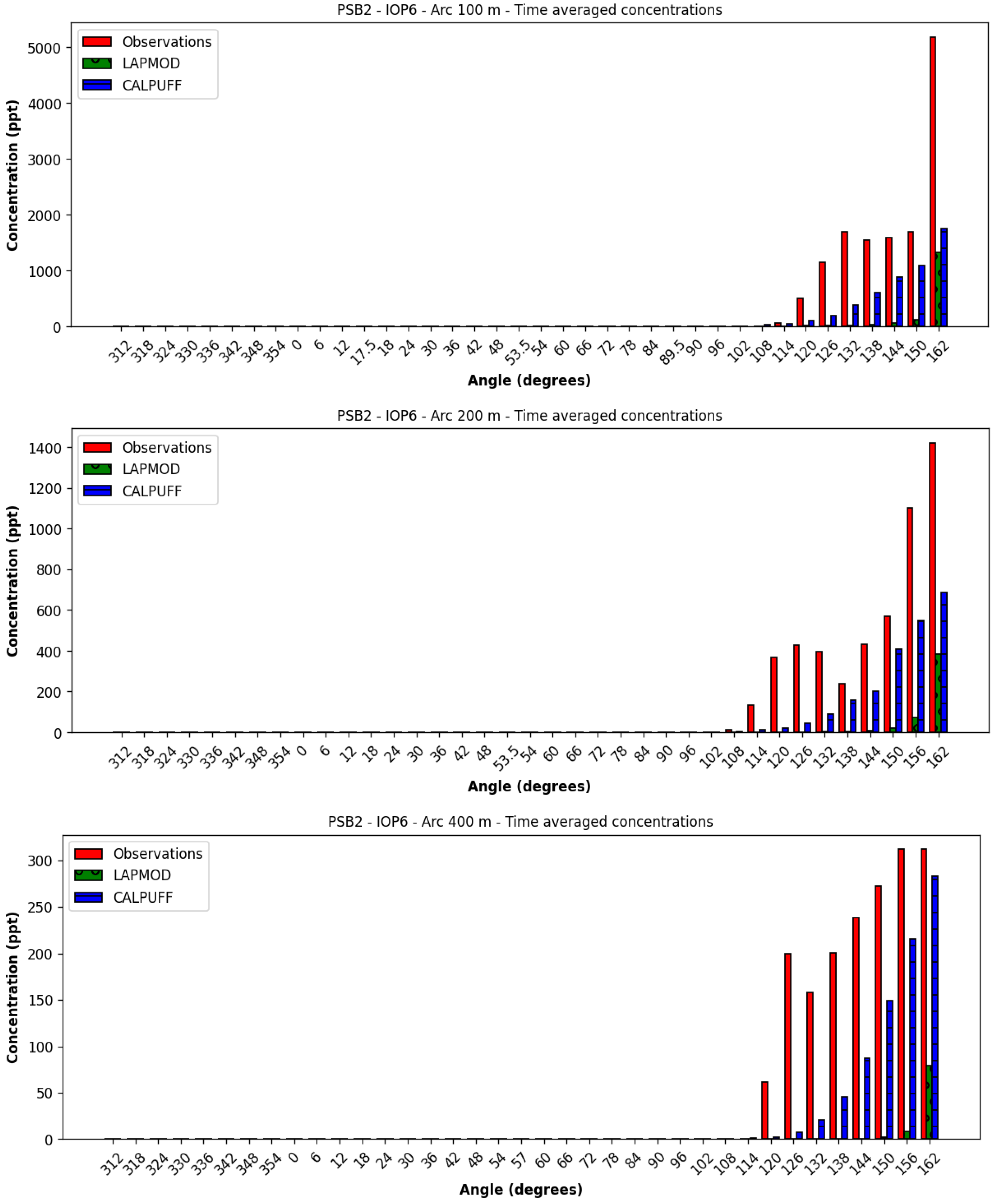
Atmosphere 16 00671 g023
Figure 24. Time-averaged concentrations at the arcs of PSB2-IOP6.
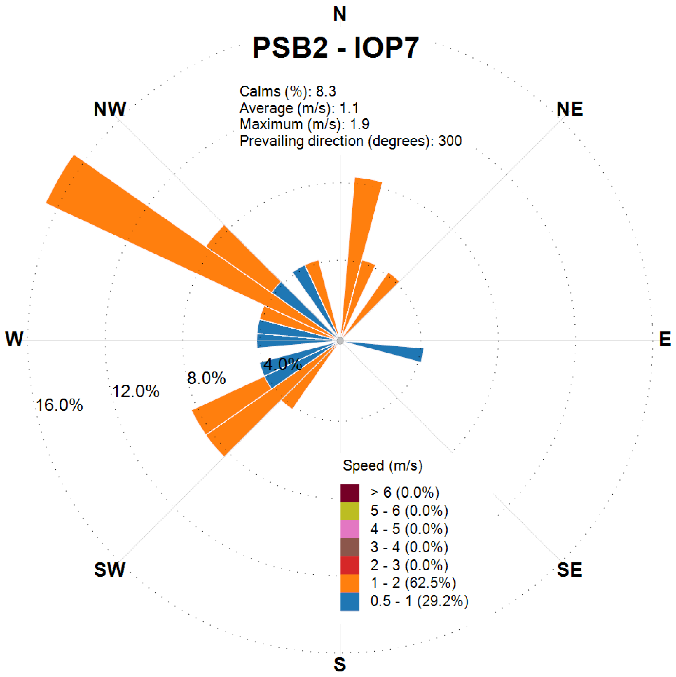
Atmosphere 16 00671 g024
Figure 25. Wind rose obtained from the CALMET output at the release location for the final 2 h of PSB2-IOP7.
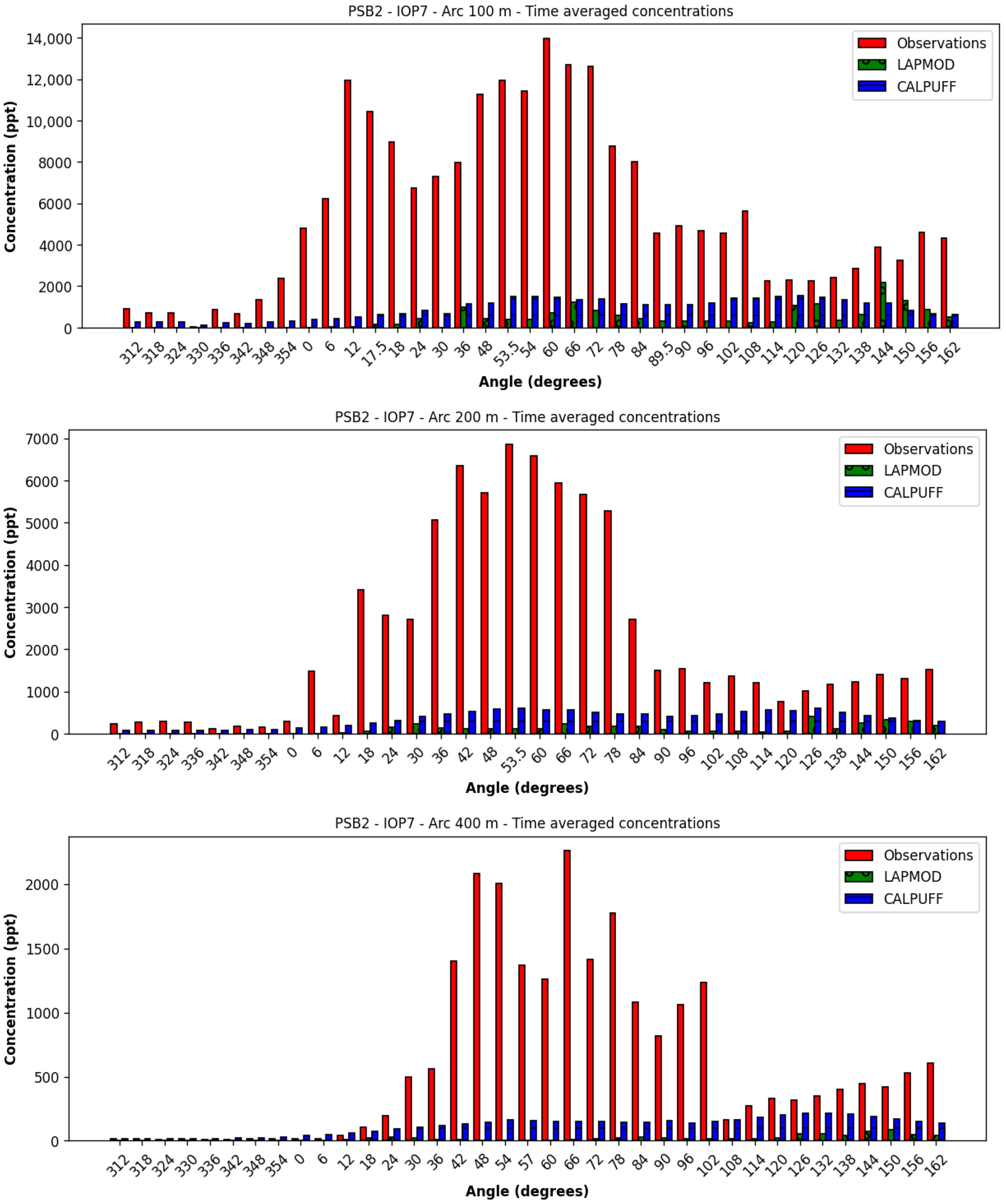
Atmosphere 16 00671 g025
Figure 26. Time-averaged concentrations at the arcs of PSB2-IOP7.
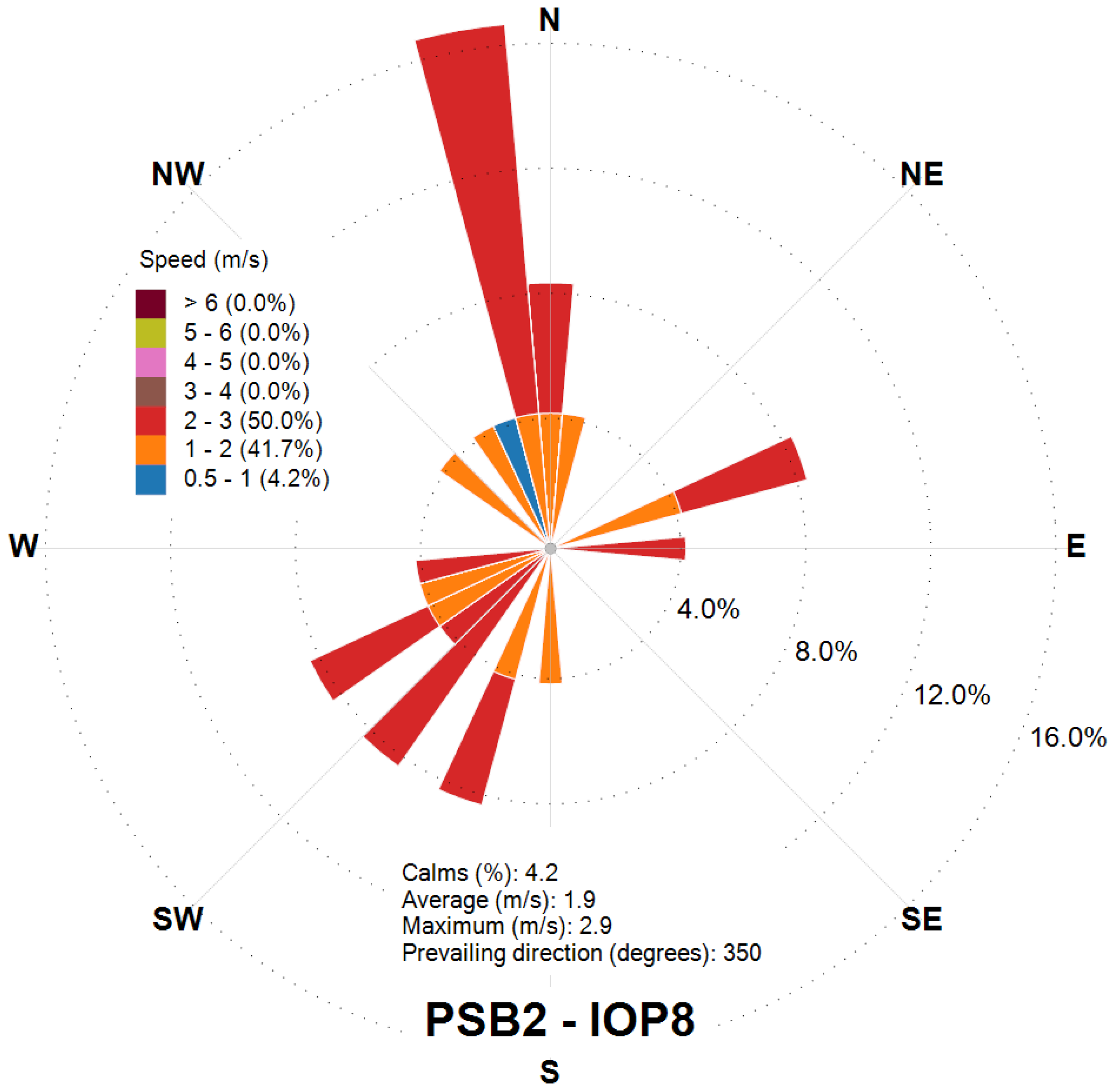
Atmosphere 16 00671 g026
Figure 27. Wind rose obtained from the CALMET output at the release location for the final 2 h of PSB2-IOP8.
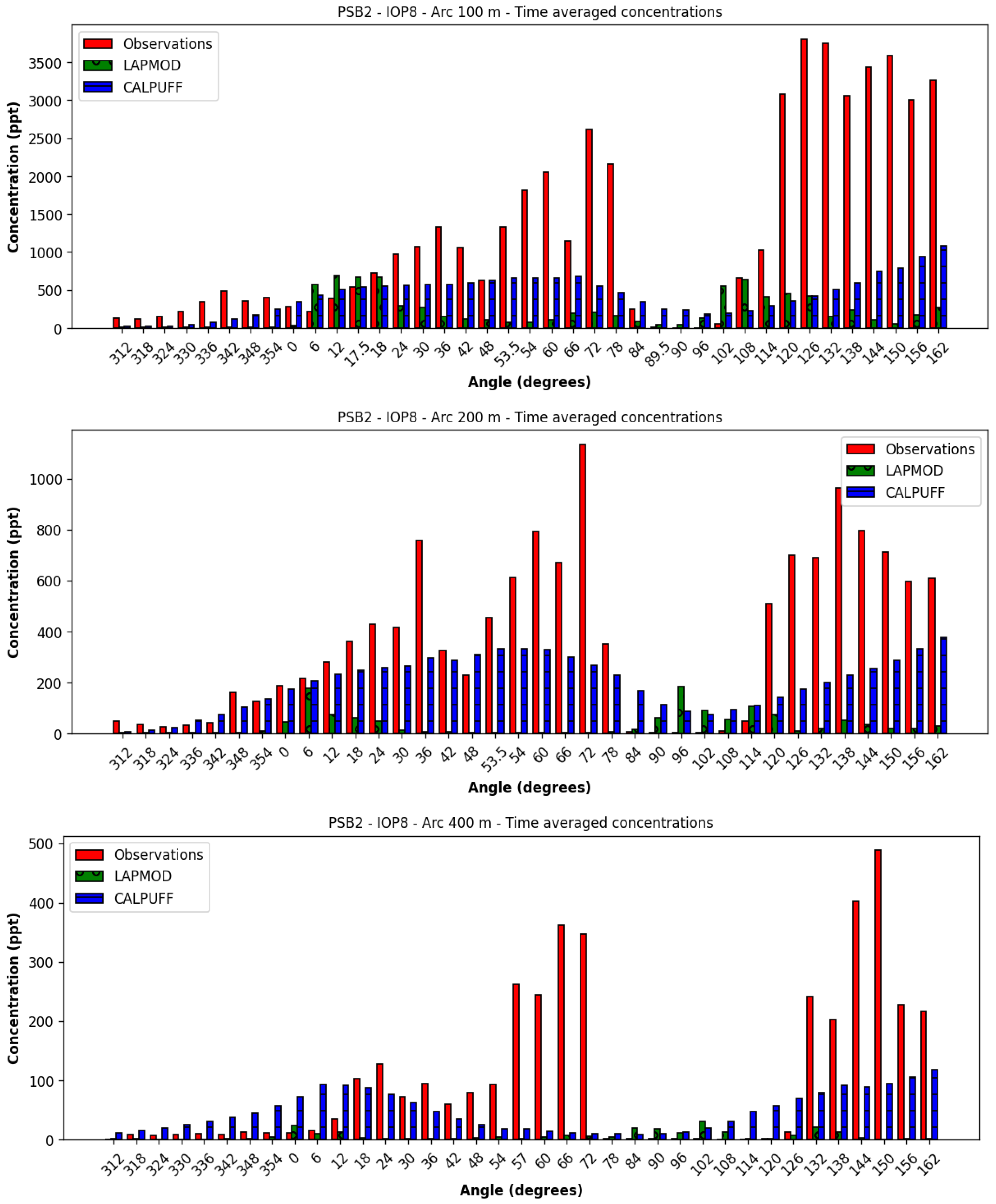
Atmosphere 16 00671 g027
Figure 28. Time-averaged concentrations at the arcs of PSB2-IOP8.
Atmosphere 16 00671 g028
Table 1. PSB1 release information. Each release lasted 2.5 h.
IOPDate (2013)Start Time (MST)Release Rate (g/s)Temperature (°C)
12 October14:0010.17716.5
25 October12:309.98616.8
37 October12:309.93024.9
411 October13:301.04317.1
518 October12:301.03015.6
Table 2. PSB2 release information. Each release lasted 2.5 h.
IOPDate (2016)Start Time (MST)Release Rate (g/s)Temperature (°C)
126 July11:300.192237.0
227 July11:000.146036.5
34 August12:300.121832.6
45 August12:000.146632.1
513 October03:300.014713.5
620 October03:300.012012.9
721 October03:300.012012.3
826 October18:000.011921.4
Table 3. CALPUFF input variables.
VariableDescriptionValue
NSECDTLength of modeling time-step (s)300
MGAUSSVertical distribution used in the near field (0: Uniform; 1: Gaussian)1
MCTADJTerrain adjustment method (3: Partial plume path adjustment)3
MRISEPlume rise method (0: Briggs; 1 Numerical)1
MWETWet removal (0: Not modeled; 1: Modeled)0
MDRYDry removal (0: Not modeled; 1: Modeled)0
MDISPMethod to compute dispersion coefficients2
MPARTLPartial plume penetration of elevated inversion modeled (0: No; 1: Yes)1
MPDFPDF used for dispersion under convective conditions (0: No; 1: Yes)0
MDISP = 2 means that dispersion coefficients are obtained from internally calculated sigma v, sigma w using micrometeorological variables.
Table 4. LAPMOD input variables.
VariableDescriptionValue
LDEPDActivation of dry depositionFalse
LDEPWActivation of wet depositionFalse
ITDMQTime step (s) to query meteorological variables at particle’s position (0 to interpolate at any timestep)0
LNOWSuppress the vertical component of the CALMET wind speedFalse
NPARTParticles released every 60 s120
IPRTYPEPlume rise type (1 for Janicke and Janicke; 2 for Webster and Thomson)2
LSTDActivate stack tip downwashFalse
LPPPActivate partial plume penetrationTrue
LPITActivate plume-induced turbulenceTrue
IDTORDTime step to write concentrations (s)600
NSAMNumber of samplings to get average concentrations over IDTORD2
CCAAlgorithm for calculating concentrations (1: Gaussian kernel; 2: Uliasz uniform kernel; 3: Uliasz parabolic kernel)1
SIGNUMNumber of sigma units defining the volume associated with each particle and for searching contributing particles3
Table 5. Equivalence between cloud cover category and cloud cover in tenths.
ASOS Cloud CoverDescriptionCloud Cover (Tenths)
CLRClear0
FEWFew1
SCTScattered3
BKNBroken7
OVCOvercast10
Table 6. UTM12T Coordinates and anemometer height of the surface stations used in CALMET.
IDE (m)N (m)H agl (m)Description
10002343,3984,828,1342.0GRI at 2 m agl
12001342,6184,821,80515.0Central Facilities (690)
12002337,7564,823,69215.0Lost River Rest Area (LOS)
12003345,8674,834,54015.0Naval Reactors Facility (NRF)
12004348,9634,823,31215.0Critical Infrastructure Complex (PBF)
12005341,0664,827,62115.0Reactor Technologies Complex (TRA)
11002344,0024,828,4862.0COC at 2 m agl
13002345,8474,830,4953.2Sonic anemometer R2
13003344,0054,831,4033.2Sonic anemometer R3
13004346,7364,828,6423.2Sonic anemometer R4
14003344,0774,827,3523.1Sonic anemometer G2
Table 7. Statistical parameters for PSB1-IOP2.
StatisticsPaired400 m arc800 m arc1600 m arc3200 m arc
N148928282828
Max Obs (ppt)62,48414,4291936438140
Max LAPMOD (ppt)121,92095681816335126
Max CALPUFF (ppt)121,72222,26355831870554
FA2 LAPMOD27.560.767.960.764.3
FA5 LAPMOD42.3100.092.989.382.1
FA2 CALPUFF22.225.07.10.03.6
FA5 CALPUFF40.864.346.439.346.4
Corr. LAPMOD0.420.560.47−0.030.19
Corr. CALPUFF0.720.30−0.20−0.240.23
FB LAPMOD0.250.080.140.21−0.02
FB CALPUFF1.121.001.321.501.35
FMS LAPMOD68.9100.0100.0100.092.6
FMS CALPUFF81.2100.0100.0100.096.4
NMSE LAPMOD13.260.250.290.400.40
NMSE CALPUFF8.431.503.375.934.07
FOEX LAPMOD−10.014.314.317.90.0
FOEX CALPUFF32.450.050.050.050.0
Rank LAPMOD3.24.24.03.43.9
Rank CALPUFF2.72.41.61.42.0
Table 8. Statistical parameters for PSB1-IOP3.
StatisticsPaired400 m arc800 m arc1600 m arc3200 m arc
N148827272828
Max Obs188,92167,98916,3073309583
Max LAPMOD129,85664,60513,5502257487
Max CALPUFF71,32930,05585452377713
FA2 LAPMOD47.633.344.453.650.0
FA5 LAPMOD58.740.751.960.760.7
FA2 CALPUFF44.963.066.750.046.4
FA5 CALPUFF57.677.870.467.964.3
Corr. LAPMOD0.730.960.950.920.88
Corr. CALPUFF0.830.970.960.950.92
FB LAPMOD−0.24−0.23−0.38−0.50−0.22
FB CALPUFF−0.29−0.49−0.310.030.63
FMS LAPMOD63.766.772.268.864.3
FMS CALPUFF58.778.372.771.465.0
NMSE LAPMOD5.780.220.431.120.85
NMSE CALPUFF4.940.980.610.301.07
FOEX LAPMOD−15.5−5.6−24.1−32.1−21.4
FOEX CALPUFF2.6−16.7−5.614.325.0
Rank LAPMOD3.53.83.53.33.6
Rank CALPUFF3.84.04.14.03.4
Table 9. Statistical parameters for PSB1-IOP4.
StatisticsPaired200 m arc400 m arc800 m arc1600 m arc
N146428272627
Max Obs48,66914,993328758784
Max LAPMOD56,05218,9172982617150
Max CALPUFF18,15212,0153399970317
FA2 LAPMOD31.264.374.142.333.3
FA5 LAPMOD48.085.781.580.863.0
FA2 CALPUFF34.492.970.450.025.9
FA5 CALPUFF56.4100.0100.076.963.0
Corr. LAPMOD0.690.960.940.780.76
Corr. CALPUFF0.760.980.970.780.78
FB LAPMOD0.070.05−0.170.050.25
FB CALPUFF0.03−0.130.230.701.18
FMS LAPMOD65.7100.092.684.654.2
FMS CALPUFF77.5100.0100.0100.069.2
NMSE LAPMOD5.020.140.130.370.90
NMSE CALPUFF2.610.070.091.024.48
FOEX LAPMOD−13.5−7.1−9.311.55.6
FOEX CALPUFF19.5−17.946.338.531.5
Rank LAPMOD3.54.64.44.23.7
Rank CALPUFF3.74.63.93.42.9
Table 10. Statistical parameters for PSB1-IOP5.
StatisticsPaired200 m arc400 m arc800 m arc1600 m arc
N150228282828
Max Obs26,85213,024218634267
Max LAPMOD52,25914,7502897688139
Max CALPUFF17,56611,95634561021327
FA2 LAPMOD32.460.767.942.935.7
FA5 LAPMOD53.375.075.064.360.7
FA2 CALPUFF37.7100.053.60.00.0
FA5 CALPUFF56.5100.096.460.73.6
Corr. LAPMOD0.660.890.940.930.95
Corr. CALPUFF0.860.960.980.960.97
FB LAPMOD0.13−0.11−0.020.480.62
FB CALPUFF0.230.050.551.201.48
FMS LAPMOD76.6100.082.179.293.8
FMS CALPUFF78.5100.0100.085.766.7
NMSE LAPMOD4.520.230.150.971.53
NMSE CALPUFF1.070.030.443.428.62
FOEX LAPMOD−3.5−21.4−14.310.728.6
FOEX CALPUFF25.214.346.450.050.0
Rank LAPMOD3.84.24.23.93.6
Rank CALPUFF3.64.73.72.81.9
Table 11. Statistical parameters for PSB2-IOP1.
StatisticsPaired100 m arc200 m arc400 m arc800 m arc
N150737363615
Max Obs11,540280758411725
Max LAPMOD13,907287948917713
Max CALPUFF5726271582321564
FA2 LAPMOD18.659.561.155.666.7
FA5 LAPMOD33.491.986.194.486.7
FA2 CALPUFF19.075.747.25.60.0
FA5 CALPUFF36.091.972.238.946.7
Corr. LAPMOD0.300.550.540.110.31
Corr. CALPUFF0.530.560.450.370.77
FB LAPMOD−0.10−0.19−0.200.10−0.03
FB CALPUFF0.380.280.811.241.33
FMS LAPMOD55.3100.0100.091.257.1
FMS CALPUFF60.3100.0100.091.753.3
NMSE LAPMOD12.150.400.601.250.57
NMSE CALPUFF4.200.321.173.173.52
FOEX LAPMOD3.3−23.0−5.68.310.0
FOEX CALPUFF33.312.247.250.050.0
Rank LAPMOD3.13.94.23.83.5
Rank CALPUFF2.64.12.82.12.1
Table 12. Statistical parameters for PSB2-IOP2.
StatisticsPaired100 m arc200 m arc400 m arc800 m arc
N152135363616
Max Obs9333385069212820
Max LAPMOD20,865603579120639
Max CALPUFF56183405100026992
FA2 LAPMOD30.642.944.427.818.8
FA5 LAPMOD41.680.072.252.856.3
FA2 CALPUFF25.382.911.111.118.8
FA5 CALPUFF43.491.472.236.131.3
Corr. LAPMOD0.460.570.430.21−0.19
Corr. CALPUFF0.720.870.790.60−0.02
FB LAPMOD0.190.00−0.140.220.43
FB CALPUFF0.350.150.831.221.47
FMS LAPMOD50.594.377.179.250.0
FMS CALPUFF67.2100.086.161.156.3
NMSE LAPMOD11.331.221.773.842.50
NMSE CALPUFF2.740.211.524.507.11
FOEX LAPMOD−15.9−21.4−19.45.66.3
FOEX CALPUFF29.630.050.050.050.0
Rank LAPMOD3.03.93.53.32.5
Rank CALPUFF3.14.13.02.01.1
Table 13. Statistical parameters for PSB2-IOP3.
StatisticsPaired100 m arc200 m arc400 m arc800 m arc
N153837363616
Max Obs77531174188256
Max LAPMOD65881518218317
Max CALPUFF4215149546012735
FA2 LAPMOD14.145.930.633.318.8
FA5 LAPMOD30.170.375.086.175.0
FA2 CALPUFF7.832.45.60.00.0
FA5 CALPUFF18.354.119.40.00.0
Corr. LAPMOD0.360.560.420.730.87
Corr. CALPUFF0.530.540.410.760.85
FB LAPMOD0.470.280.590.740.78
FB CALPUFF1.090.881.461.691.72
FMS LAPMOD35.083.875.086.212.5
FMS CALPUFF35.183.875.069.46.3
NMSE LAPMOD18.000.731.170.980.86
NMSE CALPUFF10.001.415.5411.8612.92
FOEX LAPMOD23.823.038.938.950.0
FOEX CALPUFF43.444.650.050.050.0
Rank LAPMOD2.33.52.93.32.3
Rank CALPUFF1.62.61.61.61.1
Table 14. Statistical parameters for PSB2-IOP4.
StatisticsPaired100 m arc200 m arc400 m arc800 m arc
N153337363516
Max Obs13,1672254357302
Max LAPMOD2891712148280.02
Max CALPUFF510621196061520.24
FA2 LAPMOD29.85.411.117.10.0
FA5 LAPMOD31.427.033.331.40.0
FA2 CALPUFF19.410.85.60.00.0
FA5 CALPUFF22.713.513.95.70.0
Corr. LAPMOD0.790.910.840.890.67
Corr. CALPUFF0.690.920.910.930.63
FB LAPMOD−1.17−1.22−1.06−0.54−1.80
FB CALPUFF0.720.561.081.51−0.61
FMS LAPMOD36.762.587.560.00.0
FMS CALPUFF18.027.022.226.30.0
NMSE LAPMOD217.0721.8313.743.37301.29
NMSE CALPUFF21.200.993.8618.3323.89
FOEX LAPMOD9.931.119.418.643.8
FOEX CALPUFF30.444.650.050.043.8
Rank LAPMOD2.72.63.13.20.9
Rank CALPUFF2.12.21.71.51.4
Table 15. Statistical parameters for PSB2-IOP5.
StatisticsTime Paired100 m arc200 m arc400 m arc
N1496393536
Max Obs117,67616,85598764387
Max LAPMOD96342553616119
Max CALPUFF48202350861338
FA2 LAPMOD28.12.62.922.2
FA5 LAPMOD32.47.72.922.2
FA2 CALPUFF36.82.62.925.0
FA5 CALPUFF48.128.214.344.4
Corr. LAPMOD0.110.110.210.22
Corr. CALPUFF0.290.370.470.48
FB LAPMOD−1.82−1.80−1.90−1.93
FB CALPUFF−1.58−1.56−1.67−1.64
FMS LAPMOD38.553.851.968.2
FMS CALPUFF61.6100.092.686.4
NMSE LAPMOD179.6421.7267.93140.82
NMSE CALPUFF68.538.0817.5423.47
FOEX LAPMOD−28.6−50.0−30.0−38.9
FOEX CALPUFF−26.7−50.0−27.1−41.7
Rank LAPMOD1.30.81.21.4
Rank CALPUFF2.11.92.22.1
Table 16. Statistical parameters for PSB2-IOP6.
StatisticsTime Paired100 m arc200 m arc400 m arc
N1487383737
Max Obs13,52451781421312
Max LAPMOD5593132738179
Max CALPUFF36721751684283
FA2 LAPMOD44.35.30.00.0
FA5 LAPMOD45.310.55.48.1
FA2 CALPUFF82.547.462.270.3
FA5 CALPUFF85.260.578.475.7
Corr. LAPMOD0.400.870.790.52
Corr. CALPUFF0.750.950.950.86
FB LAPMOD−1.60−1.58−1.65−1.80
FB CALPUFF−0.86−0.90−0.81−0.73
FMS LAPMOD15.1100.040.025.0
FMS CALPUFF43.588.990.087.5
NMSE LAPMOD321.7346.9246.4086.78
NMSE CALPUFF65.049.074.413.42
FOEX LAPMOD−4.126.323.025.7
FOEX CALPUFF−40.0−31.6−41.9−41.9
Rank LAPMOD2.12.72.01.4
Rank CALPUFF2.83.43.43.3
Table 17. Statistical parameters for PSB2-IOP7.
StatisticsTime Paired100 m arc200 m arc400 m arc
N1472383437
Max Obs98,97713,97168592261
Max LAPMOD8590216040385
Max CALPUFF40471524609217
FA2 LAPMOD8.55.30.00.0
FA5 LAPMOD14.313.211.88.1
FA2 CALPUFF11.810.514.735.1
FA5 CALPUFF24.947.458.867.6
Corr. LAPMOD0.180.190.31−0.06
Corr. CALPUFF0.450.460.640.49
FB LAPMOD−1.74−1.71−1.82−1.89
FB CALPUFF−1.41−1.45−1.46−1.37
FMS LAPMOD38.878.976.567.6
FMS CALPUFF64.4100.0100.0100.0
NMSE LAPMOD111.6817.4137.1970.11
NMSE CALPUFF41.567.309.759.09
FOEX LAPMOD−24.8−50.0−50.0−50.0
FOEX CALPUFF−5.0−47.4−50.0−17.6
Rank LAPMOD1.31.21.30.8
Rank CALPUFF2.52.32.53.1
Table 18. Statistical parameters for PSB2-IOP8.
StatisticsTime Paired100 m arc200 m arc400 m arc
N1546393637
Max Obs25,43338071135488
Max LAPMOD535568718331
Max CALPUFF38641084376119
FA2 LAPMOD12.310.32.810.8
FA5 LAPMOD21.723.113.927.0
FA2 CALPUFF20.828.250.016.2
FA5 CALPUFF37.671.883.354.1
Corr. LAPMOD0.220.05−0.27−0.18
Corr. CALPUFF0.540.660.720.30
FB LAPMOD−1.43−1.43−1.66−1.75
FB CALPUFF−0.86−0.99−0.61−0.73
FMS LAPMOD28.292.352.829.4
FMS CALPUFF44.792.388.975.7
NMSE LAPMOD85.3510.0517.4938.32
NMSE CALPUFF28.453.431.283.93
FOEX LAPMOD−10.2−32.1−33.3−23.0
FOEX CALPUFF3.7−26.9−22.24.1
Rank LAPMOD1.81.80.91.1
Rank CALPUFF2.93.33.73.2
Disclaimer/Publisher’s Note: The statements, opinions and data contained in all publications are solely those of the individual author(s) and contributor(s) and not of MDPI and/or the editor(s). MDPI and/or the editor(s) disclaim responsibility for any injury to people or property resulting from any ideas, methods, instructions or products referred to in the content.

