Vegetation Configuration Effects on Microclimate and PM_2.5 Concentrations: A Case Study of High-Rise Residential Complexes in Northern China

Abstract

While urban greenery is known to regulate microclimates and reduce air pollution, its integrated effects remain insufficiently quantified. Through field monitoring and ENVI-met 5.1 modeling of high-rise residential areas in Jinan, the results demonstrate that: (1) vegetation exhibits distinct spatial impacts in air-quality impacts, reducing roadside PM_2.5 by 26.63 μg/m³ while increasing building-adjacent levels by 17.5 μg/m³; (2) shrubs outperformed trees in PM_2.5 reduction (up to 65.34%), particularly when planted in inner rows, whereas tree crown morphology and spacing showed negligible effects; (3) densely spaced columnar trees optimize cooling, reducing T_a by 3–4.8 °C and the physiological equivalent temperature (PET*) by 8–12.8 °C, while planting trees on the outer row and shrubs on the inner row best balanced thermal and air-quality improvements; (4) each 1 m²/m³ leaf area density (LAD) increase yields thermal benefits (ΔT_a = −1.07 °C, ΔPET* = −1.93 °C) but elevates PM_2.5 by 4.32 μg/m³. These findings provide evidence-based vegetation design strategies for sustainable urban planning.

1. Introduction

The outdoor environment plays a crucial role as a space for human activities, with participants increasingly prioritizing high-quality settings for comfort. Many factors, including the outdoor thermal conditions, air quality, lighting, and sound environment, affect human perception of the outdoor environment [1,2]. Among these, air pollution and elevated temperatures have garnered significant attention due to their direct impacts on public health and urban sustainability. These challenges are exacerbated by rapid urbanization and industrialization [3,4]. For example, urban areas are often characterized by significant emissions of fine particulate matter originating from vehicle exhaust [5]. It has been shown that air pollution is associated with an increased risk of heart disease, lung cancer, and chronic and acute respiratory diseases, including asthma [6,7]. The World Health Organization estimates that air pollution contributes to millions of premature deaths annually [8]. Moreover, the greenhouse gas emissions from the urbanization process and the heat retention capacity of buildings have contributed to global warming, amplifying summer temperatures and extreme weather events. Cheng et al. [9] demonstrated that heat waves elevate mortality rates by triggering cardiovascular and respiratory stress, while uncomfortable thermal conditions drive residents indoors, escalating reliance on energy-intensive cooling systems [10]. Therefore, mitigating outdoor particulate pollution and optimizing thermal conditions are critical to enhancing environmental quality.

Greening is commonly considered as an effective means for improving environmental quality [11,12]. Vegetation—including street trees, green screens, lawns, and green roofs—can absorb carbon dioxide, release oxygen, and facilitate the deposition of airborne pollutants [13,14]. Furthermore, the photosynthesis and transpiration processes of the vegetation reduce summer air temperatures and increase humidity [15]. They can also remove the urban heat island effect [16,17]. However, vegetation’s role is complex: tree canopies alter wind fields within street canyons, reducing turbulent kinetic energy and impeding the vertical dispersion of pollutants, which may degrade local air quality [18,19]. Particularly in high-density urban areas, building clusters significantly increase surface roughness, reducing wind speed and obstructing the advection of cooler airflows [20]. For example, Rafael et al. [21] showed that green infrastructure in street canyons and green roofs result in increasing the concentration of pollutants in hotspots and specific areas. In addition, hedges used as green barriers may reduce wind speeds, trapping pollutants near pedestrian levels [22], whereas tall trees with open trunks promote better dispersion. These findings underscore that vegetation’s net impact on environmental quality depends critically on its type, density, and spatial configuration.

Urban vegetation improves the air quality through two main mechanisms: deposition and dispersion [23]. The impact of the vegetation on the outdoor thermal environments is complex [24]. Despite extensive research on greening’s isolated impacts on either thermal comfort or air quality, few studies have quantitatively assessed their integrated effects, particularly in high-rise residential areas adjacent to traffic arteries—a gap this study addresses. Most existing case studies predominantly analyze the positive impacts of greening on the outdoor thermal environment and air quality separately, often failing to consider their combined effects [1,25,26]. Here, we bridge this gap by: (1) quantifying how vegetation configurations simultaneously modulate PM_2.5 dispersion and microclimate regulation; and (2) proposing optimized greening layouts that balance these dual objectives—a critical advance for sustainable urban design. With vehicular emissions now dominating urban PM_2.5 sources [27,28], especially during peak hours [2], such insights are urgently needed.

Therefore, we select a high-rise residential area near a major traffic artery in Jinan, China, and evaluate ten greening scenarios incorporating four key variables: tree crown morphology; vegetation type; planting spacing; and LAD. This study aims to: (i) disentangle the positive and negative effects of greening configurations on both air quality; (ii) study the impact of greening configurations on outdoor thermal comfort under the same environmental conditions; and (iii) summarize the optimal types and layouts of greening in residential areas along the street. The results of this study provide a valuable reference for urban planners and landscape designers in terms of effective outdoor green arrangements, contributing to the sustainability of cities.

2. Methods

This study is divided into two phases: (i) field testing in the study area; and (ii) simulations based on the ENVI-met 5.1 program. The conducted field measurements aim to evaluate the microclimatic conditions and air quality at pedestrian levels in high-rise residential areas. The obtained results are then used for outdoor environmental analysis and model validation. The computer simulations aim to replicate and verify actual field conditions, as well as to simulate outdoor thermal environments and air quality under different vegetation configurations using typical meteorological year data. The main steps of the adopted methodology are presented in Figure 1.

2.1. Simulations Tool

ENVI-met is a microclimate simulation software program developed in the late 1990s by Professor Michael Bruse’s team [29], Built on principles of fluid dynamics, thermodynamics, and urban ecology, it employs three-dimensional grid-based modeling with a spatial resolution of 0.5–10 m to solve Reynolds-averaged Navier–Stokes (RANS) equations and the κ-ε turbulence model. This framework enables precise simulation of multiphysics interactions among the atmosphere, vegetation, buildings, and ground surfaces in urban environments, making it a valuable tool for urban planning, environmental engineering, and microclimate research [30,31]. This model requires detailed input of building structures, vegetation, pollutants, and surface characteristics to output weather conditions, pollutant dispersion, and human thermal comfort indices. It includes a separate vegetation model (the “albero” module) that allows for the selection of common vegetation types or the specification of vegetation parameters (i.e., LAD, Height, Width, Tree Calendar, and Leaf Type) in order to simulate the interactions of different vegetation types with the atmosphere.

The study focuses on four core sub-models: the atmospheric sub-model, turbulence closure model (k-ε equations), vegetation model, and pollutant diffusion model, each of which will be detailed in the following sections.

(1)

Air Flow Field

Equations (1) to (4) represent the governing equations for the wind field, including the Navier–Stokes equations and the continuity equation:

$${\displaystyle \frac{\partial u}{\partial t}}+u_i{\displaystyle \frac{\partial u}{\partial x_i}}=-{\displaystyle \frac{\partial p}{\partial x}}+K_m\left({\displaystyle \frac{{\partial }^{2}u}{\partial x_i^2}}\right)+f\left(v-v_g\right)-S_u$$

(1)

$${\displaystyle \frac{\partial v}{\partial t}}+u_i{\displaystyle \frac{\partial v}{\partial x_i}}=-{\displaystyle \frac{\partial p}{\partial y}}+K_m\left({\displaystyle \frac{{\partial }^{2}v}{\partial x_i^2}}\right)-f\left(u-u_g\right)-S_v$$

(2)

$${\displaystyle \frac{\partial w}{\partial t}}+u_i{\displaystyle \frac{\partial w}{\partial x_i}}=-{\displaystyle \frac{\partial p}{\partial z}}+K_m\left({\displaystyle \frac{{\partial }^{2}w}{\partial x_i^2}}\right)+g{\displaystyle \frac{\theta \left(z\right)}{{\theta }_{ref}\left(z\right)}}-S_w$$

(3)

$${\displaystyle \frac{\partial u}{\partial x}}+{\displaystyle \frac{\partial v}{\partial y}}+{\displaystyle \frac{\partial w}{\partial z}}=0$$

(4)

where u, v, w, represent the components of wind speed in three directions (m/s), with u_i employing Einstein’s summation convention. f = 10⁴ s⁻¹ represents the Coriolis parameter, p is the local pressure perturbation, θ is the potential temperature at level z, and θ_ref represents the larger-scale meteorological conditions. K_m denotes the rate of change of the kinematic viscosity, and g is the gravitational acceleration. S_u, S_v, and S_w describe the drag effects of vegetation on wind.

(2)

Atmospheric Turbulence

ENVI-met uses a 1.5-order turbulence closure model to calculate the atmospheric turbulence rate. The equation is shown as follows:

$${\displaystyle \frac{\partial E}{\partial t}}+u_i{\displaystyle \frac{\partial E}{\partial x_i}}=K_E\left({\displaystyle \frac{{\partial }^{2}E}{\partial x_i^2}}\right)+Pr-Th+Q_E-\epsilon$$

(5)

$${\displaystyle \frac{\partial \epsilon }{\partial t}}+u_i{\displaystyle \frac{\partial \epsilon }{\partial x_i}}=K_{\epsilon }\left({\displaystyle \frac{{\partial }^{2}E}{\partial x_i^2}}\right)+c_1{\displaystyle \frac{\epsilon }{E}}Pr-c_3{\displaystyle \frac{\epsilon }{E}}Th-c_2{\displaystyle \frac{{\epsilon }^2}{E}}+Q_{\epsilon }$$

(6)

where E denotes local turbulence, while ε represents the dissipation rate. The coefficients K_E and K_ε are associated with turbulent exchange. P_r and T_h characterize turbulent energy and its dissipation as a result of wind shear stress and buoyancy effects. The parameters c₁, c₂, and c₃ are turbulent constants, with respective values of 1.44, 1.92, and 1.44. Q_E and Q_ε represent the local source terms for turbulence production and dissipation in vegetation.

(3)

Vegetation Model

ENVI-met treats vegetation as a one-dimensional model with height, where all vegetation can be represented by leaf area density and root area density. The heat and moisture transfer between plant leaves and the surrounding air can be described by the sensible heat flux (J_f,h), the leaf evaporation amount (J_f,evap), and the transpiration moisture loss through the leaf stomata (J_f,trans). The pollutants deposited on leaf vegetation can be modeled as a volumetric absorption term in the pollutant transport equation (S_d) [32]. The calculation formulas are as follows:

$$J_{f,h}={1.1r}_a^{-1}(T_f-T_a)$$

(7)

$$J_{f,evap}=r_a^{-1}∆q{\delta }_c{f}_w+r_a^{-1}(1-{\delta }_c)∆q$$

(8)

$$J_{f,trans}={{\delta }_c\left(r_a+r_s\right)}^{-1}\left(1-f_w\right)∆q$$

(9)

$$S_d=-LAD{v}_{d}C$$

(10)

where r_a refers to the resistance of the plant to air flow, T_f represents the leaf surface temperature, T_a is the temperature of the surrounding air around the leaf, Δq denotes the moisture loss from the air to the leaf, δ_c is the index that defines whether the plant undergoes evaporation and transpiration phenomena, r_s is the stomatal resistance of the plant, and f_w is the proportion of wet leaves. v_d is the deposition velocity and C is the pollutant concentration within each cell.

(4)

Air Flow Field Particle Model

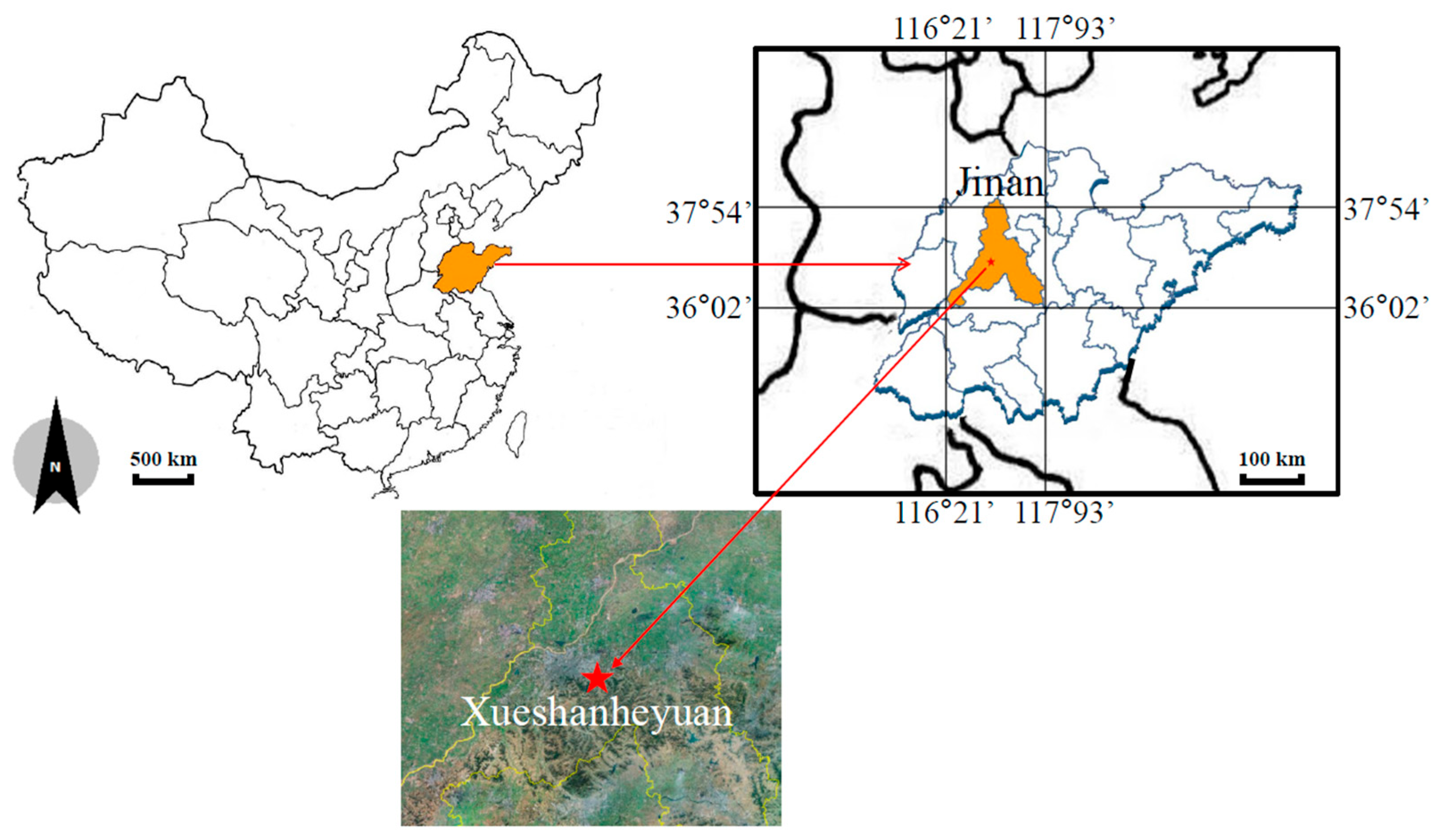
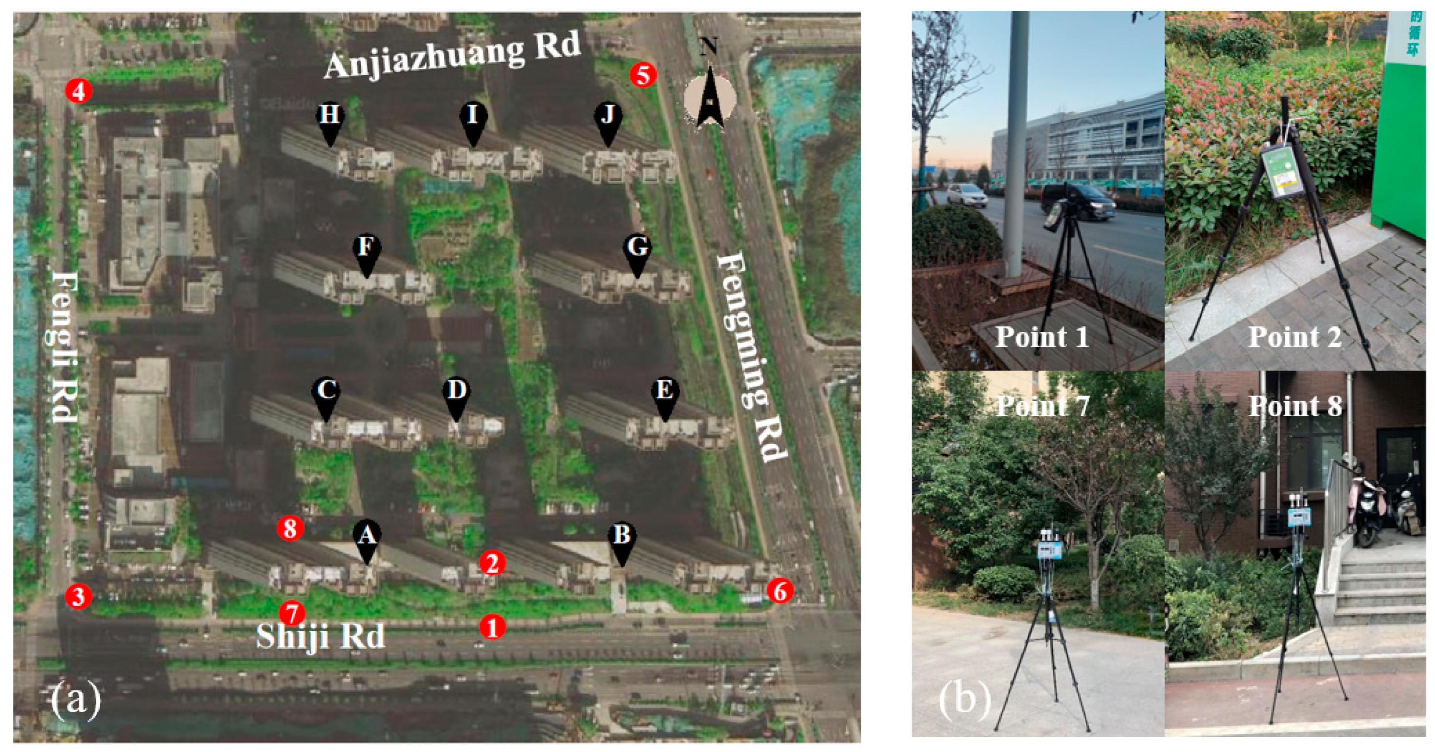
ENVI-met employs the following advection-diffusion equation to calculate the mass, momentum, energy budgets, and dispersion of gases and particles in the atmosphere:

$${\displaystyle \frac{\partial \chi }{\partial t}}+u{\displaystyle \frac{\partial \chi }{\partial x}}+v{\displaystyle \frac{\partial \chi }{\partial y}}+w{\displaystyle \frac{\partial \chi }{\partial z}}={\displaystyle \frac{\partial }{\partial x}}\left(K_x{\displaystyle \frac{\partial \chi }{\partial x}}\right)+{\displaystyle \frac{\partial }{\partial y}}\left(K_x{\displaystyle \frac{\partial \chi }{\partial y}}\right)+{\displaystyle \frac{\partial }{\partial z}}\left(K_x{\displaystyle \frac{\partial \chi }{\partial z}}\right)+Q_{\chi }\left(x,y,z\right)+S_{\chi }(x,y,z)$$

(11)

where χ represents the concentration of pollutants (mg/kg), Q_χ and S_χ represent the pollutant source coefficient and the deposition coefficient, respectively.

2.2. Site Details

Figure 2 shows the location and layout of the study area, which is Jinan, the capital of Shandong Province, located at 36°40′ north latitude and 117°00′ east longitude. Note that Jinan belongs to a cold region. According to meteorological data, it reaches the highest temperature in July with daily average values of 35 °C, while it reaches the lowest temperature in January with daily average values of −8 °C. In winter, the prevailing wind is from the north, with average speeds in the range of 1.5–2.2 m/s. In summer, the prevailing wind is from the southeast, with average speeds in the range of 1.8–2.6 m/s. Jinan is classified as a large city with a dense population and heavy traffic congestion, significantly affected by traffic-related pollutants.

In this study, a residential area, which consists of high-rise buildings (average height of almost 90 m) in Jinan is selected. It is densely arranged with a regular layout of buildings. It spans approximately 360 m in the east–west direction and 320 m in the north–south direction. Its main roads include Century Avenue to the south and Fengming Road to the east, with each having four lanes in each direction. The west and north sides have collector streets of single lanes in each direction. There are no industrial pollution sources near the residential area, which makes automobile exhausts the primary source of atmospheric particulate matter. Figure 3 shows photos of the study area and measuring points. Due to the variations in pollutants, outdoor thermal environment, and building layout, eight measurement points were established. Measurement point 1, within the green belt between the motorized lane and the pedestrian walkway, was selected, and point 2 was vertically placed between two buildings, 40 m apart. Points 3–6 were set at different azimuth angles within the neighborhood, to be used in the following outdoor environment analysis. Points 7 and 8 were placed on the windward and leeward sides of building A.

2.3. Field Measurements

To validate the accuracy of the model, field measurements were conducted during weekdays from 29 to 30 September and 27 to 28 October, with daily monitoring spanning from 7:00 to 19:00. The PM_2.5 concentrations were measured using MetOne 831 laser particle counters (Met One Instruments, Grants Pass, OR, USA). The MetOne sensor adopts the same satellite aerosol optical depth (AOD) measurement standard as the NASA MODIS system [33]; its accuracy has been validated by Hafkenscheid et al. [34]. To evaluate its performance, this study conducted synchronous comparative measurements at a height of 1.5 m using three PM_2.5 monitoring devices: the MetOne 831 laser particle counter, CEM DT-9883 air-quality detector (Shenzhen Everbest Machinery Industry Co., Ltd., Shenzhen, China), and Handheld 3016 IAQ monitor (Lighthouse Worldwide Solutions, Grants Pass, OR, USA). The results demonstrated strong consistency (R² > 0.85) in PM_2.5 concentration measurements among the three instruments. The air temperature and relative humidity (RH) were recorded using a JA-IAQ-50 multifunctional tester (Beijing Shijijiantong Technology Co., Beijing, China), with the measurement height fixed at 1.5 m (the height of human respiration) [35,36]. The details of the equipment are listed in

Table 1. The measurement parameters and devices used for monitoring.

Instrument	Parameters	Accuracy	Measuring Range
MetOne 831 laser particle counters	PM2.5	0.1 μg/m3	0–1000 μg/m3
JA-IAQ-50 multifunctional tester	Ta	0.5 °C	−22–125 °C
JA-IAQ-50 multifunctional tester	RH	3%	0–3%

. The hourly traffic flow was recorded by capturing videos at different time intervals on the road. The compiled traffic volume data, classified into three distinct vehicle categories—passenger cars (PC), buses (BUS), and light-duty vehicles (LDV)—are comprehensively presented in

Table 2. Hourly traffic value: vehicle type-specific volume statistics.

Hour	PC (Veh/h)	LDV (Veh/h)	Bus (Veh/h)	Total (Veh/h)
6–7	860	50	48	958
7–8	989	52	75	1116
8–9	1002	58	70	1130
9–10	865	56	68	989
10–11	820	53	55	928
11–12	825	54	58	937
12–13	886	53	54	993
13–14	921	56	53	1030
14–15	844	54	50	948
15–16	864	55	53	972
16–17	978	58	63	1099
17–18	1167	58	70	1295
18–19	1032	48	65	1145
19–20	760	45	50	855

. Relevant road parameters were determined using online Baidu satellite images [37].

2.4. Simulation

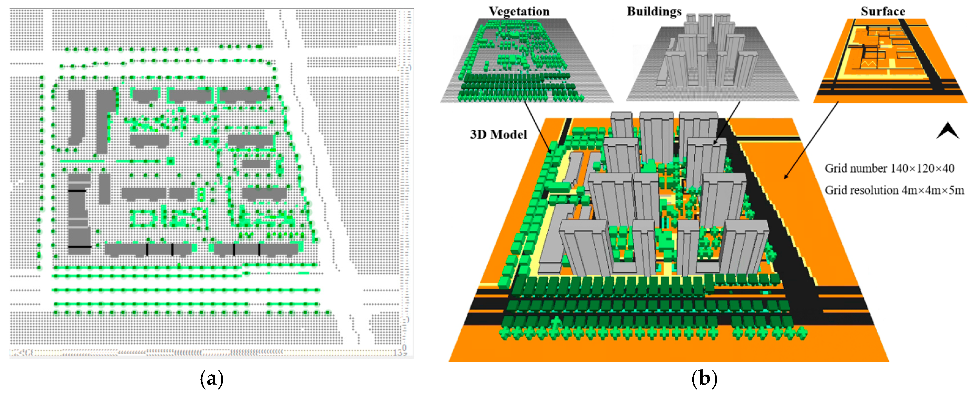
2.4.1. Model Configuration

The input parameters for ENVI-met 5.1 are divided into input files and configuration files. The input files describe the physical attributes of the study area, including the buildings, vegetation, and the surface, all set according to actual conditions, as shown in Figure 4. To ensure the reliability of the simulation results and effectively mitigate boundary effects, 10–20 grid cells were reserved between the buildings and the model boundaries; in the vertical direction, a space of one building height was reserved. Based on these parameter settings, the final three-dimensional model was constructed with a spatial scale of 560 m× 480 m × 200 m; the grid configuration was set to 140 × 120 × 40 computational units. The configuration files involve the parameter settings for model simulation, including grid settings, simulation date, start time, duration, meteorological parameters, and pollutant settings. Due to the location of the main traffic artery to the south of the community, testing was conducted during weather conditions with a dominant south wind. Additionally, since the software does not accurately simulate instantaneous cloud conditions, clear days with no clouds were selected for measurement. Ultimately, 30 September and 28 October were determined as sampling days. The duration of the model was set for 24 h, with the first 12 h designated for initialization and the following 12 h for valid data collection. To obtain daytime data for the two sampling days, the start times were set for 19:00 on 29 September and 19:00 on 27 October, respectively. The meteorological parameters consist of temperature, humidity, solar radiation, and wind speed. Using fully enforced meteorological boundary conditions, calibration and verification were performed with actual measurement data. The test data were imported into the ForcingManager function in CSV file format to create the enforced meteorological conditions for 29–30 September and 27–28 October. The T_a and RH were enforced accordingly. Since the measurement days were clear and cloudless, the cloud cover value was set to 0. The wind speed was set to the average value of 2 m/s for the measurement days, with the wind direction corresponding to the dominant wind direction at the time (south). For the optimized conditions, typical meteorological year data were used; the EPW format file was similarly imported into the ForcingManager function. The finalized parameter configuration for the ENVI-met 5.1 model is shown in

Table 3. ENVI-met model parameter configuration.

Variable	Value
Simulation Days	29 September 19:00 p.m.	27 October 19:00 p.m.
Coordination	117°17′ E, 36°69′ N	117°17′ E, 36°69′ N
Simultion duration (h)	24	24
Output interval of the data (h)	1	1
Domain cells	140 × 120 × 40	140 × 120 × 40
Spatial resolution	4 m × 4 m × 5 m	4 m × 4 m × 5 m
Tree (m)	Height = 10, Wide = 7	Height = 10, Wide = 7
Hedge (m)	Height = 1.5	Height = 1.5
Grass	Height = 0.25	Height = 0.25
Temperature (°C)	Min = 19.8, Max = 31.5	Min = 12.5, Max = 22.9
Humidity (%)	Min = 60, Max = 100	Min = 30, Max = 90
Wind speed at 10 m (m/s)	2	2
Cloud cover	0	0
Wind direction (°)	180 (South)	180 (South)
Surface albedo	Walls 0.2; Roofs 0.2 and 0.3	Walls 0.2; Roofs 0.2 and 0.3
Daily traffic value (Veh/24 h)	15,000	15,000
Linear source emission rate (μg/s/m)	12.7	12.7
Pollutant height (m)	0.3	0.3
Background concentration (μg/m3)	60	60

.

2.4.2. Model Calibration and Validation

The selection of grid size in the model involves a trade-off: excessively large grid settings can impact the accuracy of the model, while excessively small grid settings lead to longer simulation times and higher computer configuration requirements. Therefore, after comprehensive consideration, three grid sizes were established: 2 m × 2 m × 2 m; 4 m × 4 m × 5 m; and 6 m × 6 m × 8 m. Each grid size was simulated once on both sampling days. The model’s accuracy was objectively evaluated using multiple statistical metrics: the coefficient of determination (R²); root mean square error (RMSE); mean absolute error (MAE); mean bias (MB); and mean fractional bias (MFB). R² evaluates the goodness between measured and simulated values. It is in the range of 0–1, while values closer to 1 indicate a better fit. The RMSE is commonly used to evaluate the degree to which the ENVI-met 5.1 simulation results are different from the actual values. Note that a smaller value indicates a higher performance. MAE directly quantifies the mean of prediction errors, with smaller values being preferable. MB indicates the direction of systematic bias in predicted values—positive values suggest a general overestimation by the model, while negative values indicate underestimation. MFB is a standardized measure of systematic bias, with values closer to 0 indicating smaller deviations. Validation focused on key meteorological parameters (T_a, RH) and PM_2.5 concentrations, with all statistical metrics computed for paired observed and simulated values.

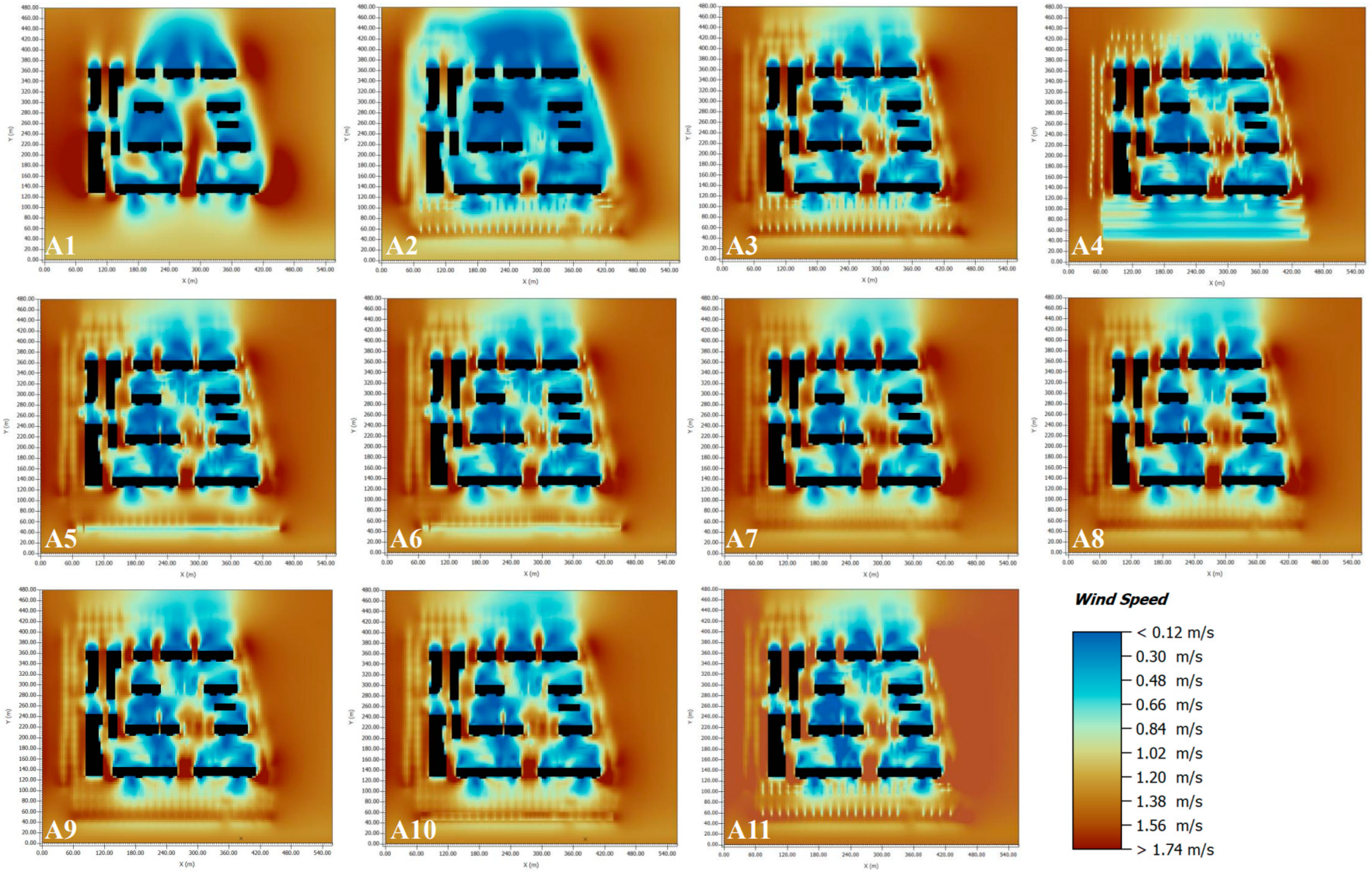
2.4.3. Vegetation Layout

This paper aims to study the impacts of different vegetation parameters (i.e., the tree crown shape, vegetation type, spacing between street trees, and LAD) on the outdoor environment. The tree crown shapes were set as spherical and cylindric based on common tree species in Jinan City, corresponding to cases A2 and A3 in

Table 4. The various cases considered in this study.

Cases	Crown Shape	Type	Tree Spacing (m)	LAD
A1	–	–	–	–
A2	Spherical	Trees and shrubs	8	2
A3	Cylindric	Trees and shrubs	8	2
A4	Cylindric	Shrubs	4	2
A5	Cylindric	Trees	4	2
A6	Cylindric	Tall trees on the inner row	8	2
A7	Cylindric	Tall trees on the outer row	8	2
A8	Cylindric	Trees	8	2
A9	Cylindric	Trees and shrubs	8	0.5
A10	Cylindric	Trees and shrubs	8	1.0
A11	Cylindric	Trees and shrubs	8	1.5

, respectively. The vegetation types included shrubs (A4), trees (A5), and a combination of trees and shrubs which was further divided into three cases: alternate planting of trees and shrubs (A3); inner rows of trees and outer rows of shrubs (A6); and inner rows of shrubs and outer rows of trees (A7). The spacing between the street trees was set to 4 m and 8 m, corresponding to A5 and A8 in Table 4, respectively. The LAD values for vegetation were set to 0.5, 1, 1.5, and 2, corresponding to cases A9, A10, A11, and A3, respectively. These vegetation configurations were designed in two different orientations with respect to the prevailing wind. The south and east sides of the neighborhood are both congested main roads. Therefore, the model included vertical and horizontal orientations with respect to the wind direction.

2.5. Evaluation Indices

In this paper, the percentage reduction method and the (Physiological Equivalent Temperature star) PET* index are used to evaluate the outdoor air quality and thermal environment, respectively. The reduction efficiency is calculated as:

$$P={\displaystyle \frac{(C_s-C_m)}{C_m}}\times 100\%$$

(12)

where C_s is the PM_2.5 concentration value at the roadside (μg/m³) and C_m is the concentration value at various distances from the street (μg/m³).

PET* is an improved index derived from the traditional Physiological Equivalent Temperature (PET), commonly used to evaluate outdoor thermal environments [38,39]. Similar to PET, It is defined as the temperature of a given environment at which the core and skin temperatures of a person match those in a standard setting (i.e., T_a of 20 °C, RH of 50%, and air velocity of 0.1 m/s) [40]. The PET* model differs from the conventional PET by redesigning the energy balance equation of the skin node and expanding output variables [38,39].

3. Results

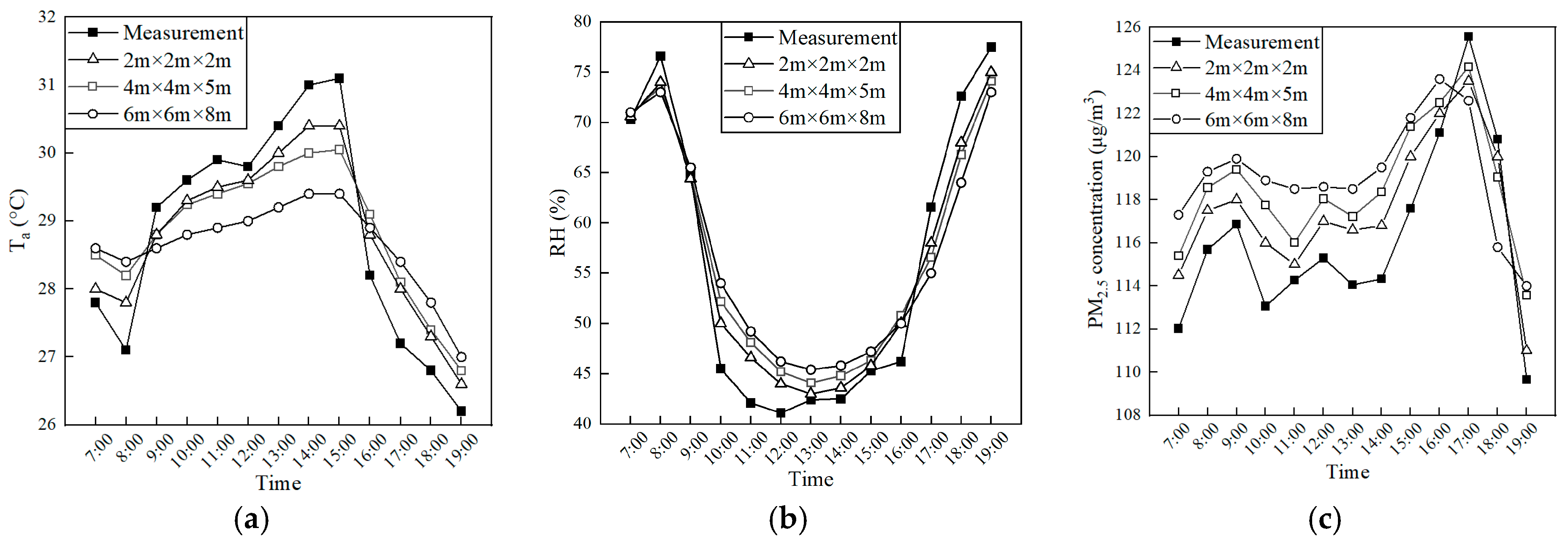
3.1. Comparison of Measured and Simulated Values

Figure 5 shows the T_a, RH, and PM_2.5 under three grid conditions. The used meteorological data were from 30 September, while the PM_2.5 data were from 28 October. The figure indicates that under all three grid conditions, the trend of the measured values for T_a, RH, and PM_2.5 is consistent with the simulated values. The simulation results with a grid size of 2 m × 2 m × 2 m are closer to the measured values, while the results with a grid size of 6 m × 6 m × 8 m differ significantly from the measured values.

Table 5. Mesh sensitivity: mean absolute errors of T_a, RH, and PM_2.5 between experimentally measured values and simulated values for different cell sizes.

Cell Size	Ta	RH	PM2.5
2 m × 2 m × 2 m	0.18%	0.59%	0.21%
4 m × 4 m × 5 m	0.24%	1.12%	0.68%
6 m × 6 m × 8 m	0.46%	8.16%	7.90%

presents the average percentage variations between the experimental measurements and simulated values of T_a, RH, and PM_2.5 for different grid sizes. It was observed that increasing the grid size has a minor impact on T_a, but a significant impact on RH and PM_2.5, especially under the 6 m × 6 m × 8 m condition, where the percentage changes reached 8.16% and 7.9%, respectively. Although the 2 m × 2 m × 2 m size is closer to the true values, it was not adopted due to the lengthy simulation time.

Since ENVI-met 5.1 cannot simulate changes in wind speed over time, only the contour of the wind speed was presented for validation. Figure 6 illustrates the distribution of wind speed within the study area. The wind speed in the surrounding environment is approximately 2 m/s, which is not far from the set value. On the streets near the residential area, the wind speed ranges from 1 m/s to 1.5 m/s, while the wind speed inside the residential area is less than 1 m/s. This result aligns with the actual conditions of the study area.

Table 6. Results of the measurement point obtained by the proposed model based on the T_a, RH, and PM_2.5 concentrations.

	Ta	RH	PM2.5
R2	0.96	0.91	0.89
RMSE	0.76	2.06	1.88
MAE	0.63	1.83	1.69
MB	−0.18	0.67	1.26
MFB	−0.07	0.13	0.21

presents the R², RMSE, MAE, MB and MFB between the numerical simulation results and experimental measurements under a grid size of 4 m × 4 m × 5 m.

Table 7. Experimental validation results from other references.

Reference	City	Variable	R2	RMSE	MAE	MB
[41]	Nanjing, China	Ta	–	1.08	–	0.7
		RH	–	7.9	–	4.2
[42]	Guangzhou, China	Ta	0.9821–0.9837	1.0176–1.0762	0.9578–0.9597	–
		RH	0.9801–0.9821	0.9598–1.1704	0.7681–0.8086	–
[43]	Guangzhou, China	PM2.5	0.977	–	–	–
[44]	Guangzhou and Dongguan, China	Ta	0.89	1.21	–	1.05
		RH	0.80	1.51	–	1.33
[45]	Tel Aviv-Yafo, Israel	Ta	–	0.85–1.08	0.65–0.89	−0.03/0.53
		RH	–	3.84–4.04	3.78–3.96	3.78–3.96
[46]	Phoenix, USA	Ta	0.83–0.96	1.51–4.5	–	0.63–3.5
[47]	Bangkok, Thailand	PM2.5	0.77	0.495	–	–
[48]	Guangzhou, China	PM2.5	0.61–0.74	–	–	0.078–0.518
[49]	Bangkok, Thailand	Ta	0.763–0.975	1.194–1.679	–	–
		RH	0.788–0.979	2.106–4.844	–	–
[50]	Hong Kong, China	Ta	0.49–0.93	0.44–1.86	0.34–1.56	−1.54–(−0.13)/0.04–0.79
		RH	0.11–0.87	3.84–8.79	3.17–8.17	−8.09–(−0.73)
[51]	Melbourne, Australia	Ta	–	0.95–4.9	–	–
		RH	–	0.95–4.9	–	–
[52]	Bilbao, Spain	Ta	0.92–0.99	1.0–2.07	0.83–1.82	−1.54–(−0.17)

presents the validation results of models from other studies. The validation results demonstrate that the ENVI-met model achieved excellent performance in simulating air temperature (T_a); the R² is 0.96, which is 0.05 units higher than the average value from other studies. The model showed low error magnitudes (RMSE = 0.76, MAE = 0.63, MFB = −0.07), which were lower than most values presented in Table 7, with only slight underestimation (MB = −0.18). For relative humidity, the simulations maintained strong consistency (R² = 0.91, RMSE = 2.06, MAE = 1.83, MFB = 0.13) despite minor overestimation (MB = 0.67). Regarding PM_2.5, although the R² (0.89) was slightly lower than those for T_a and RH, it remained within the acceptable range (>0.8). RMSE (1.88), MAE (1.69), and MFB (0.21) fell within ideal levels, while the MB (1.26) indicated systematic overestimation of PM_2.5 concentrations by the model. All simulated errors fell within acceptable ranges, demonstrating the reliable performance of the ENVI-met model.

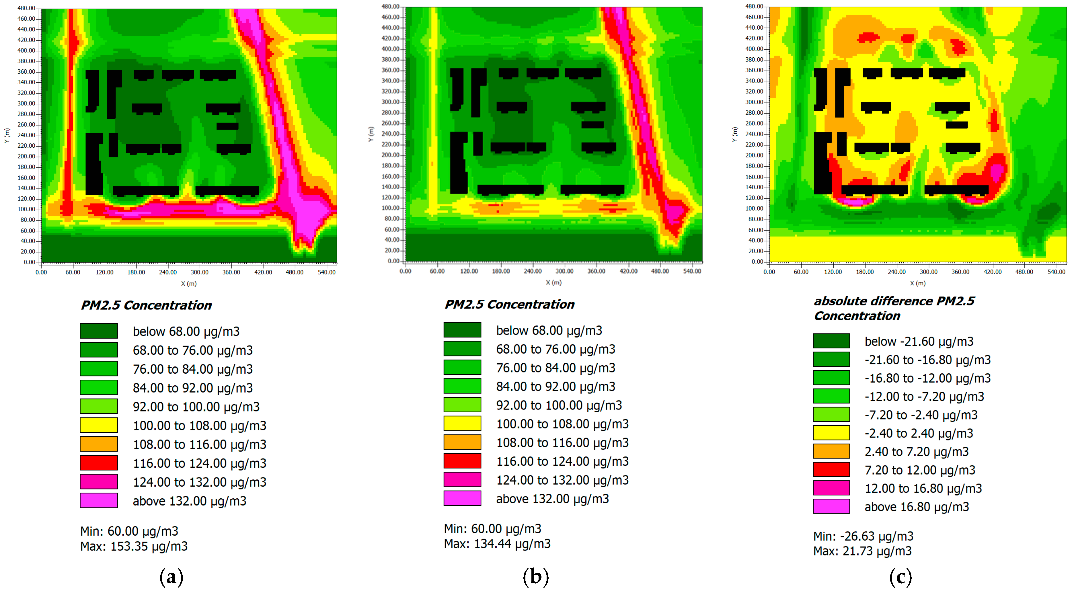
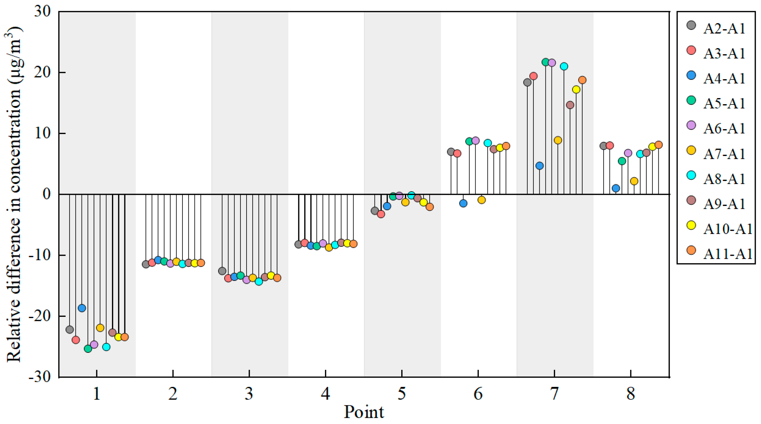
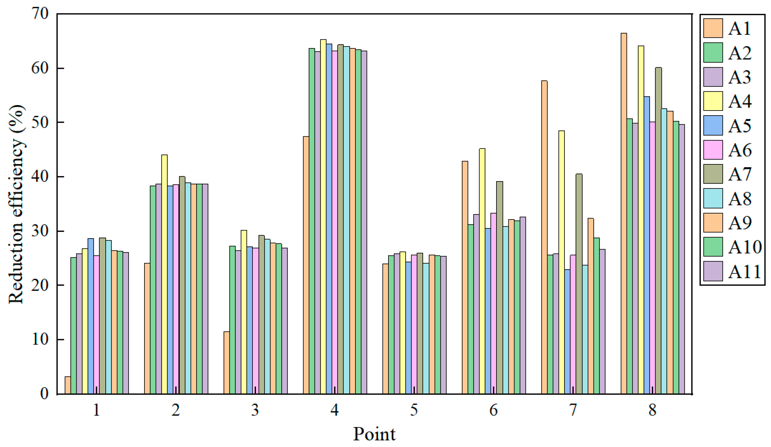
3.2. Impacts of Different Vegetation Configurations on the Air Quality

Figure 7 shows the distribution and differences in PM_2.5 concentrations between scenarios with and without vegetation. More precisely, Figure 7a illustrates the case without vegetation (A1) and with the highest PM_2.5 concentration reaching 153.35 μg/m³. Figure 7b displays the PM_2.5 concentration distribution under the typical vegetation configuration (A3), showing significantly lower concentrations compared to the non-vegetated case. The concentration changes are shown in Figure 7c, which presents the differences in PM_2.5 concentrations between scenarios with (A3) and without (A1) vegetation. The green areas denote a decrease in PM_2.5 concentrations due to the addition of vegetation, which indicates an improved air quality. The orange and red areas denote worsened air quality after adding vegetation, while the yellow areas indicate minimal impact of vegetation on pollutant levels. It can be seen that when the vegetation increases, the pollutant concentrations on roads and sidewalks significantly decrease and reach 26.63 μg/m³, which demonstrates that the adsorption role of the vegetation helps the pollutant deposition. However, the concentration of pollutants in the residential area, especially around buildings, with an increment in the range of 2.5–17.5 μg/m³, may be due to the impact of the buildings on the wind environment, which limits the pollutant dispersion. Therefore, adding vegetation may have positive or negative impacts on the air quality. Consequently, accurate choices, based on specific locations, are crucial. In addition, it can be observed that pollutants from the main road on the southern side have a greater impact within the residential area due to prevailing summer winds. Moreover, traffic pollutants on the east and west sides have a minor impact within the residential area. This emphasizes the need for studying the impact of streets perpendicular to the prevailing wind direction on pollutants within residential areas.

Based on the wind speed distribution map (Figure 8), it can be observed that increasing vegetation can reduce wind speed. In street environments, the wind speed distribution, at a height of 1.5 m, is significantly influenced by the structural characteristics of different types of vegetation. Studies have shown that tree trunks, canopies, and branches alter the airflow structure within street canyons [18]. When wind flows through a street canyon, trees force the airflow to disperse and bypass them, potentially generating localized turbulence. This increases the turbulence intensity within the street canyon, which aids in the dispersion of PM_2.5. In contrast, shrubs significantly obstruct airflow due to their dense foliage, substantially reducing local wind speed. The turbulence induced by shrubs can also promote vertical air mixing, thereby partially mitigating pollutant accumulation. Grass has a minimal impact on wind speed at 1.5 m. Overall, under the influence of trees and shrubs, the concentrations of PM_2.5 on streets generally decrease. However, around buildings, the shielding effect of buildings reduces wind speed on the leeward side. Under low wind speed conditions, pollutants struggle to disperse, leading to localized accumulation and an increase in PM_2.5 concentrations.

Figure 9 shows the differences in PM_2.5 concentrations at eight measurement points under various greening conditions compared to the condition without vegetation, where the positive and negative values denote increase and decrease in pollutant concentrations after the addition of vegetation, respectively. In general, the PM_2.5 concentrations at measurement points 1–3 are decreased by more than 10 μg/m³. This is due to the fact that these measurement points are located on the southern side of the building, where there is ample sunlight and good ventilation, which facilitates the diffusion of pollutants. Measurement point 5 shows a slight decrease in PM_2.5 concentrations within the range of 0.21–3.2 μg/m³, which is due to its distance from the main road, indicating minimal impact of the added vegetation. Measurement points 6–8 exhibit an increase in PM_2.5 concentrations due to the impact of buildings and wind direction. Measurement point 7 reaches 21.75 μg/m³, intensifying the environmental pollution from PM_2.5. A detailed analysis of individual measurement points shows no significant differences between, A2, A3, and the case without vegetation, which indicates that the shape of the canopy has minimal impact on PM_2.5. By comparing the A3, A4, A5, A6, and A7 cases, it can be deduced that significant variations in pollutant concentrations exist in the region where the PM_2.5 concentrations decrease. More precisely, measurement point 1 shows the most significant change (A5 > A6 > A3 > A7 > A4), while measurement points 2–5 exhibit similar differences across all the cases. In the region where the PM_2.5 concentrations increase, the pollutant elevation under A4 is much lower compared with the other cases. In particular, at the prominent measurement point 7, the increase in the PM_2.5 concentrations under other cases is in the range of 19.46–21.75 μg/m³, while in the A4 case, the increase is only 4.73 μg/m³. Thus, planting shrubs alone is the most beneficial for outdoor air-quality improvement. A comparison between A6 and A7 shows that planting shrubs on the inner part leads to better air-quality improvement compared with planting trees. The PM_2.5 concentrations for A7 are 0.3–12.7 μg/m³ lower than that for A6. No significant differences are observed between A5 and A8, which indicates that the row spacing of trees has a slight impact on PM_2.5. By comparing the differences between A9, A10, A11, A3, and A1, it can be deduced that, when the LAD increases, the increase in pollutants is greater, while the decrease is not significant. This demonstrates that the increase in LAD of the vegetation intensifies the environmental pollution.

The reduction efficiency of PM_2.5 at various monitoring points was calculated using Equation (12), while the edge of the motor lane was set to 0 m, as shown in Figure 10. In cases with vegetation, the attenuation rates of PM_2.5 at monitoring points 1–4 are higher than A1; monitoring point 1 exhibits the most significant improvement. The latter, located closest to the motor lane, has an attenuation rate of only 3.27% without vegetation. After adding vegetation, its attenuation rate is increased to 25.12–28.85%, which indicates an improvement in outdoor air quality due to greening. For monitoring points 6–8, the PM_2.5 attenuation rates after greening are lower than those in the non-greening case (A1), which indicates increased pollution levels after greening. Among all the monitoring points, A4 exhibits the highest attenuation rates, reaching 65.34% and 64.19% at monitoring points 4 and 8, respectively. The vegetation in A4, consisting of shrubs, facilitates the diffusion of pollutants upwards. It can be observed that the shape of the canopies and the spacing between the trees slightly affect the PM_2.5 concentrations. By comparing cases A9, A10, A11, and A3, it can be deduced that, when the vegetation LAD increases, the attenuation rates of PM_2.5 gradually and slightly decrease, which is consistent with the previous results.

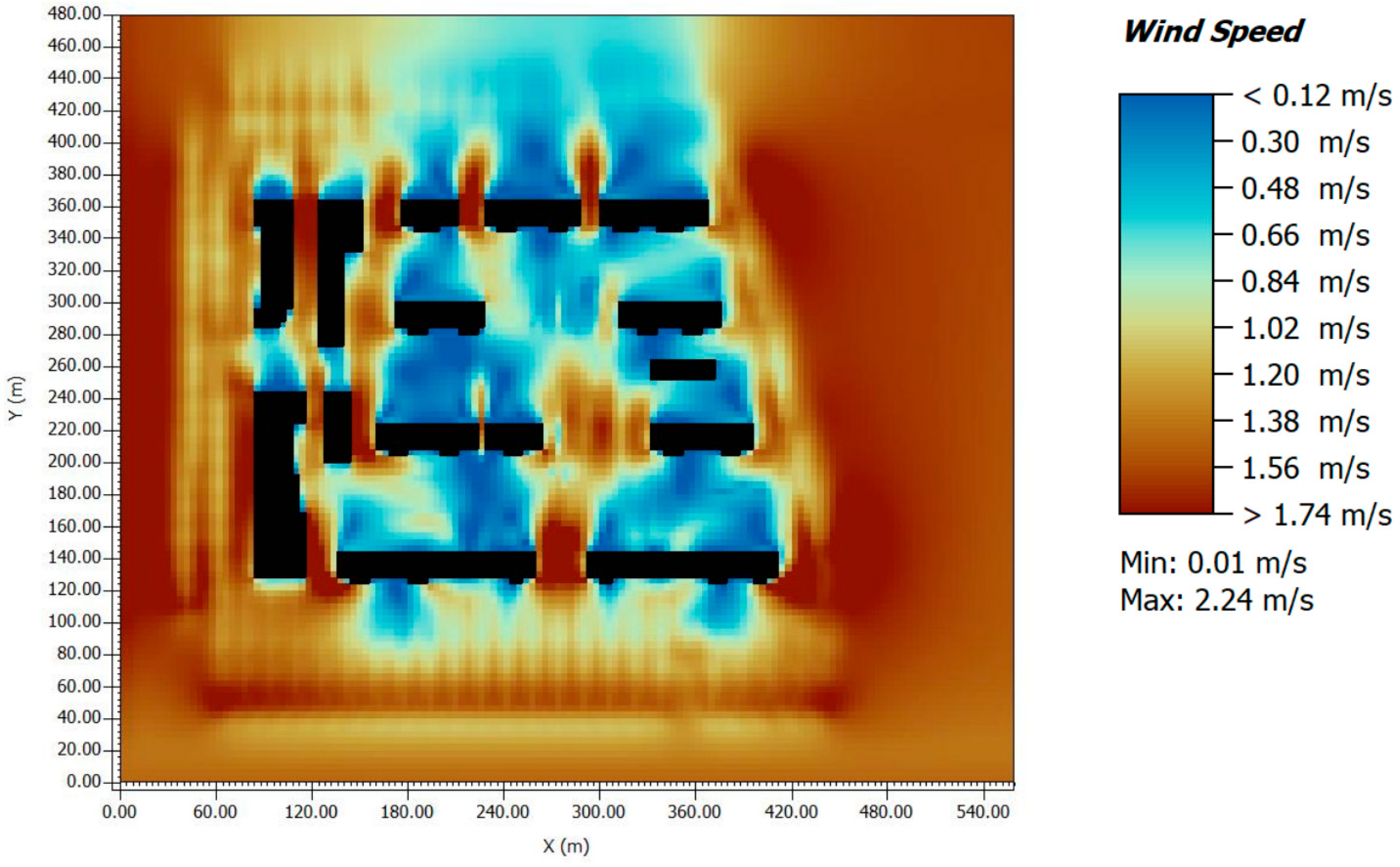
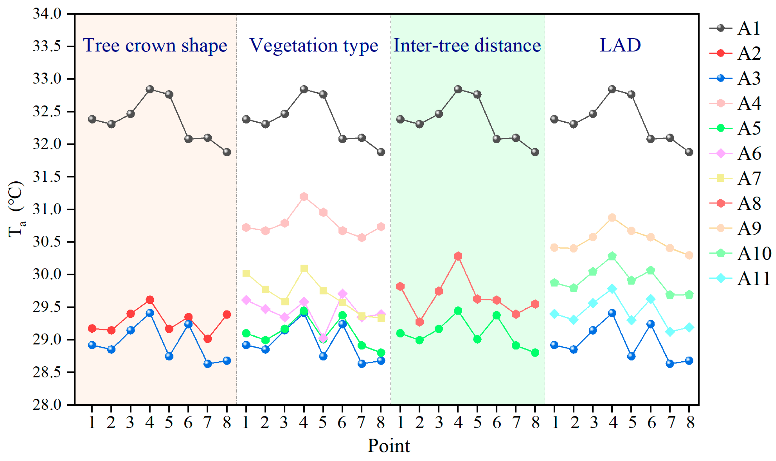
3.3. Impacts of Different Vegetation Configurations on the Outdoor Thermal Environment

In the study of the outdoor thermal environment, the differences in meteorological parameters (T_a) and human thermal comfort index (PET*) between different vegetation configurations were analyzed. Figure 11 compares the horizontal distributions of T_a and PET* at pedestrian height (1.5 m) between the typical vegetation configuration case A3 and without vegetation A1 at 14:00. It can be seen that both T_a and PET* decrease, which demonstrates that the increase in vegetation improves the outdoor thermal environment. A comparison with the vegetation layout in Figure 4 shows a significant improvement in the thermal environment in the vegetation-covered area. The T_a and PET* are, respectively, decreased by 3–4.8 °C and 8–12.8 °C, while the other areas experience a cooling effect of less than 3 °C and PET* values decreased by less than 8 °C. Due to the impact of the southern wind, the temperature drop on the north side of the area is higher than that on the south side. Moreover, it can be seen that the PET* values are the least affected by the wind direction.

Figure 12 shows the temperatures at different measuring points for various cases. It employs differentially colored rectangular boxes to represent respective variables, thereby demonstrating the characteristic effects of vegetation configuration on air temperature. It can be seen that after greening, the temperatures at all the points decrease. In particular, A4 has the least significant cooling effect, with an average temperature decrease of 1.7 °C, which may be due to the presence of low shrubs leading to higher solar radiation and thus a poorer cooling effect. Compared with A2, the cooling effect of A3 is better, which indicates the outperformance of a cylindric tree canopy in reducing summer temperatures. By comparing A3, A4, A5, A6, and A7, it can be deduced that A3 has the best cooling effect, followed by A5, A6, and A7, while A4 has the least improvement. This demonstrates that a combination of trees and shrubs is more effective in reducing temperatures than having only trees or shrubs. In addition, the impact of trees at the inner or outer row on the temperature is minimal. A5 and A8, respectively, have average temperature decreases of 3.67 °C and 3.18 °C, which demonstrates that the reduction in the distance between trees improves the T_a. Furthermore, a comparison between A9, A10, A11, and A3 shows that, when the LAD increases, the cooling effects significantly increase, which is the opposite of the trend of change in the PM_2.5 concentrations.

Figure 13 shows the PET* values across measurement points for different scenarios. It can be seen that the increase in greenery contributes to the PET* reduction, which enhances the outdoor thermal environment. In scenarios without greenery (A1), the PET* at measurement point 4 reaches 44.5 °C. Existing studies [53,54] have shown that in cold regions, a PET* exceeding 40 °C can make outdoor personnel feel extremely hot, which significantly affects health. Figure 13 reveals that the canopy shape (cylindrical or spherical) has a negligible influence on PET*, whereas vegetation type (shrubs or trees) plays a major role. Scenario A4 (all shrubs) has the highest PET* (>40 °C), yet still reduces PET* by 3.17 °C. Tall trees, however, provide greater cooling, lowering PET* by up to 9.68 °C. Furthermore, closer tree spacing and higher LAD further enhance thermal comfort, consistent with temperature trends. Spatially, street-proximal areas (Points 1 and 7) exhibit the most substantial thermal mitigation (ΔPET* up to 10.9 °C), primarily due to direct canopy shading and evapotranspiration. In contrast, the downwind building zone (Point 8) shows minimal improvement (ΔPET* = 3.46 °C).

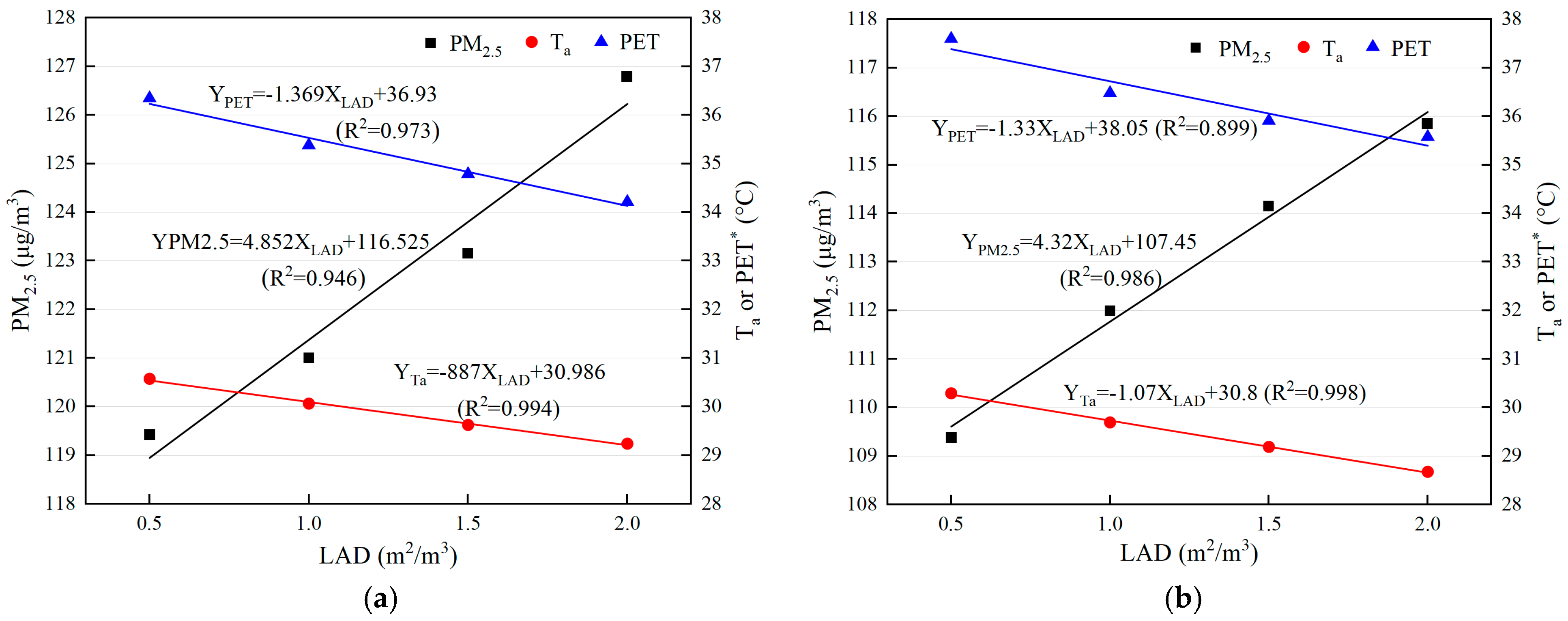
3.4. Impact of the Greening Configuration on the Outdoor Environment

Existing studies have shown that an increase in greening improved the outdoor thermal environment in summer [24,55]. However, it has a dual impact on the air quality. More precisely, the pollutant concentrations are reduced on streets with vegetation cover, while they tend to increase in residential areas, especially around apartment buildings. It has been shown that the greatest contradiction lies in the impact of the vegetation LAD on the outdoor thermal environment and air quality. Therefore, this study focuses on point 6, which has the highest PM_2.5 concentrations and is also the most affected point by the LAD. The impacts of the LAD (A3, A9, A10, and A11) on the outdoor environment are illustrated in Figure 14a. According to the results presented in Section 3.2, the negative impact of the vegetation on the environment is more significant around buildings, especially on the side adjacent to Shiji Road. As a result, the relationships between the LAD and PM_2.5, T_a, and PET* at intervals of 15 m are recorded. The obtained results are illustrated in Figure 14b.

Near the main road, an LAD increase negatively affects the reduction in pollutant concentrations while facilitating a decrease in summer T_a and PET*. According to the fitted model presented in point 6, an LAD increase of 1 m²/m results in a PM_2.5 concentration increase of 4.852 μg/m³, while T_a and PET* decrease of 0.887 °C and 1.369 °C, respectively. In general, in the area on the south side of the residential community near the main traffic artery, the impact of the LAD on T_a and PET* is more significant, with reductions of 1.07 °C and 1.93 °C, respectively. The impact of the LAD on PM_2.5 concentrations is lower. That is, for an LAD increase of 1 m²/m³, the PM_2.5 concentrations increase by 4.32 μg/m³. A conducted analysis shows that, in residential areas adjacent to major traffic roads, enhancing outdoor environments through increased vegetation can result in increasing PM_2.5 concentrations. In particular, for every 1 °C decrease in outdoor temperature, the PM_2.5 concentrations will increase by 4.04 μg/m³; for every 1 °C decrease in PET*, it will increase by 2.24 μg/m³.

4. Discussion

4.1. Vegetation Configuration and Environmental Trade-Offs

This study evaluated greening strategies in a high-rise residential community using ENVI-met 5.1 simulations. Our key innovation lies in quantifying the precise relationship between LAD and its dual effects: while each 1 m²/m³ increase in LAD reduces T_a by 1.07 °C and PET* by 1.93 °C, it simultaneously elevates PM_2.5 concentrations by 4.32 μg/m³ under low-wind conditions. While this aligns with prior findings on vegetation-induced microclimate improvements [56], our study reveals a key nuance—strategic shrub placement (inner rows) reduces roadside PM_2.5 by 26.63 μg/m³ without compromising thermal comfort.

Based on these findings, we identify optimal vegetation configurations for balancing outdoor air quality and thermal performance. Shrubs outperform trees in reducing PM_2.5 (Section 3.2), while a tree–shrub combination achieves the best thermal improvement (Section 3.3). Further analysis shows that planting shrubs on inner rows and trees on outer rows (A7) lowers PM_2.5 by 0.3–12.7 μg/m³ compared to the reverse arrangement (A6), with minimal impact on thermal conditions. Thus, the shrub-inner/tree-outer configuration emerges as the most advantageous strategy.

4.2. Urban Ventilation: Mitigating Heat Islands and Pollution

This study underscores the dual function of urban ventilation systems in mitigating heat island effects while regulating pollutant dispersion. Although dense vegetation provides cooling benefits, it may simultaneously restrict airflow and promote PM_2.5 accumulation under stagnant atmospheric conditions. While trees reduce street-level PM_2.5 concentrations by 26.63 µg/m³ through canopy adsorption and trunk-induced turbulence (at 1.5 m height), their aerodynamic resistance simultaneously increases building leeward-side PM2.5 levels by 17.5 µg/m³—a spatial trade-off that has been overlooked in previous studies [57]. Liu et al. [58] demonstrated that the influence of different vegetation types planted at various street locations on traffic pollutants exhibits significant variation. A comparative analysis of similar studies across diverse climatic regions [4,25] further reveals that optimal urban greening strategies must carefully balance vegetation with aerodynamic permeability to ensure effective ventilation. Zhang et al. [59] demonstrated this phenomenon in their investigation of urban morphology’s effects on thermal environment and pollutant dispersion patterns.

4.3. Limitations and Future Directions

Indoor–Outdoor Pollution Disparities: while we focused on outdoor PM_2.5, future work should integrate indoor–outdoor coupling, as 80% of indoor PM_2.5 originates outdoors [60].

Case Specificity: Our findings are based on Jinan’s high-rise residential typology under specific meteorological conditions. Further research should validate these findings across diverse urban settings and scales to enhance the adaptability of greening configurations.

Pollutant Scope: We prioritized aerodynamic effects but omitted biophilic design synergies. Future studies could combine vegetation with porous materials or green walls to enhance both thermal and air-quality benefits.

5. Conclusions

The research investigated the impact of four factors—plant types, canopy shapes, spacing of street trees, and LAD—on the outdoor thermal environment and PM_2.5 concentrations through ten different greening scenarios, leading to the following conclusions:

In residential areas near major roads, traffic-derived PM_2.5 reached 141.94 µg/m³. Increasing the vegetation may have positive or negative impacts on the air quality. Vegetation cover on urban main roads and sidewalks can improve the air quality and may reduce PM_2.5 concentrations by up to 26.63 μg/m³. On the contrary, air quality around buildings may decrease, which results in increasing PM_2.5 concentrations by up to 17.5 μg/m³.

The tree crown shape and spacing have minimal impacts on PM_2.5 concentrations. The vegetation type significantly affects PM_2.5 concentrations, while shrubs are more effective than trees in improving the air quality, achieving a PM_2.5 attenuation rate of up to 65.34%. In addition, planting shrubs on the inner row leads to better air-quality improvement than planting trees.

This study demonstrates that vegetation configuration significantly improves urban thermal comfort, with columnar-canopy trees at reduced spacing (A3) achieving optimal cooling performance (ΔT_a = 3–4.8 °C, ΔPET* = 8–12.8 °C). Dense tree planting (A5) improved thermal comfort (ΔPET* = 9.68 °C), while shrub-only arrangements (A4) showed limited effects (ΔT_a = 1.7 °C, ΔPET* = 3.17 °C).

As LAD increases, the outdoor thermal environment and air quality show opposing trends. In areas where vegetation raises PM_2.5 levels, a 1 m²/m³ LAD increase elevates PM_2.5 by 4.32 μg/m³, while T_a and PET* decrease by 1.07 °C and 1.93 °C, respectively. Thus, improving thermal conditions through vegetation reduces outdoor temperature by 1 °C at the cost of a 4.04 μg/m³ PM_2.5 increase, while a 1 °C PET* decrease raises PM_2.5 by 2.24 μg/m³.

For balanced air-quality and thermal benefits, plant shrubs on inner rows and trees on outer rows. Future studies should explore greening strategies in diverse urban contexts, particularly in rapidly developing cities.

References

1. Yola, L.; Adekunle, T.O.; Ayegbusi, O.G. The Impacts of Urban Configurations on Outdoor Thermal Perceptions: Case Studies of Flat Bandar Tasik Selatan and Surya Magna in Kuala Lumpur. Buildings 2022, 12, 1684. [Google Scholar] [CrossRef]
2. An, F.; Liu, J.; Lu, W.; Jareemit, D. Comparison of exposure to traffic-related pollutants on different commuting routes to a primary school in Jinan, China. Environ. Sci. Pollut. Res. 2022, 29, 43319–43340. [Google Scholar] [CrossRef]
3. Zhong, H.; Feng, J.; Lam, C.K.C.; Hang, J.; Hua, J.; Gu, Z. The impact of semi-open street roofs on urban pollutant exposure and pedestrian-level thermal comfort in 2-D street canyons. Build. Environ. 2023, 239, 110387. [Google Scholar] [CrossRef]
4. Fu, N.; Kim, M.K.; Huang, L.; Liu, J.; Chen, B.; Sharples, S. Investigating the reliability of estimating real-time air exchange rates in a building by using airborne particles, including PM1.0, PM2.5, and PM10: A case study in Suzhou, China. Atmos. Pollut. Res. 2024, 15, 101955. [Google Scholar] [CrossRef]
5. Rahman, M.; Meng, L. Examining the Spatial and Temporal Variation of PM2.5 and Its Linkage with Meteorological Conditions in Dhaka, Bangladesh. Atmosphere 2024, 15, 1426. [Google Scholar] [CrossRef]
6. Jia, X.; Zhang, B.; Yu, Y.; Xia, W.; Lu, Z.; Guo, X.; Xue, F. Greenness mitigate cause-specific mortality associated with air pollutants in ischemic and hemorrhagic stroke patients: An ecological health cohort study. Environ. Res. 2024, 251, 118512. [Google Scholar] [CrossRef]
7. An, F.; Liu, J.; Lu, W.; Jareemit, D. A review of the effect of traffic-related air pollution around schools on student health and its mitigation. J. Transp. Health 2021, 23, 101249. [Google Scholar] [CrossRef]
8. Ambient (Outdoor) Air Pollution. Available online: https://www.who.int/news-room/fact-sheets/detail/ambient-(outdoor)-air-quality-and-health (accessed on 2 August 2024).
9. Cheng, C.; Liu, Y.; Han, C.; Fang, Q.; Cui, F.; Li, X. Effects of extreme temperature events on deaths and its interaction with air pollution. Sci. Total Environ. 2024, 915, 170212. [Google Scholar] [CrossRef]
10. Kumar, P.; Sharma, A. Study on importance, procedure, and scope of outdoor thermal comfort—A review. Sustain. Cities Soc. 2020, 61, 102297. [Google Scholar] [CrossRef]
11. Qin, Y.; Sun, C.; Li, D.; Zhang, H.; Wang, H.; Duan, Y. Does urban air pollution have an impact on public health? Empirical evidence from 288 prefecture-level cities in China. Urban Clim. 2023, 51, 101660. [Google Scholar] [CrossRef]
12. Villani, M.G.; Russo, F.; Adani, M.; Piersanti, A.; Vitali, L.; Tinarelli, G.; Ciancarella, L.; Zanini, G.; Donateo, A.; Rinaldi, M.; et al. Evaluating the Impact of a Wall-Type Green Infrastructure on PM10 and NOx Concentrations in an Urban Street Environment. Atmosphere 2021, 12, 839. [Google Scholar] [CrossRef]
13. Kandelan, S.N.; Yeganeh, M.; Peyman, S.; Panchabikesan, K.; Eicker, U. Environmental study on greenery planning scenarios to improve the air quality in urban canyons. Sustain. Cities Soc. 2022, 83, 103993. [Google Scholar] [CrossRef]
14. Liu, C.; Dai, A.; Sheng, Q.; Zhu, Z. Study on the changes in concentration of air pollutants and influencing factors in road green spaces in Nanjing City during autumn and winter. Atmos. Pollut. Res. 2024, 15, 102003. [Google Scholar] [CrossRef]
15. Abdi, B.; Hami, A.; Zarehaghi, D. Impact of small-scale tree planting patterns on outdoor cooling and thermal comfort. Sustain. Cities Soc. 2020, 56, 102085. [Google Scholar] [CrossRef]
16. Tomson, M.; Kumar, P.; Barwise, Y.; Perez, P.; Forehead, H.; French, K.; Morawska, L.; Watts, J.F. Green infrastructure for air quality improvement in street canyons. Environ. Int. 2021, 146, 106288. [Google Scholar] [CrossRef]
17. Yang, L.; Liu, J.; Zhu, S. Evaluating the Effects of Different Improvement Strategies for the Outdoor Thermal Environment at a University Campus in the Summer: A Case Study in Northern China. Buildings 2022, 12, 2254. [Google Scholar] [CrossRef]
18. Abhijith, K.V.; Kumar, P.; Gallagher, J.; McNabola, A.; Baldauf, R.; Pilla, F.; Broderick, B.; Di Sabatino, S.; Pulvirenti, B. Air pollution abatement performances of green infrastructure in open road and built-up street canyon environments—A review. Atmos. Environ. 2017, 162, 71–86. [Google Scholar] [CrossRef]
19. Gromke, C.; Blocken, B. Influence of avenue-trees on air quality at the urban neighborhood scale. Part II: Traffic pollutant concentrations at pedestrian level. Environ. Pollut. 2015, 196, 176–184. [Google Scholar] [CrossRef]
20. Niza, I.L.; Bueno, A.M.; Gameiro da Silva, M.; Broday, E.E. Air quality and ventilation: Exploring solutions for healthy and sustainable urban environments in times of climate change. Results Eng. 2024, 24, 103157. [Google Scholar] [CrossRef]
21. Rafael, S.; Vicente, B.; Rodrigues, V.; Miranda, A.I.; Borrego, C.; Lopes, M. Impacts of green infrastructures on aerodynamic flow and air quality in Porto’s urban area. Atmos. Environ. 2018, 190, 317–330. [Google Scholar] [CrossRef]
22. Taleghani, M.; Clark, A.; Swan, W.; Mohegh, A. Air pollution in a microclimate; the impact of different green barriers on the dispersion. Sci. Total Environ. 2020, 711, 134649. [Google Scholar] [CrossRef] [PubMed]
23. Janhäll, S. Review on urban vegetation and particle air pollution—Deposition and dispersion. Atmos. Environ. 2015, 105, 130–137. [Google Scholar] [CrossRef]
24. Li, J.; Zhai, Z.; Ding, Y.; Li, H.; Deng, Y.; Chen, S.; Ye, L. Effect of optimal allocation of urban trees on the outdoor thermal environment in hot and humid areas: A case study of a university campus in Guangzhou, China. Energy Build. 2023, 300, 113640. [Google Scholar] [CrossRef]
25. Chen, X.; Pei, T.; Zhou, Z.; Teng, M.; He, L.; Luo, M.; Liu, X. Efficiency differences of roadside greenbelts with three configurations in removing coarse particles (PM10): A street scale investigation in Wuhan, China. Urban For. Urban Green. 2015, 14, 354–360. [Google Scholar] [CrossRef]
26. Maneechote, W.; Liu, J.; Jareemit, D. Cool Facades and Pavements: Mitigating Heat Stress and Improving Urban Thermal Conditions in Affordable Housing Project—A Case Study in Thailand. Future Cities Environ. 2024, 10, 1. [Google Scholar] [CrossRef]
27. Liu, Y.; Yang, X.; Liu, K.; Xu, R.; Pian, Y.; Liu, S. Mining of dynamic traffic-meteorology-atmospheric pollutant association rules based on Eclat method. Atmos. Pollut. Res. 2024, 15, 102305. [Google Scholar] [CrossRef]
28. Ren, L.; An, F.; Su, M.; Liu, J. Exposure Assessment of Traffic-Related Air Pollution Based on CFD and BP Neural Network and Artificial Intelligence Prediction of Optimal Route in an Urban Area. Buildings 2022, 12, 1227. [Google Scholar] [CrossRef]
29. Bruse, M.; Fleer, H. Simulating surface–plant–air interactions inside urban environments with a three dimensional numerical model. Environ. Model. Softw. 1998, 13, 373–384. [Google Scholar] [CrossRef]
30. Hofman, J.; Samson, R. Biomagnetic monitoring as a validation tool for local air quality models: A case study for an urban street canyon. Environ. Int. 2014, 70, 50–61. [Google Scholar] [CrossRef]
31. He, S.; Yang, L.; Liu, J.; Jareemit, D. Spatial distribution of PM2.5 concentration around high-rise residential buildings during peak traffic hours in autumn and winter seasons. Indoor Built Environ. 2024, 33, 757–778. [Google Scholar] [CrossRef]
32. Buccolieri, R.; Santiago, J.-L.; Rivas, E.; Sanchez, B. Review on urban tree modelling in CFD simulations: Aerodynamic, deposition and thermal effects. Indoor Built Environ. 2018, 31, 212–220. [Google Scholar] [CrossRef]
33. Malings, C.; Westervelt, D.M.; Hauryliuk, A.; Presto, A.A.; Grieshop, A.; Bittner, A.; Beekmann, M.; Subramanian, R. Application of low-cost fine particulate mass monitors to convert satellite aerosol optical depth to surface concentrations in North America and Africa. Atmos. Meas. Tech. 2020, 13, 3873–3892. [Google Scholar] [CrossRef]
34. Hafkenscheid, T.; Vonk, J. Evaluation of Equivalence of the MetOne BAM-1020 for the Measurement of PM2.5 in Ambient Air; National Institute for Public Health and the Environment: Bilthoven, The Netherlands, 2015. [Google Scholar]
35. Jia, S.; Wang, Y.; Wong, N.H.; Weng, Q. A hybrid framework for assessing outdoor thermal comfort in large-scale urban environments. Landsc. Urban Plan. 2025, 256, 105281. [Google Scholar] [CrossRef]
36. Qiao, L.; Yan, X. Analysis of the Correlation Between Spatial Morphological Elements and Microclimate in the Higher Education Teaching Center Area. Atmosphere. 2024, 15, 1330. [Google Scholar] [CrossRef]
37. Xueshanheyuan. Available online: https://map.baidu.com/ (accessed on 26 October 2024).
38. Miao, C.; He, X.; Gao, Z.; Chen, W.; He, B.-J. Assessing the vertical synergies between outdoor thermal comfort and air quality in an urban street canyon based on field measurements. Build. Environ. 2023, 227, 109810. [Google Scholar] [CrossRef]
39. Lai, D.; Liu, W.; Gan, T.; Liu, K.; Chen, Q. A review of mitigating strategies to improve the thermal environment and thermal comfort in urban outdoor spaces. Sci. Total Environ. 2019, 661, 337–353. [Google Scholar] [CrossRef]
40. Höppe, P. The physiological equivalent temperature—A universal index for the biometeorological assessment of the thermal environment. Int. J. Biometeorol. 1999, 43, 71–75. [Google Scholar] [CrossRef] [PubMed]
41. Chen, Y.; Deng, S.; Hou, Y.; Yan, Q. Impact of environmental elements in classical Chinese gardens on microclimate and their optimization using ENVI-MET simulations. Energy Build. 2025, 329, 115238. [Google Scholar] [CrossRef]
42. Lin, C.; Zhang, S. Impact of Green Roofs and Walls on the Thermal Environment of Pedestrian Heights in Urban Villages. Buildings 2024, 14, 4063. [Google Scholar] [CrossRef]
43. Tian, X.; Gao, J.; Liu, L.; Zhao, Z.; Hang, J.; Zheng, Y.; Wang, X. Mathematical models for traffic-source PM2.5 dispersion in an urban street canyon considering the capture capability of roadside trees. Sci. Total Environ. 2024, 951, 175513. [Google Scholar] [CrossRef]
44. Liu, S.; Middel, A.; Fang, X.; Wu, R. ENVI-met model performance evaluation for courtyard simulations in hot-humid climates. Urban Clim. 2024, 55, 101909. [Google Scholar] [CrossRef]
45. Aleksandrowicz, O.; Saroglou, T.; Pearlmutter, D. Evaluation of summer mean radiant temperature simulation in ENVI-met in a hot Mediterranean climate. Build. Environ. 2023, 245, 110881. [Google Scholar] [CrossRef]
46. Crank, P.J.; Middel, A.; Coseo, P.; Sailor, D.J. Microclimate impacts of neighborhood redesign in a desert community using ENVI-met and MaRTy. Urban Clim. 2023, 52, 101702. [Google Scholar] [CrossRef]
47. Jareemit, D.; Liu, J.; Srivanit, M. Modeling the effects of urban form on ventilation patterns and traffic-related PM2.5 pollution in a central business area of Bangkok. Build. Environ. 2023, 244, 110756. [Google Scholar] [CrossRef]
48. He, H.; Zhu, Y.; Liu, L.; Du, J.; Liu, L.; Liu, J. Effects of roadside trees three-dimensional morphology characteristics on traffic-related PM2.5 distribution in hot-humid urban blocks. Urban Clim. 2023, 49, 101448. [Google Scholar] [CrossRef]
49. Heshani, A.L.S.; Winijkul, E. Numerical simulations of the effects of green infrastructure on PM2.5 dispersion in an urban park in Bangkok, Thailand. Heliyon 2022, 8, e10475. [Google Scholar] [CrossRef]
50. Ouyang, W.; Sinsel, T.; Simon, H.; Morakinyo, T.E.; Liu, H.; Ng, E. Evaluating the thermal-radiative performance of ENVI-met model for green infrastructure typologies: Experience from a subtropical climate. Build. Environ. 2022, 207, 108427. [Google Scholar] [CrossRef]
51. Jamei, E.; Seyedmahmoudian, M.; Horan, B.; Stojcevski, A. Verification of a bioclimatic modeling system in a growing suburb in Melbourne. Sci. Total Environ. 2019, 689, 883–898. [Google Scholar] [CrossRef] [PubMed]
52. Acero, J.A.; Arrizabalaga, J. Evaluating the performance of ENVI-met model in diurnal cycles for different meteorological conditions. Theor. Appl. Clim. 2018, 131, 455–469. [Google Scholar] [CrossRef]
53. Matzarakis, A.; Mayer, H.; Iziomon, M.G. Applications of a universal thermal index: Physiological equivalent temperature. Int. J. Biometeorol. 1999, 43, 76–84. [Google Scholar] [CrossRef]
54. Lai, D.; Guo, D.; Hou, Y.; Lin, C.; Chen, Q. Studies of outdoor thermal comfort in northern China. Build. Environ. 2014, 77, 110–118. [Google Scholar] [CrossRef]
55. Fong, C.S.; Manavvi, S.; Priya, R.S.; Ramakreshnan, L.; Sulaiman, N.M.; Aghamohammadi, N. Traits of Adaptive Outdoor Thermal Comfort in a Tropical Urban Microclimate. Atmosphere 2023, 14, 852. [Google Scholar] [CrossRef]
56. Tong, Z.; Whitlow, T.H.; MacRae, P.F.; Landers, A.J.; Harada, Y. Quantifying the effect of vegetation on near-road air quality using brief campaigns. Environ. Pollut. 2015, 201, 141–149. [Google Scholar] [CrossRef]
57. Jin, J.; Liu, S.; Wang, L.; Wu, S.; Zhao, W. Fractional Vegetation Cover and Spatiotemporal Variations of PM2.5 Concentrations in the Beijing-Tianjin-Hebei Region of China. Atmosphere 2022, 13, 1850. [Google Scholar] [CrossRef]
58. Liu, Z.; Qiu, Z.; Yan, N.; Ren, F. Impact of an urban street canyon’s greening configurations on its traffic-related particulate matter. Urban Clim. 2025, 60, 102365. [Google Scholar] [CrossRef]
59. Zhang, Y.; Fan, Y.; Ge, J. Influences of urban shape on city-scale heat and pollutants dispersion under calm and moderate background wind condition. Build. Environ. 2025, 270, 112530. [Google Scholar] [CrossRef]
60. Ji, W.; Zeng, J.; Zhao, K.; Liu, J. Source apportionment and health-risk assessment of PM2.5-bound elements in indoor/outdoor residential buildings in Chinese megacities. Build. Environ. 2025, 267, 112250. [Google Scholar] [CrossRef]
Figure 1. Framework of this study.
Atmosphere 16 00672 g001
Figure 2. Location and layout of the study area.
Atmosphere 16 00672 g002
Figure 3. Photos of the study area (a); and measuring points (b).
Atmosphere 16 00672 g003
Figure 4. 2D and 3D views of the ENVI-met model: (a) 2D view; and (b) 3D view.
Atmosphere 16 00672 g004
Figure 5. Comparison between the results of the measurement and the ENVI-met simulation: (a) Ta; (b) RH; and (c) PM2.5.
Atmosphere 16 00672 g005
Figure 6. Wind speed distribution contour.
Atmosphere 16 00672 g006
Figure 7. PM2.5 concentrations at 1.5 m during peak hours: (a) A1; (b) A3; and (c) difference between A1 and A3.
Atmosphere 16 00672 g007
Figure 8. Wind speed at 1.5 m for cases (A1A11) (Black denotes the building location).
Atmosphere 16 00672 g008
Figure 9. Relative difference in concentrations between all the green cases at a pedestrian height of 1.5 m and the case without vegetation.
Atmosphere 16 00672 g009
Figure 10. Reduction efficiency of PM2.5 in all cases where the pedestrian height is 1.5 m.
Atmosphere 16 00672 g010
Figure 11. Differences in Ta (a); and PET* (b) based on the presence or absence of vegetation.
Atmosphere 16 00672 g011
Figure 12. Ta at a height of 1.5 m for all the studied cases.
Atmosphere 16 00672 g012
Figure 13. PET* at a height of 1.5 m for all the studied cases.
Atmosphere 16 00672 g013
Figure 14. Impacts of the LAD on outdoor PM2.5, Ta, and PET*: (a) Point 6; and (b) Shiji Road.
Atmosphere 16 00672 g014