Spatio-Temporal Patterns of Methane Emissions from 2019 Onwards: A Satellite-Based Comparison of High- and Low-Emission Regions

Abstract

Methane (CH₄) is a potent greenhouse gas with a significant impact on short- and medium-term climate forcing, and its atmospheric concentration has been increasing rapidly in recent decades. This study aims to analyze spatio-temporal patterns of atmospheric methane concentrations between 2019 and 2025, focusing on comparisons between regions characterized by high and low emission intensities. Level-3 XCH₄ data from the TROPOspheric Monitoring Instrument (TROPOMI) onboard the Sentinel-5 Precursor satellite were used, which were aggregated into seasonal and annual composites. High-emission regions, such as the Mekong Delta, Nile Delta, Eastern Uttar Pradesh and Bihar, Central Thailand, Lake Victoria Basin, and Eastern Arkansas, were contrasted with low-emission areas including Patagonia, the Mongolian Steppe, Northern Scandinavia, the Australian Outback, the Sahara Desert, and the Canadian Shield. The results show that high-emission regions exhibit substantially higher seasonal amplitude in XCH₄ concentrations, with an average seasonal variation of approximately 30.00 ppb, compared to 17.39 ppb in low-emission regions. Methane concentrations generally peaked at the end of the year (Q4) and reached their lowest levels during the first half of the year (Q1 or Q2), particularly in agriculturally dominated regions. Principal component and cluster analyses further confirmed a strong spatial differentiation between high- and low-emission regions based on both temporal trends and seasonal behavior. These findings demonstrate the potential of satellite remote sensing to monitor regional methane dynamics and highlight the need for targeted mitigation strategies in major agricultural and wetland zones.

1. Introduction

Methane (CH₄) is a potent greenhouse gas and is the second most significant greenhouse gas (GHG) after CO₂ in terms of radiative forcing, possessing a global warming potential approximately 28 to 34 times greater than that of carbon dioxide (CO₂) over a 100-year time horizon [1,2,3,4,5]. Although its atmospheric concentration is much lower than that of CO₂, methane plays a critical role in short- and medium-term climate forcing due to its significantly higher radiative efficiency and shorter atmospheric lifetime [6]. Its relatively rapid atmospheric response makes methane a key target for near-term climate mitigation strategies. Over the past two decades, the global atmospheric burden of methane has exhibited a persistent increase, with an especially pronounced acceleration observed since approximately 2007 [7]. This trend highlights the pressing need for detailed analyses of spatial and temporal patterns of methane emissions to better understand their underlying drivers. Such analyses are crucial not only for refining global greenhouse gas budgets but also for informing regional and sectoral mitigation efforts. Methane emissions originate from a wide array of anthropogenic and natural sources. Globally, approximately 60% of methane emissions originate from anthropogenic sources, including agriculture, fossil fuels, and waste management, while the remaining 40% are derived from natural systems such as wetlands, lakes, and geological seepage [1,5,6]. Major anthropogenic contributors include agriculture, particularly rice cultivation and livestock production, waste management, and fossil fuel extraction [8]. Natural sources, such as wetlands, termites, and wildfires, further add to the complexity of the global methane budget. The interplay between these diverse sources results in a highly heterogeneous spatial and temporal mosaic of methane emissions, with distinct seasonal and interannual variability patterns.

CH₄ exhibits distinct seasonal patterns primarily driven by variations in surface emissions and atmospheric sink strength, particularly through reactions with hydroxyl radicals (OH). Concentrations typically peak in late winter or early spring and decline during summer, especially in the Northern Hemisphere, due to enhanced OH-driven oxidation during periods of high solar radiation and moisture availability [9]. These seasonal cycles are superimposed on long-term trends linked to anthropogenic emissions and climate feedback. CH₄ has an atmospheric lifetime of approximately 9 to 12 years [4], which allows for global mixing but also means that regional emission hotspots can influence global concentrations on decadal timescales. Understanding seasonal behavior is crucial to disentangling short-term variability from persistent trends and to identifying the contribution of different source types (e.g., wetlands, agriculture, and fossil fuels). Methanogenesis is strongly temperature-dependent; warmer conditions enhance microbial decomposition under anaerobic conditions, thereby increasing methane production. In tropical and subtropical rice paddies, elevated temperatures during Q3 (July–September) likely intensify microbial activity in flooded soils. In boreal and arctic regions, rising temperatures may promote permafrost thawing, leading to increased methane release from previously frozen organic matter [10].

Recent advances in satellite-based remote sensing technologies have markedly improved the ability to monitor atmospheric methane concentrations at high spatial and temporal resolutions. The TROPOspheric Monitoring Instrument (TROPOMI) onboard the Sentinel-5 Precursor (Sentinel-5P) satellite has been particularly transformative, providing global daily coverage of column-averaged dry air mole fractions of methane (XCH₄) since late 2017. The TROPOMI initially operated with a spatial resolution of 7 × 7 km² [11]. As of 6 August 2019, the along-track resolution was improved to 5.5 × 7 km² [12]. These capabilities enable detailed tracking of methane dynamics across various spatial scales, from sub-national regions to entire continents. Based on the sources, Sentinel-5P TROPOMI methane observations have been proven to be highly reliable, meeting mission requirements. Extensive validation against global ground networks (Total Carbon Column Observing Network—TCCON [13]; Network for the Detection of Atmospheric Composition Change—NDACC [14]; and Collaborative Carbon Column Observing Network—COCCON [15]) and AirCore [16] confirms high accuracy and low random error for available data [17,18]. Uncertainties are accounted for through operational bias correction, data filtering, and sophisticated validation methods, including a priori adjustments and smoothing. Based on validation against global ground networks, Sentinel-5P TROPOMI methane data is confirmed to be highly reliable, meeting mission requirements. The bias-corrected product shows a low mean relative bias of −0.26 ± 0.56% compared to TCCON, which is well within the 1.5% mission bias requirement. Random error (standard deviation) is also low at 0.57 ± 0.18% against TCCON, which is below the 1% requirement [12,17,18]. Operational bias correction and detailed validation, accounting for a priori differences, contribute to the data’s robust quality. Despite data gaps due to observational limits, the quality of retrieved data is robust, supporting critical climate research.

In this context, the present study aims to assess spatio-temporal patterns of atmospheric methane concentrations from 2019 onwards, focusing on contrasting regions characterized by high versus low emission intensities. High-emission zones, dominated by intensive rice cultivation and associated agricultural practices, are compared with low-emission reference areas with minimal natural and anthropogenic methane sources. By integrating satellite-derived XCH₄ data with geospatial information on land use, this study seeks to elucidate methane emissions’ temporal structure and identify potential environmental and anthropogenic drivers. The outcomes contribute to a deeper understanding of methane emission variability and offer empirical support for designing targeted mitigation strategies in key source regions.

2. Materials and Methods

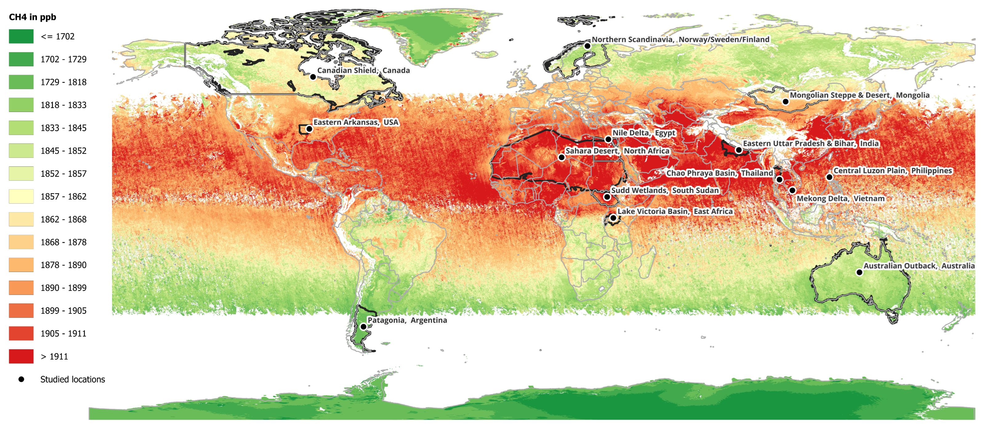
2.1. Study Area Selection

The study regions were selected based on scientific criteria and practical considerations to enable a robust and meaningful comparison of spatio-temporal methane emission patterns. Regions were classified into anthropogenic- and natural-emission categories based on their documented methane emission intensity from previous research, atmospheric monitoring programs, and global emission inventories (

Table 1. Summary of selected emission study regions.

Region Name	Dominant Land Use	Climate Zone	% Rice Cultivation Area	Population Density (Persons/km2)	References
Mekong Delta, Vietnam	Intensive rice agriculture	Humid tropical	65%	500+	[22]
Nile Delta, Egypt	Rice agriculture, urbanization	Mediterranean/subtropical	30%	1000+	[23]
Eastern Uttar Pradesh and Bihar, India	Rice agriculture	Humid subtropical	50%	900+	[24]
Chao Phraya Basin, Thailand	Rice agriculture, canal networks	Tropical monsoon	45%	800+	[25]
Lake Victoria Basin, East Africa	Natural wetlands, rice agriculture	Tropical savanna	10%	300+	[26]
Eastern Arkansas, USA	Mechanized rice agriculture	Humid subtropical	35%	50–100	[27]
Central Luzon Plain, Philippines	Irrigated rice agriculture	Tropical monsoon	55–60%	300–500	[28]
Patagonia, Argentina	Extensive grazing, natural grassland	Cold semi-arid	1%	<5	[29]
Mongolian Steppe and Desert, Mongolia	Sparse grassland, desert	Cold desert	0%	<2	[30]
Northern Scandinavia, Norway/Sweden/Finland	Boreal forest, tundra	Subarctic	0%	<5	[31]
Australian Outback, Australia	Arid shrubland, desert	Arid desert	0%	<1	[32]
Sahara Desert, North Africa	Desert, minimal vegetation	Hyper-arid desert	0%	<1	[33]
Canadian Shield, Canada	Boreal forest, lakes	Subarctic/boreal	0%	<2	[34]
Sudd Wetlands, South Sudan	Tropical wetlands, floodplains	Tropical savanna	<1%	10–30	[35]

; Figure 1). Anthropogenic-emission regions typically feature intensive agricultural activities (especially irrigated rice cultivation), dense livestock populations, or high human population density—all recognized as major methane sources [1,6]. Natural-emission regions, by contrast, are characterized by minimal anthropogenic activity, sparse vegetation, dry or cold climates, and low or high (natural wetlands) methane production [19]. To minimize the confounding effects of climatic variability, emission regions were paired within broadly similar climate zones (e.g., humid tropical zones for the Mekong Delta and Lake Victoria Basin vs. arid subtropical zones for the Sahara and Australian Outback). This strategy follows established best practices for comparative emission studies, where controlling for environmental factors improves the attribution of observed atmospheric signals to land use and emissions rather than to climate [20]. Only regions with reliable satellite data coverage were selected. Sentinel-5P TROPOMI data quality can be affected by persistent cloud cover, surface reflectance issues, and solar zenith angles [12]. Thus, areas where cloudiness or retrieval errors would systematically limit data availability were avoided. Selected regions display relatively homogeneous dominant land uses within the analysis boundaries, enhancing the interpretability of spatial methane patterns. For example, the Mekong Delta is dominated by flooded rice paddies, whereas the Mongolian Steppe is predominantly dry grassland with minimal human disturbance [21]. The study deliberately included regions from different continents and socio-environmental contexts (Asia, Africa, North America, South America, and Australia) to improve the generalizability of findings to broader global methane emission studies.

2.2. Satellite Data and Preprocessing

Atmospheric methane concentrations were obtained from the Level-3 XCH₄ data product of the TROPOspheric Monitoring Instrument (TROPOMI) onboard the Sentinel-5 Precursor satellite [12]. This dataset provides gridded, column-averaged dry air mole fractions of methane (XCH₄, in ppb) at approximately 0.1° × 0.1° spatial resolution and is made available through Google Earth Engine (GEE) via the COPERNICUS/S5P/OFFL/L3_CH4 collection [36]. The analysis covered the period from April 2019 to March 2025 and included only data where the qa_value (quality assurance flag) was ≥0.5, as recommended by the Sentinel-5P data documentation to ensure retrieval reliability. Methane data were aggregated into seasonal means, with seasons defined as Q1 (January–March), Q2 (April–June), Q3 (July–September), and Q4 (October–December). Seasonal aggregation reduces the impact of short-term gaps or retrieval variability, which is especially relevant in cloud-prone regions. Study region boundaries were defined using geographic masks created from administrative shapefiles, land-use datasets, and custom polygons drawn in GIS software. A custom polygon dataset was created (in QGIS 3.34, Gossau, Germany, 2021) to represent global regions with varying methane emission intensities, encompassing both low- and high-emission areas. Each region was represented by either a central polygon or point, and a uniform 50 km radius buffer was applied around this geometry to capture the surrounding area to ensure consistent spatial sampling. The polygon geometries were imported into GEE as FeatureCollections, and the regional mean of XCH₄ was calculated for each quarter using the reduceRegion() function with the mean reducer over the buffered geometry. The data were projected in EPSG:4326 (WGS84), and the result of each temporal interval was stored as a time series for each region. The resulting dataset consists of the quarterly mean CH₄ concentration in the atmospheric column values per region, which served as the basis for subsequent time series, trend, and multivariate analyses.

2.3. Trend and Seasonal Analysis

For each study region, the time series of monthly and seasonal mean XCH₄ values were generated. Long-term trends were quantified using the additive seasonal model. In time series analysis, an additive seasonal model assumes that the overall value of the series at any point in time can be decomposed into the sum of three distinct components:

$$Y_t=T_t+S_t+R_t$$

where

$Y_t$ is the observed value at time t;

$T_t$ is the trend component (long-term progression over time);

$S_t$ is the seasonal component (systematic, calendar-related variations);

$R_t$ is the residual component (random noise or unexplained variation).

The magnitude of the seasonal fluctuations, $S_t$, is assumed to be constant over time. The peaks and troughs due to seasonality do not increase or decrease as the overall level of the series changes. The seasonal variations in methane concentrations are relatively constant across time periods. There is no observable expansion or contraction in the amplitude of seasonal changes, despite changes in the underlying trend (i.e., the general growth or plateauing of XCH₄). Therefore, an additive structure accurately reflects the behavior of the methane time series. Trend slopes are expressed in parts per billion per quarter (ppb/quarter). Statistical significance was assessed using standard t-tests, with a significance threshold of p < 0.05. Cluster analysis and Principal Component Analysis (PCA) were used for exploratory purposes to identify similarities in temporal patterns across various global regions based on a time series of numerical values recorded quarterly from Q1 2020 to Q1 2025. To balance the dataset (not all seasons in all years were available), the dataset included all 14 geographical regions, each represented by a vector of 10 quarterly observations. The time periods analyzed were Q1 2020, Q2 2020, Q1 2021, Q4 2021, Q1 2022, Q4 2022, Q1 2023, Q1 2024, Q2 2024, and Q1 2025. Before clustering, the time series data for each region was standardized using z-score normalization (mean = 0; standard deviation = 1). The Euclidean distance was used to compute the dissimilarity between standardized time series. This metric calculates the straight-line distance between two multi-dimensional points and is appropriate after standardization. Agglomerative hierarchical clustering was applied using Ward’s linkage method. All statistical analyses were conducted using Python 3.10, Excel 2016, and Statistica 13 software. Visualizations were generated to highlight seasonal variability and regional differences in methane concentration dynamics.

3. Results

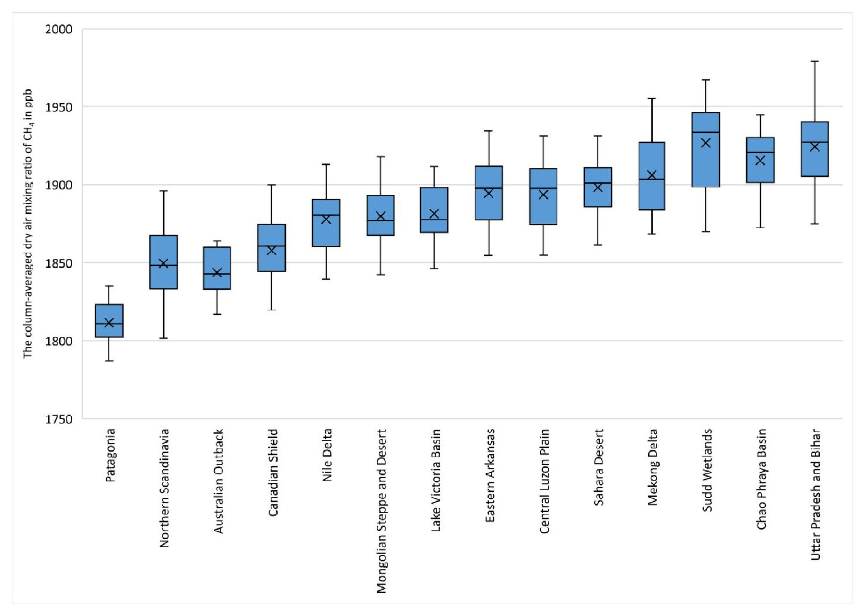
3.1. Overall Trends in Methane Concentration

Figure 2 visualizes the variation in XCH₄ for different global regions derived from the TROPOMI. Most regions have mean XCH₄ concentrations between 1850 and 1950 ppb, reflecting global average levels during recent years (from April 2019 to March 2025). Several regions exceed the upper end of this range, pointing to regional hotspots of methane emissions. Sudd Wetlands, Uttar Pradesh, and Bihar exhibit the highest median and upper quartile values, indicating persistent and increasing methane emissions. Wetland-related emissions (Sudd Wetlands) are a major natural methane source. Agricultural and anthropogenic activity (Uttar Pradesh and Bihar) especially includes rice cultivation and livestock. The Chao Phraya Basin and the Mekong Delta also show relatively high central values, aligning with their extensive wetland and agricultural activity. Patagonia and the Australian Outback display the lowest median XCH₄ levels. These regions are typically sparsely populated, with limited methane-producing activities. Their tight interquartile ranges and low whiskers suggest consistently low methane levels over time. Regions like the Canadian Shield, Northern Scandinavia, and the Mongolian Steppe and Desert present moderate medians but wide variability, reflecting the seasonal influences (e.g., snow cover and soil freeze–thaw cycles).

3.2. Trends and Seasonal Variations

The four graphs (Figure 3) present time series analyses of column-averaged methane concentrations (CH₄, in ppb) for different regions: Uttar Pradesh and Bihar, Australian Outback, Central Luzon Plain, and Patagonia. A strong positive trend is evident for Uttar Pradesh and Bihar, with methane concentrations increasing by approximately 2.4 ppb per quarter. Seasonal fluctuations around the trend are visible but do not significantly disrupt the upward trajectory. In the Australian Outback, a moderate increasing trend is observed, with methane levels rising by about 2.1 ppb per quarter. Methane levels remain relatively low (~1817–1870 ppb range), reflecting a stable low-emission environment with slow progressive change. In Central Luzon Plain, a strong positive trend is observed, which is almost identical to the slope of Uttar Pradesh and Bihar. Patagonia has a gentle positive trend with an increase of 1.8 ppb per quarter, the lowest trend among the four regions shown.

Table 2. The results of the additive seasonal model for the period of Q2 2019–Q1 2025. S1–S4—seasonal deviations from the trend for each quarter in ppb XCH₄; a—regression slope indicates the rate of XCH₄ increase per time unit (ppb/quarter); b—regression intercept, also known as the baseline XCH₄ level; R²—goodness of fit or how well the trend model explains the variability.

Region	S1 1 January–31 March	S2 1 April–30 June	S3 1 July–30 September	S4 1 October–31 December	a	b	R2	Seasonal Amplitude
Mekong Delta, Vietnam	2.85	−24.24	−27.49	13.86	1.56	1883.96	0.66	41.35
Nile Delta, Egypt	−11.27	−1.91	6.78	6.39	2.45	1847.29	0.92	18.05
Eastern Uttar Pradesh and Bihar, India	−16.31	−9.81	35.61	8.04	2.44	1892.51	0.85	51.92
Chao Phraya Basin, Thailand	−0.74	−6.9	22.95	−0.02	2.43	1888.58	0.69	29.85
Lake Victoria Basin, East Africa	8.26	−8.09	−8.77	17.21	1.95	1858.36	0.69	25.98
Eastern Arkansas, USA	−3.85	−2.87	−3.54	10.27	2.83	1859.11	0.69	14.12
Central Luzon Plain, Philippines	1.77	−0.31	−16.48	12.27	2.37	1862.93	0.86	28.75
Patagonia, Argentina	−2.88	−3.31	3.22	2.23	1.84	1788.48	0.93	6.53
Mongolian Steppe and Desert, Mongolia	−13.61	−8.56	11.85	10.33	2.15	1852.93	0.94	25.46
Northern Scandinavia, Norway/Sweden/Finland	6.08	0.86	−7.32	1.50	3.11	1810.8	0.82	13.40
Australian Outback, Australia	−5.53	3.29	2.03	0.20	2.14	1816.93	0.91	8.82
Sahara Desert, North Africa	−10.25	−5.02	8.48	10.31	2.11	1871.88	0.93	20.56
Canadian Shield, Canada	3.14	−6.99	−4.57	16.84	2.37	1829.53	0.70	23.83
Sudd Wetlands, South Sudan	−11.64	2.77	−3.90	11.47	3.00	1888.61	0.62	23.11

presents the results of the additive seasonal model for all regions. When seasonal deviations from the trend for each quarter are positive, XCH₄ is higher than the trend during that season, and negative values indicate that XCH₄ is lower than that. Anthropogenic methane emission regions generally have higher baseline methane levels (high b) and show distinct seasonality. The Mekong Delta has strong negative deviations in Q2 and Q3, as well as a recovery in Q4 with a moderate trend (a = 1.56) and a moderate R² (0.66), indicating some external variability. The Nile Delta has small seasonal effects and is more balanced. There is a strong positive trend (a = 2.45) with a very high R² (0.92) that dominates. Eastern Uttar Pradesh and Bihar have a strong peak in Q3 (probable harvest season), but the peak is low in Q1 and Q2 and has a strong positive trend (a = 2.44). The Chao Phraya Basin has a large Q3 peak. Otherwise, it is stable. XCH₄ in Lake Victoria Basin fluctuates: high in Q1 and Q4, with a lower mid-year value. Anthropogenic-emission regions have strong trends in methane concentration over time (typically a > 2), distinct seasonality, often with lower concentrations mid-year and recovery in Q4, and good model fits (R² between 0.66 and 0.92). The natural methane emission regions show lower baseline methane levels and often less pronounced seasonal effects. Patagonia, for example, has a very mild seasonality and moderate trend (a = 1.84) with a very high R² (0.93). For low-emission regions, trends are still present, but baseline levels are lower. Seasonality is weaker or more irregular. The difference between the highest seasonal effect and the lowest seasonal effect for low-emission regions was in the range from 6.53 to 25.46 with a mean of 17.39 ppb XCH₄. Respectively, for high-emission regions, the range was from 14.12 to 51.92 with a mean of 30.00 ppb XCH₄. Higher R² values indicate that trends explain most of the variance, except in regions with complex hydrological patterns (e.g., Sudd Wetlands). High-emission regions show a combination of rapidly increasing methane trends and strong seasonal cycles reflecting intensive biological and agricultural activities. Despite lower absolute levels, natural-emission regions often show clean trend patterns with minimal seasonal distortion, reflecting natural stability or long-term atmospheric transport patterns.

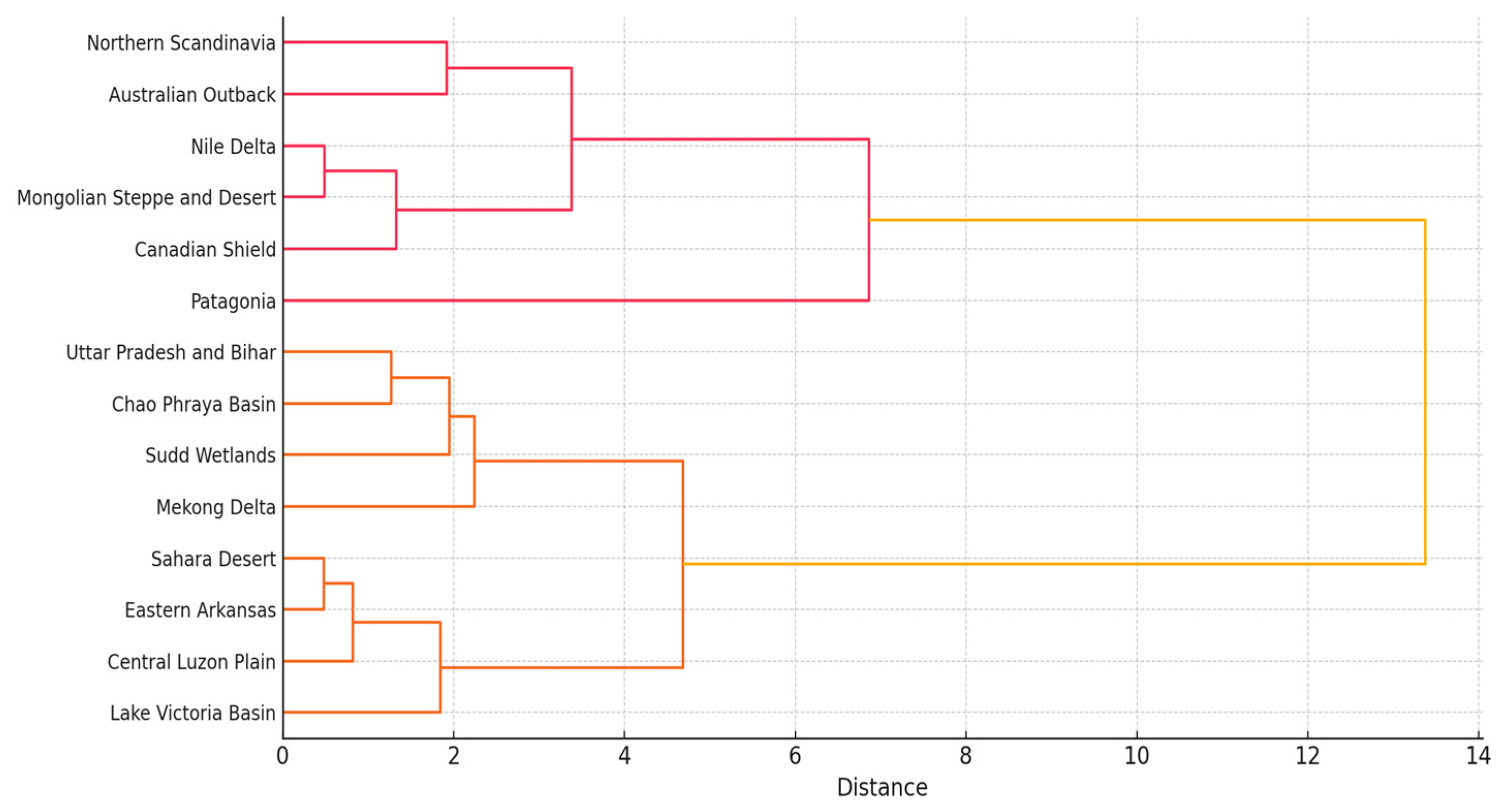
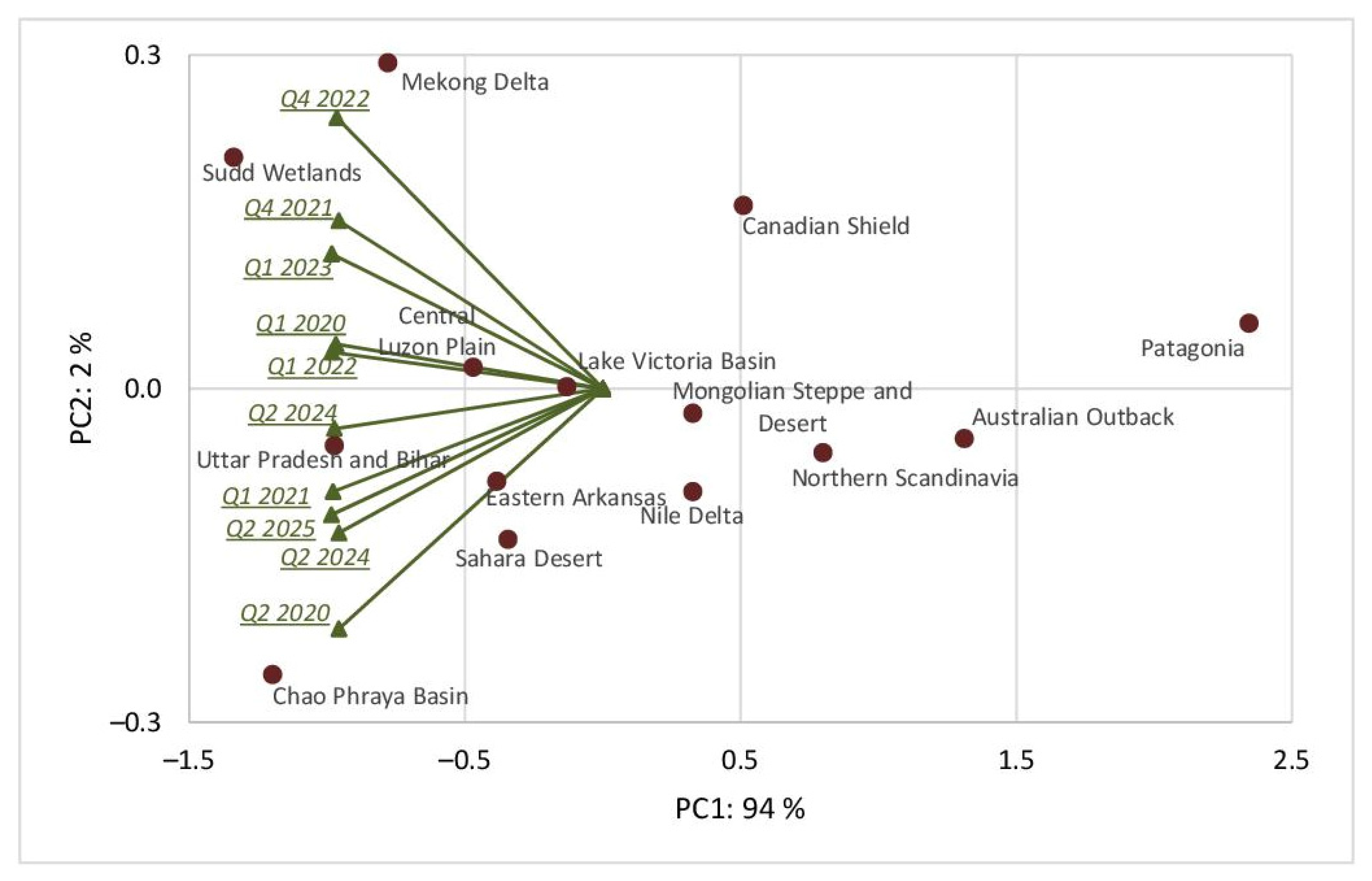
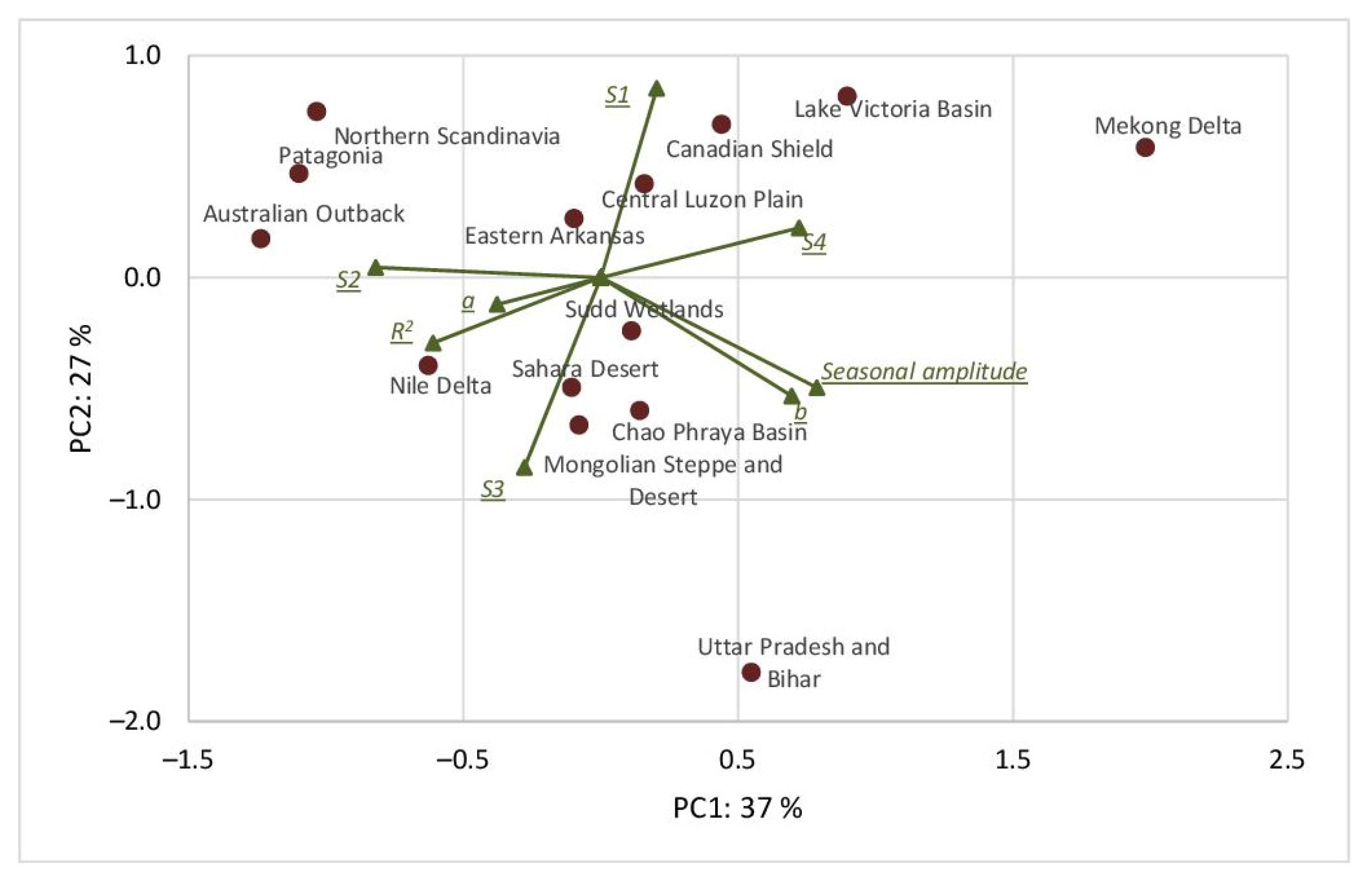
3.3. Multivariate Analysis of Regional Time Series

The cluster analysis aimed to group regions with similar temporal dynamics using hierarchical clustering. A dendrogram (Figure 4) was constructed to visualize the hierarchical relationships among regions. Each branch point (node) in the dendrogram represents a cluster merging event, with the node’s height reflecting the distance (dissimilarity) at which the merge occurred. Distinct clusters formed among regions with consistently high values or similar upward trends (e.g., Chao Phraya Basin, Sudd Wetlands, Uttar Pradesh, and Bihar). Another group includes regions with more moderate and stable values over time, such as the Canadian Shield, the Nile Delta, and the Mongolian Steppe and Desert. Patagonia and the Australian Outback appeared in the lower part of the dendrogram, indicating relatively lower and stable values with a pattern distinct from the more elevated profiles of other regions.

Chao Phraya Basin, Central Luzon Plain, Eastern Arkansas, Sudd Wetlands, Uttar Pradesh and Bihar, and the Mekong Delta regions with strong upward trends over time are grouped into one cluster, with the highest average trend slopes observed in the dataset. Regions in this cluster consistently exhibit high absolute values of the variable under study, suggesting persistent or intensifying pressures or development. The Australian Outback, Canadian Shield, Lake Victoria Basin, Mongolian Steppe and Desert, and the Nile Delta are in the second cluster. Northern Scandinavia and the Sahara Desert have moderate but consistent growth trends with mid-range slopes. These regions show lower variability and more conservative growth than the first cluster. The lowest absolute values in the dataset across all periods were for Patagonia, with a very slow upward trend and minimal changes quarter over quarter.

Figure 5 shows the results of PCA conducted on XCH₄ data across selected quarters between 2020 and 2025 (the same as for cluster analysis). The first principal component (PC1) explains 94% of the total variance, while the second principal component (PC2) accounts for an additional 2%. Together, PC1 and PC2 capture 96% of the variability, indicating that the two-dimensional space summarizes the structure within the data. Each point in the graph represents a specific region, such as the Mekong Delta, the Sahara Desert, or Patagonia. At the same time, the green vectors labeled with time markers (e.g., Q2 2020 and Q2 2024) trace the temporal dynamics of methane concentration patterns. The horizontal axis (PC1) represents the dominant gradient of regional methane variability. Regions such as the Chao Phraya Basin and Central Luzon Plain are located on the left side of the axis, indicating associations with relatively higher methane emissions linked to anthropogenic and wetland activities. In contrast, regions on the right side, such as Patagonia and the Australian Outback, represent areas with more stable and lower methane concentrations, often reflecting natural background levels rather than active emission hotspots. The vertical axis (PC2) captures minor seasonal or regional deviations much less influential than those described by PC1. Some slight vertical separation can be observed; for example, the Mekong Delta appears higher, while the Sahara Desert is lower, reflecting subtle differences likely associated with regional seasonality or local emission events. Regions characterized by intensive agricultural activity and natural wetlands, such as the Mekong Delta, Sudd Wetlands, and Chao Phraya Basin, tend to cluster on the left side of the PCA plot. This positioning highlights their dynamic behavior and significant contributions to atmospheric methane variability. In contrast, natural regions such as Patagonia, the Australian Outback, and Northern Scandinavia cluster towards the right, demonstrating their relatively stable and homogeneous methane concentration patterns. The green vectors connecting temporal labels suggest moderate seasonal dynamics. The clustering of time points around regions like the Central Luzon Plain and Lake Victoria Basin indicates that these areas exhibit relatively predictable seasonal variations in methane concentrations. In contrast, regions like the Sudd Wetlands and the Mekong Delta show more pronounced temporal shifts, highlighting their dynamic emission profiles. The PCA confirms that methane emission patterns are strongly differentiated between high-emission, dynamic regions and low-emission, stable regions. It emphasizes that regional typology, including land use and climatic conditions, plays a fundamental role in shaping the spatial and temporal distribution of atmospheric methane concentrations.

Figure 6 presents the results of PCA based on variables related to seasonal methane characteristics across different regions. PC1 explains 37% of the variance, while PC2 explains 27%, capturing 64% of the total variability in the dataset. This moderate level of explained variance suggests that multiple interacting factors influence the seasonal methane behavior in different regions. The horizontal axis (PC1) primarily separates regions based on broader seasonal amplitude and trend characteristics of methane. Regions like the Mekong Delta and the Lake Victoria Basin are associated with greater seasonal variation and stronger upward trends in methane concentrations. In contrast, regions such as the Australian Outback and Patagonia show more stable or weaker seasonal dynamics and lower trends in methane levels. The vertical axis (PC2) reflects a second dimension of variation related to specific seasonal phases. For example, Northern Scandinavia and Patagonia indicate subtle differences in seasonal cycle shapes compared to regions like Uttar Pradesh and Bihar. Regions near the origin, such as the Central Luzon Plain and Eastern Arkansas, exhibit more balanced behavior, combining moderate seasonal amplitudes and trends, without extremes in any particular direction. In contrast, regions farther from the origin, like the Mekong Delta and Uttar Pradesh and Bihar, show stronger and more distinctive seasonal or trend characteristics. The PCA reveals that seasonal regional methane dynamics and trends are not uniform. Wetland- and agriculture-dominated regions exhibit strong seasonal amplitudes and trends, while natural regions with lower human impact display more stable and subdued methane behaviors.

3.4. Exploring Drivers of Methane Variability

To better understand the drivers behind spatial and temporal variations in methane concentrations, we performed a Spearman correlation analysis between regional CH₄ indicators (mean and standard deviation) and key environmental and anthropogenic variables that were elaborated on based on the information from Table 1. The results are presented in Figure 7, with correlation coefficients and associated p-values in parentheses. High climate temperature shows the strongest statistically significant positive correlation with the CH₄ mean (ρ = 0.63, p = 0.02), suggesting that warmer regions are generally associated with elevated atmospheric methane concentrations. This aligns with the temperature sensitivity of microbial methanogenesis, particularly in tropical wetland and rice agriculture systems. The rice cultivation area is also significantly positively correlated with the CH₄ mean (ρ = 0.55, p = 0.04), reinforcing the known role of flooded rice paddies as major methane sources. The same was observed for human population density. Desert areas are negatively correlated with the CH₄ standard deviation (ρ = –0.58, p = 0.03), reflecting the stability and generally low emissions of arid landscapes, where biological methane production is minimal and seasonal variation is constrained. While high humidity shows moderate positive correlations with the CH₄ mean (ρ = 0.47), this association did not reach conventional significance thresholds (p > 0.05), though it suggests potentially meaningful trends that warrant further investigation. Forest and grassland coverage tend to correlate negatively with the CH₄ mean and standard deviation, though not significantly. This could indicate that more vegetated, less intensively managed regions may act as either methane-neutral or mildly suppressive environments.

4. Discussion

Based on satellite-derived XCH₄ data from Sentinel-5P, the present study reinforces and extends previous findings regarding global and regional methane dynamics, especially concerning agricultural land use. This study examines recent trends and spatial patterns in atmospheric methane concentrations from 2019 to 2025, with a focus on distinguishing the behavior of high- and low-emission regions. While the global distribution of methane concentrations has been well established in previous research (e.g., via GEOS-Chem simulations and TROPOMI observations) [37,38], the key objective here was to investigate how regional methane levels have changed in recent years, and what underlying drivers may explain the observed anomalies in different emission contexts.

The results demonstrate a clear spatial heterogeneity in the trend slope, seasonal amplitude, and temporal variability of methane concentrations, with significantly higher values associated with regions dominated by intensive rice cultivation and wetland systems, such as the Mekong Delta, Nile Delta, Eastern Uttar Pradesh and Bihar, and the Chao Phraya Basin. These findings are consistent with prior work by [39], who reported elevated atmospheric methane in rice-growing regions based on TROPOMI data and confirmed seasonal peaks related to agricultural practices. Our study observed that tropical deltas and wetlands continue to dominate global methane emissions. Seasonal analyses showed that methane concentrations generally peaked during Q3 (July–September) or Q4 (October–December), corresponding to the active rice-growing and wetland inundation periods. This observation aligns with prior studies indicating that anaerobic conditions during rice cultivation and natural wetland flooding favor microbial methane production [40,41]. Conversely, regions such as Patagonia, the Australian Outback, the Mongolian Steppe, and Northern Scandinavia exhibited lower baseline methane concentrations and more subdued seasonal fluctuations. These results parallel findings from [42,43] and recent [5] reports that natural arid or boreal environments generally act as low-methane-emission zones. However, gradual increases are visible and potentially linked to climate change effects such as permafrost thawing or changing soil respiration. The Canadian Shield stands out due to its moderate median XCH₄ values combined with wide seasonal variability, which can be interpreted as a signature of freeze–thaw cycles, wetland hydrology, and, possibly, permafrost degradation. Warmer seasonal temperatures can enhance anaerobic microbial activity in boreal wetlands [44], while thawing permafrost has been shown to release methane from previously frozen organic carbon stocks [45].

Correlation analyses supported the hypothesis that climate and land use are key co-drivers of observed trends. Mean CH₄ concentrations and standard deviations were positively associated with high temperature, human population density, and rice cultivation areas, confirming the role of tropical agriculture in intensifying emissions. Conversely, the standard deviation of CH₄ was negatively correlated with desert coverage, reflecting the suppressed seasonal variability of arid ecosystems. Methane’s production and accumulation are highly sensitive to temperature. Warmer conditions amplify microbial methanogenesis in flooded rice fields and wetlands [41] and may also trigger previously dormant emissions in cold or semi-arid regions. In northern latitudes, increasing thaw depth and longer growing seasons can lead to enhanced emissions [46], while rising fire frequency in savannahs and forests could increase episodic pulses of methane from biomass burning. Long-range transport and atmospheric circulation processes may contribute to increasing methane concentrations in arid and northern regions, particularly given the relatively long atmospheric lifetime of methane. These mechanisms offer plausible explanations for the gradual methane increases in low-emission regions observed in our dataset.

The hierarchical cluster analysis revealed three distinct groups of regions based on their temporal methane profiles: (1) dynamic, high-emission agricultural/wetland regions with strong upward trends; (2) moderate-growth regions characterized by climatic or ecological buffering; and (3) the highly stable low-emission environment represented by Patagonia. These patterns mirror previous clustering studies in atmospheric methane research [7], emphasizing the influence of socio-economic factors, land management, and environmental conditions on emission trajectories. The additive seasonal decomposition confirmed that seasonal effects are robust yet relatively constant in amplitude across the studied years, supporting the assumption of an additive model structure. Regions like the Mekong Delta showed moderate seasonal amplitudes with notable mid-year decreases. In contrast, Eastern Uttar Pradesh and Bihar displayed pronounced Q3 peaks coinciding with intensive agricultural activities [47]. PCA provided further confirmation of the dichotomy between high- and low-emission regions. High-emission agricultural zones clustered together and were strongly associated with seasonal amplitude and upward trends, while natural regions remained separated with more stable methane profiles. This differentiation suggests that targeted mitigation policies in agricultural and wetland regions are critical for achieving effective methane emission reductions. Compared to the results by [39,48], who reported a global increase of approximately 15 ppb/year in rice-dominated regions during 2019–2021, the present study found consistent or slightly lower growth rates (about 1.8–2.5 ppb per quarter). This similarity validates the reliability of TROPOMI-derived XCH₄ measurements and confirms that methane concentrations continue to rise in major emission hotspots despite various national and international mitigation efforts. Moreover, the moderate seasonal variability detected even in low-emission zones suggests that atmospheric methane burdens are increasingly influenced by long-range transport, a factor highlighted by [49] and seen in patterns observed over the Sahara and Canadian Shield. Taken together, the findings of this study stress the importance of region-specific monitoring and policy interventions. While rice agriculture and wetlands are well-established methane sources, their temporal dynamics and growth rates imply that mitigation measures must be adaptive to local land-use practices and seasonal emission patterns. Furthermore, the persistent increases even in low-emission regions call for enhanced atmospheric monitoring networks and the integration of satellite- and ground-based observations to disentangle local sources from transported methane signals. These findings suggest that recent anomalies in methane growth are not uniformly global but instead reflect a combination of land-use practices, climate forcing, and potentially regional feedback mechanisms. The observed trends underscore the need to focus mitigation efforts on agriculturally dominated regions while also improving monitoring in remote areas where changes may be less visible but still climatically relevant.

To explore common temporal structures across regions, we applied Principal Component Analysis (PCA) and hierarchical clustering. These techniques revealed clear separations between dynamic agricultural/wetland systems and stable natural regions. While PCA helped reduce dimensionality and visualize dominant patterns, we acknowledge its limitations. PCA assumes linear relationships and may not fully capture complex interactions or lagged responses. As such, PCA results were complemented by seasonal trend decomposition and correlation analysis for robustness. Additionally, we recognize that the TROPOMI CH₄ product, despite its transformative spatial coverage, carries inherent uncertainties related to retrieval quality, especially over high-albedo surfaces and regions with frequent cloud cover. We mitigated this by using only data with a qa_value ≥ 0.5 and by aggregating results seasonally to minimize short-term anomalies. Validation studies [17,18] confirm the reliability of the TROPOMI XCH₄ product across a range of conditions when properly filtered, although local validation with ground-based instruments (e.g., TCCON and NDACC) remains essential for uncertainty quantification.

The observed divergence in trend magnitudes and seasonal behaviors implies that recent methane growth is not globally uniform, but instead reflects a complex interplay of anthropogenic activity, climate forcing, and regional feedback. This has implications for both monitoring and mitigation. While agricultural areas remain the most obvious targets for methane reduction, our findings suggest that natural regions, especially boreal and subarctic zones, should not be neglected, as they may increasingly contribute to a warming climate.

5. Conclusions

This study provides a comparative analysis of methane emission dynamics across high- and low-emission regions between 2019 and 2025, utilizing satellite-derived XCH₄ observations from the Sentinel-5P TROPOMI mission. The results demonstrate that high-emission regions, primarily dominated by intensive rice cultivation and wetland systems, exhibited significantly greater seasonal variation in methane concentrations, with a mean seasonal amplitude of 30.00 ppb, compared to 17.39 ppb in low-emission regions. The highest intra-annual amplitudes were recorded in South and East Asia, particularly within major rice-producing regions such as the Mekong Delta, Eastern Uttar Pradesh and Bihar, and the Chao Phraya Basin. Across most of the studied regions, the highest XCH₄ concentrations were observed at the end of the year (Q4), while the lowest concentrations typically occurred in the first half of the year (Q1 or Q2). These temporal patterns align with agricultural cycles and seasonal wetland inundation periods, highlighting the critical role of land-use practices and hydrological variability in driving regional methane dynamics. The findings emphasize the value of integrating high-resolution satellite observations into greenhouse gas inventories and mitigation planning, particularly for targeting agricultural management practices in high-emission areas. Such integration is essential for improving the assessment of emissions through spatial and temporal resolution and supporting more effective policy interventions aimed at methane reduction. Nevertheless, some limitations must be acknowledged. Potential uncertainties arise from atmospheric transport effects, cloud contamination, and the mixed-source nature of atmospheric methane signals, which may complicate source attribution. Despite these challenges, the study confirms the strong capacity of satellite remote sensing, particularly TROPOMI, to detect, monitor, and characterize regional methane emission patterns over multiple years. This capability provides critical empirical support for developing targeted mitigation strategies and enhancing the overall accuracy of global greenhouse gas monitoring frameworks. Continued satellite-based monitoring, complemented by ground-based validation and atmospheric modeling efforts, will be crucial for tracking progress toward methane reduction goals and for better understanding the evolving dynamics of this potent greenhouse gas in a changing climate.

References

1. Intergovernmental Panel on Climate, C. Climate Change 2021—The Physical Science Basis: Working Group I Contribution to the Sixth Assessment Report of the Intergovernmental Panel on Climate Change; Cambridge University Press: Cambridge, UK, 2023. [Google Scholar]
2. Myhre, G.; Shindell, D.; Bréon, F.-M.; Collins, W.; Fuglestvedt, J.; Huang, J.; Koch, D.; Lamarque, J.-F.; Lee, D.; Mendoza, B.; et al. Anthropogenic and Natural Radiative Forcing. In Climate Change 2013—The Physical Science Basis; Cambridge University Press: Cambridge, UK, 2014; pp. 659–740. [Google Scholar]
3. Sonnemann, G.R.; Grygalashvyly, M. Global annual methane emission rate derived from its current atmospheric mixing ratio and estimated lifetime. Ann. Geophys. 2014, 32, 277–283. [Google Scholar] [CrossRef]
4. Etminan, M.; Myhre, G.; Highwood, E.J.; Shine, K.P. Radiative forcing of carbon dioxide, methane, and nitrous oxide: A significant revision of the methane radiative forcing. Geophys. Res. Lett. 2016, 43, 12614–12623. [Google Scholar] [CrossRef]
5. Forster, P.; Ramaswamy, V.; Artaxo, P.; Berntsen, T.; Betts, R.; Fahey, D.W.; Haywood, J.; Lean, J.; Lowe, D.C.; Myhre, G.; et al. Changes in Atmospheric Constituents and in Radiative Forcing. In Climate Change 2007: The Physical Science Basis. Contribution of Working Group I to the Fourth Assessment Report of the Intergovernmental Panel on Climate Change; Solomon, S., Qin, D., Manning, M., Chen, Z., Marquis, M., Averyt, K.B., Tignor, M., Miller, H.L., Eds.; Cambridge University Press: Cambridge, UK; New York, NY, USA, 2007. [Google Scholar]
6. Saunois, M.; Stavert, A.R.; Poulter, B.; Bousquet, P.; Canadell, J.G.; Jackson, R.B.; Raymond, P.A.; Dlugokencky, E.J.; Houweling, S.; Patra, P.K.; et al. The Global Methane Budget 2000–2017. Earth Syst. Sci. Data 2020, 12, 1561–1623. [Google Scholar] [CrossRef]
7. Nisbet, E.G.; Manning, M.; Dlugokencky, E.; Fisher, R.; Lowry, D.; Michel, S.; Myhre, C.L.; Platt, S.M.; Allen, G.; Bousquet, P. Very strong atmospheric methane growth in the 4 years 2014–2017: Implications for the Paris Agreement. Glob. Biogeochem. Cycles 2019, 33, 318–342. [Google Scholar] [CrossRef]
8. Schwietzke, S.; Sherwood, O.A.; Bruhwiler, L.M.P.; Miller, J.B.; Etiope, G.; Dlugokencky, E.J.; Michel, S.E.; Arling, V.A.; Vaughn, B.H.; White, J.W.C.; et al. Upward revision of global fossil fuel methane emissions based on isotope database. Nature 2016, 538, 88–91. [Google Scholar] [CrossRef] [PubMed]
9. Patra, P.K.; Saeki, T.; Dlugokencky, E.J.; Ishijima, K.; Umezawa, T.; Ito, A.; Aoki, S.; Morimoto, S.; Kort, E.A.; Crotwell, A.; et al. Regional Methane Emission Estimation Based on Observed Atmospheric Concentrations (2002–2012). J. Meteorol. Soc. Japan. Ser. II 2016, 94, 91–113. [Google Scholar] [CrossRef]
10. Rößger, N.; Sachs, T.; Wille, C.; Boike, J.; Kutzbach, L. Seasonal increase of methane emissions linked to warming in Siberian tundra. Nat. Clim. Change 2022, 12, 1031–1036. [Google Scholar] [CrossRef]
11. Hu, H.; Landgraf, J.; Detmers, R.; Borsdorff, T.; Aan De Brugh, J.; Aben, I.; Butz, A.; Hasekamp, O. Toward Global Mapping of Methane With TROPOMI: First Results and Intersatellite Comparison to GOSAT. Geophys. Res. Lett. 2018, 45, 3682–3689. [Google Scholar] [CrossRef]
12. Lorente, A.; Borsdorff, T.; Butz, A.; Hasekamp, O.; aan de Brugh, J.; Schneider, A.; Wu, L.; Hase, F.; Kivi, R.; Wunch, D.; et al. Methane retrieved from TROPOMI: Improvement of the data product and validation of the first 2 years of measurements. Atmos. Meas. Tech. 2021, 14, 665–684. [Google Scholar] [CrossRef]
13. Saad, K.M.; Wunch, D.; Toon, G.C.; Bernath, P.; Boone, C.; Connor, B.; Deutscher, N.M.; Griffith, D.W.T.; Kivi, R.; Notholt, J.; et al. Derivation of tropospheric methane from TCCON CH4 and HF total column observations. Atmos. Meas. Tech. 2014, 7, 2907–2918. [Google Scholar] [CrossRef]
14. De Mazière, M.; Thompson, A.M.; Kurylo, M.J.; Wild, J.D.; Bernhard, G.; Blumenstock, T.; Braathen, G.O.; Hannigan, J.W.; Lambert, J.C.; Leblanc, T.; et al. The Network for the Detection of Atmospheric Composition Change (NDACC): History, status and perspectives. Atmos. Chem. Phys. 2018, 18, 4935–4964. [Google Scholar] [CrossRef]
15. Alberti, C.; Hase, F.; Frey, M.; Dubravica, D.; Blumenstock, T.; Dehn, A.; Castracane, P.; Surawicz, G.; Harig, R.; Baier, B.C.; et al. Improved calibration procedures for the EM27/SUN spectrometers of the COllaborative Carbon Column Observing Network (COCCON). Atmos. Meas. Tech. 2022, 15, 2433–2463. [Google Scholar] [CrossRef]
16. Karion, A.; Sweeney, C.; Tans, P.; Newberger, T. AirCore: An Innovative Atmospheric Sampling System. J. Atmos. Ocean. Technol. 2010, 27, 1839–1853. [Google Scholar] [CrossRef]
17. Sha, M.K.; Langerock, B.; Blavier, J.F.L.; Blumenstock, T.; Borsdorff, T.; Buschmann, M.; Dehn, A.; De Mazière, M.; Deutscher, N.M.; Feist, D.G.; et al. Validation of methane and carbon monoxide from Sentinel-5 Precursor using TCCON and NDACC-IRWG stations. Atmos. Meas. Tech. 2021, 14, 6249–6304. [Google Scholar] [CrossRef]
18. Lindqvist, H.; Kivimäki, E.; Häkkilä, T.; Tsuruta, A.; Schneising, O.; Buchwitz, M.; Lorente, A.; Martinez Velarte, M.; Borsdorff, T.; Alberti, C.; et al. Evaluation of Sentinel-5P TROPOMI Methane Observations at Northern High Latitudes. Remote Sens. 2024, 16, 2979. [Google Scholar] [CrossRef]
19. Kirschke, S.; Bousquet, P.; Ciais, P.; Saunois, M.; Canadell, J.G.; Dlugokencky, E.J.; Bergamaschi, P.; Bergmann, D.; Blake, D.R.; Bruhwiler, L.; et al. Three decades of global methane sources and sinks. Nat. Geosci. 2013, 6, 813–823. [Google Scholar] [CrossRef]
20. Bloom, A.A.; Bowman, K.W.; Lee, M.; Turner, A.J.; Schroeder, R.; Worden, J.R.; Weidner, R.; McDonald, K.C.; Jacob, D.J. A global wetland methane emissions and uncertainty dataset for atmospheric chemical transport models (WetCHARTs version 1.0). Geosci. Model Dev. 2017, 10, 2141–2156. [Google Scholar] [CrossRef]
21. Bousquet, P.; Ciais, P.; Miller, J.B.; Dlugokencky, E.J.; Hauglustaine, D.A.; Prigent, C.; Van der Werf, G.R.; Peylin, P.; Brunke, E.G.; Carouge, C.; et al. Contribution of anthropogenic and natural sources to atmospheric methane variability. Nature 2006, 443, 439–443. [Google Scholar] [CrossRef]
22. Tong, Y.D. Rice intensive cropping and balanced cropping in the Mekong Delta, Vietnam—Economic and ecological considerations. Ecol. Econ. 2017, 132, 205–212. [Google Scholar] [CrossRef]
23. Radwan, T.M.; Blackburn, G.A.; Whyatt, J.D.; Atkinson, P.M. Dramatic loss of agricultural land due to urban expansion threatens food security in the Nile Delta, Egypt. Remote Sens. 2019, 11, 332. [Google Scholar] [CrossRef]
24. Kumar, N.; Chhokar, R.; Meena, R.; Kharub, A.; Gill, S.; Tripathi, S.; Gupta, O.; Mangrauthia, S.; Sundaram, R.; Sawant, C. Challenges and opportunities in productivity and sustainability of rice cultivation system: A critical review in Indian perspective. Cereal Res. Commun. 2021, 50, 573–601. [Google Scholar] [CrossRef]
25. Molle, F. Scales and power in river basin management: The Chao Phraya River in Thailand 1. Geogr. J. 2007, 173, 358–373. [Google Scholar] [CrossRef]
26. Were, D.; Kansiime, F.; Fetahi, T.; Hein, T. Carbon dioxide and methane fluxes from a tropical freshwater wetland under natural and rice paddy conditions: Implications for climate change mitigation. Wetlands 2021, 41, 52. [Google Scholar] [CrossRef]
27. Humphreys, J.; Brye, K.R.; Rector, C.; Gbur, E.E. Methane emissions from rice across a soil organic matter gradient in Alfisols of Arkansas, USA. Geoderma Reg. 2019, 16, e00200. [Google Scholar] [CrossRef]
28. Silva, J.V.; Reidsma, P.; Velasco, M.L.; Laborte, A.G.; van Ittersum, M.K. Intensification of rice-based farming systems in Central Luzon, Philippines: Constraints at field, farm and regional levels. Agric. Syst. 2018, 165, 55–70. [Google Scholar] [CrossRef]
29. Busso, C.A.; Fernández, O.A. Arid and semiarid rangelands of Argentina. In Climate Variability Impacts on Land Use and Livelihoods in Drylands; Springer: Berlin/Heidelberg, Germany, 2018; pp. 261–291. [Google Scholar]
30. Pfeiffer, M.; Dulamsuren, C.; Jäschke, Y.; Wesche, K. Grasslands of China and Mongolia: Spatial extent, land use and conservation. In Grasslands of the World: Diversity, Management and Conservation; Routledge: London, UK, 2018; pp. 168–196. [Google Scholar]
31. Virtanen, R.; Oksanen, L.; Oksanen, T.; Cohen, J.; Forbes, B.C.; Johansen, B.; Käyhkö, J.; Olofsson, J.; Pulliainen, J.; Tømmervik, H. Where do the treeless tundra areas of northern highlands fit in the global biome system: Toward an ecologically natural subdivision of the tundra biome. Ecol. Evol. 2016, 6, 143–158. [Google Scholar] [CrossRef]
32. Finn, D.; Dalal, R.; Klieve, A. Methane in Australian agriculture: Current emissions, sources and sinks, and potential mitigation strategies. Crop Pasture Sci. 2014, 66, 1–22. [Google Scholar] [CrossRef]
33. Prăvălie, R. Drylands extent and environmental issues. A global approach. Earth-Sci. Rev. 2016, 161, 259–278. [Google Scholar] [CrossRef]
34. Price, D.T.; Alfaro, R.I.; Brown, K.; Flannigan, M.D.; Fleming, R.A.; Hogg, E.H.; Girardin, M.P.; Lakusta, T.; Johnston, M.; McKenney, D.W. Anticipating the consequences of climate change for Canada’s boreal forest ecosystems. Environ. Rev. 2013, 21, 322–365. [Google Scholar] [CrossRef]
35. Rebelo, L.-M.; Senay, G.B.; McCartney, M.P. Flood pulsing in the Sudd wetland: Analysis of seasonal variations in inundation and evaporation in South Sudan. Earth Interact. 2012, 16, 1–19. [Google Scholar] [CrossRef]
36. Gorelick, N.; Hancher, M.; Dixon, M.; Ilyushchenko, S.; Thau, D.; Moore, R. Google Earth Engine: Planetary-scale geospatial analysis for everyone. Remote Sens. Environ. 2017, 202, 18–27. [Google Scholar] [CrossRef]
37. Drinkwater, A.; Palmer, P.I.; Feng, L.; Arnold, T.; Lan, X.; Michel, S.E.; Parker, R.; Boesch, H. Atmospheric data support a multi-decadal shift in the global methane budget towards natural tropical emissions. Atmos. Chem. Phys. 2023, 23, 8429–8452. [Google Scholar] [CrossRef]
38. Yu, X.; Millet, D.B.; Henze, D.K.; Turner, A.J.; Delgado, A.L.; Bloom, A.A.; Sheng, J. A high-resolution satellite-based map of global methane emissions reveals missing wetland, fossil fuel, and monsoon sources. Atmos. Chem. Phys. 2023, 23, 3325–3346. [Google Scholar] [CrossRef]
39. Kozicka, K.; Gozdowski, D.; Wójcik-Gront, E. Spatial-Temporal Changes of Methane Content in the Atmosphere for Selected Countries and Regions with High Methane Emission from Rice Cultivation. Atmosphere 2021, 12, 1382. [Google Scholar] [CrossRef]
40. Kumaraswamy, S.; Kumar Rath, A.; Ramakrishnan, B.; Sethunathan, N. Wetland rice soils as sources and sinks of methane: A review and prospects for research. Biol. Fertil. Soils 2000, 31, 449–461. [Google Scholar] [CrossRef]
41. Conrad, R. Methane production in soil environments—Anaerobic biogeochemistry and microbial life between flooding and desiccation. Microorganisms 2020, 8, 881. [Google Scholar] [CrossRef]
42. Sabrekov, A.F.; Runkle, B.R.; Glagolev, M.V.; Terentieva, I.E.; Stepanenko, V.M.; Kotsyurbenko, O.R.; Maksyutov, S.S.; Pokrovsky, O.S. Variability in methane emissions from West Siberia’s shallow boreal lakes on a regional scale and its environmental controls. Biogeosciences 2017, 14, 3715–3742. [Google Scholar] [CrossRef]
43. Laanbroek, H.J. Methane emission from natural wetlands: Interplay between emergent macrophytes and soil microbial processes. A mini-review. Ann. Bot. 2010, 105, 141–153. [Google Scholar] [CrossRef]
44. Kotsyurbenko, O.; Glagolev, M.; Merkel, A.; Sabrekov, A.; Terentieva, I. Methanogenesis in soils, wetlands, and peat. In Biogenesis of Hydrocarbons; Springer: Berlin/Heidelberg, Germany, 2019; pp. 211–228. [Google Scholar]
45. Miesner, F.; Overduin, P.P.; Grosse, G.; Strauss, J.; Langer, M.; Westermann, S.; Schneider von Deimling, T.; Brovkin, V.; Arndt, S. Subsea permafrost organic carbon stocks are large and of dominantly low reactivity. Sci. Rep. 2023, 13, 9425. [Google Scholar] [CrossRef]
46. Bao, T.; Xu, X.; Jia, G.; Billesbach, D.P.; Sullivan, R.C. Much stronger tundra methane emissions during autumn freeze than spring thaw. Glob. Change Biol. 2021, 27, 376–387. [Google Scholar] [CrossRef]
47. Zhang, Y.; Fang, S.; Chen, J.; Lin, Y.; Chen, Y.; Liang, R.; Jiang, K.; Parker, R.J.; Boesch, H.; Steinbacher, M. Observed changes in China’s methane emissions linked to policy drivers. Proc. Natl. Acad. Sci. USA 2022, 119, e2202742119. [Google Scholar] [CrossRef] [PubMed]
48. Kozicka, K.; Orazalina, Z.; Gozdowski, D.; Wójcik-Gront, E. Evaluation of temporal changes in methane content in the atmosphere for areas with a very high rice concentration based on Sentinel-5P data. Remote Sens. Appl. Soc. Environ. 2023, 30, 100972. [Google Scholar] [CrossRef]
49. Lunt, M.F.; Palmer, P.I.; Feng, L.; Taylor, C.M.; Boesch, H.; Parker, R.J. An increase in methane emissions from tropical Africa between 2010 and 2016 inferred from satellite data. Atmos. Chem. Phys. 2019, 19, 14721–14740. [Google Scholar] [CrossRef]
Figure 1. Global map of average column-averaged methane concentrations (XCH4, in parts per billion) for the period of April 2019 to March 2025, which were derived from the Sentinel-5P TROPOMI Level-3 product (OFFL/L3_CH4). The spatial resolution of the gridded dataset is 0.1° × 0.1°. Black circles indicate the geographic centers of the 14 study regions. Color shading represents mean XCH4 values over land, with a discrete scale indicating concentration ranges. Oceanic areas are included for context but contain substantially fewer valid retrievals due to low surface reflectance and cloud contamination.
Atmosphere 16 00670 g001
Figure 2. Boxplot of column-averaged methane concentrations (XCH4, in ppb) for selected global regions based on seasonal data for the period of April 2019–March 2025. Each box represents the interquartile range—from the 25th to the 75th percentile—of XCH4 values across multiple time points, with the horizontal line denoting the median and whiskers indicating minimum and maximum values. The “×” symbol marks the mean value.
Atmosphere 16 00670 g002
Figure 3. Time series analyses of column-averaged methane concentrations (CH4, in ppb) for selected global regions based on seasonal mean values from Q2 2019 to Q4 2025. Each panel represents a different region. Blue points correspond to quarterly XCH4 values derived from TROPOMI satellite data. The orange line represents the fitted additive trend line obtained from a seasonal decomposition model. The regression equation and the R2 value are provided to quantify the strength and slope of the long-term trend. The y-axis shows methane concentration in ppb, while the x-axis represents sequential calendar quarters.
Atmosphere 16 00670 g003
Figure 4. The hierarchical relationships among regions. Each branch point (node) in the dendrogram represents a cluster merging event, with the node’s height reflecting the distance (dissimilarity—Euclidean distance) at which the merge occurred.
Atmosphere 16 00670 g004
Figure 5. The biplot of a Principal Component Analysis (PCA) conducted on regional methane concentration (XCH4) data across selected quarters between 2020 and 2025.
Atmosphere 16 00670 g005
Figure 6. The biplot of a Principal Component Analysis (PCA) of seasonal regional methane (XCH4) characteristics and trend parameters. The green vectors labeled S1, S2, S3, and S4 correspond to the seasonal effects in each quarter, while vectors labeled a, b, and R2 reflect the regression coefficients, intercepts, and model fit parameters for the seasonal regression models. The vector labeled “Seasonal amplitude” suggests an overall gradient related to the strength of seasonal methane variability.
Atmosphere 16 00670 g006
Figure 7. Heatmap showing the Spearman correlations between the CH4 mean and CH4 standard deviation (SD) and the selected environmental and land-use variables. Each cell includes both the correlation coefficient and its p-value in parentheses.
Atmosphere 16 00670 g007