A Review of Offshore Methane Quantification Methodologies

Abstract

Since pre-industrial times, anthropogenic methane emissions have increased and are partly responsible for a changing global climate. Natural gas and oil extraction activities are one significant source of anthropogenic methane. While methods have been developed and refined to quantify onshore methane emissions, the ability of methods to directly quantify emissions from offshore production facilities remains largely unknown. Here, we review recent studies that have directly measured emissions from offshore production facilities and critically evaluate the suitability of these measurement strategies for emission quantification in a marine environment. The average methane emissions from production platforms measured using downwind dispersion methods were 32 kg h⁻¹ from 188 platforms; 118 kg h⁻¹ from 104 platforms using mass balance methods; 284 kg h⁻¹ from 151 platforms using aircraft remote sensing; and 19,088 kg h⁻¹ from 10 platforms using satellite remote sensing. Upon review of the methods, we suggest the unusually large emissions, or zero emissions observed could be caused by the effects of a decoupling of the marine boundary layer (MBL). Decoupling can happen when the MBL becomes too deep or when there is cloud cover and results in a stratified MBL with air layers of different depths moving at different speeds. Decoupling could cause: some aircraft remote sensing observations to be biased high (lower wind speed at the height of the plume); the mass balance measurements to be biased high (narrow plume being extrapolated too far vertically) or low (transects miss the plume); and the downwind dispersion measurements much lower than the other methods or zero (plume lofting in a decoupled section of the boundary layer). To date, there has been little research on the marine boundary layer, and guidance on when decoupling happens is not currently available. We suggest an offshore controlled release program could provide a better understanding of these results by explaining how and when stratification happens in the MBL and how this affects quantification methodologies.

1. Introduction

Globally, it is reported that 29% of all crude oil is produced offshore while 28% of natural gas is produced offshore with an average of 27 million barrels oil per day and 17.5 million barrels per day equivalent of natural gas (1.05 trillion cubic meters per year or 37 Tcf NG) [1,2,3]. Saudia Arabia and Brazil are the largest offshore producers, extracting 13% and 12% of the total offshore crude oil globally, respectively, and combined with Mexico, Norway and the USA collectively extract 43% of the global offshore crude oil. The largest production regions are the Persian Gulf, the Gulf of Mexico, the West Coast of Africa, and the North Sea.

Offshore platforms or rigs are used to extract oil and gas from beneath the seabed and typically comprise a large working deck at a safe distance above the ocean surface that is supported by either legs reaching to the seafloor or a buoyant vessel tethered to the sea floor. Rigs are primarily used for drilling and temporary extraction while platforms are designed for long-term extraction and production operations. Platform types include Fixed, Spar, Semi-submersible, Tension leg, Compliant tower, or Floating Production, Storage and Offloading (FPSO) facilities with most measurements occurring in the Gulf of Mexico [4,5,6,7,8].

Fixed platforms, including fixed leg, well protector and caisson types, are generally held up by legs fixed into the ocean floor [9]. Fixed leg and well protector facilities typically use tubular steel while caissons have submersible oil storage tanks running to the seabed. For all types, the subsurface infrastructure supports the deck where processing occurs. Fixed platforms have long life cycles, designed to last at least 25 years, and deployed in water depths up to 1700 ft [9]. According to the Bureau of Safety and Environmental Enforcement (BSEE) data, fixed platforms in the Gulf of Mexico are typically unmanned and in near-shore (<150 nm), relatively shallow (<6000 ft) waters. These facilities are typically older, lower-producing platforms with less processing equipment (typically separators only), and produced oil and gas is piped to shore [10]. In the Gulf of Mexico, 95% of the operating platforms are fixed platforms.

The remaining 5% of platforms in the Gulf of Mexico are newer, work farther offshore in deeper water, have higher production rates, more processing equipment, can store oil, and have power generation capabilities. Spar platforms are fixed on a large vertical cylinder which is used for storing produced liquids and tether to the seabed [9]. The deck of a semi-submersible platform is attached to the top of submersible pontoons which are kept in place by seabed anchors and are used to keep the platform on station. Tension leg platforms use four air-filled pillars connected by a square pontoon structure that is fastened to the ocean floor, which allows the platform to resist both vertical and rotational forces. Compliant tower platforms are connected to slender supports fixed to the seabed which allows the structure to sway with the motion of the ocean making them more stable in the stronger currents found in deeper water. The FPSOs are fitted with all equipment needed to process and store oil until it is offloaded by a tanker and comprise a vessel that is moored to the seabed while receiving oil and gas from subsea wells. On average the newer facilities produce 3500 kg CH₄ facility⁻¹ h⁻¹ while fixed leg facilities produce an average of 480 kg CH₄ facility⁻¹ h⁻¹ [10]. Fixed platforms are much less complex, with fewer pieces of processing equipment, and most facilities have no oil storage on site, no gas compression or electricity generation.

Even though there has been a great deal of recent activity quantifying methane emissions from onshore oil and gas production activities [11,12,13,14,15,16,17], there has been less attention given to quantifying methane emissions from similar endeavors offshore despite contributing nearly one-third of global oil and gas production [1]. Methane is a potent greenhouse gas (global warming potential 25 times higher than carbon dioxide over 100 years), has been linked with a changing global climate, and has been identified as a key gas for mitigation for short-term climate benefits [18,19,20,21]. In recent years, many methods have been developed and tuned to quantify methane emissions from onshore oil and gas production facilities. These include component-level measurements [22,23,24], downwind dispersion approaches [16,25,26,27], tracer-flux methods [28], mass balance [29] and using remote sensing from aircraft [30,31,32] and satellite [33,34] platforms. Each of these methods and its associated advantages, shortcomings and assumptions are described in Section 2 below. In most cases it is assumed that methods can be directly applied to measure offshore emissions; however, it is currently unclear if this is correct.

One key question is whether it can be adapted to account for differences between the terrestrial and marine environments. The most obvious methodological adaptation for offshore has been for remote sensing platforms that measure the absorbance of solar infra-red (IR) radiation as it passes through a methane plume. On land, flat surfaces and the absence of other IR absorbent chemicals make this relatively straight forward. In the marine environment, waves obfuscate reflectance and water absorbs IR meaning that a sun-glint method was developed to measure the absorption of IR at large angles of specular reflection [8,35,36,37,38]. Despite being used to quantify offshore methane emissions, the sun-glint approach has never been validated in a controlled-release experiment.

Another consideration of method applicability is whether it accounts for any differences in the boundary layer, i.e., the layer of the atmosphere closest to the surface of the Earth [39]. While the terrestrial boundary layer is relatively deep, dry and convective by day and shallow, dry and stratified at night, the marine boundary layer is typically always shallow, cool and moist (typical near-surface RH of 75–100%) [40,41]. Also, when the marine boundary layer depth is less than one kilometer, it is generally well-mixed and capped by a strong temperature inversion [42], but when it deepens or there is enough radiative heating of the cloud layer, the cloudy layer can decouple from the oceanic moisture source which reduces the mixing of air (partial or total) through the full depth leading to stratification [43]. Stratification could affect any method that assumes that the plume disperses in a uniformly conical shape or that the wind speed at a given height can be derived from a logarithmic wind profile.

To investigate if the methods currently used to measure methane emissions from offshore oil and gas production facilities generate realistic values, we will conduct a review of these methods and discuss any possible sources of measurement bias. Specifically, we will look into the following: 1. describe all methods that could be used to quantify offshore emissions; 2. review all published studies that have reported the size of emissions from offshore; 3. generate average emissions for methods that have measured a significant number of facilities; 4. suggest any possible causes of bias or uncertainty in the methodologies.

2. Materials and Methods

Several methods have been used to quantify emissions from offshore facilities. Typically, methods use measured methane concentrations and meteorology to infer the emission rate. Below are five method descriptions that have been used and include the following: component-level measurements; downwind dispersion approaches; tracer-flux; mass balance; and remote sensing approaches. For each method, a description of the approach is given along with any assumptions made. Emission rates have also been included to illustrate the typical size of emissions these methods have been used to measure in the past.

2.1. Component Level Measurements

Total site emission is inferred from the sum of emissions from individual sources measured at the component level. This method has been used in the past to report total facility fugitive emissions as part of a leak detection and repair program as part of the Gulf-wide Emission Inventory Study published by the US Bureau of Ocean Energy Management (BOEM) [44]. In most cases, optical gas imaging (OGI) cameras are used to locate the leak and a Hi-Flow sampler is used to measure the emission rates [45,46]. These instruments are commercially available and comprise a bag fixed over the source, the gas is then carried in a flow of air at a high flow rate to a methane sensor [46]. Hi-Flow samplers are typically used to quantify emissions between 50 g CH₄ h⁻¹ and 9 kg CH₄ h⁻¹ to an accuracy of ±10% [47]. Hi-Flow samplers are often used with OGI cameras which are first used to find the leak and then used to ensure all the gas is drawn into the sampler bag.

The advantages of this method are that it is relatively inexpensive as instrumentation is lower cost, relatively little training is required to make adequate measurements, and the direct measurements mean the emission estimate of the sources has a relatively small uncertainty. However, this method is very time-consuming, and sources may be missing if they are hard to reach or the emissions are intermittent. Component-level emission estimates are typically biased low and likely an underestimate or a lower bound of the actual emissions. The major assumption is that all emission sources have been accounted for and measured.

2.2. Downwind Dispersion Approach—Gaussian Plume Inverse Approach

Gaussian plume-based approaches use methane concentration measurements coupled with meteorological data to infer the emission rate from the facility [48,49,50]. The emission rate of the gas (Q, g s⁻¹) can be calculated from a methane concentration (Χ, g m⁻³) measured at a distance downwind of the source (x, m), the lateral distance from the center of the plume (y, m), the measurement height (z, m), wind speed (u, m s⁻¹), height of the source (h_s, m), height of the boundary layer (h, m) and the Pasquill Gifford Stability Class (Equation (1)). The Pasquill Gifford Stability Class is used to determine the standard deviations of the lateral (σ_y, m) and vertical (σ_z, m) mixing ratio distributions [48] using a look-up table [51]. Site-specific dispersion coefficients can also be generated by measuring turbulence using a high-frequency sonic anemometer.

$$X\left(x,y,z\right)={\displaystyle \frac{Q}{2\pi u{\sigma }_y{\sigma }_z}}{e}^{{\displaystyle \frac{-y^2}{{{2\sigma }_y}^2}}}\left(e^{{\displaystyle \frac{-{\left(z-h_s\right)}^2}{{{2\sigma }_z}^2}}}+e^{{\displaystyle \frac{-{\left(z+h_s\right)}^2}{{{2\sigma }_z}^2}}}+e^{{\displaystyle \frac{-{\left(z-2h+h_s\right)}^2}{{{2\sigma }_z}^2}}}+e^{{\displaystyle \frac{-{\left(z+2h-h_s\right)}^2}{{{2\sigma }_z}^2}}}+e^{{\displaystyle \frac{-{\left(z-2h-h_s\right)}^2}{{{2\sigma }_z}^2}}}\right)$$

(1)

The assumptions made by the Gaussian plume inverse method are as follows: 1. the source is emitting CH₄ at a constant rate; 2. the mass of methane is conserved when reflected at the surface of the ground or the top of the boundary layer; 3. wind speed and vertical eddy diffusivity are constant with time; 4. there is uniform vertical mixing; 5. the terrain is relatively flat between source and detector; 6. the distance between the source and detector is more than 100 m; 7. the emission is a point source; 8. all emissions are detectable from the measurement location. In a stratified atmosphere, it is likely that assumptions 2, 3, 4, and 8 are violated.

The advantages of this method are that the implementation of the equation is relatively straight-forward, the equation always gives an answer even when an assumption is violated, and emissions can be calculated in real time. This is the only method that has been validated by measurements made in a marine environment and is in good agreement with tracer flux [52,53]. The disadvantages are that all micrometeorology (particularly roughness length) cannot be fully accounted for in the equation and this approach does not account for air movement in complex aerodynamic environments.

2.3. Tracer Flux

The tracer flux method assumes that a tracer gas released next to a methane source will behave similarly as it encounters aerodynamic obstructions; therefore, the ratio of tracer to methane measured downwind can be used to infer the methane release rate [28,54]. The tracer gas with a known emission rate (Q_t, g m⁻² s⁻¹) is released next to an unknown methane source. Methane (X_m, g m⁻³) and tracer gas concentrations (X_t, g m⁻³) are measured downwind and the methane emission rate of the unknown source (Q, g m⁻² s⁻¹) is calculated from the ratio of concentrations (Equation (2)) [28]. To improve accuracy and ensure the correct plume is being observed, two tracer gas emissions can be used on either side of the unknown methane emission source [55]. Nitrous oxide and acetylene are often used as tracers for oil and gas operations. The uncertainty of quantification varies with wind conditions but is estimated at ±25% [28,56,57].

$$Q=Q_t.{\displaystyle \frac{{{\displaystyle \int }}_{y_{min}\left(p\right)}^{y_{max}\left(p\right)}\left[X_{plume}\left(p\right)-X_{bgnd}\left(p\right)\right] d{y}_p}{{{\displaystyle \int }}_{y_{min}\left(t\right)}^{y_{max}\left(t\right)}\left[X_{plume}\left(t\right)-X_{bgnd}\left(t\right)\right] d{y}_t}}$$

(2)

The main assumptions of this method are that the tracer and methane have the same dispersion properties, the tracer and methane have attained the same dilution factor at a distance downwind, and the source does not emit any of the tracer gas. The advantages are it does not require meteorological measurements or dispersion assumptions, but it does require at least two mobile ppb-level gas analyzers which increase the level of operational complexity and the cost. The tracer gas has to be collocated with the methane source, and this can be a challenge when the source cannot be reached or in case of multiple emitting point sources. Tracer gas cylinders are also required, which can be difficult in controlled areas.

2.4. Mass Balance Approaches

Emissions from a source (Q, g s⁻¹; Equation (3)) are calculated from the difference in upwind (X_b, g m⁻³) and downwind (X_e, g m⁻³) methane concentrations multiplied by the wind speed at that height (u, m s⁻¹) integrated over the plume width (y, m) and height (z, m) upwind (X_b, g m⁻³) [54]. Mass balance measurements can be conducted using a point sensor or using line-averaged sensors [54,58]. Transects of the plume must be measured from below to above the plume, as should the wind speed.

$$Q={{\displaystyle \int }}_0^z{{\displaystyle \int }}_{-y}^y{u}_z\left(X_{e,y,z}-X_{b,y,z}\right) dy dz$$

(3)

The major assumptions of the mass balance are as follows: 1. two-dimensional downwind measurement transects extending above, below and beyond the lateral extent of the plume from sea level to the top of the boundary layer; 2. horizontal scans are close enough together to detail size and shape of the plume, i.e., not too far apart; 3. the plume between horizontal scans is similar enough to extrapolate between transects; 4. the wind speed is known at each measurement height; 5. consecutive horizontal scans are performed fast enough to account for any vertical movement of the plume. The major advantage of the method is that the plume can be visualized; however, this method requires an analyzer to measure above and below the plume (aircraft or drone) and there are assumptions about the shape of the plume when interpolating between horizontal observations.

2.5. Remote Sensing: Aircraft and Satellite-Based Methods

Aircraft and satellite-based use infrared spectrometers to detect methane plumes down to ~5 kg CH₄ h⁻¹ for aircraft-mounted systems [32] and satellite-based platforms to ~100 kg CH₄ h⁻¹ [59]. Emission rates (Q, g s⁻¹) are calculated (Equation (4)) from the total plume column mass (M, g), the length of the observed plume (L, m) and wind speed (u, m s⁻¹) [8,36,59]. Aircraft measurements use context cameras to identify and quantify emissions from individual pieces of equipment while satellite images can be used to quantify total facility emissions [31]. The two main satellite types are earth observation satellites that scan broad areas, e.g., Sentinel [60,61], and site-specific targeting systems, e.g., GHGSat [34]. The limit of detection for wide-area satellites is ~1400 kg CH₄ h⁻¹ ± 50% and targeted systems are estimated at ~200 kg CH₄ h⁻¹ ± 13% [17]. Quantifying offshore methane emissions presents a significant challenge for these systems because of the high absorption of infrared radiation by water. This has in part been overcome by measuring solar radiation reflected by the surface of the water surface in the sun-glint mode [38].

$$Q={\displaystyle \frac{M}{L}}u$$

(4)

The assumptions of the remote sensing method are: 1. the wind speed at the emission point can be generated from the re-analysis dataset; 2. the mass of gas observed in the plume physically moves at the same speed as the speed of the wind, which may not be the case as gas may pool on the leeside of a large aerodynamic obstruction; 3. the mass of gas measured in the plume is only methane and not any other IR absorbing gases in the plume; 4. the methane in the plume does not physically or chemically change over the length of the plume. Satellite quantification of methane emissions is a relatively low effort with hardware and analysis conducted by the satellite operator. However, it does have a relatively high detection threshold, and smaller emissions are likely undetectable.

3. Results

3.1. Published Emission Estimates from Offshore Facilities

Riddick et al. (2019) [62]

This was a boat-based survey that used an ABB (Zurich, Switzerland) ultra-portable greenhouse gas analyzer to measure methane concentrations at distances between 600 m and 1 km downwind of eight platforms in the North Sea [62]. All platforms were observed to emit methane (4 to 80.3 kg CH₄ h⁻¹) with emissions calculated using a Gaussian plume inverse approach. The most influential assumption on the calculated emission was the assumption of homogeneous vertical mixing. If the vertical mixing is heterogeneous, i.e., stratification, this may mean that emissions higher on the platform, i.e., the flare, may not have been detected and the quantification accounts for emissions lower on the platform, i.e., process emissions from the working deck or emissions from produced water. Even though emissions were detected from all platforms, some emissions sources may not have been observed.

Yacovitch et al. (2020) [8]

Another boat-based survey used an Aerodyne (Billerica, MA, USA) TILDAS methane analyzer to quantify methane concentrations downwind of 103 offshore sites. Emissions were calculated using a Gaussian plume approach [8] with average emission from the 103 sites of 17.3 kg CH₄ h⁻¹ (standard deviation 31.8) and a maximum facility emission of 185 kg CH₄ h⁻¹. 28 of the facilities had no associated emission. Of the 29 caisson facilities measured, the average emission was 9.5 kg CH₄ h⁻¹ with a maximum of 94 kg CH₄ h⁻¹. The average emission from fixed leg facilities was 25.4 kg CH₄ h⁻¹ with a maximum of 185 kg CH₄ h⁻¹. As with the study of Riddick et al. (2019) [62], the major uncertainty in quantification was assuming homogenous vertical mixing and the high number of zero emitters may suggest that stratification was encountered as emissions from higher on the platform may not have been observed as they were entrained above an inversion layer.

Nara et al. (2014) [63]

This method used boat-based methane concentration measurements, at 50 m above sea level, to calculate emissions from platforms on undefined distances upwind using a mass-balance approach [63]. The calculation assumes a vertically homogeneous plume in the atmosphere, i.e., with a constant horizontal maximum methane concentration extending between sea level to the boundary layer at 677 m. This is very unlikely as plume dynamics suggest that a plume would take some conical form (uniform vertical and lateral dispersion) in neutral, unstratified conditions, or with a constant horizontal maximum methane concentration extending only a short vertical distance (i.e., a plume compressed in the vertical) in neutral but stratified conditions. When emissions are calculated using the method of Nara et al. (2014) [63], it is very likely that the estimates are significantly overestimated. As such average emissions from 8 Malaysian and 6 Bornean facilities were 449 kg CH₄ h⁻¹ (max 1536, min 14.0) and 61 kg CH₄ h⁻¹ (max 167, min 7)

Zang et al., 2020 [64]

Methane emissions were calculated from boat-based methane concentrations measured using a drying sampling inlet at 10 m above sea level and connected to a Picarro (Santa Clara, CA, USA) CRDS [64]. Emissions were calculated using the method of Nara et al. (2014) [63] and likely encountered the same issues with dispersion assumptions. Only region emission estimates are presented and there are no platform-specific emissions data calculated using this method.

Hensen et al. (2019) [65]

This study used boat-based measurements to quantify methane emission from 37 facilities in the North Sea using the EPA Offshore and Coastal Dispersion (OCD) model and five facilities using an N₂O tracer flux method [65]. The main takeaway from this study is that even though it was meant as a comparison study (i.e., downwind dispersion vs. tracer flux), the individual facility emission estimates did not agree between methods. It was suggested this was a result of plume dynamics as some of the controlled release N₂O or facility CH₄ emissions interacted with hot exhaust plumes from combustion sources. This principally violated the tracer flux assumption that both gases disperse in the same way. The OCD model is effectively a Gaussian plume dispersion model with parameters tuned offshore by the EPA. Again, the study reported issues with stratification for making boat-based surveys in a boundary layer which may have become decoupled. Average emissions from 37 fixed leg facilities in the North Sea calculated using the downwind dispersion model were estimated at 70 kg CH₄ h⁻¹ (max 126, min 10). Average emissions from 5 fixed leg facilities in the North Sea calculated using the tracer flux method were estimated at 122 kg CH₄ h⁻¹ (max 194, min 18).

Khaleghi et al. (2024) [66]

Emissions were quantified using aircraft-based methane concentrations measured by a Picarro (Santa Clara, CA, USA) CRDS. The manuscript does not state if the air was dried before measurement. However, this does not appear to be the main uncertainty in the measurements. Two approaches were used to quantify emissions, a downwind dispersion (Gaussian plume-based) method and a mass balance approach [66].

For the downwind dispersion-based measurements, between 3 and 6 transects were flown between 1.5 and 15 km downwind of the platform. Several assumptions were made including: 1. the wind speed measured at 10 m was the same as the wind speed used at 160 m ASL; 2. the height of the emission was at the flare tip. As a result, the uncertainty range was determined to be between +350% and −83%. Emissions using this approach for three type 2 facilities were 260, 115 and 93 kg CH₄ h⁻¹.

For the mass balance approach, 6 to 10 loops (up to 1 km in radius) were flown around each platform in 100 m vertical gaps. The key assumption with this method is that the plume is measured to encompass the total vertical and horizontal extent. Using the figures in [66] as a reference, Figure 4a (left) [66] shows the largest concentrations in the bottom spiral of the measurement, while Figure 4a (right) shows that the top of the plume has not been captured in the measurement. Figure 4a (left) corresponds to the MB measurement of the “Hibernia” facility at 23 kg CH4 h−1 and Figure 4a (right) the MB measurement of the “Hebron” facility” at 232 kg CH4 h−1. The figures, emission estimates and the uncertainty (±96%) generate concern over the measurements. It is conceivable that the methane emitted from Hibernia was entrained below the bottom spiral measurement and the plume was not completely measured, resulting in an underestimate.

Fiehn et al. (2024) [67]

Emissions were quantified using an aircraft-based mass balance approach [67]. Emissions were only presented qualitatively and described as either low, medium or high. No details were given about the facilities other than their general locations.

Pühl et al. (2024) [68]

Emissions were quantified using an aircraft-based mass balance approach [68]. Five afternoon flights were conducted at distances of 2 to 7 km from seven offshore facilities at altitudes between 45 m and 1300 m above sea level. The limit of detection for this approach was stated as 0.3 kg CH₄ h⁻¹. Emissions ranged from below the detection limit of the method to 1258 kg CH₄ h⁻¹ with an average emission of 213 kg CH₄ h⁻¹.

We suggest that there are several uncertainties in the method that could have caused an over/underestimation of emissions. These include: 1. The flights do not extend all the way to an altitude of 0 and do not necessarily sample all the way to the boundary layer; 2. There is relatively sparse vertical sampling. Using the figures in [68] as a reference, Figure 1A suggests a vertical measurement of 350 m in 7 transects. The assumption here is that the plume is well-mixed enough and will not vary between 50 m vertical scales. It is unclear from the data if this assumption is correct; and 3. Only a single average wind vector is used for all transects. However, wind has a predictable nonlinear behavior as a function of height which could cause some bias depending on the height sampling/wind profile.

From the results presented (i.e., 3 facilities emitting < 0.3 kg CH₄ h⁻¹ and one emitting 1258 kg CH₄ h⁻¹), it is possible that in some smaller emission observations, the plume was missing while the abnormally large emission could have been caused by double counting or as a result of an extrapolation error. There is insufficient data presented in this paper to determine if the emission estimate is correct and what may have caused an over/underestimate.

Zavala-Araiza et al. (2021) [69]

As this study used an aircraft-based mass balance approach to quantify regional emissions from an offshore production area in the Gulf of Mexico, the results are not analogous to others that have been presented in this report [69]. As with other aircraft-based studies [66,68], methane concentrations were measured in concentric loops from 150 m ASL to above the plume. It is likely that these estimates (mean regional emissions of 2800 kg CH₄ h⁻¹) could be biased high or depending on the observations where the aircraft could have missed the plume, extrapolated a greater depth of plume or double counted the plume due to unstable winds. There are not enough data presented in the paper to comment on this.

Gorchov Negron et al. (2023) [5]

Again, this study used an aircraft-based mass balance approach to quantify emissions from 52 offshore oil and gas platforms by measuring methane concentrations in concentric loops from 50 m ASL to above the plume [5]. As with the study of Pühl et al. (2024) [68], there are some very large emissions observed while an even larger percentage is undetected. 11% of emission were greater than 500 kg CH₄ h⁻¹, 20% were less than 1 kg CH₄ h⁻¹ and 11% less than 0 kg CH₄ h⁻¹. This suggests emissions are over/underestimated through plume dynamics or shortcomings of the methodology. However, the study asserts shallow water platforms emit more than deeper water platforms. This could indicate the decoupling of the marine boundary layer caused by near-shore clouds forming through either sea breeze convergence or coastal frictional convergence [70]. As the boundary layer decouples, more gas is trapped near the ocean’s surface and is more likely to result in larger concentrations observed on the lowest measured loop. Again, this could result in an overestimation when this is used to extrapolate concentrations between the lower loop and the ocean’s surface. This may also explain why many of the emissions were small or negative as emitted gas could have been trapped below the lowest height measured by the aircraft. High emissions of shallow water production platforms are explained in Gorchov Negron et al. (2023) [5] as the result of gas flashing from liquid tanks on the facility but few of these facilities have liquid tanks because condensate is piped directly to shore from the platform (Table 3 in [5]).

Gorchov Negron et al. (2020) [6]

This study uses the same methods as [5], but the minimum spiral height of the aircraft is stated as between 3 and 40 m above sea level [6]. Based on the method description, the smallest vertical distance between loops was 11 m and the largest 55 m. Even though only 7 production platforms were measured, emissions ranged between 0 and 96 kg CH₄ h⁻¹ with an average of 53 kg CH₄ h⁻¹. This could suggest that a method that extends spirals as close as possible to the surface and with smaller vertical separation between spirals can generate emissions more in agreement with in situ methods and does not result in calculated emissions far greater than the mean of the observations.

Foulds et al. (2022) [71]

This study reports the emissions from 20 individual facilities in the North Sea using an aircraft-based mass balance approach [71]. Concentrations were measured on two platforms, a Los Gatos, now ABB (Zurich, Switzerland), optical cavity instrument on the FAAM BAe-146 aircraft and a Picarro (Santa Clara, CA, USA) CRDS on Scientific Aviation’s (SA) Mooney propeller aircraft. FAAM flights flew between 7 and 14 linear transects perpendicular to the wind direction at heights between 100 m and 600 m above sea level. Average emissions from the 3 platforms identified and quantified using the FAAM aircraft were 73 kg CH₄ h⁻¹ and results presented (Figure B2 in [71]) suggest observation observed the bottom of the plume but interpolation between transects 100 m apart could have resulted in an overestimation. SA flew 20 concentric circles around each facility between heights of “less than 100 m” to “more than 500 m” above sea level resulting in average facility emissions of 11 kg CH₄ h⁻¹. An example showing data (Figure B3 in [71]), indicates that the plume was fully captured within the spiral observations; however, at a distance of ~10 km from the platform the plume was shown to vertically disperse between 100 m and 500 m above sea level and laterally ~1 km (i.e., lateral dispersion is twice vertical) indicating stratification has caused resistance to vertical dispersion.

Lee et al. (2018) [72]

This study reports the emission rate from an unset condition on the Elgin facility in the North Sea using an aircraft-based mass balance approach [72]. Concentrations were measured using a Los Gatos, now ABB (Zurich, Switzerland), optical cavity instrument on the FAAM BAe-146 aircraft. The measurements were taken to quantify the emission from a leaking well at 5.5 km below the surface. This study did not quantify emissions from the platform. Emission was estimated at 4680 kg CH₄ h⁻¹ using a Gaussian plume approach and accounting for inversion height caused by stratification.

Cain et al., 2017 [73]

Methane emissions were calculated from aircraft-based methane concentrations. Concentrations were measured using a Los Gatos, now ABB (Zurich, Switzerland), optical cavity instrument on the FAAM BAe-146 aircraft [73]. Emissions were calculated from the Leman field using a mass balance approach. Only region emission estimates are presented, and no platform-specific emissions data were calculated using this method.

Purvis et al. (2024) [74]

A description is given of the initial results of quantifying methane emissions from offshore oil unloading [74]. No quantitative data are presented.

France et al. (2021) [75]

Methane emissions were calculated from aircraft-based methane concentrations. Concentrations were measured using a Los Gatos, now ABB (Zurich, Switzerland), optical cavity instrument on the British Antarctic Survey DHC6 twin otter research aircraft [75]. In regions with no minimum altitude limit, the aircraft could be flown at the practical limit of 15 m above sea level. This paper describes a method but does not present emission data.

Biener et al. (2024) [4]

This study leveraged the data from an aircraft-based mass balance approach [5] to investigate the persistence of emissions from oil and gas production platforms in the Gulf of Mexico [4]. No additional methodologies/analyses were presented.

Valverde et al. (2024) [37]

This study uses sun-glint methods on Sentinel-2 and PRISMA satellite data to estimate methane emissions from the same facility in Malaysia at 23,000 and 5000 kg CH₄ h⁻¹ at different times [37]. Meteorological data used in the calculation comes from the NASA GEOS-FP meteorological reanalysis product.

Irakulis-Loitxate et al. (2022) [36]

This study uses sun-glint methods on WorldView3 satellite data to estimate methane emissions from the same facility in the Gulf of Mexico at 99,000 kg CH₄ h⁻¹ over a two-week period while flaring at the facility was on hiatus [36]. Meteorological data used in the calculation comes from the 1 h average at 10 m wind data from the NASA GEOS-FP meteorological reanalysis product. Satellite retrievals in the SWIR are corrected for water in the plume.

Dahan et al. (2022) [76]

This study uses sun-glint methods on Sentinel-2 and Landsat 9 OLI-2 satellite data to estimate methane emissions from three facilities in the Gulf of Mexico at 24,710, 9630 and 27,569 kg CH₄ h⁻¹. The 100 m modeled wind speed was taken from Ventusky.com and scaled to account for plume dispersion.

MacLean et al. (2024) [35]

This study uses sun-glint methods on GHGSat satellite data to estimate methane emissions from three facilities in the Gulf of Mexico at 180, 250 and 390 kg CH₄ h⁻¹ and a platform in East Africa emitting at 1160 kg CH₄ h⁻¹. Meteorological data used in the calculation comes from the 1 h average at 10 m wind data from the NASA GEOS-FP meteorological reanalysis product [35].

Ayasse et al. (2022) [7]

This study used a shortwave infrared imaging spectrometer mounted on an aircraft to conduct sun-glint observations of 151 platforms in the Gulf of Mexico [8]. Of the 107 facilities with emissions that could be observed (i.e., emission greater than the stated limit of detection of 10 kg CH₄ h⁻¹), the average emission was 1028 kg CH₄ h⁻¹ with a maximum observation of 4930 kg CH₄ h⁻¹ and minimum of 29.5 kg CH₄ h⁻¹. The average uncertainty in quantification was stated as ±26%. For all 388 observations including repeat observations and facilities emitting less than the lower detection limit, the average emission was 289 kg CH₄ h⁻¹.

3.2. Measurement Methods’ Average Emissions

Taking all the data from all studies that have reported methane emissions from offshore oil and gas production facilities (

Table 1. Summary of studies measuring methane emissions from offshore platforms. For methods, D—Downwind dispersion, MB—Mass Balance, TF—Tracer Flux, RSA—Aircraft Remote Sensing and RSS—Satellite Remote Sensing. All emissions in kg CH₄ h⁻¹. GoM denotes the Gulf of Mexico.

Lead Author	Region of Study	Method	Type of Platforms Sampled	# Platforms Sampled	Av. Emission	Max. Emission	Min. Emission
Yacovitch	GoM	D	Caisson	29	9.5	94.2	0.0
Yacovitch	GoM	D	Compliant tower	1	2.7	2.7	2.7
Yacovitch	GoM	D	Drillship	3	0.0	0.0	0.0
Yacovitch	GoM	D	Fixed Leg	54	25.4	185	0.0
Yacovitch	GoM	D	Mini Tension Leg	1	5.8	5.8	5.8
Yacovitch	GoM	D	Semi-Sub	2	0.2	0.3	0.0
Yacovitch	GoM	D	SPAR	2	2.1	4.1	0.0
Yacovitch	GoM	D	Tension leg	3	0.0	0.0	0.0
Yacovitch	GoM	D	Well Protector	3	34.8	63.2	0.0
Yacovitch	GoM	D	Unidentified	5	4.5	18.2	0.0
Riddick	North Sea	D	Fixed Leg	7	22.8	65.2	4.0
Riddick	North Sea	D	FPSO	1	80.3	80.3	80.3
Nara	Malaysia	MB	Unidentified	8	449	1536	14.0
Nara	Borneo	MB	Unidentified	6	60.8	165.6	6.5
Hensen	North Sea	D	Fixed leg	37	23	151.2	0.04
Hensen	North Sea	TF	Fixed leg	5	122	194.4	18.4
Hensen	North Sea	D	Fixed leg	37	70	126	10.4
Khaleghi	Canada	D	Fixed Leg	2	187.5	260.1	114.9
Khaleghi	Canada	D	FPSO	1	93.1	93.1	93.1
Khaleghi	Canada	MB	Fixed Leg	2	128.1	232.7	23.5
Khaleghi	Canada	MB	FPSO	1	79.4	79.4	79.4
Pühl	North Sea	MB	Fixed Leg	7	213.2	1258.7	12.1
Gorchov Negron	GoM	MB	Fixed Leg	56	103	901	−41
Gorchov Negron	GoM	MB	Caisson	0	0	0	0
Gorchov Negron	GoM	MB	Fixed Leg	2	58.5	86	31
Gorchov Negron	GoM	MB	Tension Leg	2	66	92	40
Gorchov Negron	GoM	MB	SPAR	2	59.5	96	23
Foulds	North Sea	MB	Unspecified	3	73.1	136.9	26.2
Foulds	North Sea	MB	Unspecified	15	11.2	61.6	−0.1
Valverde	Malaysia	RSS	Unspecified	1	23,000
Valverde	Malaysia	RSS	Unspecified	1	5000
Irakulis-Loitxate	GoM	RSS	Unspecified	1	99,000
Dahan	GoM	RSS	Unspecified	1	24,710
Dahan	GoM	RSS	Unspecified	1	9630
Dahan	GoM	RSS	Unspecified	1	27,569
MacLean	GoM	RSS	Unspecified	3	273	390	180
MacLean	East Africa	RSS	Unspecified	1	1160
Ayasse	GoM	RSA	Mixed	151	284	4930	30

), we find the average methane emissions that used each of the methods were:

• Downwind dispersion: 32 kg h⁻¹ from 188 facilities.
• Mass balance: 118 kg h⁻¹ from 104 platforms.
• Tracer flux: 122 kg h⁻¹ from 5 platforms.
• Aircraft remote sensing: 284 kg h⁻¹ from 151 platforms.
• Satellite remote sensing: 19,088 kg h⁻¹ from 10 platforms.

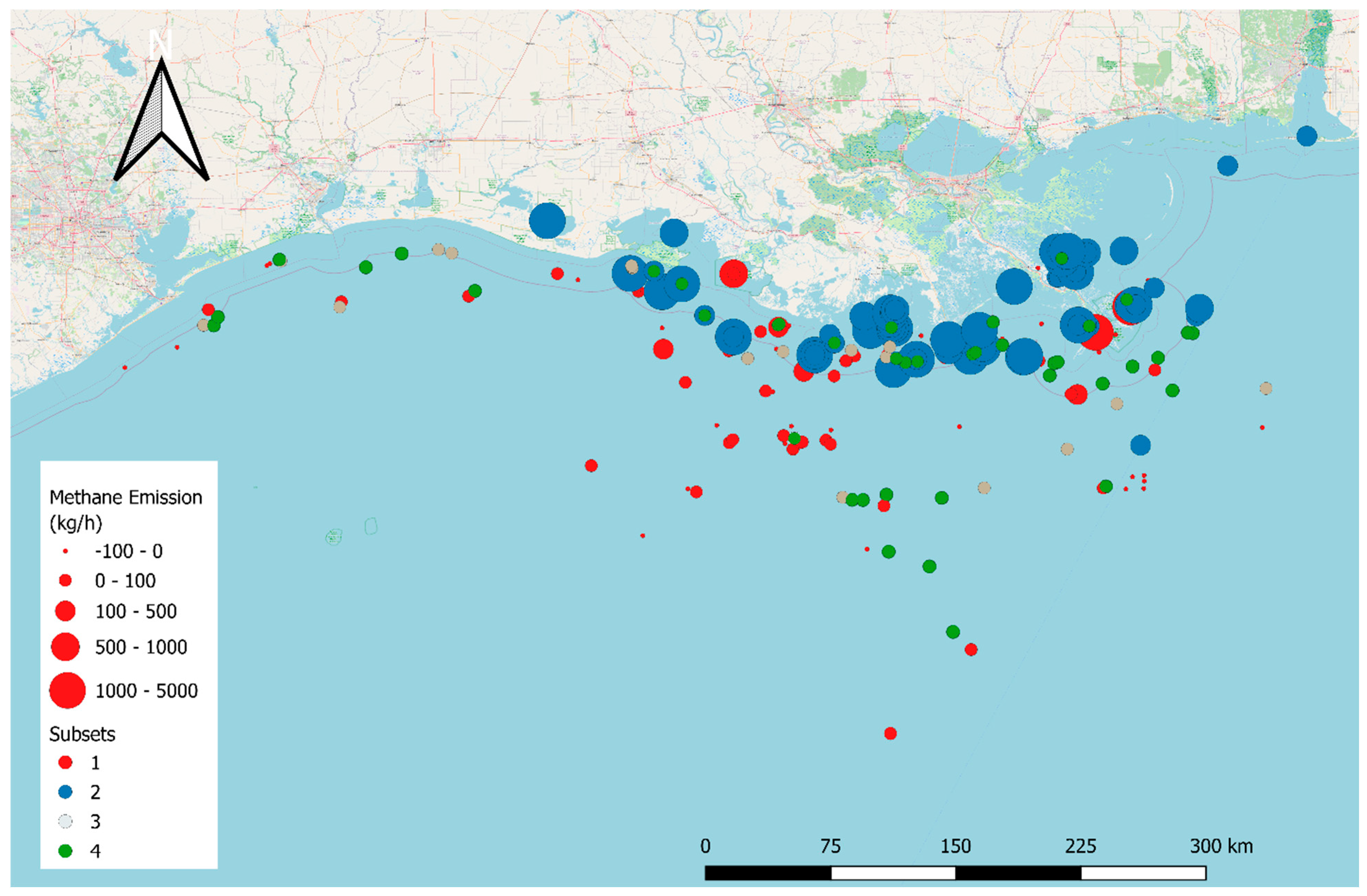
3.3. Potential Measurement Uncertainty and Bias—Case Study Gulf of Mexico

Taking 294 platforms in the Gulf of Mexico measured by downwind methods [7], mass balance [5] and aircraft remote sensing [8], we generated four sub-sets from the combined dataset to investigate if there were geospatial commonalities for measurement data that were either highly uncertain (subset 1), much larger than expected (subset 2), much smaller than expected (subset 3), and those within an expected range given production rates and expected equipment/processes taking place on the facility (subset 4). Specifically, the subsets are defined as 1. likely violated method assumptions; 2. are super emitters following the EPA definition of a facility emitting more than 100 kg CH₄ h⁻¹; 3. Emissions are less than the bottom-up calculated emissions from process and combustion emission of 5.3 kg CH₄ h⁻¹ [77] and 4. are not either subset 1, 2 or 3. Measurements that likely violated method assumptions are those that: 1. were conducted in low wind conditions (<2 m s⁻¹); 2. measurement distances of more than 10 km downwind of the facility; 3. Where the horizontal mass balance transects were made more than 50 m apart vertically; 4. the uncertainties equal to −100%; and 5. there were zero or negative emissions from individual facilities.

Nearly half of the facilities measured (45%) fall into subset 1 and the average emission is 98 kg h⁻¹ as these include very large and very small emissions, (

Table 2. Classification of the 294 platforms measured in the Gulf of Mexico [5,7,8] into subsets that 1. likely violated method assumptions, 2. are super emitters following the EPA definition of a facility emitting more than 100 kg CH₄ h⁻¹, 3. where emissions are less than the bottom-up calculated emissions from process and combustion emission of 5.3 kg CH₄ h⁻¹, and 4. are not either subset 1, 2 or 3.

Classification	Subset 1	Subset 2	Subset 3	Subset 4
Total
Platforms measured	131	102	18	43
Average emission (kg h−1)	98	1012	2	33
Max emission (kg h−1)	4127	4930	5	94
Min emission (kg h−1)	−41	104	0.1	6
Aircraft RS
Platforms Measured	32	95	-	8
Average emission (kg h−1)	277	1060	-	50
Mass balance
Platforms Measured	41	7	-	8
Average emission (kg h−1)	70	360	-	46
Downwind methods
Platforms Measured	58	-	18	27
Average emission (kg h−1)	19	-	2	24

). For the aircraft remote sensing method, 28 observations did not detect an emission, and the other four emissions had an uncertainty greater than ±100%. For the mass balance method, 22 measurements comprised less than 10 transects, 11 measurements were zero emission or less, and 8 measurements were conducted in low wind conditions. For the downwind dispersion, observations were filtered out for those who were not sure which facility was being measured or were more than 10 km from the facility.

Subset 2 includes all very large measurements mostly generated from the aircraft remote sensing approach (95 measurements) with an average emission of 1012 kg CH₄ h⁻¹. We have no methodological reasoning to suggest why subset 2 measurements are not correct, these have been separated to indicate any commonality in spatial distribution. All smaller, non-zero emissions (subset 3) were calculated using the downwind dispersion method. For the 43 measurements in the subset, the average emission is 33 kg h⁻¹ and these are distributed across the three measurement approaches. The largest emissions are generally confined to the near shore and all of these are in either subset 1 or 2 (Figure 1).

4. Discussion

4.1. Review of Methods

This study describes six methods/platforms that could be used to quantify methane emissions from offshore oil and gas production facilities. These include component-level measurements; downwind dispersion approaches; tracer-flux; mass balance; and remote sensing approaches (aircraft and satellite). Each of these has been used to quantify methane emissions from onshore facilities and is now being implemented for offshore quantification.

Downwind dispersion methods have measured 188 offshore facilities globally with an average emission of 32 kg CH₄ h⁻¹ ranging from 0 to 260 kg CH₄ h⁻¹. The advantage of the downwind dispersion method is that it is relatively simple to do (i.e., position a trace methane analyzer downwind of the source). However, this approach makes many assumptions about the size and shape of the plume which may affect quantification in a stratified marine boundary layer and there is the potential for the plume to loft overhead resulting in the non-detection of the plume. During a downwind dispersion campaign in the Gulf of Mexico over half of the facilities were observed to have zero emissions [7]. The downwind dispersion model is the only approach to have been validated by controlled release experiments in a marine environment [52,53].

The mass balance approach has been used to measure emissions from 104 facilities with an average measured emission of 118 kg CH₄ h⁻¹ and maximum and minimum of 1536 and −41 kg CH₄ h⁻¹, respectively. The main advantage of the mass balance approach is that it can be easily visualized, and outputs are visually compelling. The key assumptions associated with the method, as described in Section 2.4, that could affect the quantification are 1. The plume does not move vertically between transect measurements as this could result in double counting the plume (overestimating the emission) or missing the plume altogether (zero emission); and 2. Assuming the plume can be interpolated between horizontal measurements. Upon review of the recently published measurements, it does not appear that either of these assumptions have been completely addressed by any of the studies and the average facility emission estimate is almost a factor of four higher than the downwind dispersion method average emission. The most compelling evidence would be the presentation of the vertical methane enhancement profile downwind of the facility from sea level to the top of the marine boundary layer at relatively small vertical separations (possibly as small as 20 m apart). Most published emissions were derived from mass balance measurements starting at 50 m up to an unreported height with vertical distances as large as 50 m apart, some emission estimates have been generated from as few as three transects.

To our knowledge, there has only been one tracer study conducted on an offshore facility. In our experience, these experiments are very difficult to conduct as they require compressed gas cylinders located relatively close to the emission points in the facilities. This presents a significant health and safety challenge and liability that few operators are willing to take responsibility for. In addition to this, the findings of the tracer flux study found that the emissions were very difficult to replicate with the tracer (i.e., temperature, location, etc.) which resulted in the tracer gas having a very different dispersion behavior than the methane being measured.

The average facility methane emission rates for the remote sensing approaches are 284 kg CH₄ h⁻¹ (max 4930 kg CH₄ h⁻¹ and min 30 kg CH₄ h⁻¹) from 151 facilities and 19,089 kg CH₄ h⁻¹ (max 99,000 kg CH₄ h⁻¹ and min 180 kg CH₄ h⁻¹) from 10 facilities for the aircraft and satellite measurement platforms, respectively. The key assumption for both these methods is that there is a good understanding of the wind speed at the height that the methane has been released. An attempt was made to compare modeled to measured wind speeds at 10 m [8]; however, these measurements were made from a buoy in open water and it is unclear if this is analogous to the wind speed on an offshore production facility where there is a bluff body.

4.2. Possible Causes of Bias or Uncertainty in the Methodologies

All methods of quantification described above have been developed, tuned and evaluated to quantify methane emissions from oil and gas infrastructure. However, these measurements were almost all land-based and there are reservations about deploying these approaches to quantify emissions from offshore production facilities. Some of the uncertainty could be caused by the physical structure within the marine boundary layer and how the wind profile changes when conditions become overcast, which is common, especially in coastal areas.

Stratification, resulting from deep marine boundary layers or solar heating of clouds, could affect methods. The downwind dispersion approach assumes that gas disperses in a uniformly conical shape; however, with the stratification the gas may be entrained in laminar flow or could be reflected at a mid-layer boundary. This could result in either an overestimation of emission, where reflection has not been accounted for, or an underestimation, where the plume has not been observed as it is carried away in an upper stratified layer. The mass balance approach relies on observing the lateral and vertical dispersion of the plume and interpolating between measurement transects. Stratification could affect mass balance methods by:

• In most mass balance surveys, the size and shape of the downwind plume are generated by extrapolating between measurements made at different altitudes. If observations do not extend from 0 m above sea level to the top of the boundary layer, then an extrapolation could be made from the lowest/highest transect height to either sea level or the boundary layer height. A scenario could feasibly exist where a large concentration measurement is observed at the top/bottom transect which is then used to extrapolate a large vertical distance. This would likely result in an overestimation of the vertical size of the plume and overall emission. Care must be taken to ensure that transects bound the top and bottom of the plume.
• If transect measurements are made at relatively sparse vertical sampling heights between sea level and the boundary layer, the plume could be missed and result in zero emissions being observed. This could affect laminar plumes in a stratified MBL as these are likely to be less vertically dispersed than in a well-mixed atmosphere.
• If the winds move the plume vertically on a timescale faster than the time of repeat observations at different heights, plume dynamics could cause you a “double count” if the plume, i.e., the centerline of the plume shifts upwards while the flight is going from low to high, in this way, the calculated emission rate would likely end up with an overestimate.

Remote sensing methods rely on an understanding of wind speed at the emission height. As these data are typically taken from reanalysis data products, it is not currently well understood how accurate the data are. Of note here are the measurements of the aircraft-based remote sensing, where many of the very large emissions were observed at the relatively smaller production coastal facilities in the Gulf of Mexico (Figure 1). In these coastal areas, it is common that near-shore clouds form through either sea breeze convergence or coastal frictional convergence [70], which could result in a decoupling of the marine boundary layer.

To test method accuracy, controlled emissions of methane that simulate actual emission events could be released from a structure representative of a production facility in the open ocean. Experiments could be conducted to test how methods’ emission detection thresholds and quantification uncertainty change with emission type (diffuse, point source, combustion, vented or fugitive), relative location of emission source (e.g., height above ocean, distance from shore, depth of water), and environmental conditions (e.g., stratification, cloud cover, wave height, atmospheric stability). Transparent and comprehensive measurement datasets collected following best-practice protocol could be used to improve the reliability and credibility of emission estimates from offshore facilities. Currently, the suitability of methods used to quantify emissions from offshore facilities is unknown but with a testing program the best practice protocols could be developed, and the uncertainty bounds of quantitation methods would be better understood.

References

1. Statistica. Production of Natural Gas Worldwide in 2022 with a Forecast for 2030 to 2050, by Project Location. Available online: https://www.statista.com/statistics/1365007/natural-gas-production-by-project-location-worldwide/ (accessed on 23 March 2024).
2. EIA. Offshore Production Nearly 30% of Global Crude Oil Output in 2015. Available online: https://www.eia.gov/todayinenergy/detail.php?id=28492 (accessed on 28 December 2021).
3. EIA. Oil and Petroleum Products Explained Offshore Oil and Natural Gas. Available online: https://www.eia.gov/energyexplained/oil-and-petroleum-products/offshore-oil-and-gas-in-depth.php (accessed on 10 June 2020).
4. Biener, K.J.; Gorchov Negron, A.M.; Kort, E.A.; Ayasse, A.K.; Chen, Y.; MacLean, J.-P.; McKeever, J. Temporal Variation and Persistence of Methane Emissions from Shallow Water Oil and Gas Production in the Gulf of Mexico. Environ. Sci. Technol. 2024, 58, 4948–4956. [Google Scholar] [CrossRef] [PubMed]
5. Gorchov Negron, A.M.; Kort, E.A.; Chen, Y.; Brandt, A.R.; Smith, M.L.; Plant, G.; Ayasse, A.K.; Schwietzke, S.; Zavala-Araiza, D.; Hausman, C.; et al. Excess Methane Emissions from Shallow Water Platforms Elevate the Carbon Intensity of US Gulf of Mexico Oil and Gas Production. Proc. Natl. Acad. Sci. USA 2023, 120, e2215275120. [Google Scholar] [CrossRef] [PubMed]
6. Gorchov Negron, A.M.; Kort, E.A.; Conley, S.A.; Smith, M.L. Airborne Assessment of Methane Emissions from Offshore Platforms in the U.S. Gulf of Mexico. Environ. Sci. Technol. 2020, 54, 5112–5120. [Google Scholar] [CrossRef]
7. Ayasse, A.K.; Thorpe, A.K.; Cusworth, D.H.; Kort, E.A.; Negron, A.G.; Heckler, J.; Asner, G.; Duren, R.M. Methane Remote Sensing and Emission Quantification of Offshore Shallow Water Oil and Gas Platforms in the Gulf of Mexico. Environ. Res. Lett. 2022, 17, 084039. [Google Scholar] [CrossRef]
8. Yacovitch, T.I.; Daube, C.; Herndon, S.C. Methane Emissions from Offshore Oil and Gas Platforms in the Gulf of Mexico. Environ. Sci. Technol. 2020, 54, 3530–3538. [Google Scholar] [CrossRef]
9. Speight, J.G. Handbook of Offshore Oil and Gas Operations, 1st ed.; Elsevier Gulf Professional Publishing: Amsterdam, The Netherlands; Boston, MA, USA; Waltham, MA, USA, 2015; ISBN 978-1-85617-558-6. [Google Scholar]
10. BSEE. Bureau of Safety and Environmental Enforcement (BSEE) Data Center. Available online: https://www.data.bsee.gov/Main/Default.aspx (accessed on 23 March 2024).
11. Barkley, Z.; Davis, K.; Miles, N.; Richardson, S.; Deng, A.; Hmiel, B.; Lyon, D.; Lauvaux, T. Quantification of Oil and Gas Methane Emissions in the Delaware and Marcellus Basins Using a Network of Continuous Tower-Based Measurements. Atmos. Chem. Phys. 2023, 23, 6127–6144. [Google Scholar] [CrossRef]
12. Alvarez, R.A.; Zavala-Araiza, D.; Lyon, D.R.; Allen, D.T.; Barkley, Z.R.; Brandt, A.R.; Davis, K.J.; Herndon, S.C.; Jacob, D.J.; Karion, A.; et al. Assessment of Methane Emissions from the U.S. Oil and Gas Supply Chain. Science 2018, 361, eaar7204. [Google Scholar] [CrossRef]
13. Ravikumar, A.P.; Wang, J.; Brandt, A.R. Are Optical Gas Imaging Technologies Effective For Methane Leak Detection? Environ. Sci. Technol. 2017, 51, 718–724. [Google Scholar] [CrossRef]
14. Rutherford, J.S.; Sherwin, E.D.; Ravikumar, A.P.; Heath, G.A.; Englander, J.; Cooley, D.; Lyon, D.; Omara, M.; Langfitt, Q.; Brandt, A.R. Closing the Methane Gap in US Oil and Natural Gas Production Emissions Inventories. Nat. Commun. 2021, 12, 4715. [Google Scholar] [CrossRef]
15. Omara, M.; Sullivan, M.R.; Li, X.; Subramanian, R.; Robinson, A.L.; Presto, A.A. Methane Emissions from Conventional and Unconventional Natural Gas Production Sites in the Marcellus Shale Basin. Environ. Sci. Technol. 2016, 50, 2099–2107. [Google Scholar] [CrossRef]
16. Robertson, A.M.; Edie, R.; Field, R.A.; Lyon, D.; McVay, R.; Omara, M.; Zavala-Araiza, D.; Murphy, S.M. New Mexico Permian Basin Measured Well Pad Methane Emissions Are a Factor of 5–9 Times Higher Than U.S. EPA Estimates. Environ. Sci. Technol. 2020, 54, 13926–13934. [Google Scholar] [CrossRef]
17. Sherwin, E.D.; Rutherford, J.S.; Chen, Y.; Aminfard, S.; Kort, E.A.; Jackson, R.B.; Brandt, A.R. Single-Blind Validation of Space-Based Point-Source Detection and Quantification of Onshore Methane Emissions. Sci. Rep. 2023, 13, 3836. [Google Scholar] [CrossRef]
18. IPCC. Climate Change 2022: Impacts, Adaptation and Vulnerability. Contribution of Working Group II to the Sixth Assessment Report of the Intergovernmental Panel on Climate Change; Pörtner, H.-O., Roberts, D.C., Tignor, M., Poloczanska, E.S., Mintenbeck, K., Alegría, A., Craig, M., Langsdorf, S., Löschke, S., Möller, V., et al., Eds.; Cambridge University Press: Cambridge, UK; New York, NY, USA, 2022; ISBN 978-1-009-32584-4. [Google Scholar]
19. Stocker, T. (Ed.) Climate Change 2013: The Physical Science Basis: Working Group I Contribution to the Fifth Assessment Report of the Intergovernmental Panel on Climate Change; Cambridge University Press: Cambridge, UK, 2014; ISBN 978-1-107-41532-4. [Google Scholar]
20. Nisbet, E.G.; Fisher, R.E.; Lowry, D.; France, J.L.; Allen, G.; Bakkaloglu, S.; Broderick, T.J.; Cain, M.; Coleman, M.; Fernandez, J.; et al. Methane Mitigation: Methods to Reduce Emissions, on the Path to the Paris Agreement. Rev. Geophys. 2020, 58, e2019RG000675. [Google Scholar] [CrossRef]
21. Nisbet, E.G.; Manning, M.R.; Dlugokencky, E.J.; Fisher, R.E.; Lowry, D.; Michel, S.E.; Myhre, C.L.; Platt, S.M.; Allen, G.; Bousquet, P.; et al. Very Strong Atmospheric Methane Growth in the 4 Years 2014–2017: Implications for the Paris Agreement. Global Biogeochem. Cycles 2019, 33, 318–342. [Google Scholar] [CrossRef]
22. Vaughn, T.L.; Bell, C.S.; Yacovitch, T.I.; Roscioli, J.R.; Herndon, S.C.; Conley, S.; Schwietzke, S.; Heath, G.A.; Pétron, G.; Zimmerle, D. Comparing Facility-Level Methane Emission Rate Estimates at Natural Gas Gathering and Boosting Stations. Elem. Sci. Anthr. 2017, 5, 71. [Google Scholar] [CrossRef]
23. Bell, C.S.; Vaughn, T.L.; Zimmerle, D.; Herndon, S.C.; Yacovitch, T.I.; Heath, G.A.; Pétron, G.; Edie, R.; Field, R.A.; Murphy, S.M.; et al. Comparison of Methane Emission Estimates from Multiple Measurement Techniques at Natural Gas Production Pads. Elem. Sci. Anthr. 2017, 5, 79. [Google Scholar] [CrossRef]
24. Riddick, S.N.; Mbua, M.; Santos, A.; Emerson, E.W.; Cheptonui, F.; Houlihan, C.; Hodshire, A.L.; Anand, A.; Hartzell, W.; Zimmerle, D.J. Methane Emissions from Abandoned Oil and Gas Wells in Colorado. Sci. Total Environ. 2024, 922, 170990. [Google Scholar] [CrossRef]
25. Caulton, D.R.; Li, Q.; Bou-Zeid, E.; Fitts, J.P.; Golston, L.M.; Pan, D.; Lu, J.; Lane, H.M.; Buchholz, B.; Guo, X.; et al. Quantifying Uncertainties from Mobile-Laboratory-Derived Emissions of Well Pads Using Inverse Gaussian Methods. Atmos. Chem. Phys. 2018, 18, 15145–15168. [Google Scholar] [CrossRef]
26. Edie, R.; Robertson, A.M.; Field, R.A.; Soltis, J.; Snare, D.A.; Zimmerle, D.; Bell, C.S.; Vaughn, T.L.; Murphy, S.M. Constraining the Accuracy of Flux Estimates Using OTM 33A. Atmos. Meas. Tech. 2020, 13, 341–353. [Google Scholar] [CrossRef]
27. Riddick, S.N.; Cheptonui, F.; Yuan, K.; Mbua, M.; Day, R.; Vaughn, T.L.; Duggan, A.; Bennett, K.E.; Zimmerle, D.J. Estimating Regional Methane Emission Factors from Energy and Agricultural Sector Sources Using a Portable Measurement System: Case Study of the Denver–Julesburg Basin. Sensors 2022, 22, 7410. [Google Scholar] [CrossRef]
28. Lamb, B.K.; McManus, J.B.; Shorter, J.H.; Kolb, C.E.; Mosher, B.; Harriss, R.C.; Allwine, E.; Blaha, D.; Howard, T.; Guenther, A.; et al. Development of Atmospheric Tracer Methods To Measure Methane Emissions from Natural Gas Facilities and Urban Areas. Environ. Sci. Technol. 1995, 29, 1468–1479. [Google Scholar] [CrossRef] [PubMed]
29. Conley, S.A.; Faloona, I.C.; Lenschow, D.H.; Karion, A.; Sweeney, C. A Low-Cost System for Measuring Horizontal Winds from Single-Engine Aircraft. J. Atmos. Ocean. Technol. 2014, 31, 1312–1320. [Google Scholar] [CrossRef]
30. Cusworth, D.H.; Jacob, D.J.; Varon, D.J.; Chan Miller, C.; Liu, X.; Chance, K.; Thorpe, A.K.; Duren, R.M.; Miller, C.E.; Thompson, D.R.; et al. Potential of Next-Generation Imaging Spectrometers to Detect and Quantify Methane Point Sources from Space. Atmos. Meas. Tech. 2019, 12, 5655–5668. [Google Scholar] [CrossRef]
31. Duren, R.M.; Thorpe, A.K.; Foster, K.T.; Rafiq, T.; Hopkins, F.M.; Yadav, V.; Bue, B.D.; Thompson, D.R.; Conley, S.; Colombi, N.K.; et al. California’s Methane Super-Emitters. Nature 2019, 575, 180–184. [Google Scholar] [CrossRef] [PubMed]
32. Kunkel, W.M.; Carre-Burritt, A.E.; Aivazian, G.S.; Snow, N.C.; Harris, J.T.; Mueller, T.S.; Roos, P.A.; Thorpe, M.J. Extension of Methane Emission Rate Distribution for Permian Basin Oil and Gas Production Infrastructure by Aerial LiDAR. Environ. Sci. Technol. 2023, 57, 12234–12241. [Google Scholar] [CrossRef]
33. Ayasse, A.K.; Dennison, P.E.; Foote, M.; Thorpe, A.K.; Joshi, S.; Green, R.O.; Duren, R.M.; Thompson, D.R.; Roberts, D.A. Methane Mapping with Future Satellite Imaging Spectrometers. Remote Sens. 2019, 11, 3054. [Google Scholar] [CrossRef]
34. Jervis, D.; McKeever, J.; Durak, B.O.A.; Sloan, J.J.; Gains, D.; Varon, D.J.; Ramier, A.; Strupler, M.; Tarrant, E. The GHGSat-D Imaging Spectrometer. Atmos. Meas. Tech. 2021, 14, 2127–2140. [Google Scholar] [CrossRef]
35. MacLean, J.-P.W.; Girard, M.; Jervis, D.; Marshall, D.; McKeever, J.; Ramier, A.; Strupler, M.; Tarrant, E.; Young, D. Offshore Methane Detection and Quantification from Space Using Sun Glint Measurements with the GHGSat Constellation. Atmos. Meas. Tech. 2024, 17, 863–874. [Google Scholar] [CrossRef]
36. Irakulis-Loitxate, I.; Gorroño, J.; Zavala-Araiza, D.; Guanter, L. Satellites Detect a Methane Ultra-Emission Event from an Offshore Platform in the Gulf of Mexico. Environ. Sci. Technol. Lett. 2022, 9, 520–525. [Google Scholar] [CrossRef]
37. Valverde, A.; Irakulis-Loitxate, I.; Roger, J.; Gorroño, J.; Guanter, L. Satellite Characterization of Methane Point Sources by Offshore Oil and Gas PlatForms. Environ. Sci. Proc. 2023, 28, 22. [Google Scholar]
38. Stamnes, K. Methane Detection from Space: Use of Sunglint. Opt. Eng. 2006, 45, 016202. [Google Scholar] [CrossRef]
39. Seinfeld, J.H.; Pandis, S.N. Atmospheric Chemistry and Physics: From Air Pollution to Climate Change, 3rd ed.; John Wiley & Sons, Inc.: Hoboken, NJ, USA, 2016; ISBN 978-1-118-94740-1. [Google Scholar]
40. Garratt, J. Review: The Atmospheric Boundary Layer. Earth-Sci. Rev. 1994, 37, 89–134. [Google Scholar] [CrossRef]
41. Garratt, J.R. The Atmospheric Boundary Layer; Cambridge Atmospheric and Space Science Series; Cambridge University Press: Cambridge, UK, 1994; ISBN 978-0-521-46745-2. [Google Scholar]
42. Albrecht, B.A.; Jensen, M.P.; Syrett, W.J. Marine Boundary Layer Structure and Fractional Cloudiness. J. Geophys. Res. 1995, 100, 14209–14222. [Google Scholar] [CrossRef]
43. Galewsky, J.; Jensen, M.P.; Delp, J. Marine Boundary Layer Decoupling and the Stable Isotopic Composition of Water Vapor. JGR Atmos. 2022, 127, e2021JD035470. [Google Scholar] [CrossRef]
44. BOEM US Bureau of Ocean Energy Management (BOEM). Outer Continental Shelf Air Quality System (OCS AQS): Year 2021 Emissions Inventory. Available online: https://www.boem.gov/Gulfwide-Offshore-Activity-Data-System-GOADS/ (accessed on 23 March 2024).
45. Heath SEMTECH® HI-FLOW 2. Available online: https://heathus.com/product/semtech-hi-flow-2/ (accessed on 17 May 2025).
46. Vaughn, T.L.; Ross, C.; Zimmerle, D.J.; Bennett, K.E.; Harrison, M.; Wilson, A.; Johnson, C. Open-Source High Flow Sampler for Natural Gas Leak Quantification. Available online: https://mountainscholar.org/items/ad820fd7-ee72-4277-afbd-0eb96231d95f (accessed on 17 May 2025).
47. Riddick, S.N.; Ancona, R.; Mbua, M.; Bell, C.S.; Duggan, A.; Vaughn, T.L.; Bennett, K.; Zimmerle, D.J. A Quantitative Comparison of Methods Used to Measure Smaller Methane Emissions Typically Observed from Superannuated Oil and Gas Infrastructure. Atmos. Meas. Tech. 2022, 15, 6285–6296. [Google Scholar] [CrossRef]
48. Pasquill, F. Atmospheric diffusion. By F. Pasquill. London (Van Nostrand Co.), 1962. Pp. Xii, 297; 60s. Q. J. R. Meteorol. Soc. 1962, 88, 202–203. [Google Scholar] [CrossRef]
49. Pasquill, F. Limitations and Prospects in the Estimation of Dispersion of Pollution on a Regional Scale. In Advances in Geophysics; Elsevier: Amsterdam, The Netherlands, 1975; Volume 18, pp. 1–13. ISBN 978-0-12-018848-2. [Google Scholar]
50. Pasquill, F.; Smith, F.B. Atmospheric Diffusion, 3rd ed.; Ellis Horwood, (John Wiley & Sons): Chichester, UK, 1983; Volume 110. [Google Scholar]
51. US EPA Industrial Source Complex (ISC3) Dispersion Model; User’s Guide. EPA 454/B 95 003a (Vol. I) and EPA 454/B 95 003b (Vol. II); U.S. Environmental Protection Agency: Research Triangle Park, NC, USA, 1995.
52. Blackall, T.D.; Wilson, L.J.; Bull, J.; Theobald, M.R.; Bacon, P.J.; Hamer, K.C.; Wanless, S.; Sutton, M.A. Temporal Variation in Atmospheric Ammonia Concentrations Above Seabird Colonies. Atmos. Environ. 2008, 42, 6942–6950. [Google Scholar] [CrossRef]
53. Blackall, T.D.; Wilson, L.J.; Theobald, M.R.; Milford, C.; Nemitz, E.; Bull, J.; Bacon, P.J.; Hamer, K.C.; Wanless, S.; Sutton, M.A. Ammonia Emissions from Seabird Colonies. Geophys. Res. Lett. 2007, 34. [Google Scholar] [CrossRef]
54. Denmead, O.T. Approaches to Measuring Fluxes of Methane and Nitrous Oxide Between Landscapes and the Atmosphere. Plant Soil 2008, 309, 5–24. [Google Scholar] [CrossRef]
55. Subramanian, R.; Williams, L.L.; Vaughn, T.L.; Zimmerle, D.; Roscioli, J.R.; Herndon, S.C.; Yacovitch, T.I.; Floerchinger, C.; Tkacik, D.S.; Mitchell, A.L.; et al. Methane Emissions from Natural Gas Compressor Stations in the Transmission and Storage Sector: Measurements and Comparisons with the EPA Greenhouse Gas Reporting Program Protocol. Environ. Sci. Technol. 2015, 49, 3252–3261. [Google Scholar] [CrossRef]
56. Allen, D.T. Emissions from Oil and Gas Operations in the United States and Their Air Quality Implications. J. Air Waste Manag. Assoc. 2016, 66, 549–575. [Google Scholar] [CrossRef] [PubMed]
57. Fredenslund, A.M.; Rees-White, T.C.; Beaven, R.P.; Delre, A.; Finlayson, A.; Helmore, J.; Allen, G.; Scheutz, C. Validation and Error Assessment of the Mobile Tracer Gas Dispersion Method for Measurement of Fugitive Emissions from Area Sources. Waste Manag. 2019, 83, 68–78. [Google Scholar] [CrossRef] [PubMed]
58. Conley, S.; Faloona, I.; Mehrotra, S.; Suard, M.; Lenschow, D.H.; Sweeney, C.; Herndon, S.; Schwietzke, S.; Pétron, G.; Pifer, J.; et al. Application of Gauss’s Theorem to Quantify Localized Surface Emissions from Airborne Measurements of Wind and Trace Gases. Atmos. Meas. Tech. 2017, 10, 3345–3358. [Google Scholar] [CrossRef]
59. Cooper, J.; Dubey, L.; Hawkes, A. Methane Detection and Quantification in the Upstream Oil and Gas Sector: The Role of Satellites in Emissions Detection, Reconciling and Reporting. Environ. Sci. Atmos. 2022, 2, 9–23. [Google Scholar] [CrossRef]
60. Schneising, O.; Buchwitz, M.; Reuter, M.; Bovensmann, H.; Burrows, J.P.; Borsdorff, T.; Deutscher, N.M.; Feist, D.G.; Griffith, D.W.T.; Hase, F.; et al. A Scientific Algorithm to Simultaneously Retrieve Carbon Monoxide and Methane from TROPOMI Onboard Sentinel-5 Precursor. Atmos. Meas. Tech. 2019, 12, 6771–6802. [Google Scholar] [CrossRef]
61. Veefkind, J.P.; Aben, I.; McMullan, K.; Förster, H.; De Vries, J.; Otter, G.; Claas, J.; Eskes, H.J.; De Haan, J.F.; Kleipool, Q.; et al. TROPOMI on the ESA Sentinel-5 Precursor: A GMES Mission for Global Observations of the Atmospheric Composition for Climate, Air Quality and Ozone Layer Applications. Remote Sens. Environ. 2012, 120, 70–83. [Google Scholar] [CrossRef]
62. Riddick, S.N.; Mauzerall, D.L.; Celia, M.; Harris, N.R.P.; Allen, G.; Pitt, J.; Staunton-Sykes, J.; Forster, G.L.; Kang, M.; Lowry, D.; et al. Methane Emissions from Oil and Gas Platforms in the North Sea. Atmos. Chem. Phys. 2019, 19, 9787–9796. [Google Scholar] [CrossRef]
63. Nara, H.; Tanimoto, H.; Tohjima, Y.; Mukai, H.; Nojiri, Y.; Machida, T. Emissions of Methane from Offshore Oil and Gas Platforms in Southeast Asia. Sci. Rep. 2015, 4, 6503. [Google Scholar] [CrossRef]
64. Zang, K.; Zhang, G.; Wang, J. Methane Emissions from Oil and Gas Platforms in the Bohai Sea, China. Environ. Pollut. 2020, 263, 114486. [Google Scholar] [CrossRef]
65. Hensen, A.; Velzeboer, I.; Frumau, K.F.A.; van den Bulk, W.C.M.; van Dinter, D. Methane Emission Measurements of Offshore Oil and Gas Platforms; TNO: Petten, The Netherlands, 2019; p. 94. [Google Scholar]
66. Khaleghi, A.; MacKay, K.; Darlington, A.; James, L.A.; Risk, D. Methane Emission Rate Estimates of Offshore Oil Platforms in Newfoundland and Labrador, Canada. Elem. Sci. Anthr. 2024, 12, 00025. [Google Scholar] [CrossRef]
67. Fiehn, A.; Eckl, M.; Bräuer, T.; Pühl, M.; Dapurkar, N.; Gottschaldt, K.-D.; Aufmhoff, H.; Eirenschmalz, L.; Neumann, G.; Sakellariou, F.; et al. Aircraft-Based Mass Balance Estimate of Methane Emissions from the Offshore Oil Industry in Angola. In Proceedings of the EGU General Assembly 2024, Vienna, Austria, 14–19 April 2024. [Google Scholar]
68. Pühl, M.; Roiger, A.; Fiehn, A.; Gorchov Negron, A.M.; Kort, E.A.; Schwietzke, S.; Pisso, I.; Foulds, A.; Lee, J.; France, J.L.; et al. Aircraft-Based Mass Balance Estimate of Methane Emissions from Offshore Gas Facilities in the Southern North Sea. Atmos. Chem. Phys. 2024, 24, 1005–1024. [Google Scholar] [CrossRef]
69. Zavala-Araiza, D.; Omara, M.; Gautam, R.; Smith, M.L.; Pandey, S.; Aben, I.; Almanza-Veloz, V.; Conley, S.; Houweling, S.; Kort, E.A.; et al. A Tale of Two Regions: Methane Emissions from Oil and Gas Production in Offshore/Onshore Mexico. Environ. Res. Lett. 2021, 16, 024019. [Google Scholar] [CrossRef]
70. Jiménez, M.A.; Simó, G.; Wrenger, B.; Telisman-Prtenjak, M.; Guijarro, J.A.; Cuxart, J. Morning Transition Case Between the Land and the Sea Breeze Regimes. Atmos. Res. 2016, 172–173, 95–108. [Google Scholar] [CrossRef]
71. Foulds, A.; Allen, G.; Shaw, J.T.; Bateson, P.; Barker, P.A.; Huang, L.; Pitt, J.R.; Lee, J.D.; Wilde, S.E.; Dominutti, P.; et al. Quantification and Assessment of Methane Emissions from Offshore Oil and Gas Facilities on the Norwegian Continental Shelf. Atmos. Chem. Phys. 2022, 22, 4303–4322. [Google Scholar] [CrossRef]
72. Lee, J.D.; Mobbs, S.D.; Wellpott, A.; Allen, G.; Bauguitte, S.J.-B.; Burton, R.R.; Camilli, R.; Coe, H.; Fisher, R.E.; France, J.L.; et al. Flow Rate and Source Reservoir Identification from Airborne Chemical Sampling of the Uncontrolled Elgin Platform Gas Release. Atmos. Meas. Tech. 2018, 11, 1725–1739. [Google Scholar] [CrossRef]
73. Cain, M.; Warwick, N.J.; Fisher, R.E.; Lowry, D.; Lanoisellé, M.; Nisbet, E.G.; France, J.; Pitt, J.; O’Shea, S.; Bower, K.N.; et al. A Cautionary Tale: A Study of a Methane Enhancement over the North Sea. J. Geophys. Res. Atmos. 2017, 122, 7630–7645. [Google Scholar] [CrossRef]
74. Purvis, R.; Lee, J.; Moore, T.; Burton, R.; Hopkins, J.; Lewis, A.; Mobbs, S.; Young, S. Emissions of Methane and Volatile Organic Compounds from Offshore Oil Loading Using Shuttle Tankers. In Proceedings of the EGU General Assembly 2024, Vienna, Austria, 14–19 April 2024. [Google Scholar]
75. France, J.L.; Bateson, P.; Dominutti, P.; Allen, G.; Andrews, S.; Bauguitte, S.; Coleman, M.; Lachlan-Cope, T.; Fisher, R.E.; Huang, L.; et al. Facility Level Measurement of Offshore Oil and Gas Installations from a Medium-Sized Airborne Platform: Method Development for Quantification and Source Identification of Methane Emissions. Atmos. Meas. Tech. 2021, 14, 71–88. [Google Scholar] [CrossRef]
76. Dahan, B.; Machuca, V.; Castillo, R.; Hess, M. Gulf of Mexico Health & Air Quality II Mapping Methane Emission Plumes Using Sunglint-Configured Imagery for Monitoring Offshore Oil & Gas Activity. NASA DEVELOP National Program California—JPL. Fall 2022. Available online: https://ntrs.nasa.gov/api/citations/20230001674/downloads/20230001674.pdf (accessed on 5 May 2025).
77. Riddick, S.N.; Mauzerall, D.L. Likely Substantial Underestimation of Reported Methane Emissions from United Kingdom Upstream Oil and Gas Activities. Energy Environ. Sci. 2023, 16, 295–304. [Google Scholar] [CrossRef]
Figure 1. Distribution and relative sizes of the 294 platforms measured in the Gulf of Mexico [5,7,8]. Measurements are split into subsets of those 1. likely violated method assumptions, 2. are super emitters following the EPA definition of a facility emitting more than 100 kg CH4 h−1, 3. Emissions are less than the bottom-up calculated emissions from process and combustion emission of 5.3 kg CH4 h−1 and 4. are not either subset 1, 2 or 3.
Atmosphere 16 00626 g001