A Method for Building the Grid-Based Atmospheric Weighted Mean Temperature Model Considering the Hourly NSTLR

Abstract

The weighted mean temperature (T_m) is a critical parameter for converting zenith wet delay (ZWD) to precipitable water vapor (PWV) in Global Navigation Satellite System (GNSS) meteorology. Unlike conventional approaches, this study develops a novel high-precision atmospheric Tm grid model with enhanced spatiotemporal resolution through the incorporation of hourly near-surface temperature lapse rates (NSTLR). The core methodology encompasses two principal components: regional estimation of hourly NSTLR variations and establishment of a corresponding Tm grid model. Validation was conducted using ERA5 reanalysis datasets and in situ measurements from 109 meteorological stations across Shandong Province and Sichuan Province, China. Compared with no environmental lapse rate (ELR) correction and constant ELR correction, the accuracy of the constructed Tm grid model improved by 31.59% and 11.51%, respectively. Notably, in high-altitude areas, the improvements were even more substantial, reaching 58.65% and 21.28%, respectively. Therefore, the Tm model constructed in this study has significant practical significance for building ground-based meteorological observation systems, especially for regions with significant terrain variations.

1. Introduction

The weighted mean temperature ($T_m$) is a critical parameter in determining the conversion factor for precipitable water vapor (PWV) in Global Navigation Satellite System (GNSS) meteorology [1]. Although $T_m$ can be obtained by integrating radiosonde observations or atmospheric reanalysis datasets, the inherent latency in data publication impedes real-time or near-real-time $T_m$ estimation. To improve computational efficiency and facilitate operational meteorological applications, empirical models based on surface meteorological measurements and non-meteorological parameters have been widely developed for GNSS-based PWV retrieval.

A seminal study by Bevis et al. [2] established a foundational model using measured meteorological data by analyzing the relationship between surface temperature ($T_s$) and $T_m$ using 8718 radiosonde profiles across North America. Their results demonstrated a robust linear correlation, formulated as $T_m=a+b\cdot T_s$. Subsequent research efforts [3,4,5,6] have expanded upon this work, deriving region-specific linear regression coefficients through analogous analyses in diverse geographical regions using various types of surface meteorological observations. These localized models improve the accuracy and applicability of $T_m$ estimation for GNSS PWV inversion.

Non-meteorological parameter models, which estimate $T_m$ using station location and temporal information, are typically classified as empirical $T_m$ models. Building upon the Global Pressure and Temperature (GPT) model, Yao et al. developed the Global Wet Mean Temperature (GWMT) model based on data from 135 global radiosonde stations. Subsequent improvements in modeling techniques and source data have led to the development of enhanced models, including GTm-II, GTm-III, GWMT-IV, GTM-X, and GWMT-D [7]. Huang et al. introduced the GGTm model, incorporating a sliding window algorithm to account for latitudinal and altitudinal variations [8]. Meanwhile, Sun et al. proposed the GTrop model, which integrates linear trends, annual and semi-annual variations, and spatial dependencies [9]. Additionally, widely used empirical tropospheric models such as GPT3 and UNB3m also provide $T_m$ estimates [10,11]. Although these empirical models are practical, they often struggle to accurately represent localized atmospheric complexity. Compared to regression models derived from surface temperature data, their accuracy is usually lower [6].

In recent years, ground-based meteorological observations have emerged as a convenient and efficient data source for calculating $T_m$, owing to their controllable measurements, real-time availability, dense station distribution, and high spatiotemporal resolution. These advantages substantially improve the accuracy of precipitable water vapor retrieval in both post-processing and real-time applications. However, a considerable number of GNSS stations were not originally established for meteorological applications and thus lack co-located meteorological sensors [2]. Consequently, obtaining reliable and consistent $T_m$ estimates at GNSS sites remains a critical challenge in PWV retrieval. A conventional solution involves spatially interpolating temperature data from nearby meteorological stations to GNSS locations and applying empirical $T_m$ models [12]. However, this approach faces two primary challenges.

First, the vertical variation in temperature during interpolation must be addressed using appropriate temperature lapse rates. While the tropospheric environmental lapse rate (ELR) averages 0.65 °C/100 m in the free atmosphere, substantial deviations from this standard rate often occur due to atmospheric conditions [13,14]. In contrast to the ELR, which describes temperature changes across the boundary layer and free atmosphere, the near-surface temperature lapse rate (NSTLR) characterizes thermal variations within the surface layer [15,16,17,18]. Studies have demonstrated that employing the NSTLR instead of the ELR can significantly improve the accuracy of temperature interpolation [2]. However, the NSTLR itself exhibits spatiotemporal variability influenced by geographic location, topography, and thermal dynamics [19]. A high-temporal-resolution NSTLR is particularly crucial for capturing elevation-dependent temperature variations. Ensuring precise and temporally resolved $T_m$ estimates at GNSS stations, especially in complex high-altitude terrains [17].

The second challenge lies in accessing measured temperature data, as most meteorological station observations require authorization (http://data.cma.cn). Furthermore, general users often encounter difficulties in obtaining precise station location details and face technical barriers related to unidirectional data transmission and large-volume data processing. These constraints hinder real-time GNSS PWV estimation. To overcome these limitations, it is essential to develop a high-precision regional grid model for $T_m$ interpolation, incorporating discrete meteorological station temperatures and the NSTLR. Such a model would allow the dissemination of gridded temperature data and corresponding coordinates without disclosing the exact locations of the source stations, thereby facilitating broader accessibility while maintaining data integrity and confidentiality.

Based on the above analysis, it can be concluded that $T_m$ models have made significant progress in terms of construction methods and data sources. These models combine spatially variable transition rates to better explain terrain effects. For instance, the GGTm model [8] employs a sliding window algorithm to capture latitudinal and altitudinal variations, while the GTrop model [9] integrates linear trends and periodic oscillations. Regional studies have further highlighted the importance of the NSTLR over standard environmental lapse rates for temperature interpolation in complex terrain [17,18]. However, many of these approaches still rely on fixed seasonal or daily average lapse rates. This may not fully capture the pronounced diurnal variability of the NSTLR, especially in regions with significant solar heating and complex topography. This temporal oversimplification can limit the accuracy of high-resolution $T_m$ estimation required for real-time GNSS meteorology applications.

The primary objective of this investigation is to establish an improved $T_m$ modeling approach that systematically accounts for temporal variations in NSTLR at hourly intervals. The study encompasses three main components: regional characterization of hourly NSTLR patterns, implementation of an advanced $T_m$ interpolation scheme, and rigorous accuracy assessment through diverse validation methodologies.

2. Materials and Methods

2.1. Study Area

The study area encompasses Shandong Province, located in eastern China, which exhibits distinct topographic variations across the region. The central portion is dominated by uplifted mountainous terrain, whereas the eastern and southern sections are characterized by gently undulating hills. In contrast, the northern and northwestern regions comprise flat alluvial plains. The highest elevation within the study area is at Mount Tai (indicated by the red dot in Figure 1), with a peak altitude of approximately 1545 m above sea level. A high-precision meteorological monitoring station has been installed at this summit. Conversely, the lowest elevations are found in the plains, averaging around 34.9 m. To construct the grid-based model, observational data from 109 officially authorized meteorological stations across the region were utilized. These stations, illustrated in Figure 1, provided hourly temperature measurements spanning the period from January 2021 to December 2022 (http://data.cma.cn). Among all meteorological stations, 84 stations were used to construct the $T_m$ grid model, and 25 stations were used for validation. The 25 validation stations were selected to include 8 stations in each of the elevation ranges of 0~100 m, 100~180 m, and 180~350 m. The other testing station is the highest point in the research area (with an elevation of 1536.5 m).

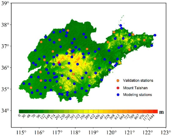
Figure 1. Distribution of topography and meteorological stations in Shandong Province in eastern China.

2.2. Accurate Estimation of Hourly NSTLR

The troposphere, as one of the most important components of the Earth’s space environment, contains almost all of the atmospheric water vapor in the entire Earth’s atmosphere. GNSS electromagnetic wave signals are affected by atmospheric effects when passing through the troposphere, resulting in refraction and bending of satellite signals, known as tropospheric delay. Its projection in the zenith direction of the station is called zenith tropospheric delay (ZTD). ZTD includes two parts: zenith hydrostatic delay (ZHD) and zenith wet delay (ZWD). Although ZWD accounts for a relatively small proportion in ZTD, it is a key parameter for PWV inversion. Thus, the PWV at a GNSS station can be derived through the transformation of the ZWD using a dimensionless conversion factor $K$, as expressed in Equations (1) and (2) [2]:

$$\mathrm{PWV}=K\cdot \mathrm{ZWD}$$

(1)

$$K={\displaystyle \frac{{10}^6}{{\rho }_w{R}_w(\frac{k_3}{T_m}+k_2^{\prime })}}$$

(2)

Here, $k_2^{\prime }=17\pm 10\mathrm{K}/\mathrm{hPa}$ and $k_3=3.776\pm 0.004\times {10}^5{\mathrm{K}}^2/\mathrm{hPa}$ denote the empirically derived atmospheric refractivity constants. The term $R_w=461.51\mathrm{J}/(\mathrm{K}\cdot \mathrm{kg})$ represents the specific gas constant for water vapor, while ${\rho }_w=1000\mathrm{kg}\cdot {\mathrm{m}}^{-3}$ is the standard density of liquid water. The variable $T_m$ corresponds to the weighted mean temperature, expressed in Kelvin ($K$). ZWD can be obtained through GNSS precise point positioning or differential positioning.

According to Formula (2), accurate determination of the $T_m$ constitutes a critical factor in enhancing PWV estimation precision. Utilize the inherent advantages of meteorological station networks, including operational controllability, robust real-time data collection, dense spatial coverage, and high spatiotemporal resolution. This study developed a grid model that maintains high accuracy and practical feasibility while maintaining station confidentiality. The fundamental challenge in this modeling approach is to establish the precise functional relationship between surface temperature ($T_s$) and $T_m$. Building upon the latitude-dependent linear regression framework established by Yao et al. [19], this relationship can be mathematically expressed as

$$T_m=a+b\cdot T_s$$

(3)

where the conversion coefficients $a$ and $b$ exhibit latitudinal dependence. Prior to grid model construction, spatial interpolation of $T_s$ data is necessary. This interpolation process must first address the differences caused by altitude between meteorological stations and grid points [20]. Otherwise, it will introduce systematic errors, especially in high latitude areas and areas with complex terrain. To mitigate these effects, we propose and implement an innovative hourly NSTLR correction methodology designed to enhance the precision of high-temporal-resolution surface temperature interpolation.

The determination of NSTLR from observational temperature data can be accomplished through either univariate or multivariate linear regression approaches [21,22]. To minimize spatial autocorrelation effects, we implement a multiple linear regression model that establishes a functional dependence between station temperature and its geographical parameters (longitude, latitude, and elevation), formulated as

$$T_i^h=a^h\cdot Lo{n}_i+b^h\cdot La{t}_i-l{r}^h\cdot El{e}_i+d^h$$

(4)

where $T_i^h$ is temperature measurement at station $i$ for time period $h$. $Lo{n}_i$, $La{t}_i$, $El{e}_i$ are geographic coordinates and elevation of station $i$. $a^h$ and $b^h$ are partial regression coefficients quantifying longitudinal and latitudinal temperature gradients. lr^h is denotes NSTLR coefficient representing elevational temperature dependence. $d^h$ is regression constant term. The NSTRR estimation model constructed in this study, which considers both longitude and latitude, can better reflect the phenomenon of temperature spatial differentiation. Improved the accuracy of temperature spatial distribution information and NSTRR solution.

The estimation system is constructed by incorporating temperature observations from all meteorological stations at time epoch $h$, along with their respective geographic coordinates and elevation data, into Equation (4). This formulation yields an overdetermined system of equations expressed in matrix form as

$$V=B\cdot X+L$$

(5)

where $V$ represents residual vector. $B$ represents design matrix containing station coordinates and elevation data. $X$ represents parameter vector of regression coefficients to be estimated. $L$ represents observation vector of station temperatures. To achieve high-precision hourly NSTLR estimation and address potential measurement uncertainties and systematic errors in high-frequency temperature data, a robust estimation scheme is implemented. This approach systematically reweights observations from lower-accuracy stations through an iterative reweighting procedure. For optimal performance in terms of bounded influence, estimation efficiency, and solution continuity, we employ the IGGIII equivalent weight model $\overline{P}$, with the weighting function defined as Formula (6) [23]. The primary advantage of this adjustment method is its continuous screening and removal of abnormal data throughout the entire data calculation process, including pre-test, mid-test, and post-test data verification.

$${\overline{p}}^{n+1}=\left\{\begin{array}{cc}{\overline{p}}^n,& \left|u\right|<k_0\\ {\overline{p}}^n\cdot {\displaystyle \frac{k_0}{\left|u\right|}}{d}^2,& k_0<\left|u\right|<k_1\\ 0,& \left|u\right|>k_1\end{array}\right.$$

(6)

The robust estimation procedure employs standardized residuals $u={\displaystyle \frac{v}{\sigma }}$. $\mathit{v}$ denotes the correction term. $\sigma$ represents its median absolute deviation, to quantify observation discrepancies. Within this framework, $\overline{p}$ constitutes individual elements of the equivalent weight matrix $\overline{P}$, while the adaptive smoothing factor $d={\displaystyle \frac{k_1-\left|u\right|}{k_1-k_0}}$ dynamically adjusts weighting based on residual magnitude, with $k_0$ and $k_1$ serving as threshold parameters. These values were set to 1.5 and 3.0, respectively, a standard choice in robust estimation [23]. This combination effectively mitigates the impact of outliers while maintaining the integrity of most temperature observations, resulting in the most stable NSTLR estimate. $n$ specifying the iteration count. This methodology, initialized with equal weighting and incorporating Equation (5), implements an iterative reweighting scheme as detailed in Figure 2, ensuring robust hourly NSTLR estimation through progressive outlier mitigation and convergence stabilization.

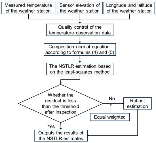
Figure 2. Flow chart of hourly NSTLR robust estimation.

As shown in Figure 2, prior to model construction, raw hourly temperature data from the 109 meteorological stations underwent a rigorous quality control procedure. This involved: (1) a range check to flag physically implausible values (<−50 °C or >50 °C); (2) a step check to identify unrealistic temporal jumps (consecutive differences > 10 °C); and (3) a climatological outlier check, where values exceeding ±5 standard deviations from the station’s long-term mean for that specific hour and month were excluded. Stations with more than 10% missing data over the study period were omitted from the analysis for that specific hour. Construct Equation (4) using the longitude, latitude, elevation, and temperature values verified by quality inspection at the meteorological station. In order to improve the accuracy of NSTLR valuation, a robust adjustment strategy is introduced.

2.3. Construction of the Grid-Based Tm Model

This study implements an elevation normalization procedure by adjusting station-observed temperatures to a common reference plane defined by the median elevation across all stations, using the derived hourly NSTLR for elevation correction. Considering the regional scope and the discrete characteristics of meteorological stations, the spatially normalized temperature field is interpolated through a Local Spherical Harmonics Interpolation Model (LSHIM) [24], which explicitly accounts for spatial autocorrelation through spectral decomposition. The LSHIM formulation represents the temperature field as

$$\left\{\begin{array}{l}{T}_r(\phi ,\lambda )={\displaystyle {\sum }_{n=1}^N{\displaystyle {\sum }_{m=0}^M\left[\Delta C_{nm}^q\cos m\lambda +\Delta S_{nm}^q\sin m\lambda \right]}}\cdot {\overline{P}}_{nm}\left(\cos \phi \right)\\ {\overline{P}}_{nm}\left(\cos \phi \right)=\sqrt{2(n+1){\displaystyle \frac{(n-m)!}{(n+m)!}}}{P}_{nm}\left(\cos \phi \right)\end{array}\right.$$

(7)

where spectral coefficients ($\Delta C_{nm}^q$, $\Delta S_{nm}^q$) characterize the temperature field’s spatial structure, $(\phi ,\lambda )$ denote geocentric coordinates, and ${\overline{P}}_{nm}$ represent the conventional Legendre polynomials. The reason for choosing sixth order ($n$ = 6) and fourth degree ($m$ = 4) spectral truncation is to best capture regional scale changes while maintaining computational efficiency [25,26]. This approach ensures physically consistent interpolation while preserving the intrinsic spatial correlation structure of the temperature field.

This study develops a multi-stage temperature interpolation framework incorporating elevation-dependent corrections. The methodology first applies a local spherical harmonics model to interpolate elevation-normalized temperatures across station locations and grid nodes, utilizing topographic data from the Advanced Spaceborne Thermal Emission and Reflection Radiometer Global Digital Elevation Model (ASTER GDEM) (https://lpdaac.usgs.gov/products/astgtmv003/ (Accepted 5 October 2025)). Systematic deviations between interpolated and NSTLR-corrected observed temperatures at station points are subsequently quantified and spatially distributed through Kriging interpolation, employing an optimized variogram model to characterize the residual spatial covariance structure. The resulting virtual temperature field at the reference elevation is then transformed to actual elevations through inverse NSTLR adjustment, expressed as $T_{actual}=T_{virtual}+\gamma \cdot \Delta E$, where $\gamma$ represents the hourly lapse rate and $\Delta E$ denotes elevation differences relative to the reference plane. Throughout this process, rigorous elevation consistency checks are maintained, including vertical datum standardization and topographic data quality control, ensuring physically meaningful temperature estimates across the entire grid domain. This approach effectively decouples the interpolation process from elevation effects while preserving the inherent spatial correlation structure of the temperature field.

3. Results

3.1. Temporal Dynamics of Hourly NSTLR

Based on robust estimation theory and observational temperature data, the hourly NSTLR across the study region was derived. However, due to inherent stochastic fluctuations in the hourly NSTLR estimates, direct analysis and application of their temporal variations are challenging. To address this issue, the study aggregates NSTLR values corresponding to the same hour over the two-year period on a monthly basis and computes their arithmetic mean. During the data consolidation process, outliers were identified and removed using a threshold of 3-fold median absolute deviation. Figure 3a–l present the temporal sequence of hourly NSTLR for all 24 h across 12 months. For comparative analysis, the ELR represented by a constant value of 0.65 °C/100 m [14], is depicted as a solid blue line in the same figure. This approach enhances the robustness of the hourly NSTLR characterization and minimizes the influence of anomalous data points.

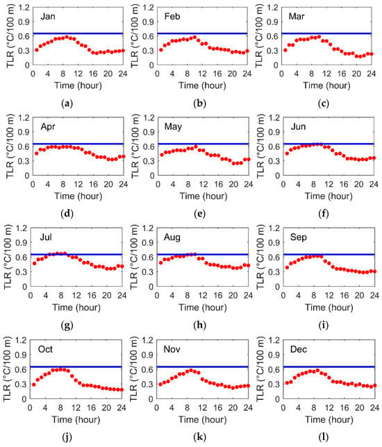
Figure 3. The time sequence of hourly NSTLR in the 12 months. The blue line represents the constant value of 0.65 °C/100 m, and the red line represents the hourly NSTLR.

As shown in Figure 3, the hourly NSTLR exhibits consistent monthly variations that predominantly remain below the constant ELR of 0.65 °C/100 m. A pronounced diurnal contrast is observed, with the most significant NSTLR differences occurring between the periods after UTC 12:00 and before UTC 04:00, where the maximum deviation reaches 0.45 °C/100 m. These findings demonstrate that directly applying the tropospheric average ELR for surface-level spatial temperature interpolation introduces substantial estimation errors relative to observed values. Such an approach particularly limits the accuracy of temperature field reconstruction in topographically complex regions, including mountainous terrain [27,28].

To systematically examine hourly NSTLR variations and their relationship with observed temperature changes, Figure 4 illustrates the temperature records from meteorological station 54,709 (116.07° E, 37.22° N; 26.90 m elevation) from 1 to 3 January 2022. Comparative analysis of Figure 3 and Figure 4 reveals a distinct positive correlation between atmospheric temperature and hourly NSTLR magnitude. At around UTC 7.2 h, the hourly NSTLR peak is approximately 0.604 °C/100 m, consistent with the highest daily temperature. At the lowest temperature, it drops to a minimum of 0.284 °C/100 m around UTC 20.5 h. This pronounced diurnal cycle demonstrates that hourly NSTLR variations exhibit strong temporal dependence on regional temperature fluctuations. Consequently, incorporating these hourly NSTLR characteristics proves essential when developing linear models for spatial grid construction and zenith-direction calculations at GNSS stations [7]. The findings highlight the importance of temporal resolution in atmospheric modeling applications, particularly for precision-dependent analyses.

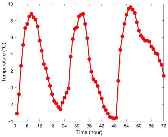
Figure 4. The hourly temperature at the meteorological station 54,709 (Longitude: 116.07°, Latitude: 37.22°, Altitude: 26.90 m) from 1 to 3 January 2022.

Table 1 presents the comprehensive statistics of hourly NSTLR variations across 24 h for each month. The analysis reveals that the 12-month average maximum NSTLR reaches approximately −0.612 °C/100 m, while the average minimum stabilizes around −0.261 °C/100 m. Examination of monthly median values demonstrates distinct seasonal patterns, with peak NSTLR magnitudes (−0.492 °C/100 m average median) occurring during the summer months (June–August). Conversely, the lowest median values (−0.323 °C/100 m) are characteristic of the winter period (November–January). Further analysis of temporal variability shows reduced NSTLR fluctuations during April–August, particularly in the peak summer months (June–August) when temperature conditions are most stable. During this period, the mean difference between maximum and minimum NSTLR values is constrained to approximately −0.297 °C/100 m. In sharp contrast, the changes in NSTLR during winter (November to January) are significantly greater, with the average range between extreme values expanding to about −0.343 °C/100 m. These patterns are visually corroborated by the temporal trends presented in Figure 3 and the statistical summary in Table 1.

Table 1. Maximum (Max.), minimum (Min.), median (Med.), and maximum minus minimum (Max. versus Min.) of hourly NSTLR for 12 months.

Month	Max.	Min.	Med.	Max. vs. Min.
1	−0.580	−0.241	−0.309	−0.339
2	−0.576	−0.250	−0.379	−0.326
3	−0.584	−0.272	−0.371	−0.312
4	−0.589	−0.275	−0.498	−0.314
5	−0.591	−0.274	−0.434	−0.317
6	−0.640	−0.330	−0.482	−0.309
7	−0.670	−0.370	−0.514	−0.301
8	−0.653	−0.373	−0.479	−0.280
9	−0.619	−0.284	−0.391	−0.335
10	−0.594	−0.282	−0.383	−0.312
11	−0.578	−0.218	−0.325	−0.360
12	−0.578	−0.243	−0.330	−0.335

The results of this study demonstrate that incorporating high spatiotemporal resolution hourly NSTLR is fundamental for developing accurate temperature grid models. Our analysis reveals significant diurnal and seasonal variations in hourly NSTLR characteristics, with diurnal fluctuations ranging between 0.284 and 0.604 °C/100 m and seasonal differences exceeding 0.15 °C/100 m between summer and winter periods. These temporal variations exhibit strong correlations with atmospheric temperature cycles (Figure 4), suggesting that conventional approaches using constant lapse rates would introduce substantial errors in temperature interpolation and extrapolation processes. Specifically, neglecting these hourly NSTLR variations during spatial modeling could lead to precision degradation exceeding 15% in complex terrain areas, as the lapse rate’s temporal dynamics directly influence surface temperature distribution patterns. Therefore, the integration of time-dependent hourly NSTLR parameters becomes particularly crucial when reconstructing high-resolution temperature fields. Especially for applications that require precise thermal characterization in areas with diverse terrains.

As shown in the above analysis, NSTLR exhibits significant seasonal and diurnal variations. From a physical perspective, seasonal changes may be related to the thermal conditions of the atmosphere. In summer, solar radiation is strong, surface heating is intense, and convective activity is vigorous, resulting in a faster decrease in temperature with altitude. In winter, the opposite is true, with a relatively stable atmospheric structure. In terms of daily variation, the heating of the sun during the day leads to the development of convection, while radiation cooling at night forms a stable boundary layer, which affects the vertical structure of temperature. As for altitude dependence, the atmosphere in high-altitude areas is thinner, and their response to solar radiation is different. Moreover, the terrain is usually more complex, and local circulation can affect temperature distribution.

3.2. Development and Validation of the Grid-Based Model

An hourly resolution $T_m$ grid model was established by using the hourly NSTLR across 12 months, along with hourly measured temperature (represented by the blue dots in Figure 2). The detailed construction of the $T_m$ grid model is described in Section 2.1. The resulting model outputs gridded values with a spatial resolution of 0.15° × 0.15°, as exemplified by the spatial distribution of values at 00:00 UTC on 31 December 2022 (Figure 5). The gridded parameters exhibit a regional range of 260–278 K (mean: 271.83 K), demonstrating strong correspondence with actual surface temperature patterns while maintaining dynamic temporal variability. For GNSS precipitable water vapor calculations, spatial interpolation of the four nearest grid points enables accurate parameter estimation at individual station locations [21].

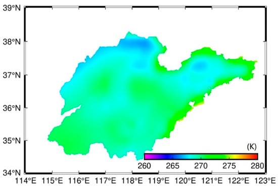
Figure 5. The spatial distribution of $T_m$ values at UTC 0 h on 31 December 2022.

The verification process employed the same linear regression model between $T_s$ and $T_m$ to compute hourly $T_m$ values from meteorological station temperature measurements, establishing reference data for validation. The methodology involved extracting $T_m$ values from the four nearest grid points to each validation station, followed by bilinear interpolation to derive station-specific estimates. These interpolated values were then compared against direct calculations from observed temperatures. To comprehensively assess performance, three distinct methodologies were implemented: (1) uncorrected grid-point calculations, (2) correction using the standard ELR of 0.65 °C/100 m [21], and (3) correction incorporating the hourly NSTLR values derived in this study. All approaches maintained consistent $T_m$ and $T_s$ conversion coefficients. This comparative framework was designed to both evaluate elevation-dependent temperature interpolation accuracy and quantify the improvement achieved through the proposed NSTLR correction method.

Figure 6a–d present the hourly time series of $T_m$ derived from the three schemes alongside values calculated from actual surface temperature measurements at four meteorological stations of varying elevations. Comparative analysis reveals that the hourly NSTLR-corrected scheme outperforms both the uncorrected and ELR-corrected approaches. The enhancement exhibits a positive correlation with station elevation, showing particularly significant improvement over the uncorrected model in high-altitude locations. Notably, minimal divergence occurs among the three methods at low-elevation stations (top-left subplot), where all curves exhibit near-identical behavior, indicating negligible elevation-dependent effects in these areas. It is worth noting that in order to clearly distinguish the temporal variations in Tm calculated by various models, in each subgraph of Figure 6, the green, cyan, and red colors are offset by+5, −5, and −10 K, respectively.

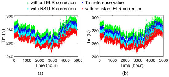
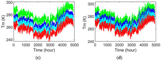
Figure 6. The $T_m$ time series under different schemes. (a) The elevation is 5.70 m; (b) The elevation is 118.70 m; (c) The elevation is 1536.50 m; (d) The elevation is 303.70 m. Green, cyan, and red are biased by +5, −5, and −10 K, respectively.

To quantitatively evaluate the three grid models, we calculated root mean square errors (RMSE) and bias between interpolated and reference values $T_m$ derived from meteorological stations, stratified by four elevation intervals (Figure 7 and Table 2). The uncorrected model showed the poorest performance, with maximum RMSE (6.53 K) at high-elevation Tai Shan station, decreasing to 1.00 K in low-altitude regions. TLR correction substantially improved model accuracy, with constant ELR correction reducing RMSE by 47.5%, 24.7%, 16.3%, and 7.1% across elevation intervals compared to the uncorrected model. Further refinement using hourly NSTLR correction yielded additional RMSE reductions of 0.72 K, 0.13 K, 0.06 K, and 0.05 K, respectively, and the accuracy improvements of 21.1%, 11.3%, 6.3%, and 5.4% over the ELR-corrected model. These results demonstrate that elevation-dependent correction, particularly using temporally resolved NSTLR, progressively enhances interpolation accuracy with increasing terrain elevation.

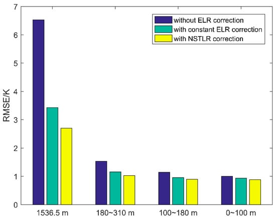
Figure 7. The RMSE of the $T_m$ interpolation residuals for the three approaches at four elevation intervals.

Table 2. The average RMSE and bias values for different elevation intervals and correction method.

	Elevation Intervals (m)	1536.5	180~350	100~180	0~100
RMSE	Without ELR correction (K)	6.53	1.54	1.14	1.00
	With constant ELR correction (K)	3.43	1.16	0.96	0.93
	With NSTLR correction (K)	2.70	1.02	0.89	0.88
	Without ELR correction/With NSTLR correction	58.65%	33.77%	21.93%	12.00%
	With constant ELR correction/With NSTLR correction	21.28%	12.07%	7.29%	5.38%
Bias	Without ELR correction (K)	4.83	2.28	1.77	0.80
	With constant ELR correction (K)	3.55	1.30	0.90	0.43
	With NSTLR correction (K)	0.65	0.35	0.23	0.16
	Without ELR correction/With NSTLR correction	65.84%	54.33%	29.06%	28.00%
	With constant ELR correction/With NSTLR correction	53.52%	26.92%	25.89%	16.28%

Figure 8 presents the diurnal variation of 24 h averaged RMSE for the three models, obtained by temporally averaging errors across all validation stations. The uncorrected model demonstrates consistently higher errors (mean RMSE around 1.58 K), while the TLR-corrected versions show marked improvement. Notably, the hourly NSTLR-corrected model achieves superior performance with a minimum daily mean RMSE of 0.91 K. Temporal analysis reveals distinct diurnal patterns: during UTC 04:00–10:00, the difference between constant ELR and NSTLR corrections becomes negligible (mean RMSE difference: 0.042 K), whereas other periods exhibit greater divergence (maximum RMSE difference: 0.157 K). These results indicate that although both TLR correction methods improve model accuracy, the temporal-resolution NSTLR approach delivers optimal performance, especially outside morning periods.

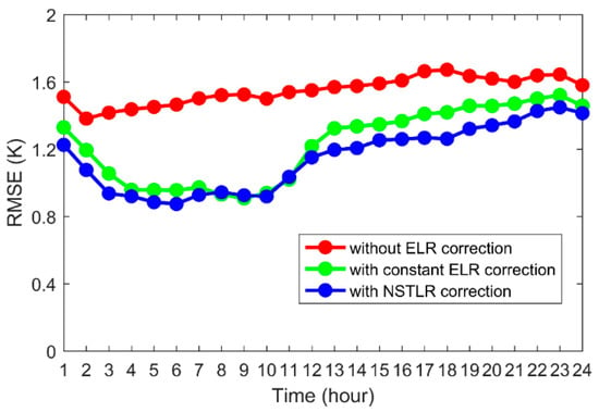
Figure 8. The hourly statistics of the RMSE of three $T_m$ grid models for the entire region.

Comparative analysis with Figure 3 reveals that the diurnal variation in performance between the two TLR-corrected grid models exhibits strong correspondence with the temporal characteristics of hourly NSTLR. The divergence between model outputs intensifies proportionally with increasing discrepancy between NSTLR and constant ELR values. This correlation demonstrates that direct application of ELR for surface temperature interpolation introduces systematic errors that vary temporally with NSTLR-ELR differences. The proposed hourly NSTLR-corrected model successfully captures these temporal dynamics, enabling accurate representation of $T_m$’s diurnal variations through its high-temporal-resolution framework. These findings confirm that conventional ELR-based approaches cannot adequately account for the time-dependent nature of near-surface temperature lapse processes.

4. Discussion

4.1. Cross-Validation with ERA5 Reanalysis Dataset

This study employs a dual validation approach for the grid model evaluation. While the initial accuracy assessment utilized meteorological station measurements for internal consistency verification, we further conducted external validation using ERA5 reanalysis data (0.25° × 0.25° spatial resolution, hourly temporal resolution) obtained from the Copernicus Climate Data Store. The ERA5 dataset, comprising 37 pressure-level atmospheric variables (including temperature, humidity, and specific humidity from 1000 hPa to 1 hPa), enabled independent verification through bilinear interpolation of reference values to our model grid points. Given the demonstrated deficiencies in uncorrected models (Section 3), the comparative analysis focused on two approaches: Scheme A (hourly NSTLR-corrected) and Scheme B (constant ELR-corrected), with performance evaluated through RMSE analysis of interpolated residuals.

Figure 9 illustrates the spatial distribution of mean RMSE for $T_m$ residuals in Scheme A (panel a) and Scheme B (panel b), with corresponding elevation-stratified statistics presented in Table 3. Both schemes demonstrate RMSE ranges of 1.30–3.90 K across elevation zones, consistent with radiosonde-based validation results reported by Xu et al. [28]. Due to data availability constraints from the University of Wyoming’s radiosonde network during our study period (http://weather.uwyo.edu/wyoming/ (accessed on 10 October 2025)), ERA5 reanalysis data served as the validation benchmark [29,30]. The analysis reveals systematic elevation-dependent errors, with maximum RMSE differences between high and low elevation regions reaching 1.38 K (Scheme A) and 2.18 K (Scheme B). Notably, the hourly NSTLR correction in Scheme A reduces elevation-dependent biases more effectively than constant ELR correction (Scheme B), particularly in high-altitude areas where RMSE improvements reach 1.12 K. Regional average analysis shows Scheme A achieves a 0.73 K mean RMSE reduction (19.4% accuracy improvement) compared to Scheme B, demonstrating the critical importance of temporally resolved NSTLR for precise temperature field reconstruction, especially in topographically complex regions.

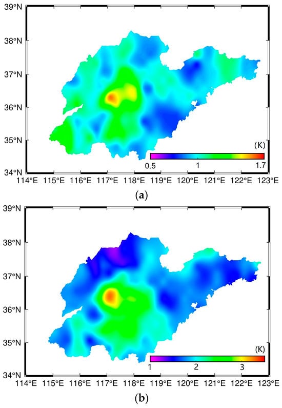
Figure 9. The spatial distribution of average RMSE for $T_m$ residuals. (a) Scheme A; (b) Scheme B.

Table 3. The average RMSE values for different elevation intervals.

Elevation Intervals (m)	1536.5	180~350	100~180	0~100
Scheme A (K)	2.77	1.70	1.41	1.39
Scheme B (k)	3.89	2.17	1.53	1.48
Accuracy improvement ratio	28.79%	21.66%	7.84%	6.08%

While the ERA5 reanalysis dataset serves as a valuable and widely used benchmark for independent validation, it is important to acknowledge its known limitations in regions of complex topography, such as mountainous areas. The model’s inherent spatial smoothing and potential biases in representing fine-scale orographic processes mean that the absolute RMSE values reported here should be interpreted with caution, as they may not represent the absolute ground truth. However, the primary objective of this comparative analysis was to evaluate the relative performance of Scheme A (hourly NSTLR) against Scheme B (constant ELR) under a consistent validation framework. The significant and systematic reduction in RMSE achieved by Scheme A across all elevation intervals, even when validated against a dataset that might itself be imperfect, provides strong and conservative evidence for its superiority. If ERA5 exhibits smoothing that dampens actual atmospheric variability, the demonstrated improvement of our method might, in fact, be an underestimate. Therefore, the comparative results robustly affirm that the integration of temporally resolved NSTLR is critical for enhancing the accuracy of $T_m$ modeling in topographically complex regions, outperforming the conventional constant ELR approach irrespective of the inherent uncertainties in the validation dataset.

4.2. Inter-Regional Validation of the Grid Model Methodology

In order to comprehensively evaluate the proposed grid modeling method, we conducted additional validation studies in two different geographical regions: Sichuan Province in southwestern China. The Sichuan validation utilized hourly meteorological data from 145 uniformly distributed stations (Figure 10) during 23 September–23 October 2022. The region’s pronounced topographic gradient ranging from 160 m in eastern lowlands to 6500 m in western highlands (Figure 10 elevation shading)—provides an ideal testbed for evaluating the model’s performance across extreme elevation variations. This heterogeneous terrain configuration offers rigorous conditions for validating the robustness of the grid modeling approach in handling complex orographic features.

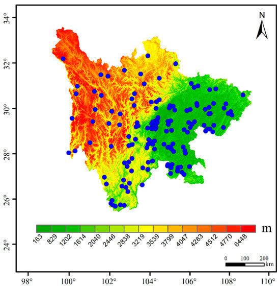
Figure 10. Distribution of topography and meteorological stations in Sichuan Province in southwestern China.

The hourly NSTLR was derived from meteorological station observations (longitude, latitude, elevation, and temperature) using Equations (4)–(6). To ensure the reliability of the solution, the same quality control procedures as those analyzed in Shandong Province were adopted. Figure 11 compares the diurnal NSTLR cycle (red dashed line) against the constant ELR (0.65 °C/100 m, blue line). Despite significant geographical separation and topographic differences between Sichuan and Shandong provinces, both regions exhibit remarkably similar NSTLR temporal patterns. The hourly NSTLR values remain consistently below the constant ELR threshold, displaying a characteristic diurnal cycle that peaks at 0.616 °C/100 m (before 10:00 UTC) and reaches a minimum of 0.467 °C/100 m. This pattern demonstrates a consistent positive correlation between hourly NSTLR magnitude and atmospheric temperature across both study regions, with hourly NSTLR increasing during warming periods and decreasing during cooling phases.

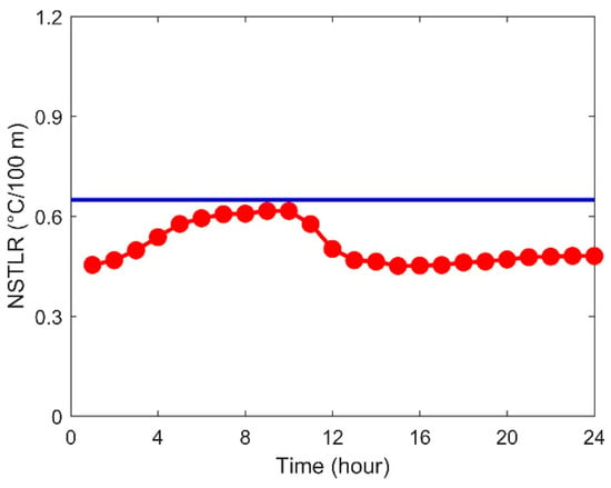
Figure 11. The hourly NSTLR time sequence for each of the 24 h (red dotted line) and constant ELR (blue line).

The grid modeling methodology followed the same approach as applied in Shandong Province. Temperature observations were first elevation-corrected to a reference plane (1599.3 m, corresponding to the median station elevation) using hourly NSTLR, then spatially interpolated to 0.15° × 0.15° grid points via Equation (7). Gridded $T_m$ values were subsequently derived using the global latitude-dependent regression model from Yao et al. [19]. Model validation involved: (1) bilinear interpolation of grid values back to station locations, and (2) comparison with station-based T_m calculations through RMSE analysis. Figure 12 shows the average RMSE for five elevation difference intervals under two strategies. The detailed statistical information is summarized in Table 4. Comparative evaluation with constant-ELR models revealed significant accuracy improvements when using hourly NSTLR, with RMSE values of 1.07 K (0–200 m), 1.52 K (200–500 m), 2.14 K (500–1000 m), 2.44 K (1000–2000 m), and 2.88 K (2000–2700 m). The accuracy can be improved by 9.69%, 15.92%, 26.45%, 30.46% and 35.88% for these five elevation difference intervals, respectively. These results confirm both the robustness of the proposed methodology and its superior performance relative to conventional ELR-based approaches.

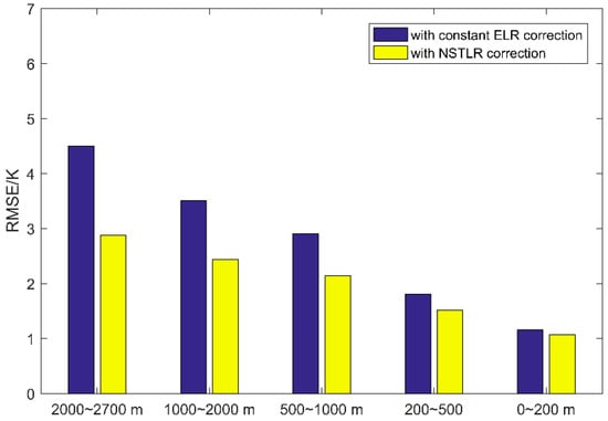
Figure 12. The average RMSE for five elevation difference intervals under two strategies.

Table 4. The average RMSE values for different elevation intervals and correction method.

Elevation Intervals (m)	2000~7000	1000~2000	500~1000	200~500	0~200
With constant ELR correction (k)	4.49	3.51	2.91	1.81	1.18
With NSTLR correction	2.88	2.44	2.14	1.52	1.07
Accuracy improvement ratio	35.86%	30.48%	26.46%	16.02%	35.86%

4.3. Limitations and Future Perspectives Under Nocturnal Inversion Conditions

Although the proposed hourly NSTLR-based grid model achieves notable accuracy improvements in topographically complex regions, its performance may degrade under certain meteorological conditions, such as nocturnal radiative inversions. Under clear-sky and calm-wind conditions, a stable boundary layer develops, leading to an increase in temperature with height near the surface, which contradicts the fundamental assumption of a negative temperature lapse rate underpinning our model. During such events, the estimated NSTLR from multiple linear regression may yield anomalous values or even reverse its sign, consequently impairing the accuracy of the elevation normalization and the subsequent spatial interpolation of the temperature field. Furthermore, the current model, relying solely on surface station data, might not fully resolve the intricate three-dimensional thermal structure within the inversion layer.

Future research will focus on enhancing the model’s adaptability to stable boundary layer conditions (including, but not limited to, nocturnal inversions, convective instability events, or fronts). Potential avenues for improvement include: (1) incorporating real-time or forecasted boundary layer height data to dynamically identify the occurrence and intensity of inversions; (2) assimilating satellite-derived land surface temperature data (e.g., from MODIS), which is sensitive to cold-air pooling effects caused by nocturnal surface cooling; and (3) introducing meteorological covariates such as wind speed and cloud cover into the NSTLR estimation to better discriminate between normal lapse and inversion regimes. Despite this limitation, the high spatiotemporal resolution NSTLR framework established in this study provides a solid foundation for future integration of multi-source data towards developing a more robust atmospheric temperature modeling approach.

5. Conclusions

This study developed a novel high-resolution grid modeling methodology for $T_m$ incorporating hourly NSTLR corrections. The key innovations include a robust estimation strategy for deriving time-varying hourly NSTLR and an optimized spatial interpolation framework that decouples elevation effects from the temperature field. The approach also offers enhanced data privacy by disseminating gridded products without disclosing exact station locations.

Comprehensive validations across Shandong Province and Sichuan Province demonstrate that the proposed NSTLR-corrected $T_m$ grid model achieves significant accuracy improvements over both uncorrected and constant ELR-corrected models, particularly in high-altitude areas. The results confirm the practical significance and effectiveness of the proposed method for $T_m$ construction using ground-based meteorological observations in regions with large terrain changes, similar to the tested areas.

The proposed grid-based $T_m$ model shows considerable potential for operational integration into GNSS meteorology. The computational load is manageable, which determines the number of weather stations and the estimated frequency of NSTLR. Processing an hour’s worth of time on a standard computer only takes a few minutes and can generate $T_m$ fields in near real-time. This model relies solely on conventional available surface temperature observations and can be directly implemented in existing meteorological data processing chains. While the model shows great promise, its applicability to contrasting climatic regimes (e.g., arid or polar regions) and under all seasonal weather phenomena (e.g., persistent temperature inversions) should be systematically evaluated in future work. Nevertheless, the proposed model demonstrates strong potential for operational integration in GNSS meteorology. Its manageable computational load and reliance on conventional surface temperature observations make it suitable for generating near real-time, high-precision PWV products, which are crucial for nowcasting and severe weather monitoring.

References

- Zhang, W.; Zhang, H.; Liang, H.; Lou, Y.; Cai, Y.; Cao, Y.; Zhou, Y.; Liu, Y. On the suitability of ERA5 in hourly GPS precipitable water vapor retrieval over China. J. Geod. 2019, 93, 1897–1909. [Google Scholar] [CrossRef]
- Bevis, M.; Businger, S.; Chiswell, S.; Herring, T.; Anthes, R.; Rocken, C.; Ware, R. GPS meteorology: Mapping zenith wet delays onto precipitable. J. Appl. Meteorol. 1994, 33, 379–386. [Google Scholar] [CrossRef]
- Bevis, M.; Businger, S.; Herring, T.; Rocken, C.; Anthes, R.; Ware, R. GPS meteorology: Remote sensing of the atmospheric water vapor using the global positioning system. J. Geophys. Res. 1992, 97, 15787–15801. [Google Scholar] [CrossRef]
- Wang, X.; Song, L.; Dai, Z.; Cao, Y. Feature analysis of weighted mean temperature Tm in Hong Kong. J. Nanjing Univ. Inf. Sci. Technol. 2011, 3, 47–52. [Google Scholar] [CrossRef]
- Yao, Y.; Zhang, B.; Xu, C.; Yan, F. Improved one/multiparameter models that consider seasonal and geographic variations for estimating weighted mean temperature in ground-based GPS meteorology. J. Geod. 2014, 88, 273–282. [Google Scholar] [CrossRef]
- Yang, F.; Guo, J.; Meng, X.; Li, J.; Li, Z.; Tang, W. GGTm-Ts: A global grid model of weighted mean temperature (Tm) based on surface temperature (Ts) with two modes. Adv. Space Res. 2023, 71, 1510–1524. [Google Scholar] [CrossRef]
- Yao, Y.; Zhu, S.; Yue, S. A globally applicable, season-specific model for estimating the weighted mean temperature of the atmosphere. J. Geod. 2012, 86, 1125–1135. [Google Scholar] [CrossRef]
- Huang, L.; Jiang, W.; Liu, L.; Chen, H.; Ye, S. A new global grid model for the determination of atmospheric weighted mean temperature in GPS precipitable water vapor. J. Geod. 2019, 93, 159–176. [Google Scholar] [CrossRef]
- Sun, Z.; Zhang, B.; Yao, Y. A global estimation tropospheric delay and weighted mean temperature developed with atmospheric reanalysis data from 1979 to 2017. Remote Sens. 2019, 11, 1893. [Google Scholar] [CrossRef]
- Landskron, D.; Böhm, J. VMF3/GPT3: Refined discrete and empirical troposphere mapping functions. J. Geod. 2018, 92, 349–360. [Google Scholar] [CrossRef]
- Zhang, K.; Li, H.; Wang, X.; Zhu, D.; He, Q.; Li, L.; Hu, A.; Zheng, N.; Li, H. Recent progresses and future prospective of ground-based GNSS water vapor sounding. Acta Geod. Cratographica Sin. 2022, 51, 1172–1191. (In Chinese) [Google Scholar]
- Zhou, C.; He, Y.; Wang, K. On the suitability of current atmospheric reanalyses for regional warming studies over China. Atmos. Chem. Phys. 2018, 18, 8113–8136. [Google Scholar] [CrossRef]
- Zhao, T.; Guo, W.; Fu, C. Calibrating and evaluating reanalysis surface temperature error by topographic correction. J. Clim. 2008, 21, 1440–1446. [Google Scholar] [CrossRef]
- Zeng, H.; Tian, P.; Zhang, M.; Cao, X.; Liang, J.; Zhang, L. Rapid change in surface-based temperature inversions across the world during the last three decades. J. Appl. Meteorol. Climatol. 2022, 61, 175–184. [Google Scholar] [CrossRef]
- Wang, L.; Sun, L.; Shrestha, M.; Li, X.; Liu, W.; Zhou, J.; Yang, K.; Lu, H.; Chen, D. Improving snow process modeling with satellite-based estimation of near-surface-air-temperature lapse rate. J. Geophys. Res. Atmos. 2016, 121, 12005–12030. [Google Scholar] [CrossRef]
- Ojha, R. Assessing seasonal variation of near surface air temperature lapse rate across India. Int. J. Climatol. 2017, 37, 3413–3426. [Google Scholar] [CrossRef]
- Karki, R.; Hasson, S.; Schickhoff, U.; Scholten, T.; Böhner, J.; Gerlitz, L. Near surface air temperature lapse rates over complex terrain: A WRF based analysis of controlling factors and processes for the central Himalayas. Clim. Dyn. 2020, 54, 329–349. [Google Scholar] [CrossRef]
- Zhong, H.; Zhou, J.; Tang, W.; Zhou, G.; Wang, Z.; Wang, W.; Meng, Y.; Ma, J. Estimation of Near-Surface Air Temperature Lapse Rate Based on MODIS Data Over the Tibetan Plateau. IEEE J. Sel. Top. Appl. Earth Obs. Remote Sens. 2023, 16, 4767–4777. [Google Scholar] [CrossRef]
- Yao, Y.; Zhang, B.; Xu, C.; Chen, J. Analysis of the global Tm−Ts correlation and establishment of the latitude-related linear model. Chin. Sci. Bull. 2014, 59, 2340–2347. [Google Scholar] [CrossRef]
- Ross, R.; Rosenfeld, S. Estimating mean weighted temperature of the atmosphere for Global Positioning System applications. J. Geophys. Res. 1997, 102, 21719–21730. [Google Scholar] [CrossRef]
- Li, X.; Wang, L.; Chen, D.; Yang, K.; Xue, B.; Sun, L. Near-surface air temperature lapse rates in the mainland China during 1962–2011. J. Geophys. Res. Atmos. 2013, 118, 7505–7515. [Google Scholar] [CrossRef]
- He, Y.; Wang, K. Contrast patterns and trends of lapse rates calculated from near-surface air and land surface temperatures in China from 1961 to 2014. Sci. Bull. 2020, 65, 1217–1224. [Google Scholar] [CrossRef] [PubMed]
- Wang, L.; Ma, J.; Zhao, X.; Li, X.; Zhang, K.; Jiao, Z. Adaptive robust unscented Kalman filter-based state-of-charge estimation for lithium-ion batteries with multi-parameter updating. Electrochim. Acta 2022, 426, 140760. [Google Scholar] [CrossRef]
- Jin, R.; Jin, S.; Feng, G. M_DCB: Matlab code for estimating GNSS satellite and receiver differential code biases. GPS Solut. 2012, 16, 541–548. [Google Scholar] [CrossRef]
- Zhou, C.; Yang, L.; Li, B.; Balz, T. M_GIM: A MATLAB-based software for multi-system global and regional ionospheric modeling. GPS Solut. 2023, 27, 42. [Google Scholar] [CrossRef]
- Yue, C.; Hu, L.; Yan, Y. Estimation on the hourly near-surface temperature lapse rate and its time-varying characteristics. Heliyon 2024, 10, e31964. [Google Scholar] [CrossRef] [PubMed]
- Blandford, T.; Humes, K.; Harshburger, B.; Moore, B.; Ye, H. Seasonal and synoptic variations in near-surface air temperature lapse rates in a mountainous basin. J. Appl. Meteorol. Climatol. 2008, 47, 249. [Google Scholar] [CrossRef]
- Xu, M.; Guo, Q.; Hou, J.; Sun, Y.; Li, D. Modeling and accuracy analysis of weighted mean temperature in Jinan region. J. Navig. Position. 2021, 9, 142–151. (In Chinese) [Google Scholar]
- Yue, C.; Wang, H.; Hu, L.; Dang, Y.; Wang, Y. Evaluation and refinement of ERA5-land 2 m atmospheric temperature in GNSS precipitable water vapor. Adv. Space Res. 2024, 74, 4639–4654. [Google Scholar] [CrossRef]
- Yue, C.; Wang, H.; Xu, C. Augmentation Method for Weighted Mean Temperature and Precipitable Water Vapor Based on the Refined Air Temperature at 2 m above the Surface of Land from ERA5. Remote Sens. 2024, 16, 2055. [Google Scholar] [CrossRef]
Disclaimer/Publisher’s Note: The statements, opinions and data contained in all publications are solely those of the individual author(s) and contributor(s) and not of MDPI and/or the editor(s). MDPI and/or the editor(s) disclaim responsibility for any injury to people or property resulting from any ideas, methods, instructions or products referred to in the content. |
© 2025 by the authors. Licensee MDPI, Basel, Switzerland. This article is an open access article distributed under the terms and conditions of the Creative Commons Attribution (CC BY) license (https://creativecommons.org/licenses/by/4.0/).