Abstract
We analyze the relation between maximum tropospheric ozone concentration and surface temperature in Mexico City between 2000 and 2021. Changes in ozone levels over the decades appear to respond to public strategies aimed at reducing its precursors. The exponential fit between temperature and maximum ozone concentration is [O3] = 9.33 × exp (0.0957 × T), with a coefficient of determination of 0.73, for the period 2000–2021. Reordering the data by five-year period improves the fit slightly; the intercepts increase from 8.431 (2000–2004) to 10.428 (2015–2019), and the slopes decrease from 0.1051 (2000–2004) to 0.0839 (2015–2019), providing a quantitative insight into how public strategies and policies modify air pollution and make Mexico City’s atmosphere less reactive.
1. Introduction
Ozone (O3) is a key component of the Earth’s atmosphere, playing a complex role in the Earth’s climate system as both a greenhouse gas and a pollutant. Natural processes and human activities influence its concentration in the lower atmosphere. Tropospheric O3 is not directly emitted into the atmosphere. Instead, it is formed through complex chemical reactions involving precursor pollutants, primarily nitrogen oxides (NOx) and volatile organic compounds (VOCs). The O3 formation reactions are often facilitated by solar radiation with wavelengths less than 340 nm [1]. The rate of formation can also be influenced by temperature, with higher temperatures generally leading to an increase in the O3 production. This relationship is significant in urban areas with high emissions of O3 precursors [2]. Although the exact mechanism relating temperature and O3 may vary by region, the most relevant factors are likely the temperature-dependent chemical rate constants, the relationship between stagnation events and temperature, the changes in meteorological parameters associated with elevated temperatures, and temperature-dependent emissions (e.g., biogenic emissions).
Additionally, a reduction in NOx emissions can lead to an increase in ozone concentrations in situations where VOC-driven photochemical reactions encourage ozone production at the surface, and stagnant meteorological conditions promote and maintain ozone events [3]. Thus, the association between stagnant air masses and warm temperatures will facilitate the accumulation of O3 precursors.
O3 concentration also depends on meteorological factors (wind speed, planetary boundary layer height, relative humidity, clouds, and precipitation), which modify its distribution in relation to other pollutants [4,5]. According to the literature, higher temperature levels can increase the O3 concentration through its direct effect on O3 accumulation [6,7], and through an indirect effect on nitrogen and other variables, which, in turn, affects the O3 concentration [8,9,10,11,12,13]. While temperature plays a critical role in enhancing photochemical oxidation rates and biogenic VOC emissions, it is not the sole meteorological driver of ozone formation. Transport processes, boundary layer height, cloud cover, ventilation efficiency, and precipitation scavenging also modulate ozone concentrations in polluted environments. These mechanisms have been documented in other megacities experiencing strong photochemical regimes, including Los Angeles, Beijing, and Athens [5,14,15]. In this study, temperature is isolated to quantify long-term nonlinear sensitivity, while acknowledging that a full meteorological attribution requires a multivariate framework.
Warmer temperatures can contribute to the formation and accumulation of pollutants, including O3, exacerbating air quality issues. Previous work has identified increasing temperatures as a driver of elevated surface O3 concentrations, mitigating the effectiveness of ongoing emissions reductions in the United States and Europe [3,16,17]. That means, under a warming climate, polluted regions would need to cut emissions even further to achieve the same improvement in air quality, adding economic and human health costs to the bottom line of climate change adaptation.
Megacities such as Mexico City represent ideal environments for studying ozone–temperature interactions due to their VOC-limited photochemical regime, high precursor emissions, strong solar radiation, and intensified heat-island effects. These characteristics make the region particularly sensitive to climate-driven increases in temperature, similarly to observations reported in Los Angeles, Beijing, and European industrial basins [3,14,18]. In this paper, we analyze how these interactions evolved under changing precursor emissions and successive air-quality policies.
In Mexico City, we have high concentrations of O3 in winter (December–January) and spring (April–May). Days with clear skies and strong isolation in the morning hours promote the rapid generation of O3 via photochemical conversions [19]. So, we considered Mexico City a closed system with two feedback loops: (1) between UV radiation and relative humidity, which may affect the O3 concentration [20,21,22,23,24], and (2) the reaction of nitrogen oxides to produce O3. In addition, in this system, the relative humidity has an indirect effect on the concentration of O3 through its effects on nitrogen oxides [7,25].
Temperature is the most common parameter used to describe events related to global warming; for this reason, we employed it to illustrate the trend of maximum tropospheric ozone concentrations in Mexico City, given its implications for climate change and air quality in large cities and megacities. Also, the air quality in densely populated metropolitan areas, like Mexico City, exhibits a significant environmental challenge because it is influenced by several factors (geographical location, demography, meteorology, atmospheric processes, level of industrialization, and socioeconomic development) [14,26].
This study contributes by (i) quantifying a 21-year nonlinear relationship between ozone and surface temperature, (ii) comparing exponential fits across successive environmental governance cycles, and (iii) interpreting the temperature-sensitivity coefficient b as an indicator of atmospheric reactivity that decreases under declining precursor emissions. To our knowledge, this is the first long-term assessment linking reduced temperature sensitivity to policy-driven emission declines in Mexico City.
Thus, we aim to describe the relationship between tropospheric O3 and surface temperature in Mexico City from 2000 to 2021. Given that it is a complex issue, we analyzed it in a multivariate framework. We used two types of regression models: (1) a multivariate time series vector autoregression model [27,28] that not only includes O3 and temperature but also incorporates other variables associated with O3 concentration, such as nitrogen oxides, radiation, and environmental 5-year policy shocks using dichotomous variables that capture temporary changes in environmental policy in Mexico City [29]. And (2) a bivariate nonlinear regression model, which only includes tropospheric O3 and surface temperature. The exponential function was selected to model the relationship between O3 and temperature, based on the Arrhenius-type temperature dependence of photochemical reaction rates governing O3 production [2]. This methodological approach allowed us to validate the statistical robustness of our results regarding the bivariate relationship between tropospheric O3 and surface temperature.
2. Materials and Methods
Since 1986, the Automatic Atmospheric Monitoring Network (RAMA) and the Meteorology and Solar Radiation Network (REDMET) have measured air pollutants and meteorological parameters in Mexico City. RAMA has 40 stations recording hourly atmospheric pollutants (CO, NO, NO2, NOx, O3, SO2, PM10, and PM2.5). Figure 1 shows the location of RAMA stations. Information about the RAMA and REDMET instrumentation is in Supplementary Material, Table S1.
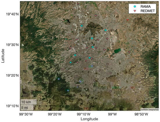
Figure 1.
Location of air quality monitoring stations with meteorological parameters in Mexico City.
REDMET has 28 stations that measure surface temperature, relative humidity, wind speed and direction, and solar radiation. RAMA and REDMET data portal at http://www.aire.cdmx.gob.mx/ (last visit 31 January 2022) provide access to download both the average hourly data of pollutant concentrations and meteorological parameters.
RAMA pollutant observations were collected hourly following SEDEMA QA/QC protocols. Data flagged for calibration, maintenance, or instrumental drift were removed, along with missing periods longer than three consecutive hours. REDMET temperature data were paired to the nearest RAMA station within 5 km to ensure meteorological representativeness. Figure 1 now displays stations with both air quality and meteorological data. Spatial mismatches remain a limitation and are acknowledged explicitly.
2.1. Statistical Analyses and Data Processing
The bivariate analysis between O3 and surface temperature in a nonlinear regression model (exponential regression estimation) uses the maximum daily concentrations of O3 and the maximum daily temperature (from 2000 to 2021) to perform the calculations.
In addition, to reinforce the results of our bivariate nonlinear model, we also estimated the effects of surface temperature on tropospheric O3 using a multivariate time series model. We estimated a vector autoregression (VAR) model using daily data series, which included O3, temperature, nitrogen oxides, relative humidity, UV-A, and UV-B. We also included five dichotomous variables that capture the temporary effects of five-year policy changes in Mexico City, which take the value of one for every five years and zero otherwise. The VAR model enabled us to demonstrate the effects of temperature and other potential precursors on O3 by estimating impulse response functions and conducting a variance decomposition analysis [25,26]. This modelling approach allowed us to consistently approximate the role played by different precursors and their interactions in the system. A VAR(p) model was estimated after verifying stationarity using augmented Dickey–Fuller tests. Lag length selection followed Akaike (AIC) and Schwarz (SIC) criteria. Cholesky decomposition ordering placed O3 first to isolate structural shocks [25,26]. Impulse-response functions were computed using a 10-day horizon to capture short-term interactions between temperature and ozone. Data analysis was conducted using EViews version 12 and MATLAB version 2021.
2.2. Meteorological Parameters
The maximum temperature recorded in the Mexico City Metropolitan Area has been increasing gradually over time. In 2000, the maximum temperature recorded was 32.5 °C, and by 2021, it had risen to 33.2 °C, representing a rate of 0.2 °C per year. Although the maximum temperatures were not recorded at the same point, they are likely subject to similar conditions (i.e., low tree density, high population density, vehicular traffic, and buildings). The measurements reflect the overall impact of urban growth in Mexico City and the corresponding increase in the region’s average temperature.
2.3. Ozone Trends and Precursors Abatement Strategies
Mexico City authorities have a Contingency Plan to reduce tropospheric O3 in the region when it reaches threshold values. Between 1990 and 2006, a Phase I contingency was decreed at 265 ppb. Since then, the threshold has been gradually lowered. In 2012, it was established at 194 ppb, and in 2016 at 155 ppb (Figure 2). Current Mexico City Phase I contingency thresholds are 155 ppb (1 h), consistent with local health risk protocols. Between 1990 and 2010, the average O3 concentration had a downward trend; however, starting in 2010, that trend has stalled. The maximum O3 concentration over time suggests a decreasing trend every five years, which is likely associated with the environmental policy measures implemented by the local government. Five-year maximum O3 were classified with letters, and Table 1 shows the main actions applied at each time.
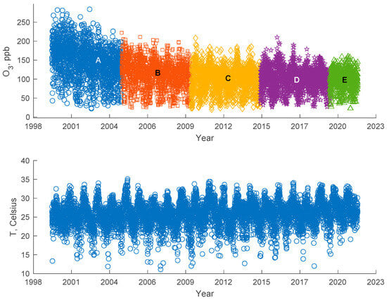
Figure 2.
Maximum ozone concentrations and surface temperatures since 2000. Capital letters correspond to actions implemented to reduce precursor emissions and improve the air quality.

Table 1.
Actions to reduce ozone precursors.
These five periods correspond to successive phases of Mexico City’s ProAire environmental programs (2000–2004, 2005–2009, 2010–2014, 2015–2019, 2020–2021), each associated with major policy interventions affecting precursor emissions, including fuel sulfur reductions and transportation modernization. To test robustness, a two-period analysis (2000–2009 vs. 2010–2021) was additionally performed, yielding consistent exponential behavior (Supplementary Material Figure S1 and Table S2).
Despite the stricter limits established over the years to apply environmental contingency measures and protect the population from exposure to excessively high O3 levels, the results have not shown the expected rate of reduction compared to the previous years. Table 1 lists the most relevant actions implemented over 20 years to reduce O3 precursors, as well as others aimed at improving public transportation. The actions are aimed at public transport and private cars, without considering other sectors that contribute to precursor emissions (i.e., industries and domestic sources). However, these environmental policy actions yielded positive results and altered the trends in O3 concentrations in Mexico City.
Linear trend analysis of maximum daily ozone concentrations shows a strong decline during 2000–2004 (−10.35 ppb year−1), followed by a moderate decrease during 2005–2009 (−3.72 ppb year−1), a weaker decline in 2010–2014 (−0.83 ppb year−1), and near-stability in 2015–2019 (−0.30 ppb year−1). For 2021, the trend is near zero (+0.02 ppb year−1), reflecting post-pandemic stabilization. These results suggest diminishing marginal benefits from precursor reductions as the atmosphere becomes less reactive under a VOC-limited regime.
A linear regression on annual maximum temperature yields a warming trend of +0.04 °C/year (R2 = 0.41, p < 0.01), replacing the previous endpoint-based estimate.
Temperature trends vary significantly across periods. Slight cooling trends were observed in 2000–2004 (−0.02 °C year−1) and 2005–2009 (−0.12 °C year−1), followed by near-zero changes during 2010–2014 (−0.00 °C year−1). In contrast, a strong warming signal emerges in 2015–2019 (+0.28 °C year−1), consistent with observed intensification of urban heat island effects and regional climate warming. The 2021 estimate (+0.01 °C year−1) reflects short-term variability rather than a long-term trend.
3. Results
3.1. Econometric Analysis of Factors Associated with the Ozone Concentrations
We sought to verify the existence of a positive relationship between O3 and surface temperature with a more complex model that includes a broader set of precursors. We estimated a VAR with two types of statistical inference procedures: (1) impulse response functions, and (2) variance decomposition analysis [25,26]. Table 2 shows the variance decomposition of O3 concentrations. This statistical exercise provides the percentage of variation in the forecast error of O3 concentration that is explained by its own shock compared with shocks to the other variables.
Table 2.
Variance decomposition of the concentration of O3.
Most of the variations in daily O3 concentration are explained by their own shocks after 9 days (95.52%). However, the other factors begin to play a more significant role after the ninth day, when they collectively account for more than 4%. After nine days, its own shocks explained 95.52%, and shocks to NOx and other variables explained more than 4%. Specifically, the influence of shocks to the concentration of nitrogen dioxide (NO2, 2%) is more critical than shocks to temperature (1.15%), relative humidity (0.20%), UV-A radiation (0.19%), and UV-B radiation (0.91%) at the nine-day horizon. That is, the combination of temperature, humidity, UV-A, and UV-B radiation explained 3.02% of the variation in the forecast error for the O3 after ten days, which is in line with the previous findings. Figure 3 shows the impulse responses of O3 concentration to one-standard deviation shocks (an increase of one standard deviation) in NO2, temperature, relative humidity, UV-A, and UV-B radiation, revealing the interactions between the precursors in our system (Supplementary Material Figure S2).
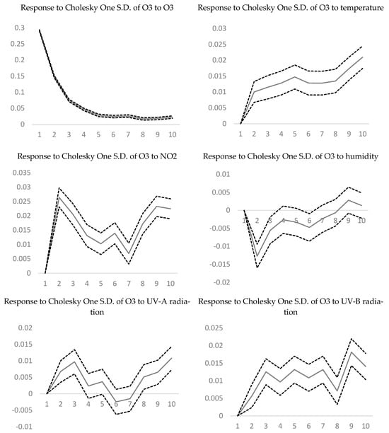
Figure 3.
Impulse responses of the concentration of O3 (solid lines) to one standard deviation (dotted lines) shocks in its precursors. The Cholesky ordering: O3, NO2, Relative humidity, temperature, UV–A radiation, UV–B radiation.
The response of O3 to its own shocks results in a positive decreasing impact during the first 5 days. It also suggests that a one-standard-deviation shock in temperature leads to an increase in ozone concentration during the first five days. That is, temperature has an unambiguous increasing effect on tropospheric O3 in Mexico City, which suggests a nonlinear response.
The impulse response functions also indicate that a one-standard-deviation shock to nitrogen oxides sharply increases the concentration of O3 on the first day, followed by a decrease after the second day, suggesting that reducing nitrogen oxides is necessary to decrease O3 in the medium term.
On the other hand, a relative humidity shock (an increase in relative humidity by one standard deviation) reduces the O3 for 8 days. The response of O3 to UV-A and UV-B shocks is positive. In the first three days, O3 shows an increasing response, followed by a decreasing response.
3.2. Seasonal Behavior
Tropospheric O3 in Mexico City exhibits two seasons of high concentrations, one occurring towards the end of November during the cold, dry season. The other, more intense, happens in April and May during the hot, dry season. Figure 4 illustrates this behavior with the seasonal daily averages of maximum O3 and temperature. The vigorous sunlight intensity, one of the most critical factors affecting and enhancing O3 formation, is usually characterized by relatively high temperatures in April and May. The winter O3 season is characterized by a shallower mixed layer, which promotes the interaction of O3 precursors, allowing them to react more effectively. Additionally, urban environments are sometimes subject to a heat island effect, characterized by high temperatures resulting from the heat released by cars, buildings, and industrial activities, which simultaneously promotes O3 formation [15]. The data was organized in this way because an increase in temperature during the O3 season implies higher concentrations than in a non-O3 season.
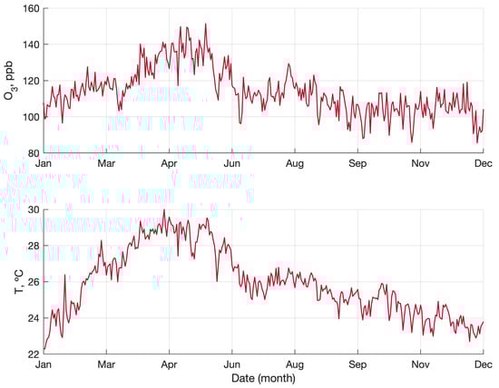
Figure 4.
Seasonal daily average of maximum O3 and temperature (2000–2021).
3.3. Assessing the Relationship Between Ozone and Temperature Using a Nonlinear Model
The link between O3 concentration and surface temperature is complex because its production depends on different variables and their interactions, such as the environmental policy measures, physical parameters (i.e., relative humidity, UV-A and UV-B radiation, etc.), and chemical precursors (i.e., NO, NO2, OH, etc.), whose formation is sometimes dependent on temperature. We assessed the bivariate relationship between such variables in Table 3 and Figure 5. We chose an exponential function due to its theoretical basis when the dependent variable changes at a rate proportional to its current value. The regression model indicates that tropospheric O3 production does not increase linearly with temperature, which accelerates numerous chemical reactions.
Table 3.
Basic statistics of maximum temperature and ozone (2000–2021).
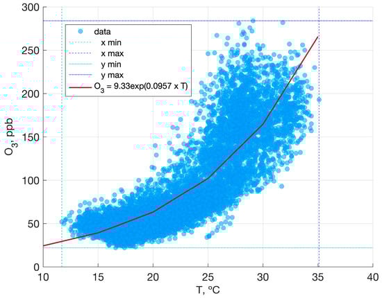
Figure 5.
Maximum O3 concentration versus maximum temperature during 2000–2021.
However, O3 precursor emissions from anthropogenic and biogenic sources are closely related to temperature. Therefore, a statistically significant correlation exists between the variables, although causality cannot be established.
The exponential model outperforms a linear alternative based on ΔAIC = −47 and ΔBIC = −39. Residuals show no significant heteroscedasticity (Breusch–Pagan p = 0.18) and follow approximate normality (Shapiro–Wilk p = 0.21), confirming that the exponential form is appropriate for characterizing sensitivity rather than serving as a deterministic predictive model.
The exponential fit to the data following the equation [O3] = A × exp (b × T), where A and b are the constant and regression coefficients, respectively. O3 concentrations were expressed in parts per billion (ppb), and temperatures in degrees Celsius.
When we used the maximum values of ozone concentration and temperature for the period from 2000 to 2021, the exponential fit was [O3] = 9.33 × exp (0.0957 × T), with a determination coefficient of 0.75 (Figure 5).
The O3 reduction rate has changed over time since 2000, and the association between surface temperature and O3 has varied across different periods. The precursor reduction measures imposed by the Mexico City authorities have modified the concentration of pollutants in the atmosphere and the production of secondary compounds, as indicated by the reduction in the concentration rate, as shown in Table 1. We sorted the daily maximum O3 concentration and maximum temperature for each five-year group. It is worth noting that the relationship between the two variables exhibits an exponential behavior at the disaggregated level (for every five years), as shown in Figure 6. Table 4 shows the main results of the regression adjustments (Supplementary Material Table S2).
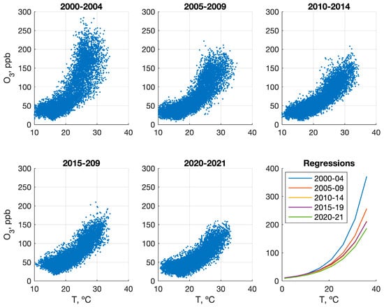
Figure 6.
Maximum O3 concentration versus maximum temperature for each five—year group.
Table 4.
Exponential adjustment coefficients.
The constant A increases for the five-year groups (from 8.431 to 10.280), indicating that O3 starts at a higher value for the minimum temperature. The exception applies to the years 2020–2021, as it was a pandemic event, and atypical behavior was expected.
On the contrary, the slope b decreases for the five-year groups (from 0.1051 to 0.0839). Therefore, the rate of change in ozone for a given temperature change is not constant over the years, which probably implies that policies to reduce precursors were effective over time. Also, there is less variation in maximum O3 concentrations over time. However, the trend follows the exponential form in all cases (Figure 6). The statistical comparison of adjustment coefficients across periods is summarized in Table 4.
4. Discussion
The exponential fit is like the Arrhenius equation, which describes how the rate constant of a chemical reaction depends on temperature. However, ozone production involves a complex series of responses (e.g., NO2 photolysis and VOC oxidation) and other physical parameters (relative humidity, solar radiation, wind speed, etc.). The two terms represent temperature-dependent and temperature-independent parameters.
Given the multivariate nature of ozone formation, R2 values near 0.75 remain meaningful and consistent with similar studies in other megacities [17]. This model quantifies sensitivity of ozone to temperature rather than providing full deterministic prediction.
Although temperature has a significant effect on ozone formation, VAR results (Table 2) indicate that NO2 variability explains a larger portion of ozone response—underscoring the dominant role of precursor availability. Therefore, Therefore, temperature should not be interpreted as the primary driver, but as a modifying factor whose influence intensifies under warming conditions and stagnant meteorology. As indicated by the VAR analysis (Table 2), shocks to NO2 explain a larger fraction of ozone forecast error variance than temperature, underscoring that precursor availability dominates ozone formation. Temperature should therefore be interpreted as an amplifying factor whose influence increases under stagnant and warming conditions, rather than as the dominant cause of extreme ozone episodes.
The pre-exponential coefficient A represents the theoretical ozone concentration at a temperature of 0 °C if the chemical system behaves linearly up to that temperature, which is not the case. A is a term that encompasses variables that are not temperature-dependent and influence the O3 concentration, such as background NOx and VOC concentrations, the strength of the sun, which provides the energy for photolysis reactions, and is partially independent of temperature (e.g., dependent on latitude, season, time of day, and cloudiness), the presence of other compounds that can inhibit or promote O3 formation (e.g., radical sinks), the average boundary layer depth, and the wind patterns that dilute pollutants. A shift in the VOC/NOx ratio toward a more VOC-limited regime (where NOx reductions can increase ozone) is a common occurrence in urban areas as NOx controls take effect [30,31], as is an increase in insufficiently regulated VOC sources or changes in other ozone-forming compounds.
Observed decreases in ambient NO2 levels at RAMA monitoring stations between 2000 and 2021, along with documented reductions in anthropogenic VOC emissions reported in successive ProAire programs, support the observed decline in the sensitivity parameter b. Reduced precursor abundance lowers atmospheric reactivity, mitigating the amplification effect of temperature on ozone formation, consistent with VOC-limited chemical regimes [2,30,31].
The exponent coefficient b encapsulates the temperature-dependent activities that lead to O3 production. Therefore, b is the kinetic force of temperature on the photochemical system. Higher temperatures provide more energy to accelerate the net rate of O3 production. The decrease in the exponential coefficient b over five-year periods (Table 4) indicates that, while the fundamental exponential relationship persists, the sensitivity of O3 formation to temperature has decreased. It is likely a direct consequence of policies aimed at reducing NOx and VOCs, which decrease the atmosphere’s reactivity to the same temperature stimulus. The coefficient b decreases over time (from 0.1051 in 2000–2004 to 0.0839 in 2015–2019) and suggests that O3 production in the atmosphere of Mexico City has declined. The chemical regime and the atmospheric system are now less sensitive to temperature increases than they were two decades ago. Our observation that b decreases over time aligns with studies in Los Angeles and Beijing, where NOx controls initially reduce temperature-driven ozone formation before long-term warming re-enhances it [3,17,32]. Comparable interactions have been projected for Europe under future emissions and climate scenarios [16]. These parallels suggest that while Mexico City’s atmosphere has become less reactive due to policy interventions, continued warming may partially offset mitigation gains [3].
Although A and b are not intended as strict mechanistic partitions of ozone formation pathways, they represent meaningful empirical descriptors. Parameter A aggregates temperature-independent influences such as precursor background concentrations, boundary layer dynamics, and seasonal solar radiation patterns, while parameter b reflects temperature-dependent acceleration of photochemical oxidation. This interpretation is consistent with Arrhenius-type temperature sensitivity in VOC-limited megacities [29,30,32].
5. Conclusions
The exponential model reveals the nonlinear nature of the relationship and captures the increasing risk of high O3 events during heatwaves. As we live in an era of global warming, it is essential to understand the implications of maintaining good air quality and effective climate change management. Based on the relationship between O3 and temperature, it is expected to persist in a warmer future climate.
Therefore, the exponential fit also considers the policy actions and strategies aimed at reducing O3 precursor emissions. Ref. [26] state that the strong correlation between elevated ozone and temperature is a ubiquitous feature in observations in polluted regions. It is consistent with the strong correlation between O3 pollution episodes and temperature in Mexico City (Figure 5 and Figure 6). Air pollution episodes in Mexico City commonly develop in warm, clear, and stagnant conditions associated with dry high-pressure systems. Both meteorological conditions and chemical processes, including precursor emission, influence extreme O3 events. The most extreme events typically occur during heat waves, when abundant radiation facilitates photochemical processes, including temperature-sensitive biogenic and anthropogenic emissions, leading to accumulation in the near-surface air.
Despite the establishment of public policies aimed at reducing O3 concentration, the trend over the years continues with a nonlinear relationship to temperature (Figure 6). Climate change is projected to degrade air quality in polluted regions through adverse modifications in air pollution. Furthermore, future climate change projections for Mexico City predict temperature spikes during the hot and dry seasons, as well as an overall increase in mean temperature. Therefore, a quantitative understanding of how regional air pollution meteorology responds to warming and climate variability could contribute to air quality planning for the coming decades.
Supplementary Materials
The following supporting information can be downloaded at: https://www.mdpi.com/article/10.3390/atmos16121379/s1, Table S1: RAMA and REDMET instrumentation, Figure S1: Exponential adjustment of O3 maxima and temperature grouped by 10-year (2000–2009 and 2010–2021); Figure S2: Maxima NO2 daily concentrations (gray dots) and 30-day moving average (blue line); Table S2: Exponential adjustment of O3 maxima and temperature grouped by 10-year (2000–2009 and 2010–2021).
Author Contributions
T.C.: Conceptualization and investigation; A.S.-V.: formal analysis and computing resources; A.S.: software, validation, data curation, methodology; O.P.: writing, visualization, methodology. All authors have read and agreed to the published version of the manuscript.
Funding
This research received no external fundings.
Institutional Review Board Statement
Not applicable.
Informed Consent Statement
Not applicable.
Data Availability Statement
All data used by the author is publicly available at RAMA web portal at https://www.aire.cdmx.gob.mx/default.php (accessed on 1 September 2025).
Acknowledgments
The authors would like to thank Isabel Saavedra from Instituto de Ciencias de la Atmósfera y Cambio Climático, UNAM, their help reviewing the article; and Lizeth Guerrero González from Instituto de Investigaciones Economicas; UNAM, for her help on econometric calculations.
Conflicts of Interest
The authors declare no conflicts of interest.
References
- Crutzen, P.J.; Lawrence, M.G.; Pöschl, U. On the background photochemistry of tropospheric ozone. Tellus B Chem. Phys. Meteorol. 1999, 51, 123–146. [Google Scholar] [CrossRef]
- Sillman, S.; Samson, P.J. Impact of temperature on oxidant photochemistry in urban, polluted rural and remote environments. J. Geophys. Res. Atmos. 1995, 100, 11. [Google Scholar] [CrossRef]
- Steiner, A.L.; Davis, A.J.; Sillman, S.; Owen, R.C.; Michalak, A.M.; Fiore, A.M. Observed suppression of ozone formation at extremely high temperatures due to chemical and biophysical feedbacks. Proc. Natl. Acad. Sci. USA 2010, 107, 19685–19690. [Google Scholar] [CrossRef] [PubMed]
- EPA. Trends in Ozone Adjusted for Weather Conditions. 2020. Available online: https://www.epa.gov/air-trends/trends-ozone-adjusted-weather-conditions#:~:text=Ozone%20is%20more%20readily%20formed,cool%2C%20rainy%2C%20or%20windy (accessed on 1 September 2025).
- Jacob, D.J.; Winner, D.A. Effect of climate change on air quality. Atmos. Environ. 2009, 43, 51–63. [Google Scholar] [CrossRef]
- Dear, K.; Ranmuthugala, G.; Kjellström, T.; Skinner, C.; Hanigan, I. Effects of Temperature and Ozone on Daily Mortality During the August 2003 Heat Wave in France. Arch. Environ. Occup. Health 2005, 60, 205–212. [Google Scholar] [CrossRef]
- Peel, J.L.; Haeuber, R.; Garcia, V.; Russell, A.G.; Neas, L. Impact of nitrogen and climate change interactions on ambient air pollution and human health. Biogeochemistry 2013, 114, 121–134. [Google Scholar] [CrossRef]
- Crutzen, P.J. The influence of Nitrogen Oxides on Atmospheric Ozone Content. In Paul J. Crutzen: A Pioneer on Atmospheric Chemistry and Climate Change in the Anthropocene; Springer: Cham, Switzerland, 2016; pp. 108–116. [Google Scholar] [CrossRef]
- Townsend, A.R.; Howarth, R.W.; Bazzaz, F.A.; Booth, M.S.; Cleveland, C.C.; Collinge, S.K.; Dobson, A.P.; Epstein, P.R.; Holland, E.A.; Keeney, D.R.; et al. Human health effects of a changing global nitrogen cycle. Front. Ecol. Environ. 2003, 1, 240–246. [Google Scholar] [CrossRef]
- Brewer, A.W.; McElroy, C.T.; Kerr, J.B. Nitrogen dioxide concentrations in the atmosphere. Nature 1973, 246, 129–133. [Google Scholar] [CrossRef]
- Ravishankara, A.R.; Daniel, J.S.; Portmann, R.W. Nitrous oxide (N2O): The dominant ozone-depleting substance emitted in the 21st century. Science 2009, 326, 123–125. [Google Scholar] [CrossRef]
- Weber, B.; Wu, D.; Tamm, A.; Ruckteschler, N.; Rodríguez-Caballero, E.; Steinkamp, J.; Meusel, H.; Elbert, W.; Behrendt, T.; Sörgel, M.; et al. Biological soil crusts accelerate the nitrogen cycle through large NO and HONO emissions in drylands. Proc. Natl. Acad. Sci. USA 2015, 112, 15384–15389. [Google Scholar] [CrossRef]
- Kinnison, D.; Johnston, H.; Wuebbles, D. Ozone calculations with large nitrous oxide and chlorine changes. J. Geophys. Res. Atmos. 1988, 93, 14165–14175. [Google Scholar] [CrossRef]
- Molina, L. Introductory lecture: Air quality in megacities. Faraday Discu. 2021, 226, 9–52. [Google Scholar] [CrossRef]
- Stathopoulou, E.; Mihalakakou, G.; Santamouris, M.; Bagiorgas, H.S. On the impact of temperature on tropospheric ozone concentration levels in urban environments. J. Earth Syst. Sci. 2008, 117, 227–236. [Google Scholar] [CrossRef]
- Nolte, C.G.; Spero, T.L.; Bowden, J.H.; Sarofim, M.C.; Martinich, J.; Mallard, M.S. Regional temperature-ozone relationships across the U.S. under multiple climate and emissions scenarios. J. Air Waste Manag. Assoc. 2021, 71, 1251–1264. [Google Scholar] [CrossRef] [PubMed]
- Petres, S.; Lanyi, S.; Pirianu, M.; Keresztesi, A.; Nechifor, A.C. Evolution of Tropospheric Ozone and Relationship with Temperature and NOx for the 2007–2016 Decade in the Ciuc Depression. Rev. Chim. 2018, 69, 602–608. [Google Scholar] [CrossRef]
- Estrada, F.; Zavala, J.; Martínez, A.; Raga, G.; Gay, C. State and Perspectives of Climate Change in Mexico a Starting Point; UNAM Climate Change Research Program: Mexico City, Mexico, 2023; ISBN 978-607-30-8172-6. Available online: https://cambioclimatico.unam.mx/wp-content/uploads/2023/12/State-and-Perspectives-of-Climate-Change-in-Mexico-a-Starting-Point.pdf (accessed on 1 September 2025).
- ProAire. Programa Para Mejorar la Calidad Del Aire en la Zona Metropolitana Del Valle De México 2011–2020; Anexo 8; Secretaría de Medio Ambiente: Mexico City, Mexico, 2020. Available online: https://www.aire.cdmx.gob.mx/descargas/publicaciones/flippingbook/proaire-2011-2020-anexos/ (accessed on 1 September 2025).
- EPA. A Guide to the UV Index; United States Environmental Protection Agency: Washington, DC, USA, 2004. Available online: https://www.epa.gov/sites/default/files/documents/uviguide.pdf (accessed on 1 September 2025).
- Andrady, A.; Aucamp, P.J.; Bais, A.F.; Ballare, C.L.; Björn, L.O.; Bornman, J.F.; Caldwell, M.; Cullen, A.P.; Erickson, D.J.; Häder, D.P.; et al. Environmental effects of ozone depletion and its interactions with climate change: Progress report, 2009. Photochem. Photobiol. Sci. 2010, 9, 275–294. [Google Scholar] [CrossRef]
- Barnes, P.W.; Robson, T.M.; Neale, P.J.; Williamson, C.E.; Zepp, R.G.; Madronich, S.; Wilson, S.R.; Andrady, A.L.; Heikkilä, A.M.; Bernhard, G.H.; et al. Environmental effects of stratospheric ozone depletion, UV radiation, and interactions with climate change: UNEP Environmental Effects Assessment Panel, Update 2021. Photochem. Photobiol. Sci. 2022, 21, 275–301. [Google Scholar] [CrossRef]
- Ayité-Lo, N.A.; Albriton, D.L.; Watson, R.T. Scientific Assessment of Ozone Depletion: 2006; World Meteorological Organization: Geneva, Switzerland, 2006. [Google Scholar]
- Norval, M.; Cullen, A.P.; De Gruijl, F.R.; Longstreth, J.; Takizawa, Y.; Lucas, R.M.; Noonan, F.P.; Van der Leun, J.C. The effects on human health from stratospheric ozone depletion and its interactions with climate change. Photochem. Photobiol. Sci. 2007, 6, 232–251. [Google Scholar] [CrossRef] [PubMed]
- Valuntaitė, V.; Šerevičienė, V.; Girgždienė, R.; Paliulis, D. Relative humidity and temperature impact to ozone and nitrogen oxides removal rate in the experimental chamber. J. Environ. Eng. Landsc. Manag. 2012, 20, 35–41. [Google Scholar] [CrossRef]
- Wise, E.K.; Comrie, A.C. Extending the Kolmogorov-Zurbenko Filter: Application to Ozone, Particulate Matter, and Meteorological Trends. J. Air Waste Manag. Assoc. 2005, 55, 1208–1216. [Google Scholar] [CrossRef]
- Sims, C.A. Macroeconomics and Reality. Econometrica 1980, 48, 1–48. [Google Scholar] [CrossRef]
- Stock, H.J.; Watson, M.W. Vector Autoregressions. J. Econ. Perspect. 2001, 15, 101–115. [Google Scholar] [CrossRef]
- Sanchez, A.; Mansilla, R.; Aguilar, A. An Empirical Analysis of the Nonlinear Relationship Between Environmental Regulation and Manufacturing Productivity. J. Appl. Econ. 2013, 16, 357–372. [Google Scholar] [CrossRef]
- Torres-Jardón, R.; García-Reynoso, J. Assessment of the ozone-nitrogen oxide-volatile organic compound sensitivity of Mexico City through an indicator-based approach: Measurements and numerical simulations comparison. J. Air Waste Manag. Assoc. 2009, 59, 1155–1172. [Google Scholar] [CrossRef]
- Peralta, O.; Ortínez-Alvarez, A.; Torres-Jardón, R.; Suárez-Lastra, M.; Castro, T.; Ruíz-Suárez, L.G. Ozone over Mexico City during the COVID-19 pandemic. Sci. Total Environ. 2021, 761, 143183. [Google Scholar] [CrossRef] [PubMed]
- Aucamp, P.J.; Björn, L.O.; Lucas, R. Questions and answers about the environmental effects of ozone depletion and its interactions with climate change: 2010 assessment. Photochem. Photobiol. Sci. 2011, 10, 301–316. [Google Scholar] [CrossRef] [PubMed]
Disclaimer/Publisher’s Note: The statements, opinions and data contained in all publications are solely those of the individual author(s) and contributor(s) and not of MDPI and/or the editor(s). MDPI and/or the editor(s) disclaim responsibility for any injury to people or property resulting from any ideas, methods, instructions or products referred to in the content. |
© 2025 by the authors. Licensee MDPI, Basel, Switzerland. This article is an open access article distributed under the terms and conditions of the Creative Commons Attribution (CC BY) license (https://creativecommons.org/licenses/by/4.0/).