Abstract
Extreme heat across the North Indian Plain has intensified in recent decades, with the temperature in Delhi repeatedly exceeding 48 °C. We present a physically interpretable and computationally efficient typology of heatwave risk using aggregated station observations of daily mean temperature, relative humidity, wind speed, and pressure from 1997 to 2016. Quality-controlled, standardized daily features (PCA-verified) were clustered with k-means; internal validity indices (Silhouette, Calinski–Harabasz, and Davies–Bouldin) identified an optimal partition with k = 3, defining three distinct weather regimes. Coupling these regimes with an absolute heatwave criterion (daily mean ≥30 °C for ≥3 days) revealed a pronounced gradient: a dry–hot, high-pressure regime (41% of days) accounted for 63% of heatwave days (mean 33.4 °C; median duration ≈17 days); a mild–humid background (59%) yielded ~8% incidence; and a rare blocking-driven dry intrusion (<1%) produced heatwaves each time, with mean temperatures of >35 °C and episodes persisting for ≥30 days. Regime–heatwave relationships were statistically significant and robust across sensitivity tests, including variations in k, alternative clustering algorithms, and bootstrap resampling. This four-stage workflow consists of data preparation, feature extraction, regime classification, and heatwave risk attribution and provides a transparent basis for regime-aware early warning, demand-side energy management, and public health protection in Delhi and is transferable to other rapidly urbanizing regions.
1. Introduction
Heatwaves are commonly defined as sustained periods of abnormally high temperatures in a given region and constitute a typical extreme temperature phenomenon [,]. As a compound hazard, they exert wide-ranging and profound impacts on human health [], ecosystems [], and critical infrastructure [,], with several reviews documenting the breadth of consequences []. Over recent decades, the frequency and severity of extreme weather events, including heatwaves, have generally increased, consistent with signals of global climate change [,,]. The latest IPCC assessment further indicates that urban populations will face substantially higher exposure to dangerous heat and humidity over this century []. Complementing this outlook, projections under high-emissions scenarios and assuming no adaptation suggest that by 2100, extreme heat could result in approximately 5.1 million additional hospitalizations [].
A growing body of evidence shows that heatwave impacts are especially pronounced in India and exhibit strong spatial heterogeneity. Socio-environmental vulnerability is highest across several central and eastern states where persistent poverty and limited public services prevail [], while risk is rising in the mid-elevation Himalaya (1000–2000 m) due to high population density and agricultural dependence []. Within cities, informal settlements and poorly ventilated aging buildings are particularly sensitive to heatwaves and pluvial flooding, and equity concerns are often under-addressed in adaptation planning []. Economic assessments estimate that intensifying heat exposure alone could push ~50 million people in India back into poverty by 2040 []. For the Delhi–Ganges Plain, projections indicate >30 lethal heat–humidity days per year by the 2050s, increasing to >60 days by 2100 if high-emission conditions persist [,].
Despite these substantial impacts, there is no single, standardized definition of a heatwave: intensity, spatial extent, and duration vary by location, and precise criteria remain unsettled [,]. A temperature considered moderate in one region may be perceived as hot in another. The World Meteorological Organization has not promulgated a comprehensive, universally applicable definition because heatwaves differ in their characteristics and severity []. In light of regional climatic and socio-adaptive differences, this study adopts, for Delhi, an absolute threshold as the primary criterion: daily mean temperature ≥ 30 °C for ≥3 consecutive days. This choice aligns operationally with the India Meteorological Department (IMD) practice that emphasizes absolute Tmax thresholds combined with anomaly based rules []. To ensure cross-study comparability, we conducted parallel percentile-based sensitivity tests (P90–P95) []. Relative to definitions based solely on Tmax, the daily mean temperature better reflects limited nocturnal cooling and cumulative heat exposure: nighttime heatwaves commonly arise from insufficient nocturnal radiative cooling and sustained heat accumulation, and multi-country evidence links cumulative heat load directly to health risks, including excess mortality [,,].
In data-driven frameworks, unsupervised clustering—particularly K-means—is widely used to extract heatwave “regimes” or homogeneous temperature-field regions. National-scale studies show that K-means, in large-sample, low-noise settings, more efficiently pinpoints heat hotspots than MiSTIC []. At the urban scale, K-means/Fuzzy C-means is often combined with Innovative Trend Analysis (ITA) and Mann–Kendall tests to characterize homogeneous regions of Delhi’s rainfall and heatwaves and their long-term trends []. In dynamic-forecasting research, TIGGE and WRF studies also employ K-means to classify 500 hPa blocking clusters in order to explain ≥5-day heatwave forecast errors and improve ensemble weighting []. However, K-means applications often face two generic issues: (i) the cluster number k is chosen subjectively, leading to potentially unstable solutions [,], and (ii) relying solely on internal validity indices may not guarantee external physical relevance [].
To address these limitations, we aggregate hourly station observations to daily features—temperature, relative humidity, wind speed, and surface pressure—and then apply K-means with k = 3. Methodologically, we (a) represent the city-scale daily weather state with the four standardized features to preserve signals often attenuated in coarse-grid products; (b) determine the optimal k using a joint model-selection approach with the Silhouette, Calinski–Harabasz, and Davies–Bouldin indices; and (c) evaluate robustness via algorithmic substitution (Gaussian mixture models and hierarchical clustering) and 100 bootstrap resamples, quantified with the adjusted Rand index (ARI > 0.90). Finally, we anchor the resulting cluster centroids and regimes to physical diagnostics of blocking highs and soil moisture deficits, thereby building a bridge between statistical grouping and dynamical interpretation.
The main questions posed in this study are how to objectively determine the number of heatwave regimes in Delhi and how to ensure that clustering results are physically interpretable rather than purely statistical. We address these by developing a four-step framework: aggregating multi-variable daily weather features, applying K-means clustering with multiple model-selection indices, testing robustness through alternative algorithms and bootstrap resampling, and linking the resulting regimes to physical processes such as blocking highs and soil moisture deficits. This approach provides a computationally efficient and transferable tool for regime-aware early warning, energy management, and public health protection in Delhi and other rapidly urbanizing regions.
Distinct from previous studies, this work advances heatwave risk classification in several ways. First, it introduces a multi-metric optimization of K-means clustering (Silhouette, Calinski–Harabasz, Davies–Bouldin, SSE) to avoid the subjective selection of cluster numbers common in earlier analyses. Second, it explicitly anchors statistical clusters to physical drivers such as subtropical ridges, blocking highs, and soil moisture deficits, enhancing the dynamical interpretability of the results. Third, it provides one of the first long-term, station-based validations for Delhi (1997–2016) with robust testing through bootstrap resampling and alternative clustering algorithms. Finally, it integrates regime-aware heatwave risk typing with operationally relevant absolute temperature thresholds, offering a transparent and transferable workflow for early warning, demand-side energy management, and public health protection in heat-vulnerable cities.
2. Materials and Methods
2.1. Data Sources and Preprocessing
Our analysis is based on hourly weather observations from 1997 to 2016, openly sourced from the “Delhi Weather Data” dataset available on Kaggle (provided by Mahir Kukreja) (https://www.kaggle.com/datasets/mahirkukreja/delhi-weather-data, accessed on 7 July 2025). Our analysis focuses on the National Capital Territory (NCT) of Delhi, India (approximately 28.4–28.9° N, 76.8–77.4° E), located in the northwestern Indo-Gangetic Plain. Figure 1 shows the location of the study area within India and the administrative area of Delhi used for analysis.
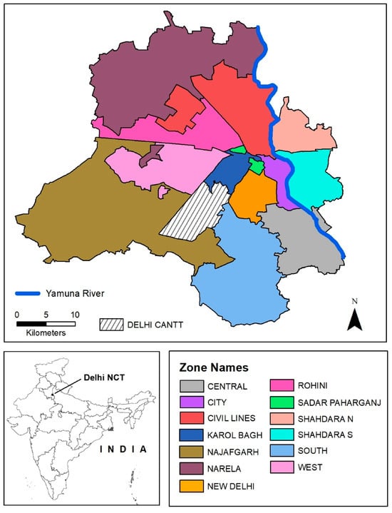
Figure 1.
Location of the study area: the National Capital Territory (NCT) of Delhi (28.4–28.9° N, 76.8–77.4° E), India. Base map adapted from Mitchell et al. (2021) [], Social Inequities in Urban Heat and Greenspace: Analyzing Climate Justice in Delhi, India.
The original dataset comprises 98,292 records across 20 meteorological variables. Based on their relevance to thermodynamic, moisture, and dynamic processes, six key variables were selected for heatwave analysis: temperature, relative humidity, wind speed, pressure, dew point temperature, and visibility (Table 1). Precipitation was excluded due to extensive missing data, and other secondary variables were omitted to reduce redundancy.

Table 1.
Core meteorological variables used for heatwave analysis.
Missing values in the selected variables accounted for less than 5% of the total records (Figure 2). Short gaps (<6 h) were filled via linear interpolation, while longer gaps (≥6 h) were imputed using the multi-year daily mean for the corresponding calendar day. The hourly data were then aggregated into daily summary variables: maximum (T_max), minimum (T_min), and mean temperature (T_mean); mean relative humidity (H_mean); mean wind speed (W_mean); and mean pressure (P_mean). These derived metrics form a consistent and interpretable basis for subsequent clustering and statistical modeling.
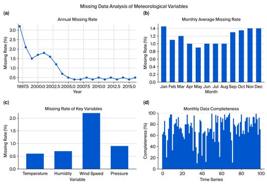
Figure 2.
Missing data diagnostics (1997–2016): (a) annual missing rate; (b) monthly mean missing rate; (c) missing rate by variable; (d) monthly data completeness time series. The panels collectively show that core variables have low and declining missing rates, and that data quality meets the requirements for subsequent analyses. Note: Panels (b,d) reflect aggregate monthly averages across the retained key variables (temperature, humidity, wind speed, and pressure), rather than individual variable series.
Figure 3 presents the sequential analytical procedure adopted in this study. The process begins with data preparation, including quality control, hybrid gap-filling, and daily aggregation of the key variables (T_mean, H_mean, W_mean, and P_mean). This is followed by feature extraction, where variable screening, Z-score normalization, and principal component analysis (PCA) are applied. Next, regime classification is performed using K-means clustering (k = 3), validated by multiple diagnostic indices and supported by diagnostic visualization. Finally, heatwave risk attribution links the identified regimes with heatwave definitions and conducts statistical testing (χ2 and ANOVA), along with robustness assessments such as sensitivity to k, bootstrap resampling, and algorithm comparison.
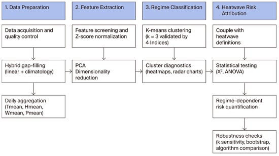
Figure 3.
Analytical Workflow of the Study.
2.2. Weather-Regime Clustering Method
2.2.1. Feature Selection and Standardization
Based on heatwave generation theory and the results of correlation analysis, the Pearson correlation matrix (Figure 4a) shows that all pairwise correlation coefficients lie between −0.466 and 0.274, indicating no significant multicollinearity. To eliminate the influence of differing units, all features were standardized using Z-score normalization:
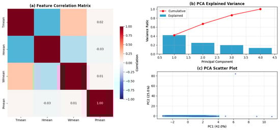
Figure 4.
Feature Correlation Matrix (a) and PCA variance explained (b), scatter plot (c).
Here, X denotes the original feature value, and μ and σ are its sample mean and standard deviation values, respectively.
2.2.2. Principal Component Analysis (PCA)
The correlation matrix reveals a moderate negative correlation between T_mean and H_mean (r = −0.47), and a weak positive correlation between T_mean and W_mean (r = 0.27). Pmean is nearly independent of the other three variables (|r| ≤ 0.03). An unconstrained PCA was then applied to the standardized matrix (Figure 4b,c): the first and second principal components (PC1 and PC2) explain 42% and 25% of the variance, respectively, with a cumulative contribution of 67%, exceeding the 60% threshold for information retention. Samples mainly spread along PC1, while PC2 provides secondary orthogonal separation, demonstrating that the first two principal components can effectively capture the sample variability.
2.2.3. Cluster Results and Interpretation
After determining the principal components, we applied K-means clustering in the (PC1, PC2) subspace and systematically searched for the optimal number of clusters k based on four internal validity indices: Silhouette, Calinski–Harabasz, Davies–Bouldin, and SSE (Elbow). This strategy balances within-cluster compactness and between-cluster separation while avoiding model overfitting.
The combined response of the four indices is summarized in Figure 5. The Calinski–Harabasz index reaches its maximum at k = 3, and the Elbow curve also exhibits a clear inflection around k ≈ 3–4. Although the Davies–Bouldin index attains its lowest value at k = 2, its value at k = 3 remains close to that minimum and improves markedly compared with higher k. At the same time, the Silhouette score decreases slightly from k = 2 to k = 3 but remains relatively stable afterward. Considering the overall balance among the four indices and the interpretability of the clusters, k = 3 is selected as the optimal compromise for subsequent analyses.

Figure 5.
Determination of optimal k using four indices.
The characteristics of the cluster structure are summarized in Figure 6. The heat map (Figure 6a) shows that Cluster 0 is marked by pronounced positive departures in T_mean and W_mean together with a slight negative anomaly in P_mean, typifying the hot–dry–low-pressure Regime I. Cluster 1 exhibits lower temperature, higher humidity, and near-normal pressure, matching the mild–humid Regime II. Cluster 2 combines the highest temperatures, the lowest humidity, and the deepest pressure deficit, representing the blocking-induced dry-intrusion Regime III. Figure 6b (radar plot) shows the standardized four-variable spectra, which clearly delineate the physical boundaries among the three clusters and provide a robust typological framework for subsequent heatwave risk attribution and tiered early-warning design.
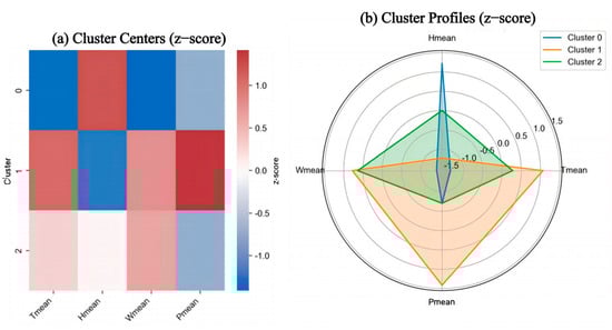
Figure 6.
Cluster center heatmap and radar profiles.
2.3. Heatwave Risk Assessment Based on Weather Regimes
2.3.1. Heatwave Threshold Determination
A two-path sensitivity test was performed (Figure 7a–c). Scanning absolute thresholds (24–36 °C) showed an exponential decay of hot-day samples, with 30 °C balancing sample size and event intensity (Figure 7a). Applying T_mean ≥ 30 °C for ≥3 days reproduced midsummer peaks and excluded moderate warming (Figure 7b). Percentile scans (85th–99th, ≈32–38 °C) revealed a sharp decline in events from 113 to 5 as thresholds rose (Figure 7c). Considering comparability and regional applicability, both absolute (30 °C, ≥3 days) and percentile (90th–95th) thresholds were retained for subsequent analysis.
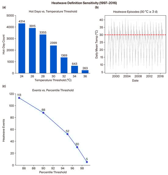
Figure 7.
Comparison of heatwave definitions in Delhi (1997–2016). (a) Total number of hot days under different absolute temperature thresholds (24–36 °C), showing how increasing thresholds sharply reduce hot-day counts. (b) Time series of daily mean temperature with the 30 °C threshold (≥3 consecutive days) illustrating identified heatwave episodes. (c) Number of heatwave events under different percentile-based thresholds (86th–98th), demonstrating the sensitivity of event detection to relative definitions.
2.3.2. Regime-Based Risk Attribution
Daily data were paired with the heatwave criterion (Tₘₑₐₙ ≥ 30 °C for ≥3 days) to evaluate regime-specific risks (Figure 8). Cluster 0 (warm–dry, 41% of samples) contributes 63% of heatwave days and dominates regional risk. Cluster 1 (mild–humid) shows only ~8% incidence, forming a low-risk background. Cluster 2 (extreme anomaly) is rare but exhibits 100% incidence, representing a high-impact tail. Seasonal curves (Figure 8b) highlight Cluster 0’s persistence into early autumn, while radar charts (Figure 8c) confirm its “hot–dry–variable” danger profile. Overall, Cluster 0 requires primary monitoring, whereas Cluster 2, though infrequent, warrants contingency preparedness.
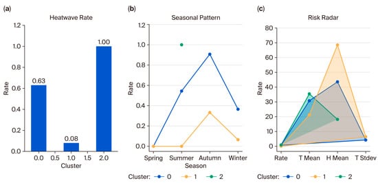
Figure 8.
Heatwave risk assessment based on weather regimes. (a) Heatwave rate across clusters, showing substantial variation in occurrence frequency among the three regimes. (b) Seasonal patterns of heatwave occurrence for each cluster, highlighting dominant seasons of risk. (c) Risk radar comparing key contributing factors (heatwave rate, mean temperature, mean humidity, and temperature variability) across clusters.
2.3.3. Statistical Testing of Regime Dependence
To quantify the dependence between weather regimes and heatwave occurrence, a 3 × 2 contingency table was constructed and a χ2 test was performed (χ2 = 2447.8, p < 0.001), confirming a strong association. One-way ANOVA was applied to the heatwave incidence rate and the four core meteorological variables, each yielding p < 0.001. These results indicate highly significant differences among the three regimes in both heatwave frequency and thermodynamic–moisture–dynamic conditions, providing strong statistical support for a regime-based classification of heatwave risk (see Table 2).
Table 2.
Statistical analysis of heatwave regimes.
2.3.4. Seasonal–Interannual Climatology
The 1997–2016 daily records were reorganized into month–year grids to assess seasonal and interannual patterns (Figure 9). Incidence rises sharply from April, peaks at ~80% in May–June, and gradually declines through September (Figure 9a). Heat maps (Figure 9b) confirm persistent May–August dominance, with near-100% years (e.g., 2009, 2011, 2015). Boxplots (Figure 9c) show stable high summer risk but wide variability in July–August and extended tails in April/September. Overall, Delhi’s heatwave climatology follows an “early onset–summer plateau–long tail” structure, requiring alerts from late April and flexible thresholds in the shoulder seasons.
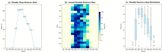
Figure 9.
Monthly heatwave climatology.
2.4. Robustness and Sensitivity Testing of the Clustering
The stability of the three-cluster solution was assessed through variations in K (2–4), internal validation indices, bootstrap resampling, and alternative algorithms (Appendix A Table A1 and Table A2; Figure A1, Figure A2 and Figure A3). Across all K values, the warm–dry, mild–humid, and extreme-anomaly regimes were consistently reproduced, with heatwave incidence rates remaining ~63% in the high-risk cluster, <10% in the low-risk cluster, and 100% in the extreme cluster. Internal indices indicated an optimum at K ≈ 3, while 100 bootstrap replicates yielded ARI values largely > 0.9, with instability only when the extreme cluster was absent. Gaussian mixture and hierarchical clustering produced comparable risk metrics. These results confirm that the three-regime structure is both statistically robust and physically interpretable.
3. Results
3.1. Weather Regime Identification
Using 7161 daily samples of normalized (Z-score) T_mean, H_mean, W_mean, and P_mean (1997–2016), we applied K-means clustering across K = 2–10. All three internal validity indices (Silhouette, Calinski–Harabasz, Davies–Bouldin) peaked at K = 3, confirming this as the optimal cluster solution. Separability was verified in PC1–PC2 subspace prior to clustering. The resulting three weather regimes (Regime I–III) account for 41%, 59%, and ≪1% of the samples, forming the midsummer dry-heat, year-round background, and rare extreme anomaly physical spectra. Figure 10’s four subplots correspond to (a) temperature, (b) humidity, (c) wind speed, and (d) pressure, with bar colors matching the cluster labels and values annotated atop each bar to facilitate intuitive comparison of thermodynamic–moisture–dynamic differences. Regimes I and III together constitute the midsummer dry-heat and extreme-transition ends of the spectrum, while Regime II serves as the persistent background. Cluster centers show that Regime I (Cluster 0) is a typical high-temperature, low-humidity type with T ≈ 29.6 °C, RH ≈ 43.6%, W ≈ 6.1 km h−1, P ≈ 1001 hPa; Regime II (Cluster 1) is a mild–humid type with T ≈ 18.0 °C, RH ≈ 70.2%, W ≈ 5.2 km h−1, P ≈ 1015 hPa; Regime III (Cluster 2) is an extreme anomaly type with T ≈ 31.6 °C, RH ≈ 37.6%, W ≈ 10.2 km h−1, P ≈ 1003 hPa.
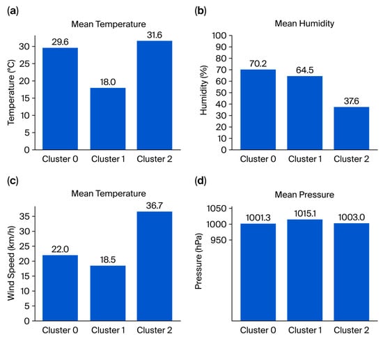
Figure 10.
Cluster-center comparison of core meteorological variables. (a) Mean temperature for each cluster, showing the highest thermal conditions in Cluster 2 and the lowest in Cluster 1. (b) Mean humidity across clusters, indicating a sharp decrease from Cluster 0 to Cluster 2. (c) Mean wind speed, highlighting stronger winds associated with Cluster 2 compared to other regimes. (d) Mean pressure distribution, with Cluster 1 exhibiting slightly higher pressure than the other clusters.
Simultaneously, the interannual line plot in Figure 11a shows that Regime II remains the dominant regime (200–260 d.a−1). Regime I is most frequent around the early 2000s, particularly circa 2005 ± 2 years, and Regime III is exceedingly rare throughout the year. The monthly stacked-area chart in Figure 11b further reveals that Regime I occurs almost exclusively in June–September (peaking in July–August). Regime II is distributed relatively evenly across all seasons, with Regime II slightly supplanted by Regime I during midsummer. Regime III appears only sporadically at the start and end of summer for very brief durations. The transition matrix constructed from the daily sequence (Appendix A Figure A4) indicates that each regime has a self-persistence probability greater than 84%, with transitions occurring mainly between Regime I and Regime II (≈15%), while Regime III almost never transitions to other regimes—demonstrating strong short-term persistence and limited exchange pathways. These statistical characteristics provide temporal constraints and physical context for subsequent regime-based heatwave risk forecasting.
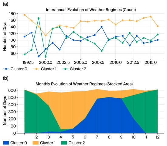
Figure 11.
Temporal evolution of weather regimes. (a) Interannual variation in the number of days for each cluster, illustrating long-term fluctuations and persistence of dominant regimes over the study period. (b) Monthly distribution of weather regimes (stacked area chart), showing the seasonal transition and relative dominance of clusters throughout the calendar year.
3.2. Heatwave Risk Typing and Statistical Tests
3.2.1. Overall Seasonal Distribution of Heatwaves
Based on the 1997–2016 daily mean temperature time series, we first applied the absolute threshold method (“T_mean ≥ 30 °C sustained for ≥3 days”) to identify heatwave events, yielding a total of 1632 heatwave days, averaging about 6.8 days per month over the 20-year (1997–2016, 240 months) period, and then tabulated their monthly distribution characteristics (Figure 12a,b). The bar chart (Figure 12a, with the vertical axis representing heatwave rate) shows that heatwaves are concentrated in May–September: the average incidence rates are highest in May and June, at 85.0% and 81.8%, respectively; July and August also exceed 50%; and heatwaves are virtually absent after October. The jitter plot (Figure 12b) clearly confirms that summer heatwave days form a dense band along the ‘1’ line, while winter months show almost no red points along the ‘0’ line. This reveals a characteristic rhythm of “early onset, summer plateau, and rapid autumn decay” for heatwave risk in this region, which aligns with the typical monsoon-influenced climate of the area, where the warm and moist summer monsoon fosters conditions favorable for heatwave formation.
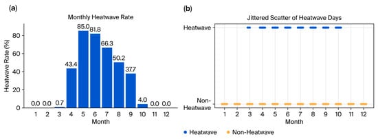
Figure 12.
Monthly heatwave distribution, 1997–2016 ((a) bar chart of incidence rates; (b) jitter plot of daily events).
3.2.2. Heatwave Risk Under Different Weather Regimes
Under the three regimes identified by K-means clustering (K = 3; Section 2.2), distinct risk patterns emerge (Figure 13). Regime I (high-temperature, low-humidity) accounts for 41% of samples but concentrates 63% of all heatwave days. Heatwaves within this regime reach average temperatures of 33.4 °C, persist for nearly 17 days, and occur under relatively dry conditions (mean humidity 42.3%), forming a profile of “hot, dry, and long-lasting” extreme risk. Regime II (mild–humid) covers 59% of samples but contributes only 8% of heatwave days; its events exhibit significantly lower intensity and duration, with high humidity (69.7%) providing partial mitigation of heat stress. Regime III (extreme anomaly) was observed only once during 1997–2016, yet its combination of ≥35 °C temperatures and exceptionally low humidity (18.3%) produced a 100% hit rate, representing sudden-onset, high-severity extremes.
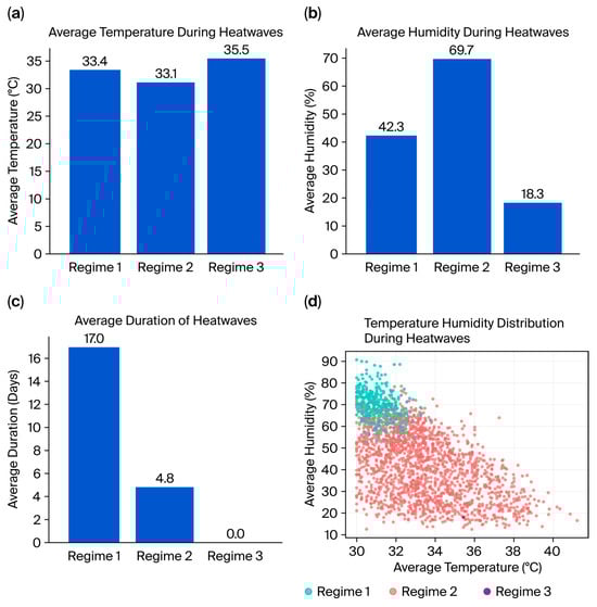
Figure 13.
Heatwave intensity across weather regimes. (a) Average temperature during heatwaves for each regime, indicating the highest thermal intensity under Regime 3. (b) Average humidity during heatwaves, showing markedly higher moisture in Regime 2 and much drier conditions in Regime 3. (c) Average duration of heatwaves, with Regime 1 associated with the longest-lasting events. (d) Joint distribution of temperature and humidity during heatwaves, illustrating the distinct thermodynamic profiles of the three regimes.
The statistical basis of these distinctions was established in Section 2.3.3: a χ2 test confirmed a highly significant association between regimes and heatwave occurrence (χ2 = 2447.8, p < 0.001), and one-way ANOVA indicated significant differences across temperature and other core meteorological variables (all p < 0.001; Table 2). Together, these results demonstrate that the regime-based classification captures physically distinct and statistically robust heatwave risk structures, thereby supporting its application in differentiated warning and mitigation strategies.
3.3. Internal Structure of Heatwave Events
To characterize the internal structure of heatwave events under different weather regimes, we represent each event as a two-dimensional vector of “mean event temperature–duration in days,” colored by its dominant regime (Figure 14a). The results show that Regime I (hot–dry, red) dominates the sample; its point cloud is mainly clustered around 30–34 °C and 3–15 days, but also includes occasional longer events (up to 32 days), indicating that the typical dry-heat background not only triggers frequent heatwaves but can also produce medium to long-duration episodes. Regime III (extreme, cyan), although rare, corresponds to both higher temperatures and longer durations; some events exceed 35 °C and last ≥ 50 days, representing the “low-frequency, high-intensity” extreme end of the spectrum. Together, these two regimes drive the most severe summer heat exposures, with the extreme-anomaly regime contributing disproportionately to the highest-intensity events.
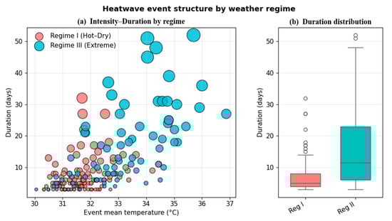
Figure 14.
Structure of heatwave events by weather regime. (a) Intensity–duration distribution of heatwave events, showing the relationship between event mean temperature and duration for Regime I (Hot–Dry) and Regime III (Extreme), with marker size indicating event magnitude. (b) Boxplot of heatwave duration across regimes, highlighting the substantially longer and more variable durations associated with Regime III compared to Regime I.
Figure 14b compares the duration distributions of Regime I and Regime III. Regime I has an interquartile range of 4–8 days and a median of 5 days; Regime III’s IQR expands to 7–23 days with a median of 11 days, and includes a long tail of ≥40 days. A Mann–Whitney U test yields p < 0.001, indicating a significant difference in duration between the two regimes. These results suggest that dry-heat-regime heatwaves occur frequently and follow a fairly consistent pattern, while the extreme anomaly regime, although rare, tends to generate the longest and hottest events. This provides strong quantitative evidence for setting tiered thresholds and designing tailored emergency responses for each regime.
4. Discussion
4.1. Physical Mechanism
Regional heatwaves can be categorized into two high-risk spectra. Regime I (dry-heat high-pressure) is characterized by a persistent subtropical ridge at 500 hPa. This ridge drives sustained subsidence, which weakens near-surface winds and produces 2–4 °C of adiabatic warming. Meanwhile, it suppresses evapotranspiration and amplifies sensible heat flux. In this way, a land–atmosphere positive feedback loop of “ridge, subsidence warming, and moisture deficit” is established. Northern hemisphere statistics show that over 80% of midsummer extreme-heat events co-locate with blocking centers [].
Regime III (high-pressure dry invasion) occurs when a blocking ridge combines with a break in the westerly jet, continuously drawing in extremely dry continental air masses (RH ≤ 20%). Once soils rapidly desiccate, the combined “soil desiccation + atmospheric heat accumulation” memory effect dramatically extends event duration, having triggered the 2003 France and 2010 Russia mega-heatwaves []. The catastrophic 2015 coastal heatwave in southeast India similarly arose from this “ridge–invasion” coupling []. Recent research indicates that since 1998, a northward shift in the pre-monsoon subtropical jet has been a key driver exacerbating heatwaves over north-central India. By weakening mid-tropospheric westerlies and enhancing regional anticyclonic circulation (negative vorticity anomalies), seasonal average daily maxima have risen by 0.7 °C, while heatwave frequency and duration have increased by 11.8% and 57.5%, respectively. This dynamic mechanism, in concert with global warming, has jointly intensified the severity and persistence of regional extreme heat [].
4.2. Regional Heatwave Analysis
Long-term observations indicate that Delhi’s high-frequency heatwave “plateau” has shifted to May–June (India Meteorological Department, 2025) [], whereas the North China–Yangtze River basin in China still peaks in July–August [], a 1–2-month offset. On the Deccan Plateau, 79–88% of heatwaves occur in April–June [,]. This seasonal displacement aligns with the dynamical distinctions between Regime I and Regime III described above.
Using the unified criterion of daily mean temperature ≥ 30 °C sustained for at least three consecutive days, we identified 1632 heatwave days in the Delhi dataset over the period 1997–2016. The annual increase in heatwave days is approximately 1.25 d.a−1, which correlates significantly with the mean warming rate of 0.03 °C a−1 (Figure 15a,b,d). Additionally, the onset date of the first heatwave is advancing by approximately 0.57 d.a−1, now occurring as early as March 22 in recent years. Figure 15c further shows that, over the same period, the number of Regime I days has declined slightly, while Regime III remains essentially unchanged, suggesting a gradual shift in the spectral composition of heatwave drivers.
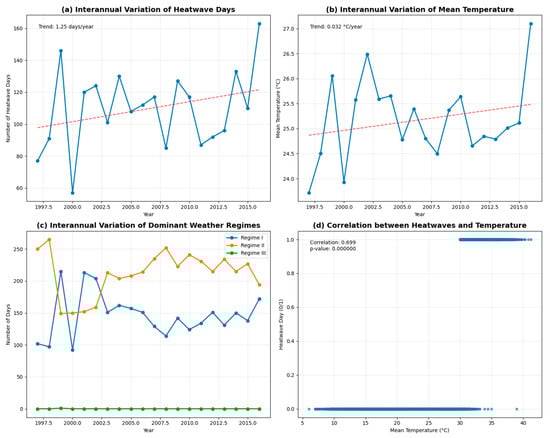
Figure 15.
Climate change impacts (1997–2016) on heatwave days and weather regimes. (a) Annual heatwave days with linear trend (~1.25 days yr−1). (b) Annual mean daily temperature trend (~0.032 °C yr−1). (c) Interannual evolution of weather regimes: Regime I declines, Regime II rises, Regime III remains rare. (d) Scatter plot of daily heatwave occurrence versus mean temperature, showing strong positive correlation (r = 0.699, p < 0.001).
Together, these panels reveal the synchronous rise in heatwaves and background temperature in recent years and reflect the evolving trends and shifting relative importance of different weather regimes under climate warming.
4.3. Climate Warming Background and Risk Implications
Based on projections from the Coupled Model Intercomparison Project Phase 6 (CMIP6) under the Shared Socioeconomic Pathway 5–8.5 (SSP5–8.5)—a high-emissions scenario consistent with continued fossil fuel use and limited climate mitigation—heatwaves in India are projected to intensify and exhibit increasing spatial–temporal heterogeneity. By 2041–2060, the national mean annual number of heatwave days is expected to increase by 7–8 days (≈0.3 d a−1) relative to 1995–2014, rising further to 10–17 days by 2076–2100. Regional contrasts are pronounced: the western Himalayas and northwest India may experience increases of up to 24 and 19 days, respectively. For extreme-threshold events, the area exposed to daily maximum temperatures above 43 °C is projected to expand by approximately 16-fold along the west coast and 10-fold along the east coast, with smaller (1–3-fold) expansions across other regions. Long-duration heatwaves (≥7 days) may increase more than 20-fold on the west coast, 12-fold over the inland peninsula, and eight-fold in the north-central, east coast, and western Himalayan zones. Coastal areas are expected to mainly experience intensity increases (>1.5 °C), whereas the northwest and western Himalaya are projected to undergo large frequency surges—together indicating a future compound risk pattern in which “high-frequency” events coexist with “high-intensity, long-duration” extremes [].
Regional Earth system modeling can further refine heatwave categories. By the 2080s, both dry–hot and humid–hot heatwave frequencies in India are expected to roughly double, single-event durations to increase by 8–12 days, and peak intensities to rise by 2–3 °C []. Under global warming of +2 °C, the annual frequency of compound (high-temperature + high-humidity) extremes is expected to increase by ≈ 5 times, with the upper quartile of event durations expanding to 5–25 days []. CMIP6 multi-model means also indicate an overall decrease in Northern Hemisphere summer blocking frequency—particularly over the Atlantic–Eurasian sector—under future warming [], echoing the slight decline of Regime I in Figure 15c. Notably, while prior studies typically classify Indian heatwaves into broad “dry–hot” or “humid–hot” types, our regime-based clustering captures finer dynamical nuances—such as the westward-shifted South Asian High and persistent blocking patterns—that are often missed by traditional categorizations. This enhances the resolution and applicability of early-warning protocols. Meanwhile, preprint analyses show that Bay of Bengal vorticity coupled with midlatitude anticyclones strengthens significantly under warming, compounded by a westward-strengthened South Asian High, favoring the long tail amplification of Regime III []. The 850 hPa pre-monsoon westerly jet has shifted northward by about 3° latitude and weakened by ≈25% since the 1980s—one study attributes this primarily to anthropogenic forcing []—further exacerbating extreme dry-invasion events.
The early-season heatwave from April to June 2024 drove Delhi’s average May maximum temperature up to 41.4 °C [], and World Weather Attribution estimates that warming has made such early-season events about 30 times more likely []. During the same heatwave, air conditioning and cooling demand accounted for 31–34% of the national peak load, directly increasing coal-fired generation []. Under the SSP5-8.5 scenario, the average duration and frequency of heatwaves in 100 “smart cities” nearly doubled, with some inland and coastal cities seeing duration increases approaching 100% []. Reviews also indicate that annual exposure days for the elderly and young children have risen significantly, accompanied by steadily increasing heat-related mortality in many locations []. Public health research further argues that highly exposed cities must integrate regime-based early warnings with time-of-use electricity pricing, cooling centers, and community support networks to protect low-income and outdoor labor populations [].
Studies show that scenario-based, locally tailored adaptation measures can significantly reduce economic losses from extreme climate events. For example, a normalization study in Odisha demonstrated that, after incorporating local adaptation practices, climate disaster losses declined markedly []. Our observational evidence, together with multi-model projections, consistently reveals that heatwave spectra are evolving toward a “Regime I: fewer but stronger” pattern and a “Regime III: elevated long-tail” risk. To reduce the growing multi-sector risks before the South Asian monsoon arrives (around May), several key measures should be put into practice: (1) start monitoring earlier, in late April or early May, with special attention to 500 hPa blocking patterns, soil moisture deficits, and jet stream shifts; (2) integrate automated regime identification into forecasting systems to provide longer lead times; (3) implement demand-side management strategies—like time-of-use pricing and reserve dispatch—to handle over 30% of peak electricity loads; and (4) roll out “Heat-Health Action Plans” in the most vulnerable cities, including cooling centers and community support networks. These integrated strategies are crucial for safeguarding energy security and public health—and for alleviating the earlier onset and longer persistence of extreme heatwaves under ongoing warming. These integrated strategies, grounded in our regime-based framework, are essential for ensuring energy security, protecting public health, and adapting to the earlier and more persistent heat extremes under continued global warming.
5. Conclusions
In this study, we used hourly observations from Delhi spanning from 1997 to 2016, applying K-means clustering (K = 3), an absolute-threshold heatwave criterion, and multiple statistical tests to develop a weather-regime framework for heatwave risk: dry-heat high-pressure (Regime I), mild–humid (Regime II), and blocking dry invasion (Regime III). Regime I, which occurred on 41% of days, accounts for 63% of heatwave days, representing a “high-frequency, moderate-to-long-duration” pattern. In contrast, Regime III appeared on less than 1% of days but produces the strongest and longest heatwaves under conditions of blocking and dry air intrusion—a “few-but-fierce” long-tail threat. Notably, the first heatwave of the season is arriving earlier, advancing by 0.57 days per year, while the total number of heatwave days is increasing by 1.25 days per year. Both trends are closely linked to a warming rate of 0.032 °C per year, highlighting a lengthening and intensifying heatwave season.
These findings are consistent with recent India-wide analyses reporting more frequent and severe heatwaves [,]. By classifying synoptic weather regimes and linking them to multi-day mean-temperature thresholds, the workflow embeds circulation drivers such as blocking and dry-air intrusions into the heatwave definition, improving interpretability and robustness [,]. Using Tmean thresholds also better captures limited nighttime cooling and cumulative heat stress, consistent with emerging health evidence []. Compared with single-indicator or subjective clustering approaches, this regime-based method is more robust, physically interpretable, and directly aligned with IMD operational thresholds for early warning [,].
This typology enhances our understanding of the spatiotemporal patterns of heatwaves and provides a robust physical–statistical foundation for targeted warnings, demand-side power management, and public health protection. However, this study has limitations: it relies on single-station data over 20 years (Regime III, n = 1) and includes only four conventional meteorological variables, without accounting for soil moisture, radiation, or human stress indices. These constraints point to the need for further research: integrating multi-station and reanalysis datasets, employing high-resolution land–atmosphere models, adopting relative-threshold or heat index criteria for compound extremes, and exploring spectral clustering or hidden Markov models to better capture regime transitions, improve mechanistic understanding, and extend early warning lead times.
Although this study was developed and tested for Delhi, the proposed regime-based heatwave risk classification and early-warning workflow are broadly applicable to other countries and cities with different climatic conditions. With minor adjustments to local meteorological data and heatwave threshold definitions, this framework can support targeted heat-risk assessments, guide demand-side energy management, and strengthen public health preparedness in rapidly urbanizing and climate-vulnerable regions worldwide. To facilitate such transfer, we summarize the methodological workflow as four key steps: (1) collect and preprocess local meteorological data at hourly or daily resolution, extending to additional variables such as soil moisture, radiation, or thermal stress indices where available; (2) standardize and, if necessary, reduce the dimensionality of the selected features (for example, through principal component analysis); (3) perform objective weather-regime classification using optimized clustering validated by internal indices and robustness tests; and (4) link the identified regimes to region-specific extreme-heat thresholds to quantify risk and inform operational early-warning systems. Clearly describing these steps allows researchers and practitioners to adapt the approach to other climates, data infrastructures, or related extreme-weather risk studies after integrating locally relevant datasets.
Author Contributions
Conceptualization, Y.L. and C.Z.; methodology, Y.L.; software, Z.D.; validation, Y.L., C.Z., and Z.J.; formal analysis, Y.L.; investigation, Y.L.; resources, C.Z.; data curation, Z.D.; writing—original draft, Y.L.; writing—review and editing, C.Z. and Z.J.; visualization, Z.D.; supervision, C.Z.; project administration, C.Z.; funding acquisition, Z.D. All authors have read and agreed to the published version of the manuscript.
Funding
This research received no external funding.
Institutional Review Board Statement
Not applicable.
Informed Consent Statement
Not applicable.
Data Availability Statement
The original contributions presented in this study are included in this article. Further inquiries can be directed to the corresponding author.
Acknowledgments
Declaration of generative AI and AI-assisted technologies in the writing process: during the preparation of this work, the authors used ChatGPT 4 in order to improve their language. After using this tool, the authors reviewed and edited the content as needed and take full responsibility for the content of the publication.
Conflicts of Interest
The authors declare no conflicts of interest.
Appendix A

Figure A1.
Sensitivity analysis: heatwave rate by cluster (k = 2, 3, 4).

Figure A2.
Clustering validity indices vs. number of clusters.

Figure A3.
Bootstrap stability: ARI distribution (KMeans, k = 3, B = 100).

Figure A4.
Weather regime transition matrices.
Table A1.
Sensitivity analysis of cluster number (k = 2, 3, 4) on heatwave risk typing.
Table A1.
Sensitivity analysis of cluster number (k = 2, 3, 4) on heatwave risk typing.
| k | Cluster | n_Days | Heatwave_Days | Heatwave_Rate (%) | Tmean_Avg | Hmean_Avg |
|---|---|---|---|---|---|---|
| 2 | 0 | 4232 | 347 | 8.2 | 21.3 | 68.64 |
| 2 | 1 | 2929 | 1846 | 63.02 | 30.84 | 43.6 |
| 3 | 0 | 2929 | 1845 | 62.99 | 30.84 | 43.61 |
| 3 | 1 | 4231 | 347 | 8.2 | 21.29 | 68.64 |
| 3 | 2 | 1 | 1 | 100 | 35.46 | 18.31 |
| 4 | 0 | 2151 | 1376 | 63.97 | 31.08 | 38.17 |
| 4 | 1 | 2487 | 0 | 0 | 16.46 | 66.93 |
| 4 | 2 | 2522 | 816 | 32.36 | 28.8 | 67.25 |
| 4 | 3 | 1 | 1 | 100 | 35.46 | 18.31 |
Table A2.
Comparison of heatwave risk typing by different clustering algorithms (k = 3).
Table A2.
Comparison of heatwave risk typing by different clustering algorithms (k = 3).
| Algorithm | Cluster | n_Days | Heatwave_Days | Heatwave_Rate (%) | Tmean_Avg | Hmean_Avg |
|---|---|---|---|---|---|---|
| KMeans | 0 | 2929 | 1845 | 62.99 | 30.84 | 43.61 |
| KMeans | 1 | 4231 | 347 | 8.2 | 21.29 | 68.64 |
| KMeans | 2 | 1 | 1 | 100 | 35.46 | 18.31 |
| GMM | 0 | 68 | 11 | 16.18 | 22.45 | 65.11 |
| GMM | 1 | 7092 | 2181 | 30.75 | 25.23 | 58.34 |
| GMM | 2 | 1 | 1 | 100 | 35.46 | 18.31 |
| Agglomerative | 0 | 3890 | 2188 | 56.25 | 30.84 | 54.08 |
| Agglomerative | 1 | 1 | 1 | 100 | 35.46 | 18.31 |
| Agglomerative | 2 | 3270 | 4 | 0.12 | 18.48 | 63.54 |
References
- Perkins, S.E.; Alexander, L.V. On the measurement of heatwaves. J. Clim. 2013, 26, 4500–4517. [Google Scholar] [CrossRef]
- Perkins, S.E. A review on the scientific understanding of heatwaves—Their measurement, driving mechanisms, and changes at the global scale. Atmos. Res. 2015, 164, 242–267. [Google Scholar] [CrossRef]
- McMichael, A.J.; Lindgren, E. Climate change: Present and future risks to health, and necessary responses. J. Intern. Med. 2011, 270, 401–413. [Google Scholar] [CrossRef] [PubMed]
- Westerling, A.L.; Hidalgo, H.G.; Cayan, D.R.; Swetnam, T.W. Warming and earlier spring increase western US forest wildfire activity. Science 2006, 313, 940–943. [Google Scholar] [CrossRef]
- McEvoy, D.; Ahmed, I.; Mullett, J. The impact of the 2009 heatwave on Melbourne’s critical infrastructure. Local Environ. 2012, 17, 783–796. [Google Scholar] [CrossRef]
- Rübbelke, D.; Vögele, S. Impacts of climate change on European critical infrastructures: The case of the power sector. Environ. Sci. Pol. 2011, 14, 53–63. [Google Scholar] [CrossRef]
- Zuo, J.; Pullen, S.; Palmer, J.; Bennetts, H.; Chileshe, N.; Ma, T. Impacts of heatwaves and corresponding measures: A review. J. Clean. Prod. 2015, 92, 1–12. [Google Scholar] [CrossRef]
- Keellings, D.; Waylen, P. Increased risk of heatwaves in Florida: Characterizing changes in bivariate heatwave risk using extreme value analysis. Appl. Geogr. 2014, 46, 90–97. [Google Scholar] [CrossRef]
- Pachauri, R.K.; Meyer, L.A.; Allen, M.R.; Barros, V.R.; Broome, J.; Cramer, W.; Christ, R.; Church, J.A.; Clarke, L.; Dahe, Q. Climate Change 2014: Synthesis Report. Contribution of Working Groups I, II and III to the Fifth Assessment Report of the Intergovernmental Panel on Climate Change; Core Writing Team, Pachauri, R.K., Meyer, L.A., Eds.; IPCC: Geneva, Switzerland, 2014; 151p. [Google Scholar] [CrossRef]
- Perkins-Kirkpatrick, S.E.; Lewis, S.C. Increasing trends in regional heatwaves. Nat. Commun. 2020, 11, 3357. [Google Scholar] [CrossRef]
- Dodman, D.; Hayward, B.; Pelling, M.; Castan Broto, V.; Chow, W.; Chu, E.; Dawson, R.; Khirfan, L.; McPhearson, T.; Prakash, A. Cities, Settlements and Key Infrastructure. In Climate Change 2022: Impacts, Adaptation and Vulnerability. Contribution of Working Group II to the Sixth Assessment Report of the Intergovernmental Panel on Climate Change; Pörtner, H.-O., Roberts, D.C., Tignor, M., Poloczanska, E.S., Mintenbeck, K., Alegría, A., Craig, M., Langsdorf, S., Löschke, S., Möller, V., et al., Eds.; Cambridge University Press: Cambridge, UK; New York, NY, USA, 2022; pp. 907–1040. [Google Scholar] [CrossRef]
- Liao, S.; Pan, W.; Wen, L.; Chen, R.; Pan, D.; Wang, R.; Hu, C.; Duan, H.; Weng, H.; Tian, C.; et al. Temperature-related hospitalization burden under climate change. Nature 2025, 644, 960–968. [Google Scholar] [CrossRef]
- Yenneti, K.; Tripathi, S.; Wei, Y.D.; Chen, W.; Joshi, G. The truly disadvantaged? Assessing social vulnerability to climate change in urban India. Habitat Int. 2016, 56, 124–135. [Google Scholar] [CrossRef]
- Gupta, A.K.; Negi, M.; Nandy, S.; Kumar, M.; Singh, V.; Valente, D.; Petrosillo, I.; Pandey, R. Mapping socio-environmental vulnerability to climate change in different altitude zones in the Indian Himalayas. Ecol. Indic. 2020, 109, 105787. [Google Scholar] [CrossRef]
- Hughes, S. Justice in urban climate change adaptation: Criteria and application to Delhi. Ecol. Soc. 2013, 18, 48. [Google Scholar] [CrossRef]
- Picciariello, A.; Colenbrander, S.; Bazaz, A.; Roy, R. The Costs of Climate Change in India: A Review of the Climate-Related Risks Facing India, and Their Economic and Social Costs; Overseas Development Institute: London, UK, 2021; Available online: https://odi.cdn.ngo/media/documents/ODI-JR-CostClimateChangeIndia-final.pdf (accessed on 10 July 2025).
- Mora, C.; Dousset, B.; Caldwell, I.R.; Powell, F.E.; Geronimo, R.C.; Bielecki, C.R.; Counsell, C.W.W.; Dietrich, B.S.; Johnston, E.T.; Louis, L.V.; et al. Global risk of deadly heat. Nat. Clim. Change 2017, 7, 501–506. [Google Scholar] [CrossRef]
- Raymond, C.; Matthews, T.; Horton, R.M. The emergence of heat and humidity too severe for human tolerance. Sci. Adv. 2020, 6, eaaw1838. [Google Scholar] [CrossRef]
- Kiarsi, M.; Amiresmaili, M.; Mahmoodi, M.R.; Farahmandnia, H.; Nakhaee, N.; Zareiyan, A.; Aghababaeian, H. Heatwaves and adaptation: A global systematic review. J. Therm. Biol. 2023, 116, 103588. [Google Scholar] [CrossRef]
- Poljansek, K.; Marín Ferrer, M.; De Groeve, T.; Clark, I. Science for Disaster Risk Management 2017: Knowing Better and Losing Less; Publications Office of the European Union: Luxembourg, 2017. [Google Scholar] [CrossRef]
- India Meteorological Department. Current Temperature Status and Heatwave Warning. IMD Bulletin. Available online: https://mausam.imd.gov.in/responsive/heatwave_guidance.php (accessed on 30 June 2025).
- Liu, J.; Kim, H.; Hashizume, M.; Lee, W.; Honda, Y.; Kim, S.E.; He, C.; Kan, H.; Chen, R. Nonlinear exposure-response associations of daytime, nighttime, and day-night compound heatwaves with mortality amid climate change. Nat. Commun. 2025, 16, 635. [Google Scholar] [CrossRef]
- He, C.; Kim, H.; Hashizume, M.; Lee, W.; Honda, Y.; Kim, S.E.; Kinney, P.L.; Schneider, A.; Zhang, Y.; Zhu, Y.; et al. The effects of night-time warming on mortality burden under future climate change scenarios: A modelling study. Lancet Planet. Health 2022, 6, e648–e657. [Google Scholar] [CrossRef]
- Carr, D.; Falchetta, G.; Sue Wing, I. Population aging and heat exposure in the 21st century: Which US regions are at greatest risk and why? Gerontologist 2024, 64, gnad050. [Google Scholar] [CrossRef]
- Reddy, E.A.; Rajan, K.S. Spatiotemporal Cluster Analysis of Gridded Temperature Data—A Comparison Between K-means and MiSTIC. arXiv 2023, arXiv:2307.00480. [Google Scholar]
- Shahfahad; Talukdar, S.; Islam, A.R.M.T.; Das, T.; Naikoo, M.W.; Mallick, J.; Rahman, A. Application of advanced trend analysis techniques with clustering approach for analysing rainfall trend and identification of homogenous rainfall regions in Delhi metropolitan city. Environ. Sci. Pollut. Res. 2023, 30, 106898–106916. [Google Scholar] [CrossRef]
- Rohini, P.; Rajeevan, M. An Analysis of Prediction Skill of Heat Waves Over India Using TIGGE Ensemble Forecasts. Earth Space Sci. 2023, 10, e2020EA001545. [Google Scholar] [CrossRef]
- Jain, A.K. Data clustering: 50 years beyond K-means. Pattern Recogn. Lett. 2010, 31, 651–666. [Google Scholar] [CrossRef]
- Arbelaitz, O.; Gurrutxaga, I.; Muguerza, J.; Pérez, J.M.; Perona, I. An extensive comparative study of cluster validity indices. Pattern Recogn. 2013, 46, 243–256. [Google Scholar] [CrossRef]
- Hennig, C. What are the true clusters? Pattern Recogn. Lett. 2015, 64, 53–62. [Google Scholar] [CrossRef]
- Mitchell, B.C.; Chakraborty, J.; Basu, P. Social Inequities in Urban Heat and Greenspace: Analyzing Climate Justice in Delhi, India. Int. J. Environ. Res. Public Health 2021, 18, 4800. [Google Scholar] [CrossRef]
- Pfahl, S.; Wernli, H. Quantifying the relevance of atmospheric blocking for co-located temperature extremes in the Northern Hemisphere on (sub-)daily time scales. Geophys. Res. Lett. 2012, 39, 12. [Google Scholar] [CrossRef]
- Miralles, D.G.; Teuling, A.J.; Van Heerwaarden, C.C.; Vilà-Guerau de Arellano, J. Mega-heatwave temperatures due to combined soil desiccation and atmospheric heat accumulation. Nat. Geosci. 2014, 7, 345–349. [Google Scholar] [CrossRef]
- Dodla, V.B.; Satyanarayana, G.C.; Desamsetti, S. Analysis and prediction of a catastrophic Indian coastal heatwave of 2015. Nat. Hazards 2017, 87, 395–414. [Google Scholar] [CrossRef]
- Jha, R.; Mondal, A.; Ghosh, S.; Murtugudde, R. Northward shift of pre-monsoon zonal winds exacerbating heatwaves over India. Geophys. Res. Lett. 2024, 51, e2024GL110486. [Google Scholar] [CrossRef]
- India Meteorological Department. FAQ on Heat Wave; Ministry of Earth Sciences, IMD: New Delhi, India, 2025. [Google Scholar]
- Liu, J.; Li, X. Characteristics and Driving Mechanisms of Heatwaves in China During July and August. Atmosphere 2025, 16, 434. [Google Scholar] [CrossRef]
- Satyanarayana, G.C.; Rao, D.V.B. Phenology of heatwaves over India. Atmos. Res. 2020, 245, 105078. [Google Scholar] [CrossRef]
- Pai, D.S.; Nair, S.A.; Ramanathan, A.N. Long-term climatology and trends of heatwaves over India during the recent 50 years (1961–2010). Mausam 2013, 64, 585–604. [Google Scholar] [CrossRef]
- Davini, P.; D’Andrea, F. From CMIP3 to CMIP6: Northern Hemisphere atmospheric blocking simulation in present and future climate. J. Clim. 2020, 33, 10021–10038. [Google Scholar] [CrossRef]
- Chattopadhyay, R.; Pai, D.S. Dynamics of Heatwave Intensification over the Indian Region. arXiv 2024, arXiv:2407.04256. [Google Scholar] [CrossRef]
- Upadhyaya, P.; Mishra, S.K.; Fasullo, J.T.; Kang, I.S. Attributing the recent weakening of the South Asian subtropical westerlies. npj Clim. Atmos. Sci. 2024, 7, 283. [Google Scholar] [CrossRef]
- Express News Service. 5 Heatwave Days, Little Rain: Capital Sees Its Hottest May Since 2013. The Indian Express. Available online: https://indianexpress.com/article/cities/delhi/5-heatwave-days-little-rain-capital-sees-its-hottest-may-since-2013-9364653/ (accessed on 17 July 2025).
- World Weather Attribution. Climate Change Made Devastating Early Heat in India and Pakistan 30 Times More Likely. Available online: https://www.worldweatherattribution.org/climate-change-made-devastating-early-heat-in-india-and-pakistan-30-times-more-likely (accessed on 18 July 2025).
- Ember. Powering Through the Heat: How 2024 Heatwaves Reshaped Electricity Demand (Insight Report). Available online: https://ember-climate.org/insights/research/powering-through-the-heat-how-2024-heatwaves-reshaped-electricity-demand/ (accessed on 18 July 2025).
- Goyal, M.K.; Singh, S.; Jain, V. Heatwave characteristics intensification across Indian smart cities. Sci. Rep. 2023, 13, 14786. [Google Scholar] [CrossRef]
- Mourougan, M.; Tiwari, A.; Limaye, V.; Matzarakis, A.; Singh, A.K.; Ghosh, U.; Pal, D.; Lahariya, C. Heat Stress in India: A Review. Prev. Med. Res. Rev. 2024, 1, 140–147. [Google Scholar] [CrossRef]
- Dasgupta, P.; Dayal, V.; Dasgupta, R.; Ebi, K.L.; Heaviside, C.; Joe, W.; Kolli, R.K.; Mehra, M.K.; Mishra, A.; Raghav, P. Responding to heat-related health risks: The urgency of an equipoise between emergency and equity. Lancet Planet. Health 2024, 8, e933–e936. [Google Scholar] [CrossRef]
- Bahinipati, C.S.; Venkatachalam, L. Role of climate risks and socio-economic factors in influencing the impact of climatic extremes: A normalisation study in the context of Odisha, India. Reg. Environ. Chang. 2016, 16, 177–188. [Google Scholar] [CrossRef]
- de Bont, J.; Nori-Sarma, A.; Stafoggia, M.; Banerjee, T.; Ingole, V.; Jaganathan, S.; Mandal, S.; Rajiva, A.; Krishna, B.; Kloog, I.; et al. Impact of heatwaves on all-cause mortality in India: A comprehensive multi-city study. Environ. Int. 2024, 184, 108461. [Google Scholar] [CrossRef]
- Council on Energy, Environment and Water (CEEW). How Extreme Heat is Impacting India: Mapping Climate Risks and Impacts of Extreme Heatwave Disaster in Indian Districts. Report. 2025. Available online: https://www.ceew.in/sites/default/files/mapping-climate-risks-and-impacts-of-extreme-heatwave-disaster-in-indian-districts.pdf (accessed on 1 October 2025).
- Barriopedro, D.; Fischer, E.M.; Luterbacher, J.; García-Herrera, R.; Ordóñez, C.; Miralles, D.G.; Salcedo-Sanz, S. Heat waves: Physical understanding and scientific challenges. Rev. Geophys. 2023, 61, e2022RG000780. [Google Scholar] [CrossRef]
- Royé, D.; Sera, F.; Tobías, A.; Hashizume, M.; Honda, Y.; Kim, H.; Vicedo-Cabrera, A.M.; Tong, S.; Lavigne, E.; MCC Collaborative Research Network; et al. Short-Term Association between Hot Nights and Mortality: A Multicountry Analysis in 178 Locations Considering Hourly Ambient Temperature. Environ. Int. 2025, 203, 109719. [Google Scholar] [CrossRef]
- Banerjee, A.; Gupta, S.; Priyanshu, P.; Kar, A.; Saha, R.; Chakraborty, T.; Ghosh, D.; Kurths, J.; Hens, C. Recent changes in spatiotemporal patterns of heat extremes in South Asia. npj Clim. Atmos. Sci. 2025, 8, 293. [Google Scholar] [CrossRef]
Disclaimer/Publisher’s Note: The statements, opinions and data contained in all publications are solely those of the individual author(s) and contributor(s) and not of MDPI and/or the editor(s). MDPI and/or the editor(s) disclaim responsibility for any injury to people or property resulting from any ideas, methods, instructions or products referred to in the content. |
© 2025 by the authors. Licensee MDPI, Basel, Switzerland. This article is an open access article distributed under the terms and conditions of the Creative Commons Attribution (CC BY) license (https://creativecommons.org/licenses/by/4.0/).