Abstract
Physiological equivalent temperature (PET) is one of most used indices for outdoor human well-being evaluation; its determination is particularly helpful for adaptation strategies in built-up areas affected by the urban heat island (UHI) phenomenon. In this work, we presented a methodology to compute spatially and temporally resolved PET values during a heatwave at the city level, based on a combination of satellite products, in situ measurements and Envi-met model runs upscaled from specific test areas to the broader city. The method exploits the ECOSTRESS sensor to detect surface thermal patterns at different diurnal times by developing an hourly based index called hUHTI (hourly urban heatwave thermal index) that serves as a proxy. A case study on Prato (Italy) municipality during the 2021 summer heatwave events is presented. Based on the available satellite products, a set of six hourly diurnal PET maps at 10 m spatial resolution were derived and daytime outdoor thermal patterns and trends were investigated according to land cover. hUHTI index resulted a more suitable tool as PET proxy compared to the sole ECOSTRESS land surface temperature (LST) product, especially for morning and evening times. Hourly PET maps were summarized by the use of an average exceedance map providing public administrations and stakeholders a synthetic tool for urban regeneration purposes at city scale.
1. Introduction
Urban heat islands (UHI) [1] are the result of highly concentrated structures such as buildings, industries, roads, and other infrastructures absorbing and releasing heat from the sun, and limited greenery, which make urban areas warmer compared to surrounding areas. Heat islands can form in a variety of conditions, including day or night, large or small cities, suburbs, northern or southern climates, and any time of year [2]. The temperature difference between cities and their surroundings is typically used to quantify heat islands. Within a city, the temperature can also change due to the non-uniform distribution of heat-absorbing pavements and buildings; some areas become hotter than others while others remain cooler thanks to trees and other vegetation. In this context, the increasing global warming trends are quickly and severely impacting the current outdoor thermal environment of urban areas, increasing building cooling loads, reducing indoor comfort, and enhancing the risks of heat-related mortality [3,4]. This trend is expected to increase, leading to a reduction in the city’s livability and vitality on a physical, economic, environmental, and social level [5].
The determination of urban heat maps is usually performed using different approaches: (i) land surface temperatures (LST) retrieved by satellites and (ii) spatial interpolation of air temperatures (Tair) acquired by sensors mounted on fixed meteorological stations or traverses of vehicles. The first method is the most used, providing simultaneous land surface temperature measurements for the study of surface urban heat island (SUHI) [6] in a given area. However, it is important to note that SUHI may significantly differ from atmospheric UHI [7]: during the day, surface temperatures are more variable than atmospheric air temperatures, while at night, they are often similar. When compared to UHI, the fundamental characteristics of SUHI typically diverge during the day, when the sun is at high solar angles, and in the summer when SUHI is more intense; furthermore, it exhibits greater temporal and spatial variation than atmospheric UHI [8].
Several studies aimed at finding a relationship between surface and atmosphere temperatures [9,10,11] to understand how the materials of urban surfaces influence the temperature of the air above, but uncertainties are significant, especially in urban environments. The topic is still of scientific interest [12,13,14,15,16].
The diurnal patterns of SUHI and UHI phenomena are characterized by high spatial and temporal variability [17]. These patterns, especially for SUHI, were rarely investigated because traditional satellites and sensors flying on polar orbits (such as Landsat, MODIS, Sentinel constellation) have no diurnal sampling data, acquiring data always at the same time. The Ecosystem Spaceborne Thermal Radiometer Experiment on Space Station (ECOSTRESS) launched in 2018 allows us to investigate the thermal diurnal cycling of LST and SUHI, since it acquires not only at high spatial (70 m) and temporal (revisit time around 4 days in Europe) resolution, but also at varying times during day and night [18]. Despite the primary objective of ECOSTRESS being to answer critical science agricultural and environmental questions about water use and stress in plants, it was already used in several studies aimed at investigating and mitigating UHI [17,18,19,20,21]. In particular, Chang et al. and Hulley et al. [18,19] highlighted how in Los Angeles County (USA) and Xi’an metropolitan area (China), diurnal LST diurnal variations and patterns evolved according to various environmental and anthropic factors such as marine influence, materials with high heat capacity, orientation, asphalt depth shading, and weathering of urban landscape.
The determination of UHI maps so as further thermal comfort models can be highly useful to retrieve outdoor human well-being considering air temperature and other environmental parameters such as air humidity, wind speed, and surface radiant temperature [22,23,24]. Currently, one of the most used indices in outdoor environment is the physiological equivalent temperature (PET) [22,25,26]. This index, proposed by Höppe [27] and based on the Munich Energy-balance Model for Individuals (MEMI), is defined as the air temperature at which the human energy budget is maintained by skin temperature, core temperature, and sweat rate equal to those under the conditions being assessed [23]. Several studies proved the suitability of this model for hot-humid climates, probably because it uses standard clothing and activity, which are similar to what can be found in this type of climate. PET values can be expressed in degrees Celsius, making its interpretation more comprehensible to common people [22]. Moreover, based on the classification proposed in Matzarakis and Mayer [28] for Western/Middle Europe (Table S1), PET values can be associated with the grade of physiological stress and related thermal perception.
Since it is the combined result of physical and biophysical interactions between the earth surface (e.g., soil, buildings, vegetation), the atmosphere and the human body, the determination of PET is rather complex, especially when computed not punctually but for a whole area. Several models and software were developed for its calculation. Among them, Rayman [29] is one of the most used; it is a one-dimensional in space (all calculations are performed punctually) diagnostic model which calculates the radiation fluxes within the urban environment through morphological, meteorological, and thermo-physiological factors. SkyHelios [30,31] is a diagnostic model designed to estimate at small and micro scales (e.g., district, block, or street) spatially resolved atmospheric parameters, as well as thermal indices with low computational requirements. Envi-met [32] is a three-dimensional non-hydrostatic fluid dynamic microclimate model designed to simulate the surface–plant–air interactions within daily cycles in the urban environment with a typical resolution of 0.5 to 10 m in space and 10 s in time. This model, commonly employed for urban regeneration purposes through nature-based solutions (NBS) [33], was validated in several studies [34,35]. Due to computational and time constraints, Envi-met simulations are usually performed over areas not exceeding 1 km2 and with a maximum 5 m resolution. Envi-met is therefore not suitable to model in a single run the whole extension of medium–big–mega metropolitan areas. However, when Envi-met simulations are performed to support urban planning purposes, it is necessary to model the whole urban environment in order to provide stakeholders thematic maps that cover the entire urban area. Dividing the area in 1 km2 tiles, modelling each one and then merging the results in a final single map may not a be a viable solution because it is very time consuming and computationally challenging, especially when dealing with mega cities or big cities with extensive suburbs.
The objective of the present manuscript is to develop a methodology capable of computing spatially and temporally resolved PET values during a heatwave at the city level, based on a combination of satellite products, in situ measurements, and Envi-met model runs upscaled from specific test areas to the broader city. The method exploits the new opportunities offered by the ECOSTRESS sensor to detect surface thermal patterns at different diurnal times by developing an hourly based index called hUHTI (hourly urban heatwave index) that serves as a proxy. A case study relating to the municipal area of the city of Prato (central Italy) during the 2021 summer heatwave events is presented. The ability of hUHTI as a proxy for PET is compared with that of the ECOSTRESS LST products; finally, diurnal and exceedance PET trends and patterns are investigated according to the different land cover classes present in the study area.
2. Materials and Methods
2.1. Study Area
The study was conducted in the municipal area of Prato (43°52′48″ N, 11°05′54″ E), a town located in Toscana Region (Italy) with around 200,000 inhabitants. Part of the hilly, poorly inhabited northern part of the municipality was excluded since the 1 m spatial resolution DSM (Digital Surface Model) necessary for Sky View Factor (SVF) calculation was not available for this area. The study area (Figure 1) measured 80.98 km2 and its elevation ranged between 31 and 528 m a.s.l. with a gradient from south to north. A large part of the municipal territory extended over the flat area whose main land cover classes are different types of urban fabric (residential areas with discontinuous and sparse fabric, residential areas with continuous fabric, industrial and commercial areas) and agricultural areas; the hilly northern area was mostly covered by woodland and tree crops.
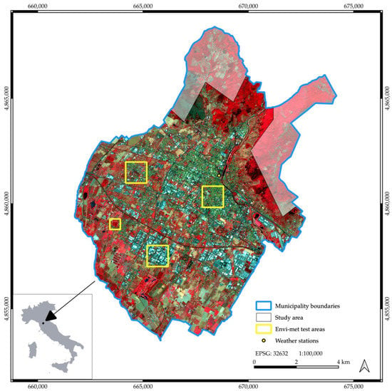
Figure 1.
Study area and location of Envi-met test areas. Background image: false color composite Sentinel 2 image acquired on 11 August 2021.
Prato has a mesothermal temperate climate with dry and hot summers and cool damp winters, classified as Csa in the Köppen and Geiger climate classification [36]. Mean annual temperature and mean total rainfall for the period 1991–2020 were 15.8 °C and 936 mm, with July and August recorded as the warmest months [37]. In recent years, the investigated area was often affected by heatwaves during the summer [38]. As there are various definitions of heatwaves, in this study, we embedded the definition of the Italian Ministry of Health [39], i.e., a period of three consecutive days with maximum temperature over 30 °C. The 2021 heatwave periods [37] for the study area are listed in Table 1. Heatwaves generated by high pressure systems in Central Italy are always characterized by calm wind and highly stable atmosphere [40].

Table 1.
2021 heatwaves in the study area.
2.2. Data Used in This Study
2.2.1. ECOSTRESS Dataset
The LST data used in this study were derived from ECOSTRESS Level-2 Land Surface Temperature and Emissivity product. The ECOSTRESS LST product uses a physics-based Temperature Emissivity Separation (TES) algorithm to dynamically retrieve LST from five ECOSTRESS thermal infrared bands with wavelength between 8 and 12.5 μm [18].
Scenes acquired during the daylight hours of 2021 heatwave days were selected. Cloud mask (CM) and quality check (QC) products were provided in the Level-2 imagery dataset to facilitate screening out aberrant data. For each scene, cloud and low-quality pixels were filtered out using the corresponding CM and QC files. Only filtered scenes covering the whole study area were selected for further steps; the 8 scenes composing the final ECOSTRESS LST dataset are listed in Table S2.
2.2.2. Sentinel 2 Dataset
Four Copernicus Sentinel-2 level- 2A high-resolution (10 m) raster products (Table S3) were extracted from the Copernicus Open Access Hub [41]. These scenes were chosen since they were not affected by clouds and within four days from the selected ECOSTRESS scenes (Table S2). The scenes were then used to calculate the normalized difference vegetation index (NDVI) [42] and to derive the related vegetation fraction cover (VFC) [43].
2.2.3. LIDAR Dataset
The 1 m spatial resolution digital surface model (DSM) raster layer provided by the Italian Ministry of the Environment obtained from airborne LIDAR (Light Detection and Ranging) data acquired in 2008 was used to derive the Sky View Factor (SVF) [44].
2.2.4. Meteorological and Land Cover Data
The meteorological data used in this study were retrieved from the weather station (reported in Figure 1) of the regional meteorological service of Toscana region (LaMMA Consortium).
The 2019 land cover classification available on the Toscana geoportal [45] was used to investigate diurnal PET trends and variations among land cover types. The original study area land cover legend (composed of 25 classes) was simplified to 15 classes according to the purposes of the investigation (Figure 2); related average SVF, VFC and LST values for each land cover class are given in Table 2.
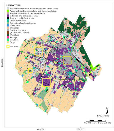
Figure 2.
Simplified land cover map of the study area derived from the 2019 land cover classification available on the Toscana geoportal [45].

Table 2.
Average sky view factor (SVF), vegetation fraction cover (VFC) and land surface temperature (LST) values for the classes of the simplified land cover map (Figure 2).
3. Methods
The flowchart for the proposed methodology is illustrated in Figure 3; it consists of five consecutive steps:
- Modelling Envi-met on test areas representative of the different urban fabrics in the monitored study area to derive hourly test areas PET maps;
- Developing a modified version of the UHTI index [14], named hUHTI, which exploits the daytime temporal acquisition variability provided by the ECOSTRESS sensor and is, therefore, capable of providing hourly study area outputs to be used as a PET proxy;
- Establishing simple linear regressive relationships between PET and hUHTI of the same time of the day;
- Spatializing the hourly PET test area maps using hUHTI of the same time as proxy though simple linear models to derive a set of hourly PET maps of the whole study area;
- Deriving a synthesis map, defined as exceedance map, which summarizes the information on thermal patterns of the hourly PET maps and can, thus, be exploited for urban planning purposes.
Apart from the first step, all the steps (including GIS data preparation, statistical analysis, map production) were performed using QGIS [46] and R (version 4.1.2) [47] software. The results of such methodology applied on the municipal area of Prato were analyzed according to the different land cover classes. In the following paragraphs, the method is explained in detail.
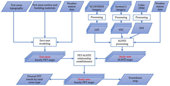

Figure 3.
Flowchart of implemented methodology (DSM = digital surface model; LST = land surface temperature; VFC = vegetation fraction cover; SVF = sky view factor; PET = physiological equivalent temperature; hUHTI = hourly urban heatwave thermal index).
3.1. Envi-Met Modelling
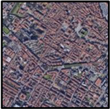
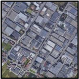
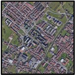
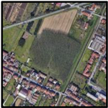
Envi-met modelling was performed over 4 test areas chosen to represent the main urban and land cover types present in the study area; their location and main characteristics are shown, respectively, in Figure 1 and Table 3.

Table 3.
Test areas used for Envi-met simulations and their characteristics [48].
All test area simulations were initialized with the same meteorological conditions recorded by the weather station (reported in Figure 1) of the LaMMA Consortium. The model simulated the microclimate conditions for the day (25 July) with the maximum temperature recorded during the 2019 summer heatwave. The chosen date was representative of the typical meteorological conditions in the study area during a heatwave, i.e., high temperatures, low wind speeds and a dry atmosphere (low relative humidity).
The input meteorological parameters were:
- Wind speed: 2.0 m/s;
- Wind direction: 70° from North;
- Maximum air temperature at h 14:00: 39.75 °C;
- Minimum air temperature at h 04:00: 24.07 °C;
- Maximum air relative humidity at h 4:00: 58%;
- Minimum air relative humidity at h 14:00: 15%.
The model ran for 36 h to have a full day simulation, since the first 12 h were excluded to avoid fluid dynamic instability and parameters initialization processes. Then, air temperature, radiant temperature, wind speed and specific humidity Envi-met modelling outputs were processed with the Bio-met tool to compute hourly PET maps for each test area with an output 5 m spatial resolution. Bio-met was set up using standard human body values (ISO 7730 [49]).
3.2. Hourly Urban Heatwave Thermal Index (hUHTI) Calculation
The procedure to calculate hUHTI was similar to that previously developed for UHTI index calculation [14]. Briefly, UHTI quantifies daytime air temperature variability patterns in an urban environment during a meteorological heatwave; the index takes into account three principal urban remotely sensed elements: (a) surface materials represented by LST, (b) vegetation represented by normalized difference vegetation index (NDVI) and (c) urban morphology expressed in terms of SVF; their relationship with ground data air temperatures is established through linear modelling, leading, after combination and normalization between 0 and 1, to thematic cartography to delineate city thermal patterns during a summer heatwave [14]. The higher the UHTI value, the more the area is thermally vulnerable during a heatwave. This modelling approach does not consider the wind component, since summer heatwave events in Central Italy are characterized by low wind speeds, high stable pressure field and clear sky. In addition, wind speed is slowed down in urban areas, especially due to the complex and dense urban geometry of the old historical centers typical of the Italian cities [40]. UHTI provides a general summer heatwave thermal characterization of the study area, since LST and NDVI input maps are the average of selected summer scenes relatives to a period of 4–5 years; moreover, UHTI depicts thermal patterns at midday since Landsat LST scenes used for its calculation are acquired at h 12.00 and Envi-met outputs used for SVF-Tair relationship establishment are selected at the same daytime. On the other hand, hUHTI was conceived to provide a thermal characterization of the study area at different diurnal daytimes, allowing to depict how thermal patterns evolve during the day; for such purpose, the hUHTI index exploits the temporal variability of ECOSTRESS acquisition (used for LST-Tair relationships) and the daytime variability of the SVF–Tair relationships, since they are calculated for the corresponding daytime. This leads to a set of hUHTI maps relative to different daytimes that are, therefore, ideal to spatialize the hourly Envi-met modelling PET outputs of the corresponding daytime.
In this study, 8 hUHTI maps were derived for the selected study area in 2021; the input remotely sensed files used for each one are listed in Table 4. Each hUHTI map was related to a day belonging to a 2021 heatwave (Table 2) and the selected days were characterized by similar meteorological characteristics (Table S4); this aspect implies that daytime hUHTI maps can be both used for the following steps of the method and investigated to detect trends of daytime thermal patterns.

Table 4.
List of the hUHTI maps calculated in the present investigation and the remotely sensed input layers used for their calculation.
Relationships between air temperature and input remote sensing LST and VFC layers were assessed using data of the weather station data located in Prato municipality (Figure 1) provided by LaMMA Consortium. Since the conceptual basis and the main processing steps are the same both for UHTI and hUHTI calculation, for an in-dept description of these aspects, we referred to [14]; here, we focus in the following paragraphs on the establishment of the relationships between LST, VFC, SVF and air temperatures for hUHTI calculation, since it slightly differs from the original procedure developed for UHTI calculation.
3.2.1. LST-Tair Relationship Establishment
To calculate LST-Tair relationship, the ECOSTRESS LST pixel values corresponding to the geolocation of the Prato weather station (Figure 1) were extracted for each scene of Table S2. Linear modelling was performed between extracted LST values and air temperature recorded by the weather station at the same date and time obtaining the following equation (R2 = 0.844, p value < 0.001) that was used for TLST calculation:
TLST = −0.55 (LST) + 11.99
3.2.2. SVF–Tair Relationship Establishment
Regarding SVF–Tair relationship establishment, in situ air temperatures could not be used because only one weather station was available in the study area (Figure 1), thus preventing, for this surface characteristic, the establishment of a relationship with measured air temperatures. For this reason, SVF-Tair relationships were established for each hUHTI map (Table 4) replacing air temperatures measured by the weather stations with Envi-met modelled air temperatures. The resulting regression parameters implemented for each SVF-Tair linear regression are provided in Table 5.

Table 5.
Regression parameters of the simple linear regressions between SVF and Tair.
3.2.3. VFC–Tair Relationship Establishment
The relationship between air temperature and VFC could not be established for the study area, since there were not enough weather stations with different values of VFC coverage available. Therefore, the relationship found for Bologna municipality [14] was used and is represented by the following equation (R2 = 0.893, p value < 0.05):
TVFC = −2.49(VFC) + 25.79
3.3. Hourly PET Map Spatialization and Comparison between ECOSTRESS LST and hUHTI as PET Predictors
The hUHTI previously described was used as regressor to upscale Envi-met PET outputs modelled for the test areas over the whole study area. Only the PET outputs corresponding to the daytime of the available hUHTI maps (Table 4) and relative to a height from the ground of 1.8 m were extracted and processed; these hourly PET test area grids were resampled to 10 m to fit with the hUHTI maps. Regarding hUHTI maps, a preliminary step involved building masking, since PET was conceived for outdoor comfort evaluation; therefore, simple linear relationships were built only using values corresponding to outdoor areas.
Each hUHTI map was reclassified into 10 classes using K-Means algorithm [50]; thus, for each selected daytime and each class, mean hUHTI and PET values were extracted and used for linear regression relationship establishment. Therefore, for each daytime, specific linear regressions were established and used to derive hourly PET maps for the whole study area with a spatial resolution of 10 m.
In order to assess whether hUHTI was a better PET predictor than LST alone, the same procedure described above was performed using ECOSTRESS LST instead of hUHTI, and regression metrics were compared.
3.4. Analysis of PET Diurnal Variations According to Land Cover and Crop Type
Average hourly PET values were extracted to investigate diurnal PET trends and variations among the various land cover types of the simplified 2019 land cover classification (Figure 2).
Moreover, since, during the analysis, it emerged that the crop phenological stage affected PET values in the cultivated areas, crop areas were classified to investigate and highlight this aspect. Two Sentinel 2 cloud free scenes were selected (acquired on 27 June and 21 August, respectively, DOY 178 and 233) and NDVI were computed. Annual crop areas (tree crops were excluded) of each scene were reclassified in two classes (H = values above 0.5, L = values below 0.5) leading to a cultivated areas classification (Figure 4) consisting of four classes: HH, HL, LH, LL.
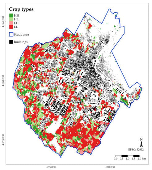
Figure 4.
Annual crop areas classification based on NDVI values relative to 22 June and 16 August 2021 (H = NDVI > 0.5; L = NDVI < 0.5).
3.5. Average PET Exceedance Map
In order to summarize hourly PET maps and provide a synthetic map of the areas most exposed to heat stress, an average exceedance heat map was derived. Koopmans et al. [51] used a conceptually similar map counting the number of hourly exceedances of a PET threshold where most persons feel outdoor thermal discomfort, i.e., 29 °C. In this study, we chose to compute the average of PET exceedance values over 35 °C PET (corresponding to strong heat stress according to the ranges of Table S1), believing that this solution highlights the severity of the heat stress in the most exposed areas.
4. Results
4.1. Envi-Met PET Simulations
A set of hourly PET test area maps was obtained through Envi-met simulations. PET daytime trends of the main test area land cover classes are shown in Figure 5. At early morning (h 06:00), differences between classes were moderate and all land cover classes fell in the slight heat stress grade of physiological stress, according to the classification proposed by Matzarakis et al. [28]. All land cover classes, except woodland, showed a sharp increase in PET values reaching the extreme heat stress grade already before 9 a.m. in the morning. PET values continued to grow until about 2 p.m. and a significant decrease was recorded only after 4 p.m.; for these classes, therefore, the extreme heat stress level lasted during a heatwave approximately 10 h per day, from h 8 a.m. to 6 p.m. The industrial and commercial areas (ICA) class showed the highest PET values. Regarding the two classes of urban fabric, residential areas with continuous fabric (RACF) and residential areas with discontinuous and sparse fabric (RADSF), it is interesting to note how the RACF class had lower PET values during the day than the RADSF due to the lower SVF values (Table 2); in the evening (h 20–21), however, this trend was reversed due to the thermal emission of the heat stored during the day by the buildings. The green urban areas (GUA) class showed slightly higher values than the RADSF and higher than the RACF in the early morning hours, but then, it was cooler in the central hours of the day. The woodland (W) class was the only one for which there was a less marked increase in PET in the morning; the extreme heat stress level was reached for about 6 h from 11 a.m. to 5 p.m.
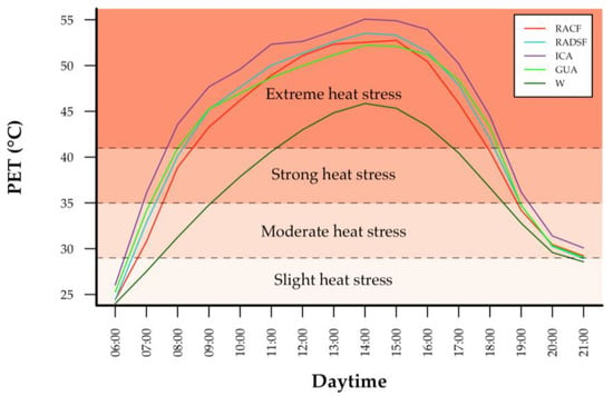
Figure 5.
Mean Envi-met modeled PET daytime trends for the main test area land cover classes. (RACF = residential areas with continuous fabric; RADSF = residential areas with discontinuous and sparse fabric; ICA = industrial and commercial areas; GUA = Green Urban Areas; W = woodland;). Background colors indicate the grade of physiological stress based on PET ranges for Western/Middle Europe (internal heat production: 80 W, heat transfer resistance of the clothing: 0.9 clo) according to Matzarakis et al. [28].
The PET maps obtained with Envi-met modelling for the four test areas at h 14:00 and at 1.8 m height are shown in Figure 6; a high grade of thermal stress (extreme heat stress according to Matzarakis et al. [28]) was evident, as can be expected during the central diurnal hours of a heatwave in Central Italy. The green area had the lowest PET values, but it is worth noting that bare soils of crops in the industrial test area showed PET values analogue to those of the paved and built surfaces. In the historical center, PET was generally lower compared to the two other urban areas due to lower SVF values (Table 2) that amplified buildings’ shadow effect. Extremely high values in the test areas were generally found in the proximity of buildings that are directly irradiated (southern exposure). Low PET values were generally found in residential and green areas with high tree vegetation coverage.
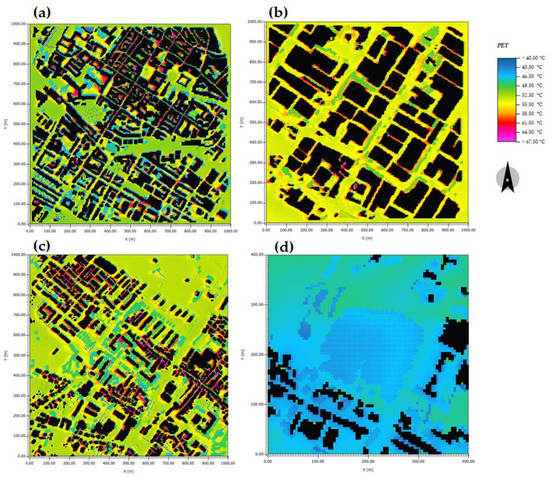
Figure 6.
1.8 m height PET at h 14:00 modelled with Envi-met software for the four test areas: (a) historical center; (b) industrial area; (c) residential area; (d) green area.
4.2. hUHTI Maps
A total of eight hUHTI maps, shown in Figure 7, were calculated for the following daytimes: 06:00, 07:00, 09:00, 11:00, 12:00, 13:00, 16:00, 21:00.
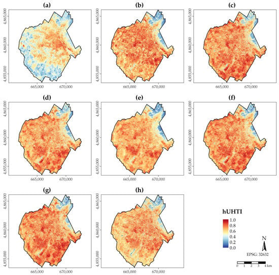
Figure 7.
Hourly Urban Heatwave Thermal Index (hUHTI) maps of the study area for different daytimes: (a) 06:00; (b) h 07:00; (c) h 09:00; (d) h 11:00; (e) h 12:00; (f) h 13:00; (g) h 16:00; (h) h 21:00.
In the early morning (h 06.00), the UHI phenomenon was clearly detectable; the urban fabric of Prato town and the surrounding commercial and industrial areas were much warmer than the surrounding areas, i.e., the woodland to the north and the agricultural areas to the south and west. During the day, the difference between the agricultural areas and the urban areas was less defined, unlike the woodland in the north which remained much cooler. Furthermore, during the day, the dense urban areas of the historical center were less “hot” than other areas such as commercial and industrial areas which in the warmest hours of the day were characterized by very high hUHTI values. The small cool spots (blue areas) were relative to green urban areas with high tree vegetation coverage. An interesting aspect that emerged is that cultivated areas did not show a unique and homogeneous behavior, but their thermal patterns varied among the different hUHTI maps. In the maps that implemented ECOSTRESS LST scenes acquired at the end of June (DOY 178, 174, 177 that provided LST information for hUHTI maps relative to, respectively, h 06.00, 07:00, 12.00 as listed in Table 4), urban areas were generally warmer than cropped areas and the typical UHI patterns were recognizable. For the hUHTI maps that implement ECOSTRESS LST acquired during the central part of August (DOY 230, 226, 233, 225 that provided LST information for hUHTI maps relative to, respectively, h 09:00, 11:00, 13:00, 16:00 as listed in Table 4), urban areas were much less recognizable and some fields (especially in the southern zone of the study area) had high hUHTI values, comparable to those of the warmest urban areas such the industrial and commercial areas.
4.3. PET Maps and Land Cover Trends
Figure 8 shows the coefficients of determination (R2) and relative statistical significance (p value) of simple linear regressions between hUHTI and PET Envi-met modeling outputs and between ECOSTRESS LST and PET Envi-met modeling outputs; the complete statistical parameters of the simple linear regressions are provided in Table S5. At h 06:00, linear models were characterized by low R2 values and were not statistically significant both for hUHTI and for ECOSTRESS LST; at h 07:00, linear relationship became strong and statistically significant for hUHTI, but not for ECOSTRESS LST. In the central hours of the day, linear relationships were always strong and statistically significant both for hUHTI and ECOSTRESS LST; in the evening (h 21:00), R2 values were lower, but still statistically significant. Overall, hUHTI showed higher coefficients of determination compared to those of ECOSTRESS LST, except for h 12:00 and 13:00 when the latter showed slightly stronger relationships with PET.
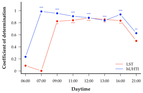
Figure 8.
Coefficients of determination (R2) related to simple linear regressions between ECOSTRESS Land Surface Temperatures (LST) and Envi-met modeled PET (red line) and related to simple linear regressions between hUHTI index and Envi-met modeled PET (blue line) at different daytimes (** = p value ≤ 0.01; *** = p value ≤ 0.001).
4.4. hUHTI—PET Hourly Relationships during Heatwave Event
Based on the PET-hUHTI relationship parameters shown in Table S5, PET maps were calculated and are shown in Figure 9. PET map relative to h 06:00 was not calculated because the simple linear relationship was not statistically significant (Figure 8 and Table S5). The PET map of h 21:00 was also excluded because, even if statistically significant, the simple linear relationship was less defined compared to the others since solar angle at sunset is very low and thermal patterns are also already influenced by nocturnal thermal dynamics. Due to the strong relationship between PET and hUHTI, attested by the very high R2 values, thermal patterns of PET maps were very similar to those of the hUHTI maps (Figure 7); however, the PET maps had the added value, compared to the corresponding hUHTI maps, of providing PET values which gave a more defined indication of the degree of thermal stress perceived at different times of the day.
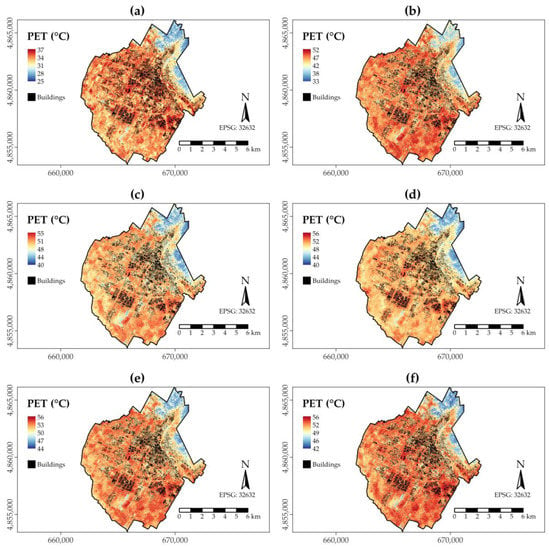
Figure 9.
Physiological Equivalent Temperature (PET) maps of the study area at different daytimes: (a) h 07:00; (b) h 09:00; (c) h 11:00; (d) h 12:00; (e) h 13:00; (f) h 16:00.
Mean PET values of each land cover class were calculated for each map and are available in Table S6; trends of the most important classes are shown in Figure 10. They all manifested an increase during the morning till h 13:00 and the beginning of the decrease at 16.00; however, differences between classes were quite marked and ranged around 5–6 °C between the warmest class (industrial and commercial areas, ICA) and the coolest (woodland, W). Urban residential areas did not show marked differences between continuous (RACF) and discontinuous and sparse (RADSF) fabric and, apparently surprisingly, revealed lower values compared to the urban green areas; however, it must be highlighted that in the study area, urban green areas were generally characterized by large meadows and a relatively low presence of trees.
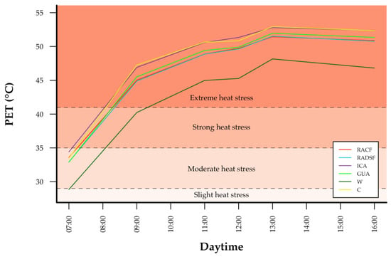
Figure 10.
Mean PET values at different daytimes for the main land cover classes (RACF = residential areas with continuous fabric; RADSF = residential areas with discontinuous and sparse fabric; ICA = industrial and commercial areas; GUA = Green Urban Areas; W = woodland; C = crops). Background colors indicate the grade of physiological stress based on PET ranges for Western/Middle Europe (internal heat production: 80 W, heat transfer resistance of the clothing: 0.9 clo) according to Matzarakis et al. [28].
Regarding crops, they showed high PET values, almost equal to those of the industrial and commercial areas; however, this PET trend was influenced by the acquisition day of the ECOSTRESS and Sentinel 2 scenes (Table 4) implemented to derive the hUHTI used for PET spatialization and the consequent crops’ phenological stage. In order to highlight this aspect, mean PET values were computed according to the four crop types shown in Figure 4 and their trends are shown in Figure 11. Differences were evident between HH and LL crop types; HH crops showed, as expected, always lower PET values compared to LL crops since the culture was active (high NDVI values) and temperatures were reduced by evapotranspiration. The situation was more complex for HL and LH crops, as their PET trends were influenced by the period in which the remotely sensed products used for that specific hourly PET map were acquired. HL crops showed higher PET values for those daytimes (h 09:00, 11:00, 13:00, 16:00) that implemented remotely sensed products acquired in mid-August; on the contrary, LH crops showed higher values for those daytimes which were obtained from remotely sensed products acquired at the end of June (h 07:00, 12:00).
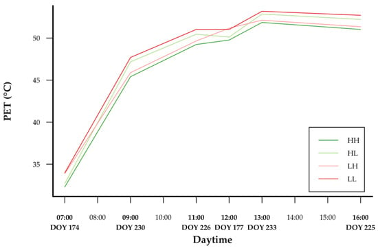
Figure 11.
Mean PET values at different daytimes for the four types of crops. DOY indicates at which day in 2021 the ECOSTRESS scene was acquired for the calculation of hUHTI used for PET spatialization over the whole study area.
4.5. Exceedance Map and Statistics
The average PET exceedance map (Figure 12) showed values between 4.5 and 16.6 °C, indicating that all different areas within the study area, including also rural woodland, were affected by diurnal strong thermal stress for at least some hours during a heatwave. Densely wooded urban green areas and woodland were the coldest (blue spots), whilst the warmest zones were the industrial and commercial areas, and most crop fields (red spots). Therefore, areas with the greatest thermal discomfort were those characterized by large expanses of asphalt or bare soil, where SVF and NDVI values were, respectively, very high and low; in such areas, there were no elements providing shade, such as buildings and trees, and (evapo)transpiration was low.
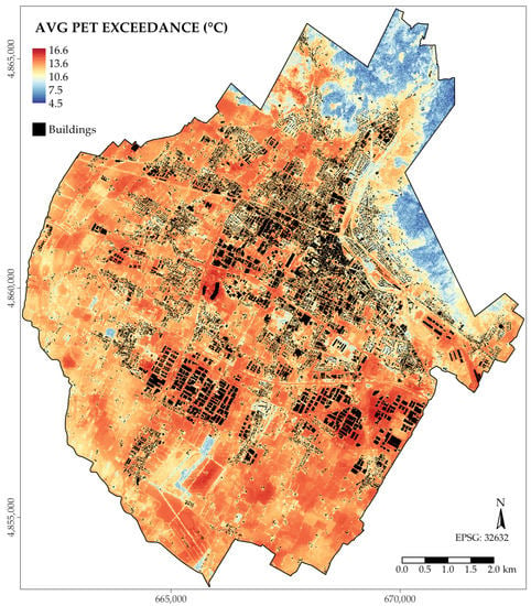
Figure 12.
Average (AVG) PET exceedance map for the study area.
PET exceedances zonal statistics according to land cover type are given in Table 6. The highest values were recorded for urban areas characterized by low VFC and high LST (presumably due to low albedo values), such as construction sites and industrial and commercial areas. High values were found also for rural areas characterized by high SVF such as meadows, crops and swamps. On the other hand, the lowest values were found for natural areas with low LST and SVF parameters (Table 2). It is interesting to note that during the day, the urban residential fabric, whether continuous or discontinuous, was characterized by low average PET exceedance values, certainly because of low SVF values (Table 2).

Table 6.
Average PET exceedances (°C) according to land cover class.
5. Discussion
In this study, we proposed a methodology to derive spatially and temporally resolved PET values at the city scale by combining remote sensing and meteorological data with Envi-met simulations. The Envi-met model [32] was selected since it delineates in a physical way the fluid dynamic, the radiation balance and its scattered components (both in short and long waves), the turbulent exchange fluxes, and the urban surface energy balance in complex environments such as urban areas. Therefore, simulations obtained with the Envi-met model are more physically based respect to other common software used for PET computation such as Rayman [29] or SkyHelios [30,31]. Even if Envi-met model implementation, as reported by Fröhlich and Matzarakis [30], has some shortcomings, the proposed methodology provides a new tool to overcome such limitations at urban scale. Moreover, this new method provided other advantages. Firstly, it proposed a system for spatializing hourly outcomes in a dynamic way using a proxy that depicts thermal patterns at different times of the day. This was obtained implementing the ECOSTRESS imagery (Table 4) within the calculation of the hUHTI index and setting specific time-dependent relationships between urban morphology and air temperature (Table 5). Until recently, the only high-resolution satellites able to provide surface temperature products were polar orbiting satellites (e.g., Landsat series) that acquire at a fixed daytime. By contrast, using ECOSTRESS imagery, the monitoring of surface thermal patterns at high resolution can nowadays be performed over different hours of the day. In addition, the hUHTI index, implementing urban morphology and degree of vegetation cover through the use of, respectively, SVF and NDVI, provided a more reliable characterization of human perceived thermal patterns and results indicated it as a more suitable tool as PET proxy compared to the sole remotely sensed LST product (Figure 8 and Table S5). Relationships between hUHTI and PET were generally stronger than those between LST and PET. The greater effectiveness of the hUHTI index as proxy of PET was particularly evident in the early morning and late afternoon, while around midday, coefficients of determination were analogue or slightly better for ECOSTRESS LST. This was probably due to the fact that around midday, the solar angle reaches its maximum value; therefore, shadows of buildings and trees are low, urban morphology has a lower weight on hUHTI calculation and, therefore, this last is more similar to LST than in other daytimes. On the contrary, linear relationships between LST and PET were weak and not statistically significant during the early (sunrise) and late (sunset) hours of the day; the reason was probably that LST alone, by measuring the top surface (e.g., roofs, etc.), was not able to depict phenomena characteristic of the hours preceding and following the night (heat release from impervious surfaces, atmospheric stability, vegetation that does not evapotranspirate) that, on the contrary, were effectively embedded in the hUHTI index.
Another advantage of the proposed methodology is the possibility to investigate daytime outdoor thermal patterns and trends despite the different acquisition dates that cover a relatively long period (end of June to mid-August). The selection of remotely sensed products acquired on dates coinciding with heatwave days (Table 1) and having overall similar meteorological characteristics (Table S4) allowed the investigation of diurnal thermal patterns and trends both at global study area level and in relation to its various land cover classes. The choice of analyzing an extreme event such as a heatwave obviously led to PET values of high thermal stress (above 35 °C) during the daytime, but the purpose of this investigation was to simulate the worst summer climatic scenario for the population in order to provide a tool for public administrations to intervene with urban regeneration plans in the most vulnerable areas.
Moreover, the results of the individual PET maps were summarized through the use of the PET exceedance map (Figure 12). The effectiveness of this type of map were already highlighted in the investigation by Koopmans et al. [51], which was related to a study area placed in the Netherlands. In this study, considering the different heatwave characteristics of the Prato study area, a slightly different approach was preferred (average exceedance > 35 °C vs. number of hours > 29 °C), but the advantages are the same, i.e., a synthetic product that can effectively support urban planners in the comprehension of PET patterns in urban, peri-urban and rural areas. For example, even if Brilli et al. [52] demonstrated, for the same study area, that the contribution of urban afforestation to the municipality carbon balance is low and carbon neutrality can only be reached by decarbonization of main emission sectors, the position of new urban trees with the respective de-sealing is an important instrument for urban planning. Tree dislocation may be optimized using the exceedance map to provide those substantial ecosystem services for the thermal and physiological wellbeing of the population with particular attention to the weakest groups [53]. In urban and peri-urban contexts, where space is scarce, an optimal solution could be the creation of pocket parks, while in a peri-urban context, along cycle-pedestrian routes, a solution may be the creation of microclimatic safety stops [54].
The methodology proposed in this study has some limitations both in data and method. Firstly, the method used for simple linear relationships establishment implicitly caused a simplification of urban PET patterns; part of the microclimate variability provided by the Envi-met modelling was lost using average values. However, as previously mentioned, this methodology aimed to provide a tool for stakeholders for urban planning and NBS intervention evaluation at city, neighborhood or block level; from this perspective, the loss of fluid dynamic details can be considered negligeable.
Another critical issue that emerged was the need for a sufficient number of weather stations for the characterization of the relationships between air temperature and remotely sensed parameters (LST, VFC and SVF). In the work by Nardino et al. [14], where UHTI was proposed and applied to the municipality of Bologna, this issue did not arise because there were five weather stations in the study area. In this study, however, only one weather station was available, thus hampering setting up relationships between air temperature and SVF and VFC parameters; consequently, for the first one, the linear relationship was established using air temperature data modeled with Envi-met, while for the second one, the relationship already calculated for Bologna in Nardino et al. [14] was applied. The implementation of this relationship not specific for the study area does not imply a study’s limitation, as the two cities (Prato and Bologna) are quite close (70 km), with similar climate and urban structure; moreover, Nardino et al. [14] demonstrated that VFC, among the three urban descriptors used for UHTI calculation, had the lowest percentage contribution.
The use of the ECOSTRESS imagery surely provides new opportunities for urban climate monitoring; previous studies [18,19] demonstrated how ECOSTRESS products are a valuable tool to detect and comprehend the environmental and anthropic factors affecting diurnal land surface thermal variations and patterns. In this investigation, the authors furnished another proof of the potentialities of this sensor since it was used to support the delineation of human perceived thermal patterns. However, it clearly emerged that the number of available scenes for a specific period or event (such as a heatwave) may vary considerably according to the unpredictable revisiting daytime of the ECOSTRESS sensor, the degree of cloud contamination, the frequent presence of data anomalies that were highlighted also in other investigations [21], thus hampering replicability of investigations. Moreover, the number of available scenes for the various diurnal phases may be unbalanced, as in this study, where the number of available ECOSTRESS scenes for the morning was almost double (five) compared to those available for the afternoon (three). Consequently, for a given study area, even the comparison between different years could be difficult since the available scenes could diverge significantly in number and regarding the acquisition daytime.
Regarding the results of the methodology applied to the Prato municipality, both PET Envi-met simulations and spatializations (Figure 5 and Figure 9) indicated that the resident population was severely affected during a heatwave by extreme heat stress, and since the first hours of the morning; only in green areas with dense tree cover the number of hours characterized by extreme heat stress was consistently lower. Regarding PET trends for the main types of urban fabric, the results (Figure 10 and Table S6) agreed with those of Nardino et al. [14]. The continuous residential fabric of the historical center (RACF) had lower PET values during the central diurnal hours compared to others such as the industrial and commercial areas (ICA). The reason was because UHTI and hUHTI indices embed the urban morphology through the SVF parameter and the SVF–Tair relationship. Specifically, SVF values in the historical center were generally lower than those in the industrial area (Table 2) due to a different urban structure characterized by narrow streets and relatively tall buildings. This condition could enhance shading effects, resulting in lower PET values. By the use of LST alone, the shadow effect cannot be evaluated since, in a densely built environment, the surface temperature measured by remotely sensed products was substantially relative to the roofs; therefore, the diurnal mitigating effect of the low SVF values linked to the narrow streets of the historical center was not detected. Regarding the industrial and commercial areas (ICA), which resulted characterized by the highest PET values, this result concurred with the investigation of Guerri et al. [55] on a study area (Florentine metropolitan area) that encompasses Prato municipality; the authors stated in their work that over 50% of industrial buildings fell into hot-spot areas due to high imperviousness and albedo levels and low presence of tree and grassland cover. An apparently surprising result was that green urban areas (GUA, Figure 10) had PET values slightly higher than the two types of residential urban fabric (RACF and RADSF). However, most of the urban parks in the study area were characterized by a low tree density with large meadows. Meadows, having high SVF and LST (Table 2) values, were characterized by high PET values (Table S6). Moreover, Prato urban green areas are generally small (average size = 1.18 ha), not irrigated and with rare little water areas; Liu et al. [20] recently demonstrated that the cooling effect of urban parks was positively correlated to its size, the presence of dense trees and water areas.
Finally, interesting results emerged regarding crops areas (C) that showed high PET values (Figure 10), similar to those of the industrial and commercial areas (ICA). This was primarily due to their high SVF values (Table 2), but it was also related to the phenological stage of the cultivations; in the study area, most of the crops (especially wheat), between the end of June and mid-August were at the end of their productive cycle and were, therefore, already harvested or in an advanced stage of ripening (LL and HL crop types of Figure 4). This implied very low values of evapotranspiration reflecting in low NDVI, factors that increased PET values. The ECOSTRESS and Sentinel 2 scenes used in this study covered a fairly large period of time (i.e., end of June to mid-August); therefore, the hourly PET values of the agricultural areas were likely influenced by the phenological stage of the crops. This aspect was clearly highlighted in Figure 11, where hourly PET values of different crops were related to the acquisition date of the remotely sensed products used for hUHTI calculation. Overall, these results suggest the investigation of the thermal effect of peri-urban crops on urban areas; for example, large crops at the end of their productive cycle could negatively affect the nearby urban areas, especially during heatwaves, with a role practically opposite to that of large densely wooded urban green areas.
6. Conclusions
In this work, a methodology to spatialize Envi-met modelled test areas PET values over a whole study area was presented; the method took advantage of the daytime temporal patterns detected by hUHTI, a modified version of the UHTI index that implements ECOSTRESS imagery. A case study relating to the municipal area of the city of Prato (central Italy) was presented; thermal patterns according to land cover class were temporally and spatially investigated, allowing to identify the grade of thermal discomfort in each sub-area. Despite the method’s limitations mentioned above, the spatialization of the PET obtained from an up-scaling of the Envi-met fluid dynamic model allows to provide valuable information to public administrations and stakeholders at city scale, especially in terms of urban regeneration. Future research plans to integrate this hazard information with geospatial fragility, adaptation and exposure data to map and evaluate heatwave related risk. This action will lead to an operational tool for the implementation of concrete actions intervening primarily in the areas most at risk for the most fragile sections of the population.
Supplementary Materials
The following supporting information can be downloaded at: https://www.mdpi.com/article/10.3390/atmos14040641/s1, Table S1: Physiological Equivalent Temperature (PET) for different grades of thermal sensation and physiological stress on human beings during standard conditions (internal heat production: 80 W, heat transfer resistance of the clothing: 0.9 clo) for Western/Middle Europe (after Matzarakis and Mayer, 1996); Table S2: Selected ECOSTRESS LST scenes used in this study; Table S3: Sentinel 2 scenes used in this study; Table S4: Meteorological characteristics of the selected days for hUHTI calculation (AVG = average; NA = not available); Table S5: Simple linear regression metrics of hUHTI and LST and PET Envi-met modelling outputs (* = p value ≤ 0.05; ** = p value ≤ 0.01; *** = p value ≤ 0.001); Table S6: Mean PET values at different daytimes according to land cover class.
Author Contributions
Conceptualization, E.F. and M.N.; methodology, E.F. and M.N.; software, E.F., L.C. and M.N.; validation, E.F. and M.N.; formal analysis, E.F., L.C. and M.N.; investigation, E.F. and M.N.; resources, E.F. and M.N.; data curation, E.F. and M.N.; writing—original draft preparation, E.F. and M.N.; writing—review and editing, E.F., F.C., L.B., T.G., L.C., B.G. and M.N.; visualization, E.F.; supervision, E.F.; project administration, B.G.; funding acquisition, B.G. All authors have read and agreed to the published version of the manuscript.
Funding
This research was funded by the Urban Innovative Action Program (UIA) of the European Union., grant number UIA04-176 PUJ.
Institutional Review Board Statement
Not applicable.
Informed Consent Statement
Not applicable.
Data Availability Statement
Data sharing is not applicable to this article.
Acknowledgments
The authors want to thank Giovanni Nerini, Antonietta Perretta and Pamela Bracciotti (Prato Municipality) for providing municipality related datasets. The authors are also grateful to the four anonymous reviewers for their helpful comments and notes.
Conflicts of Interest
The authors declare no conflict of interest.
References
- Santamouris, M. Energy and Climate in the Urban Built Environment; Routledge: New York, NY, USA, 2013; ISBN 9781134257904. [Google Scholar]
- Learn About Heat Islands. Available online: https://www.epa.gov/heatislands/learn-about-heat-islands (accessed on 8 November 2022).
- Jamei, E.; Rajagopalan, P.; Seyedmahmoudian, M.; Jamei, Y. Review on the Impact of Urban Geometry and Pedestrian Level Greening on Outdoor Thermal Comfort. Renew. Sustain. Energy Rev. 2016, 54, 1002–1017. [Google Scholar] [CrossRef]
- Zuo, J.; Pullen, S.; Palmer, J.; Bennetts, H.; Chileshe, N.; Ma, T. Impacts of Heat Waves and Corresponding Measures: A Review. J. Clean. Prod. 2015, 92, 1–12. [Google Scholar] [CrossRef]
- Woolley, H. Urban Open Spaces; Taylor & Francis: Abingdon, UK, 2003; ISBN 9781135802295. [Google Scholar]
- Peng, S.; Piao, S.; Ciais, P.; Friedlingstein, P.; Ottle, C.; Bréon, F.-M.; Nan, H.; Zhou, L.; Myneni, R.B. Surface Urban Heat Island Across 419 Global Big Cities. Environ. Sci. Technol. 2012, 46, 696–703. [Google Scholar] [CrossRef] [PubMed]
- Sheng, L.; Tang, X.; You, H.; Gu, Q.; Hu, H. Comparison of the Urban Heat Island Intensity Quantified by Using Air Temperature and Landsat Land Surface Temperature in Hangzhou, China. Ecol. Indic. 2017, 72, 738–746. [Google Scholar] [CrossRef]
- Hu, L.; Brunsell, N.A. The Impact of Temporal Aggregation of Land Surface Temperature Data for Surface Urban Heat Island (SUHI) Monitoring. Remote Sens. Environ. 2013, 134, 162–174. [Google Scholar] [CrossRef]
- Gallo, K.; Hale, R.; Tarpley, D.; Yu, Y. Evaluation of the Relationship between Air and Land Surface Temperature under Clear- and Cloudy-Sky Conditions. J. Appl. Meteorol. Climatol. 2011, 50, 767–775. [Google Scholar] [CrossRef]
- Good, E.J.; Ghent, D.J.; Bulgin, C.E.; Remedios, J.J. A Spatiotemporal Analysis of the Relationship between Near-surface Air Temperature and Satellite Land Surface Temperatures Using 17 Years of Data from the ATSR Series. J. Geophys. Res. Atmos. 2017, 122, 9185–9210. [Google Scholar] [CrossRef]
- Huang, W.; Li, J.; Guo, Q.; Mansaray, L.; Li, X.; Huang, J. A Satellite-Derived Climatological Analysis of Urban Heat Island over Shanghai during 2000–2013. Remote Sens. 2017, 9, 641. [Google Scholar] [CrossRef]
- Agathangelidis, I.; Cartalis, C.; Santamouris, M. Estimation of Air Temperatures for the Urban Agglomeration of Athens with the Use of Satellite Data. Geoinformatics Geostat. Overv. 2016, 4, 2. [Google Scholar] [CrossRef]
- Dos Santos, R.S. Estimating Spatio-Temporal Air Temperature in London (UK) Using Machine Learning and Earth Observation Satellite Data. Int. J. Appl. Earth Obs. Geoinf. 2020, 88, 102066. [Google Scholar] [CrossRef]
- Nardino, M.; Cremonini, L.; Crisci, A.; Georgiadis, T.; Guerri, G.; Morabito, M.; Fiorillo, E. Mapping Daytime Thermal Patterns of Bologna Municipality (Italy) during a Heatwave: A New Methodology for Cities Adaptation to Global Climate Change. Urban Clim. 2022, 46, 101317. [Google Scholar] [CrossRef]
- Pichierri, M.; Bonafoni, S.; Biondi, R. Satellite Air Temperature Estimation for Monitoring the Canopy Layer Heat Island of Milan. Remote Sens. Environ. 2012, 127, 130–138. [Google Scholar] [CrossRef]
- Vulova, S.; Meier, F.; Fenner, D.; Nouri, H.; Kleinschmit, B. Summer Nights in Berlin, Germany: Modeling Air Temperature Spatially with Remote Sensing, Crowdsourced Weather Data, and Machine Learning. IEEE J. Sel. Top. Appl. Earth Obs. Remote Sens. 2020, 13, 5074–5087. [Google Scholar] [CrossRef]
- Chang, Y.; Xiao, J.; Li, X.; Zhou, D.; Wu, Y. Combining GOES-R and ECOSTRESS Land Surface Temperature Data to Investigate Diurnal Variations of Surface Urban Heat Island. Sci. Total Environ. 2022, 823, 153652. [Google Scholar] [CrossRef]
- Chang, Y.; Xiao, J.; Li, X.; Middel, A.; Zhang, Y.; Gu, Z.; Wu, Y.; He, S. Exploring Diurnal Thermal Variations in Urban Local Climate Zones with ECOSTRESS Land Surface Temperature Data. Remote Sens. Environ. 2021, 263, 112544. [Google Scholar] [CrossRef]
- Hulley, G.; Shivers, S.; Wetherley, E.; Cudd, R. New ECOSTRESS and MODIS Land Surface Temperature Data Reveal Fine-Scale Heat Vulnerability in Cities: A Case Study for Los Angeles County, California. Remote Sens. 2019, 11, 2136. [Google Scholar] [CrossRef]
- Liu, Y.; Xu, X.; Wang, F.; Qiao, Z.; An, H.; Han, D.; Luo, J. Exploring the Cooling Effect of Urban Parks Based on the ECOSTRESS Land Surface Temperature. Front. Ecol. Evol. 2022, 10, 1031517. [Google Scholar] [CrossRef]
- Wang, Q.; Wang, X.; Meng, Y.; Zhou, Y.; Wang, H. Exploring the Impact of Urban Features on the Spatial Variation of Land Surface Temperature within the Diurnal Cycle. Sustain. Cities Soc. 2023, 91, 104432. [Google Scholar] [CrossRef]
- Binarti, F.; Koerniawan, M.D.; Triyadi, S.; Utami, S.S.; Matzarakis, A. A Review of Outdoor Thermal Comfort Indices and Neutral Ranges for Hot-Humid Regions. Urban Clim. 2020, 31, 100531. [Google Scholar] [CrossRef]
- Chen, L.; Ng, E. Outdoor Thermal Comfort and Outdoor Activities: A Review of Research in the Past Decade. Cities 2012, 29, 118–125. [Google Scholar] [CrossRef]
- Zhao, Q.; Lian, Z.; Lai, D. Thermal Comfort Models and Their Developments: A Review. Energy Built Environ. 2021, 2, 21–33. [Google Scholar] [CrossRef]
- Matzarakis, A.; Mayer, H.; Iziomon, M.G. Applications of a Universal Thermal Index: Physiological Equivalent Temperature. Int. J. Biometeorol. 1999, 43, 76–84. [Google Scholar] [CrossRef] [PubMed]
- Matzarakis, A.; Endler, C. Climate Change and Thermal Bioclimate in Cities: Impacts and Options for Adaptation in Freiburg, Germany. Int. J. Biometeorol. 2010, 54, 479–483. [Google Scholar] [CrossRef] [PubMed]
- Höppe, P. The Physiological Equivalent Temperature—A Universal Index for the Biometeorological Assessment of the Thermal Environment. Int. J. Biometeorol. 1999, 43, 71–75. [Google Scholar] [CrossRef]
- Matzarakis, A.; Mayer, H. Another Kind of Environmental Stress: Thermal Stress. WHO Collab. Cent. Air Qual. Manag. Air Pollut. Control. Newsl. 1996, 18, 7–10. [Google Scholar]
- Matzarakis, A.; Rutz, F.; Mayer, H. Modelling Radiation Fluxes in Simple and Complex Environments: Basics of the RayMan Model. Int. J. Biometeorol. 2010, 54, 131–139. [Google Scholar] [CrossRef]
- Fröhlich, D.; Matzarakis, A. Spatial Estimation of Thermal Indices in Urban Areas-Basics of the Skyhelios Model. Atmosphere 2018, 9, 209. [Google Scholar] [CrossRef]
- Matzarakis, A.; Gangwisch, M.; Fröhlich, D. RayMan and SkyHelios Model. In Urban Microclimate Modelling for Comfort and Energy Studies; Palme, M., Salvati, A., Eds.; Springer International Publishing: Cham, Switzerland, 2021; pp. 339–361. ISBN 978-3-030-65421-4. [Google Scholar]
- Bruse, M.; Fleer, H. Simulating Surface–Plant–Air Interactions inside Urban Environments with a Three Dimensional Numerical Model. Environ. Model. Softw. 1998, 13, 373–384. [Google Scholar] [CrossRef]
- Liu, Z.; Cheng, W.; Jim, C.Y.; Morakinyo, T.E.; Shi, Y.; Ng, E. Heat Mitigation Benefits of Urban Green and Blue Infrastructures: A Systematic Review of Modeling Techniques, Validation and Scenario Simulation in ENVI-Met V4. Build. Environ. 2021, 200, 107939. [Google Scholar] [CrossRef]
- Tsoka, S.; Tsikaloudaki, A.; Theodosiou, T. Analyzing the ENVI-Met Microclimate Model’s Performance and Assessing Cool Materials and Urban Vegetation Applications–A Review. Sustain. Cities Soc. 2018, 43, 55–76. [Google Scholar] [CrossRef]
- Yang, X.; Zhao, L.; Bruse, M.; Meng, Q. Evaluation of a Microclimate Model for Predicting the Thermal Behavior of Different Ground Surfaces. Build. Environ. 2013, 60, 93–104. [Google Scholar] [CrossRef]
- Kottek, M.; Grieser, J.; Beck, C.; Rudolf, B.; Rubel, F. World Map of the Köppen-Geiger Climate Classification Updated. Meteorol. Z. 2006, 15, 259–263. [Google Scholar] [CrossRef] [PubMed]
- Consorzio LaMMA. Available online: http://www.lamma.rete.toscana.it/ (accessed on 20 November 2022).
- Magno, R.; De Filippis, T.; Di Giuseppe, E.; Pasqui, M.; Rocchi, L.; Gozzini, B. Semi-Automatic Operational Service for Drought Monitoring and Forecasting in the Tuscany Region. Geosciences 2018, 8, 49. [Google Scholar] [CrossRef]
- Ondate Di Calore—Ministero Della Salute. Available online: https://www.salute.gov.it/portale/caldo/homeCaldo.jsp (accessed on 20 November 2022).
- Guattari, C.; Evangelisti, L.; Balaras, C.A. On the Assessment of Urban Heat Island Phenomenon and Its Effects on Building Energy Performance: A Case Study of Rome (Italy). Energy Build. 2018, 158, 605–615. [Google Scholar] [CrossRef]
- Copernicus Open Access Hub. Available online: https://scihub.copernicus.eu (accessed on 20 November 2022).
- Rouse, J.; Haas, R.; Schell, J.; Deering, D. Monitoring Vegetation Systems in the Great Plains with ERTS. In Proceedings of the 3rd Earth Resources Technology Satellite-1 Symposium, Washington, DC, USA, 10–14 December 1973; Technical Presentations. NASA SP-351: Washington, DC, USA, 1974; Volume 1, pp. 309–317. [Google Scholar]
- Qi, J. Spatial and Temporal Dynamics of Vegetation in the San Pedro River Basin Area. Agric. For. Meteorol. 2000, 105, 55–68. [Google Scholar] [CrossRef]
- Oke, T.R. Canyon Geometry and the Nocturnal Urban Heat Island: Comparison of Scale Model and Field Observations. J. Climatol. 1981, 1, 237–254. [Google Scholar] [CrossRef]
- Toscana Geoportal. Available online: https://dati.toscana.it/dataset/ucs (accessed on 20 November 2022).
- QGIS Software. Available online: https://www.qgis.org/en/site/ (accessed on 20 November 2022).
- R Software. Available online: https://www.r-project.org/ (accessed on 20 November 2022).
- Stewart, I.D.; Oke, T.R. Local Climate Zones for Urban Temperature Studies. Bull. Am. Meteorol. Soc. 2012, 93, 1879–1900. [Google Scholar] [CrossRef]
- International Standard Organization ISO 7730: Ergonomics of the Thermal Environment Analytical Determination and Interpretation of Thermal Comfort Using Calculation of the PMV and PPD Indices and Local Thermal Comfort Criteria. Management 2005, 3, 605–615.
- MacQueen, J. Some Methods of Classification and Analysis of Multivariate Observation. In Proceedings of the Fifth Berkeley Symposium on Mathematical Statistics and Probability University of California, Los Angeles, CA, USA, 21 June–8 July 1965, 27 December 1965–7 January1966; pp. 281–297. [Google Scholar]
- Koopmans, S.; Heusinkveld, B.G.; Steeneveld, G.J. A Standardized Physical Equivalent Temperature Urban Heat Map at 1-m Spatial Resolution to Facilitate Climate Stress Tests in the Netherlands. Build. Environ. 2020, 181, 106984. [Google Scholar] [CrossRef]
- Brilli, L.; Carotenuto, F.; Chiesi, M.; Fiorillo, E.; Genesio, L.; Magno, R.; Morabito, M.; Nardino, M.; Zaldei, A.; Gioli, B. An Integrated Approach to Estimate How Much Urban Afforestation Can Contribute to Move towards Carbon Neutrality. Sci. Total Environ. 2022, 842, 156843. [Google Scholar] [CrossRef]
- Guolo, F.; Stivanello, E.; Pizzi, L.; Georgiadis, T.; Cremonini, L.; Musti, M.A.; Nardino, M.; Ferretti, F.; Marzaroli, P.; Perlangeli, V.; et al. Emergency Department Visits and Summer Temperatures in Bologna, Northern Italy, 2010–2019: A Case-Crossover Study and Geographically Weighted Regression Methods. Int. J. Environ. Res. Public Health 2022, 19, 5592. [Google Scholar] [CrossRef] [PubMed]
- Cremonini, L.; Nardino, M.; Georgiadis, T. The Utilization of the WMO-1234 Guidance to Improve Citizen’s Wellness and Health: An Italian Perspective. Int. J. Environ. Res. Public Health 2022, 19, 5056. [Google Scholar] [CrossRef] [PubMed]
- Guerri, G.; Crisci, A.; Congedo, L.; Munafò, M.; Morabito, M. A Functional Seasonal Thermal Hot-Spot Classification: Focus on Industrial Sites. Sci. Total Environ. 2022, 806, 151383. [Google Scholar] [CrossRef] [PubMed]
Disclaimer/Publisher’s Note: The statements, opinions and data contained in all publications are solely those of the individual author(s) and contributor(s) and not of MDPI and/or the editor(s). MDPI and/or the editor(s) disclaim responsibility for any injury to people or property resulting from any ideas, methods, instructions or products referred to in the content. |
© 2023 by the authors. Licensee MDPI, Basel, Switzerland. This article is an open access article distributed under the terms and conditions of the Creative Commons Attribution (CC BY) license (https://creativecommons.org/licenses/by/4.0/).
