Article

Comparative Study on the Use of Some Low-Cost Optical Particulate Sensors for Rapid Assessment of Local Air Quality Changes

1
Department of Applied and Nonlinear Optics, Institute for Solid State Physics and Optics, Wigner Research Centre for Physics, P.O. Box 49, H-1525 Budapest, Hungary
2
Plósz Engineering Office Ltd., KFKI-Campus, Konkoly-Thege Miklós út 29-33, H-1121 Budapest, Hungary
3
Department of Science and Laboratory Technology, Dar es Salaam Institute of Technology, Dar es Salaam P.O. Box 2958, Tanzania
4
Department of Analytical Chemistry, Institute of Chemistry, Loránd Eötvös University, Pázmány Péter Sétány 1/a, H-1117 Budapest, Hungary
*
Author to whom correspondence should be addressed.
Atmosphere 2022, 13(8), 1218; https://doi.org/10.3390/atmos13081218
Submission received: 13 July 2022 / Accepted: 26 July 2022 / Published: 2 August 2022
(This article belongs to the Section Atmospheric Techniques, Instruments, and Modeling)

Abstract

:
Official air quality (AQ) stations are sporadically located in cities to monitor the anthropogenic pollutant levels. Consequently, their data cannot be used for further locations to estimate hidden changes in AQ and local emissions. Low-cost sensors (LCSs) of particulate matter (PM) in a network can help in solving this problem. However, the applicability of LCSs in terms of analytical performance requires careful evaluation. In this study, two types of pocket-size LCSs were tested at urban, suburban and background sites in Budapest, Hungary, to monitor PM1, PM2.5, PM10, and microclimatic parameters at high resolutions (1 s to 5 min). These devices utilize the method of laser irradiation and multi-angle light scattering on air-suspended particulates. A research-grade AQ monitor was applied as a reference. The LCSs showed acceptable accuracy for PM species in indoor/outdoor air even without calibration. Low PM readings (<10 μg/m3) were generally handicapped by higher bias, even between sensors of the same type. The relative humidity (RH) slightly affected the PM readings of LCSs at RHs higher than 85%, necessitating field calibration. The air quality index was calculated to classify the extent of air pollution and to make predictions for human health effects. The LCSs were useful for detecting peaks stemming from emissions of motor vehicular traffic and residential cooking/heating activities.

1. Introduction

Anthropogenic pollution in ambient air, especially in the form of suspended particulate matter (PM), is of general concern worldwide, due to its negative effects on human health [1], global climate change [2], and various buildings related to cultural heritage preservation [3]. Besides these, high levels of outdoor air pollution can trigger bad indoor air quality, deteriorating people’s comfort and health [4]. Consequently, the degree of anthropogenic pollution in terms of the detection and identification of air components as well as their concentrations and size distributions should be monitored with as high a spatial and temporal resolution as possible, to reveal the hidden atmospheric processes of pollution episodes.
Official (e.g., state-sustained) air quality (AQ) stations are in general sparsely located in city and provincial sites of Hungary, which is true for most of other countries worldwide as well. In this sense, in populated areas situated further from these air quality stations, using their monitor data, it is difficult, and in general highly biased, to assess the changes in local emissions and pollutant levels, stemming, for instance, from intensified motor vehicle traffic, wood/coal-based heating, and/or biomass burning activities. For this type of estimation, atmospheric air pollution dispersion models play a supportive role, providing high-resolution concentration maps of aerosols [5]. On the other hand, the application of the complex atmospheric pollution models demands knowledge on the exact environmental variables of air quality and weather parameters for the area of interest to be as detailed as possible to approach/calculate local air quality scenarios with good accuracy and to make predictions on changes of air quality as well as PM deposition [5]. Extended measurement networks based on low-cost sensors (LCSs) for air quality, commercially available to the population at large, can help in solving the above addressed problem and can provide datasets detailed enough for checking official air quality legislation and for providing the necessary input data for atmospheric dispersion models of high resolution as well.
So far, several methods have been reported in the relevant literature, dealing with the extension of air quality network/nodes by the use of commercial sensors [6,7,8,9,10,11,12,13,14,15,16,17,18,19,20,21,22]. For example, Moltchanov et al. [6] demonstrated the feasibility of an air quality network to capture the spatio-temporal concentration variations with exceptionally high resolution, but they also highlighted the need for frequent in situ calibration of each node to maintain the consistent reading of the sensors, for which they developed a procedure, based on mathematical correction.
Jerret et al. [7] validated low-cost, personal AQ sensors for CO, NO and NO2 to reduce exposure measurement errors in epidemiological studies and compared their data with those obtained from more costly governmental instruments. They observed moderate-to-high correlations for NO and CO, but low-to-moderate correlations for NO2. Mead et al. [8] applied miniature electrochemical LCSs in a high-density network for monitoring urban gaseous pollutant levels at ppb mixing ratios in Cambridge, UK. These systems allowed the deployment of a high-density AQ sensor network with high spatial and temporal scales, and in static (wider Cambridge area) and mobile (e.g., personal exposure) configurations.
Castell et al. [9] evaluated 24 units of a commercial LCS platform (AQMesh) for the measurement of CO, NO, NO2, and O3 against official reference analyzers (CEN—European Standardization Organization). The analytical performance of the LCSs changed from unit to unit, spatially and temporally, depending on the atmospheric composition and meteorological conditions, which demanded a necessary scrutiny of measurement data of each node, before monitoring application.
Thorpe and Walsh [10] compared the performance of portable, real-time dust monitors (SKC Split 2, Microdust Pro, DataRam) inside a calm air dust chamber using industrial and aluminum oxides as model dusts. The response of the monitors to respirable PM was linear when operating the sampler either passively or actively with cyclone inlets. They observed a lower response when operated actively, as compared to the passive operation, and still lower when used with porous foam inserts. Inhalable dust measured with Split 2 agreed closely with reference IOM inhalable samplers, whereas the Microdust CIS-adaptor underestimated the inhalable PM concentration compared to the reference.
In another study, Salimifard et al. [11] investigated the performance of low-cost optical particle counters (OPCs) (OPC-N2, Alphasense Ltd., Essex, UK; IC Sentinel, Speck, Dylos) in monitoring individual aerosols that were commonly found indoors in a controlled chamber environment. Biological (dust mite, pollen, cat, and dog fur) and non-biological (monodisperse silica, melamine resin) particulate was applied for exposure studies in the aerosol chamber. The PM concentration had the most dominant effect on the linearity of the sensors’ response, whereas the particle size and type had a lower influence on it.
Hagan et al. [12] applied an integrated multi-pollutant LCS system and a co-located research-grade instrument for characterizing gaseous and particulate pollution sources in Delhi, India, for six weeks in winter. They utilized non-negative matrix factorization to deconvolve the sensor data into unique factors that were identified after then by using the factor composition of measurements extracted from the data of the research-grade monitor. They found three factors: one combustion related, showing high levels of CO and two characterized by the sampled PM. The important goal of their work was to show that by multipollutant LCS monitoring—despite the instrumental restrictions of these devices—one can obtain insight into sources of fine PM in urban environments.
Oluwadairo et al. [13] tested LCSs for PM2.5 in urban environments with different road traffic conditions in Houston, Texas, and observed linear relationship of the monitoring data with those from research-grade instruments. The regression slopes and coefficients differed across the investigated environments, whereas the mean bias was similar. They concluded that the use of correct slopes of LCS calibration was key for attaining accurate PM2.5 readings in an urban environment. Wahlborg et al. [14] applied AQMesh type AQ monitor for field calibration of NO, NO2 and PM10 species in summer and autumn campaigns in a busy street in the mid-size city of Gävle, Sweden. By means of linear calibration methods (i.e., post-scaled, bisquare, and orthogonal), they attained more accurate results compared to the raw monitoring data. These improvements were sufficient to satisfy the EU Data Quality Objective for indicative measurements during the autumn period. The bisquare procedure improved the root mean square error by the same extent as other studies using complex multivariate calibration methods.
Crilley et al. [
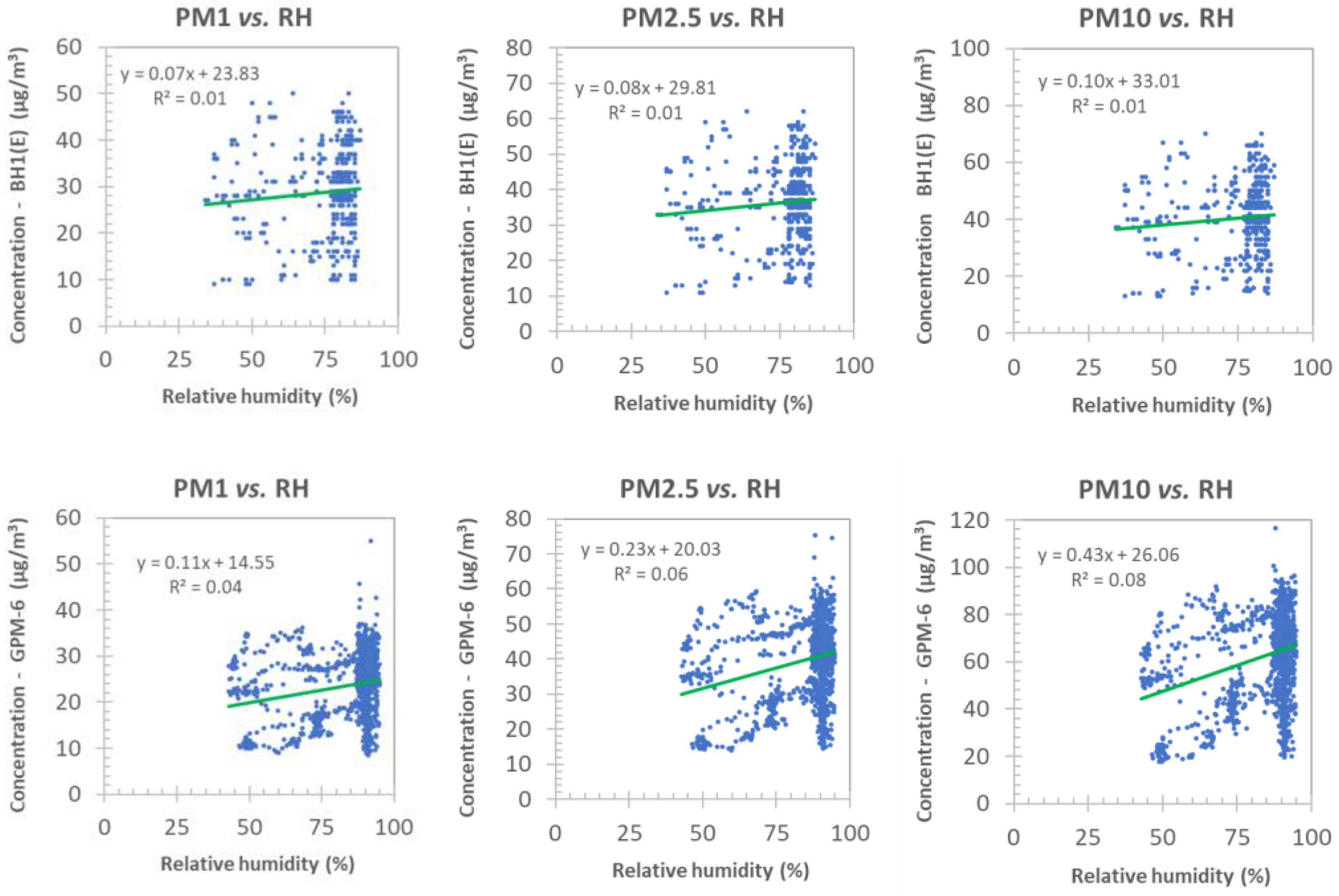
15] evaluated, on field, the OPC-N2 for monitoring ambient PM on urban background sites in the UK. This sensor demonstrated a significant positive artefact in particle mass during events of high ambient relative humidity (RH) (>85%) when compared to reference OPCs and TEOM-FDMS. Therefore, the authors suggested a calibration factor for OPC-N2, which was developed based on the κ-Köhler theory, using average bulk particle aerosol hygroscopicity. This factor increased the accuracy to within 33% of that of TEOM-FDMS. The precision for 14 OPC-N2 sensors was 22 ± 13% for PM10.
Yuval et al. [16] applied a network of OPCs, in a year-long campaign of continuous measurements of particle number concentration (PNC) in a couple of locations in Elad, Israel, and its vicinity, to assess the influence of a close quarry on the AQ of the city. They investigated the OPCs’ accuracy, coherency, and capability to detect the quarry’s impact on the urban PNC levels. Using temporal PNC series in two-size channels from a network of five nodes, PM2.5 and PM10 records from a nearby reference AQ station, and meteorological data, they found a low impact of the quarry on the city, as compared to the background PNC. They also demonstrated the use of a network of low-cost OPCs for responding to an environmental issue for which the sparse standard AQ monitoring observations were found to be insufficient.
Markowicz and Chiliński [17] studied co-located OPCs (Dfrobot SEN0177 and OPC-N2) for the determination of the aerosol scattering coefficient (ASC) and Ångström exponent (AE), which are important in understanding aerosol optical properties and their direct effects. For PM10, the ASC function was found to be linear with strong correlation for Dfrobot and non-linear for OPC-N2, each providing the ASC with similar difference: ≈27% of the mean value. Interestingly, the relative measurement uncertainty was independent of the PM level. Moreover, the ratio of PNC between different bins showed a significant correlation (at 95% confidence level) with the scattering AE. Comparisons of an estimated scattering AE from a low-cost sensor with the reference instrument of Aurora 4000 were given with a mean square error of 0.23–0.24, corresponding to 16–19% deviation.
Sousan et al. [18] demonstrated the application of four LCSs (OPC-N3, SPS30, AirBeam2 and PMS A003) and calibration differences between environmental and occupational settings. The air levels of salt, road dust, and oil were measured and compared with a reference instrument. They found OPC-N2 and SPS30 to be highly correlated with the reference device for each aerosol type in the environmental settings. In occupational settings, only the data of OPC-N3 showed variation. The bias varied by particle size and aerosol type. The SPS30 and OPC-N3 sensors were characterized by a low bias for environmental settings. On the other hand, each studied sensor showed a high bias for occupational settings. The findings suggest that SPS20 and OPC-N3 can provide a reasonable estimate of air PM levels, providing that they are calibrated for either environmental or occupational settings using apt site-specific factors. Huang and co-workers [19] also studied Air-Beam2 sensors in urban offices, a mass-transit railway station (platform and lobby), and at the seaside, using TSI DustTrak DRX monitor as a reference. High linearity between the data of the LCSs and the reference monitor was observed using various measurement cycles (5 s to 30 min). Weather conditions affected the accuracy and bias of the sensor readings, especially during rainy days, and/or fog/high-RH events. Sampling sites with a high hygroscopic salt content of the PM (e.g., seaside) experienced similar behavior. The machine learning procedure, Random Forest, was found to be advantageous over multiple linear regression for PM data calibration on days without rain.
Wang et al. [20] investigated the analytical performance of three kinds of LCSs—PPD42NS, DSM501A, and GP2Y110AU0F—against various reference instruments, following US EPA 2013 recommendations for the evaluation of the performance of the LCSs. They also observed the effects of climatic parameters, PM size and concentration important to the linearity of the monitor data. Jayaratne et al. [21] and Sayahi et al. [22] reported similar findings on the effect of high ambient RH on PM readings of LCSs using PMS-type devices. Besides the above summarized studies, reviews from recent years extensively discussed the peculiarities of LCSs for air PM monitoring purposes [23,24,25].
As it comes from the above overview, the accurate response of low-cost sensors to local air pollution is not obvious. In general, broad assessment of the analytical performance, often involving field calibration/resloping, is necessary to obtain accurate readings from these types of field-deployable devices. Consequently, in this study, we have evaluated the performance of two types of pocket-sized, low-cost air quality sensors, which have not yet been studied in the relevant literature. For monitoring purposes, we selected three sites of different anthropogenic influence in Budapest, Hungary. The resultant PM data series were compared and statistically evaluated on the base of each monitoring node outdoors and indoors. Moreover, some predictions for health effects were made based on the air quality index (AQI) and following the recommendation of US EPA.

2. Materials and Methods

2.1. Description of the Sampling Sites

Three sites of different anthropogenic impacts in Budapest, Hungary, have been selected and used for sampling the ambient air and collecting air quality data. These sites represent urban, suburban, and background locations regarding air pollution. The first sampling site (geocoordinates: 47°26′39.40″ N, 19°07′11.51″ E) is in Pesterzsébet, which is a district on outskirts of Budapest. The site is a typical urban location with residential houses and gardens, in general, with medium traffic density, due to nearby main roads. There are some anthropogenic activities in nearby car/mechanical workshops. In winter, the heating is based on wood/fossil fuel, favored by the local population. The outdoor sampling spot was chosen in a dwelling house, located about 15 m along a main road, with its front garden with several pine trees and bushes providing a kind of shield against traffic-released PM. At this site, the anteroom (area: ≈12 m2, opening to a garden, a kitchen, and a hall) and the living room (area: ≈20 m2) were used for indoor air sampling. The second sampling site is situated in a suburban area (geocoordinates: 47°32′48.63″ N, 18°58′2.79″ E) close to a large forest in the Buda hills, in the district of Hűvösvölgy (“Cool Valley” in Hungarian). This site is at the farther side of a dead-end street, about 200 m from the closest major road, thus possessing a very low density of local motor vehicular traffic. Due to the proximity of the forest, the ambient air of this site is frequently refreshed.
The third sampling site has been selected to be at one of the buildings of the Wigner Research Centre for Physics (KFKI Campus), which is situated in the Buda hills (geocoordinates: 47°29′26.51″ N, 18°57′22.13″ E), but much farther from the former sampling point. This site is characterized by a low anthropogenic impact considering the low density of traffic and negligible industrial activities. This location can be the best described as an urban background site. The campus’ buildings are located amongst the trees of the forest, which surround the area and provide fresh air. The anthropogenic pollution activity in this area can be characterized by some emissions from its own gaseous-based heating center in winter, the low-frequency of local motor vehicular traffic including personal cars, and at the end station, of one bus line on the opposite side to the main gates, as well as two kitchens for the on-site cafeterias and some low-emission activities of chemical–physical research, a car repair shop, and general workshops, causing only low emissions of gases and aerosols (e.g., by releasing welding fumes). At this site, the indoor sampling was performed in one of the offices (area: 15 m2), equipped with regular furniture (e.g., a couple of desks and bookshelves).

2.2. Instrumentation

In the present study, low-cost PM monitors of the Geekcreit® (China) model PM1.0/PM2.5/PM
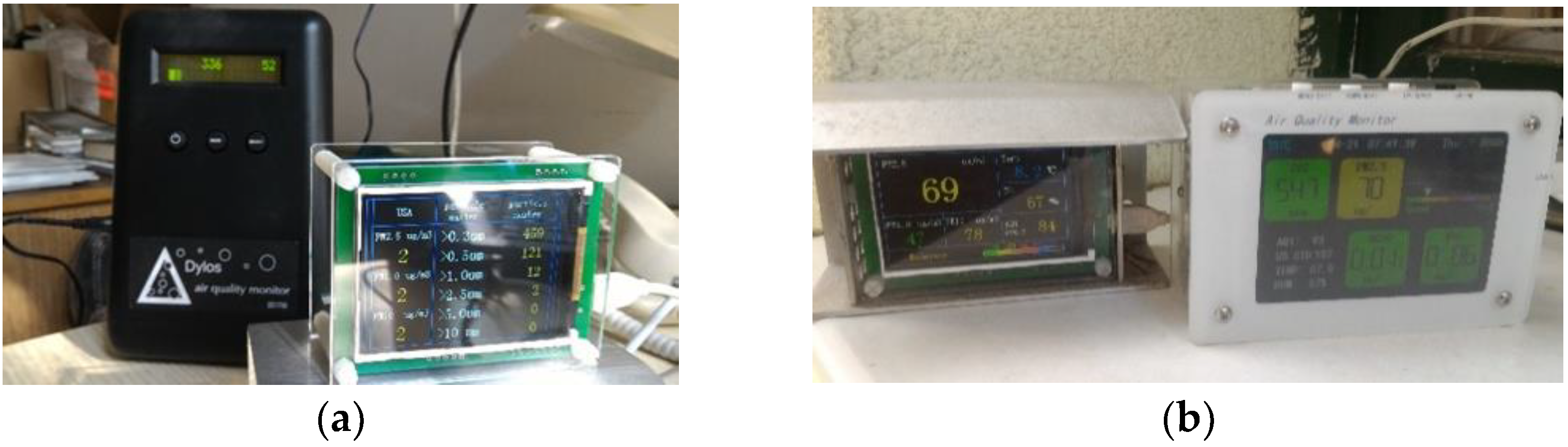
10, based on a PMS5003 Plantower PM sensor (herein referred to as “GPM sensor”), and Bohu Model BH1 (Bohu-Tech, China) were purchased and applied for daily aerosol monitoring. Both types of sensors are lightweight (GPM: 118 g, but 270 g with Al-housing, BH1: 324 g) and cost about USD 45 and USD 220, respectively. These devices utilize the method of continuous air sampling, laser irradiation, and multi-angle light scattering on air-suspended particulate. In brief, according to the intensity and angle of the scattered light, temporally varying curves can be recorded, which are processed by the built-in 32-bit microcomputer. The results are obtained as equivalent aerodynamic particle diameters, and the number of suspended PM with different sizes in a unit volume of air can be obtained. For indoor air monitoring, the LCSs were used as purchased. For outdoor purposes, the BH1 sensors were placed under rain shelters. Additionally, the GPM sensors were equipped with a supportive, closed aluminum housing to prevent the ingress of daily precipitation and/or soil dust by wind throughout the open parts of the device (Figure 1). With this housing, a hard plastic wall was also built in between the flow inlet and outlet to prevent internal mixing of the sampled air. To assure the accurate readings for PM, the performance of each housed LCS unit was tested against non-housed devices of the same type. The monitors were placed at least 1.5 m (outdoors) and 1.2 m (indoors) above the ground, and about 0.4 m from the walls of the buildings. The distance of the monitors from each other was about 0.2–0.3 m at every sampling spot.
For air quality monitoring, PM1, PM2.5, and PM10 were sampled with a resolution of 1–60 s (GPM) or 1–5 min (BH1). The minute, five-minute, hourly, and daily averages and their fluctuations, expressed as standard deviations (SDs), were calculated. The air-monitoring devices are also equipped with air temperature (Ta) and RH sensors, whose collected data were compared too. The BH1 monitor is supplied with a 128 MB removable SD card and a built-in rechargeable battery; thus, it is capable of recording the monitoring data directly, i.e., without any PC-based support. However, for the purpose of continuous operation, it was attached to a laptop PC via its micro-USB port during the sampling campaigns. The battery has a capacity of 5000 mAh (power: 5 V DC, charging current: 1000 mA), which supports the monitor with electricity for about 9–10 h, implying continuous operation of the sensor with the highest sampling/output rate, i.e., 1–5 min, while about 30 h-long operation can be accomplished by lower sampling rates (e.g., 25–30 min). Moreover, this device provides various transfer protocols (Wi-Fi, IoT, etc.) for the monitoring data. On the other hand, each GPM sensor, for power supply (5 V DC), operation, and data recording, was connected through its micro-USB port to a laptop PC, which was running the manufacturer’s control and PM2.5 data-handling software. This software was also utilized to save the recorded data series daily. It should be noted that BH1 is also equipped with CO2, CH2O, and VOC sensors, which were not utilized in this study due to a lack of reference methods.
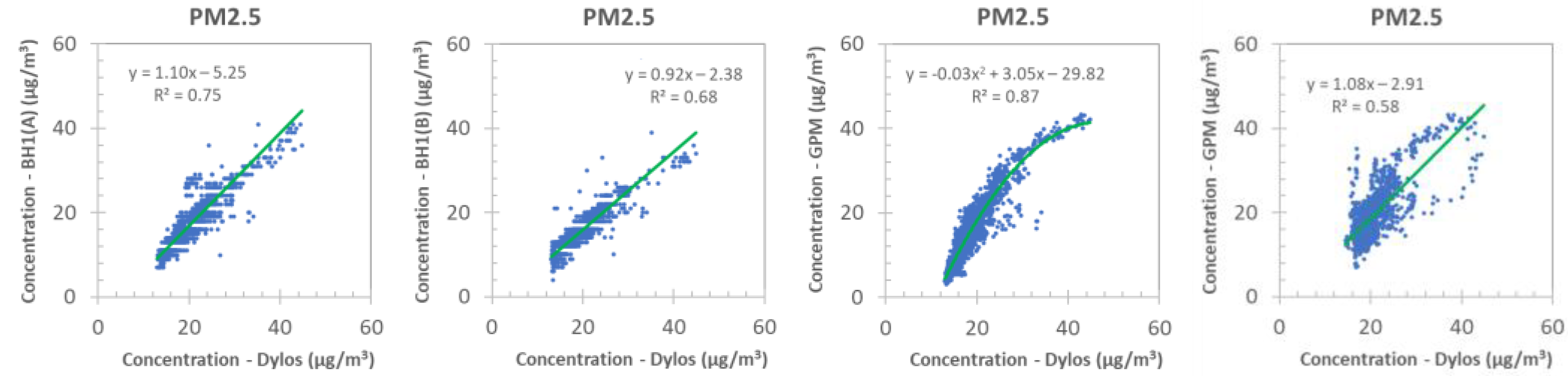
Besides the above devices, a research-grade Dylos DC-1700 (Dylos Corporation, Riverside, CA, USA) AQ monitor was applied to check and compare the performance of the LCSs and temporal trends of fine and coarse PNC. This monitor applies the same measurement principle as the studied LCSs. The sampling/measurement rate with this instrument was set to be continuous, which corresponded to one–one fine and coarse particle count data per minute. The PNC data were converted to PM concentrations using a second-order polynomial approach as recommended by Semple et al. [26]. Some of the monitoring results observed with the LCSs were also compared to those observed at a nearby AQ/meteorological station at Gilice Square (Budapest) of the Hungarian Air Quality Network [27].

2.3. Data Evaluation and Statistical Methods

The raw data from the LCSs were exported and converted into Excel. After that, they were first assessed for readings/measurement values inconsistent with persisting microclimatic conditions or related to calibration/diagnostic purposes or resetting of the sensors’ software. These values were discarded from the datasets before further processing. The 1–5 min data for GPM were calculated by averaging the registered data collected with a 1–60 s sampling rate.
The resultant “cleaned” data series were compared and statistically evaluated using Pearson’s bivariate correlation analysis and linear fits to the measurement points, using the multivariate least square method. The correlation coefficient (R) of the linear fit and related probability (p) values were calculated at a 99% confidence level. The AQI data were calculated using the stepwise function and the statistics of PM2.5 concentrations. Some predictions are made for human health effects at each sampling site on the base of the AQI, following the recommendation of US EPA [28]. The analytical performance parameters of the LCSs (e.g., bias, limit of detection) were calculated as described elsewhere [20].

3. Results

3.1. Monitoring Data from LCSs of the Same Type

3.1.1. GPM Sensors

As a very first experiment of this study, the performance of each air quality sensor of the same type was compared and evaluated. For this purpose, two GPM sensors were run simultaneously, each with synchronized internal clocks at the urban sampling site, indoors. As can be seen from the results compiled in Table 1, the air concentration of PM1, PM2.5, and PM10 ranged from non-detectable (n.d.) up to 29, 45, and 60 µg/m3, respectively, with averages of 4.9, 6.9, and 7.8 µg/m3, which correspond to low aerosol pollutant levels. As seen, slightly lower values could be attained by the use of the other GPM sensor.
The observed PM2.5 concentration is equal to an AQI maximum of 124, with an average of 28 (median: 25). These values correspond to mostly clean air quality, though the AQI of 124 already falls into the category of “Unhealthy for sensitive groups”, as classified by the US EPA [28]. The Ta and RH fluctuated between 20.6 and 25 °C and 40–60%, respectively, with averages of 23 °C and 50.8%, respectively, corresponding to rather stable indoor microclimatic conditions.
Looking at the experienced bias between the two GPM sensors (see Table 2), the two LCSs sometimes showed highly differing values in terms of high bias for PM1, PM2.5, and PM10, ranging from 0 to 400%, but with an average of 21–24% (median: 20–21%). These mean values are acceptable for monitoring purposes. Moreover, they are similar to those reported for LCSs in the literature [15,17]. The reason for the sometimes-high bias lies in the experienced low levels of indoor air PM, which in turn resulted in higher uncertainty between the monitoring data of the two concurrently operated sensors due to measurements performed close to the limits of detection of these devices.
On the other hand, indoor air parameters such as Ta and RH showed less bias: 1.5% and 8.8% on average, due to their less fluctuations in the indoor air. Nevertheless, when looking at the correlation graphs of the two sensors (Figure 2), strong correlations can be found between the monitoring data for each PM species, and the indoor microclimate data as well. The R value of the linear fit ranged between 0.93 and 0.97. However, a broader spread for AQI values lower than ≈70 could be seen. A similar data pattern was experienced for low values of PM, but to a much lesser degree (Figure 2).
Here, it is important to note that when measuring PM1, PM2.5, and PM10 concentrations below 20 µg/m3, the linear fits to simultaneous readings of the two GPM monitors showed decreased R values of 0.89, 0.89, and 0.82, respectively (Figure 3). Accordingly, a similar, lower correlation was found for the AQI (0.89), whereas for microclimatic parameters such as Ta and RH, still very high correlation coefficients were observed, i.e., 0.98 or higher.

3.1.2. BH1 Sensors

Secondly, the performance of one–one BH1 sensor was compared through the outdoor air sampling and analysis conducted at the urban site. This experiment was performed like that reported above, i.e., LCSs were operated concurrently, and the recorded air quality data were compared. As seen in Table 3, the concentration of PM1, PM2.5, and PM10 observed with the BH1(A) sensor ranged from 5 to 92, 7 to 114, and 7 to 128 µg/m3, with averages of 10.9, 14.3, and 15.8 µg/m3, respectively, which corresponds to low pollutant levels. These ranges do not differ significantly from those observed by the other sensor, BH1(B), i.e., 3–88, 4–103, and 4–122 µg/m3 and the related average values of 10.8, 14.2, and 15.6 µg/m3, respectively.
The Ta and RH fluctuated at relatively broad ranges, i.e., 4.1–21 °C and 28–72%, respectively, with averages of 12.3 °C and 49%, respectively, reflecting changing climatic conditions in the spring. In this sampling, the AQI values fluctuated between wide limits of 8 and 181, with a mean value of 56, corresponding to “Moderate” air quality. However, it should be recognized that the maximum AQI value of 181 falls in the “Unhealthy” range of US EPA classification [28].
As it appears in Figure 4, the data series of the two BH1 sensors for PM1, PM2.5, and PM10 correlate strongly with R values of 0.93 or better. The intercepts of the linear fit of the equations for PM1, PM2.5, and PM10 were observed to be 1.87, 2.41, and 2.55 µg/m3, respectively, showing consistency in the readouts of the sensors. Similarly good correlations could be observed for the AQI datasets. The microclimatic parameters of Ta and RH demonstrated even better correlation with R values higher than 0.98.

3.2. Monitoring Results for LCSs of Different Types

As the next stage of the study, the performance of different types of air quality LCSs was compared and evaluated indoors and outdoors. For this purpose, GPM and BH1 sensors were run simultaneously for about a week in indoor and outdoor environments.

3.2.1. Urban Site

According to the statistical data for indoor sampling compiled in Table 4, the monitoring results acquired by the application of BH1 are somewhat higher than those values acquired with the GPM sensor. The PM1, PM2.5, and PM10 concentrations observed with BH1 ranged between 4 and 42, 6 and 51, and 6 and 61 µg/m3, respectively, whereas for the GPM sensor, the range was n.d.–30, 1–45, and 1–57 µg/m3, respectively. On the other hand, there are significant differences between the average values obtained with the BH1 and the GPM sensors for PM1, PM2.5, and PM10, e.g., 8.3, 10.8, 12.2 µg/m3, and 2.7, 4.2, 4.8 µg/m3, respectively. These data still correspond to good air quality for this indoor environment. It can also be seen that the microclimatic conditions change modestly, e.g., Ta ranged from 23 to 26 °C with an average value of 24 °C, while RH fluctuated between 39 and 62% with an average of 48%.
When scrutinizing the correlation graphs of the PM data recorded by the GPM and BH1 sensors (Figure 5), the correlation coefficients of the linear fits show that the two data series correlate rather well, with R values of 0.78, 0.81, and 0.78, respectively (p = 0 at 0.01 confidence level).
However, it can also be seen that there is a positive bias in favor of the data series recorded by the BH1 sensor. This is manifested in the intercept of each equation of the linear fit to PM1, PM2.5, and PM10 data, being 6.57, 9.37, 11.46 µg/m3, respectively. As can be seen on Figure 5, most of these indoor air data series have a low reading due to the low air pollution levels for this spring sampling campaign. Consequently, when neglecting the low monitor readings (e.g., <5 µg/m3) for both sensors and reiterating the comparison of the newly obtained data series, better correlations for PM1, PM2.5, and PM10 are experienced, i.e., with R values of 0.76, 0.79, and 0.8, respectively.
An overview of the statistical data for outdoor sampling at the urban site by means of BH1 and GPM sensors is presented in Table 5. As expected, based on the indoor air measurements, higher values were usually experienced for the BH1 sensor as compared to those observed with the GPM monitor. The air levels of PM1, PM2.5, and PM10 observed with BH1 ranged from non-detectable (n.d.) up to 48, 60, and 67 µg/m3, respectively, whereas the corresponding ranges recorded with the GPM were 1–23, 1–37, and 1–45 µg/m3, respectively. Interestingly, there were no significant differences seen between the average (and median) values of PM1, PM2.5, and PM10 acquired by BH1 and GPM, i.e., 6.6, 9.1, and 9.8 µg/m3 and 6.1, 8.4, and 9.0 µg/m3, respectively. These data correspond to rather good air quality, though the AQI of 153 already falls into the “Unhealthy” category, according to the US EPA’s classification [28]. In this campaign, the outdoor microclimatic parameters the Ta fluctuated rather smoothly, i.e., between 7 and 22 °C (average: 14.3 °C), whereas the RH varied between broad limits, i.e., from 34 to 99% (average: 60%).
By examining the correlation graphs of various PM species obtained by the GPM and BH1 monitors outdoors (Figure 6), the regression coefficients of the linear fits demonstrates that the data series correlate rather well with R values of about 0.79. On the other hand, again, as for indoor air sampling, a slight positive bias can be experienced in favor of the data series registered with the BH1 monitor. This is well demonstrated in the intercept of each equation of the linear fit to PM1, PM2.5, and PM10 data, being 0.80, 3.48, 2.81 µg/m3, respectively.
However, it should be noted that these intercepts are much lower than those experienced for indoor air sampling of the same campaign/site (cf. Figure 5). As it appears in Figure 6, the data series of two different monitors applied for the outdoor climatic conditions also showed good correlations, e.g., for Ta and RH with R values of 0.99 and 0.98, respectively. The bias between them is about 4.4 °C and 5.08%, respectively, which may be due to their distance and local microclimatic fluctuations. On the other hand, the AQI series obtained with the two types of monitors showed significant difference in terms of the intercept and slope, whose result stems from the difference obtained in readings for low PM2.5 levels, e.g., <10 µg/m3.

3.2.2. Background Site

The summary of the statistical data for indoor sampling at the background site by means of BH1 and GPM sensors is presented in Table 6. Interestingly, the concentration of PM1, PM2.5, and PM10 recorded with the BH1 sensor is similar to that of observed with the GPM, ranging from 5 to 33, 7 to 42, and 7 to 48 µg/m3, respectively, whereas the corresponding ranges, recorded with the GPM, are 3–26, 5–41, and 5–52 µg/m3, respectively. The average values for BH1 are a bit higher for PM1, i.e., 15.2 µg/m3, compared to GPM (13.5 µg/m3), whereas lower mean values are experienced for PM2.5 and PM10, i.e., 19.5 and 21.7 µg/m3, respectively, with the corresponding GPM data of 21.1 and 24.7 µg/m3, respectively. The calculated AQI index calculated from PM2.5 values ranged between 29 and 117, reflecting the good air quality of the office in general, though an AQI higher than 100 shows “Unhealthy for Sensitive Groups” according to US EPA recommendation [28]. According to the registered microclimatic data, the indoor air showed slight fluctuations in terms of temperature and humidity (Table 6).
The correlation of the data series, recorded by the BH1 and GPM sensors, was examined for the urban background site too. As seen in Figure 7, the R values of these fits is about 0.95 or better, demonstrating a strong correlation between the two datasets. The slopes of the linear fits for PM1, PM2.5, and PM10 are 0.94, 1.29, and 1.47, respectively. The intercept of the linear fit to the PM1 data series is found to be positive (0.17 µg/m3) in favor of the GPM sensor, showing slightly lower readings for BH1, being rather negligible. On the other hand, negative intercepts for PM2.5 (–2.43 µg/m3) and PM10 (–5.1 µg/m3) were attained, which demonstrated slightly increased bias. As also seen in Figure 7, the two types of monitors developed strong correlations in terms of microclimatic parameters, such as Ta and RH, and for AQI, with R values of 0.74, 0.82, and 0.95, respectively.

3.2.3. Suburban Site

The correlation between the data series of BH1 and GPM sensors was evaluated at the suburban site, as depicted in Figure 8. The R values of the linear fits to the same kind of PMx data points are between 0.89 and 0.92, demonstrating that these parameters are well correlated. However, a stepwise increase in the intercept of the linear fit for PM1, PM2.5, and PM10 was observed, i.e., 7.6, 11.0, and 17.7 µg/m3, respectively. The positive values show the bias in terms of higher readings for the GPM. The slope of the linear fits for PM1 was slightly low (0.58), while for PM2.5 and PM10, it was acceptable, 0.82 and 1.15, respectively, which demonstrates the similar, linear response of the two different sensors to ambient aerosol concentrations. Nevertheless, it should be noticed that this site was characterized by high ambient RH, in the range of 40–95% (average: 83%). Thus, it is supposed that the high RH influences the readings of the two types of sensors, which is a likely assumption based on the literature [19,20,21,22]. Consequently, this possible effect was studied in the present work too (see Section 3.3). For AQI data, a similarly strong correlation was observed as above (R = 0.92) with a slope of 0.83 and an intercept of 27.
As seen in Figure 8, the two kinds of monitors developed significant correlations for the microclimatic parameters of Ta and RH with R values of 0.91 and 0.96, respectively. The slopes of the fit equations are also good, 0.92 and 1.03, with aptly small intercepts of 1.99 and 6.4, respectively. It should be noted here that the Ta readouts of BH1 below 0 °C could not be properly converted into the datasets somehow. For replacing those values, the concurrent data from the co-located GPM sensor was applied, where it was necessary. These results suggest that both LCSs appear to be adequate to monitor local PM and microclimatic changes indoors and in the outdoor air.

3.3. Effects of Microclimatic Parameters on PM Readings

As a further step of the study, the effects of RH on the PMx readings of the LCSs were evaluated at the suburban site (Figure 9). This site has higher RH conditions due to the proximity of the forest. As seen, for the BH1 sensor, fairly low slopes of the linear fits were observed with values of 0.07, 0.08, and 0.1, but with high intercepts of 23.8, 29.8, and 33.0 for PM1, PM2.5, and PM10, respectively. Low correlation could be seen between the RH values and the concentrations of various PM species. For PM1, PM2.5, and PM10, the linear fits were observed with R values of about 0.1, showing a weak correlation. On the other hand, for the GPM sensor, the slopes of the linear fits to the measurement points showed an increasing trend from PM1 (0.11), PM2.5 (0.23), and PM10 (0.43), while the corresponding intercepts were 14.6, 20, and 26.1, respectively. Moreover, the correlation coefficients were slightly higher (0.20–0.28) than in the case of the BH1 sensor. This shows the slight influence of the air RH on the readings of the GPM sensor, especially over 85% RH, as seen in Figure 9. Nevertheless, for each type of studied LCS, a relative humidity over 85% should be taken into account when evaluating PMx levels. For these cases, the use of a reference monitor and field calibration is necessary. It should be noted that RHs over 95% can have more influence on the PM readings from the LCSs, a condition that was also reported in the literature [15]. On the other hand, this experimental condition was not assessed in the present study, since the persisting meteorologic conditions during the sampling campaigns did not make it possible.
Besides the effects of RH, the influence of Ta on PMx readings of the LCSs were evaluated (Figure 10). As seen, the slopes of the linear fits for BH1 monitor ranged from −0.41 to −0.61 µg/m3 °C, while for the GPM they ranged between −0.49 and −2.24 µg/m3 °C, showing higher PM readings for low temperature values, e.g., below 5 °C. On the other hand, the intercepts of the equations ranged between 25 and 69 µg/m3, with increasing values towards the coarser PM fractions. The monitoring data from BH1 show insignificant correlation with the Ta changes, which is manifested in the low R values of about 0.14 for each PM fraction. On the other hand, the PM data obtained from the GPM sensor developed very weak dependency on varying Ta, which can be seen in the R values gradually increasing from 0.2 to 0.33 with increasing PM size fractions. Interestingly, a reverse trend for the dependency of PMx on changing Ta was observed for the spring period (data not shown here) as compared to the winter campaign.

3.4. Calibration of the Sensors

For calibration purposes, the PM2.5 readings of the LCSs were plotted against those values observed with the assistance of Dylos reference monitor (Figure 11). As it appears, the calibration fit of each BH1 sensor is linear over the studied PM2.5 concentration range with calibration slopes of 0.92 and 1.1, respectively, and with low intercepts of −5.25 and −2.38, respectively. The correlation coefficients of these fits are also acceptable, with R values of 0.87 and 0.83, respectively, showing strong correlation between the dataset pairs. On the other hand, the PM2.5 data from the GPM monitor develop a rather second-order function, which is due to the deviation in the readings in the low concentration range, i.e., for values of lower than about 20 µg/m3. When excluding these data from the evaluation, it can be seen that the datasets can be approached well with a linear equation (slope: 1.08, intercept: −2.91). Overall, the GPM and BH1 sensors follow the PM2.5 readings of the reference monitor quite well. Consequently, these LCSs do not usually require calibrations against reference monitors, apart from the air pollution levels falling into the low PM range and when measuring ambient air under high RH conditions as noted above.

3.5. Temporal Trends of Indoor and Outdoor Air Quality

3.5.1. Urban Sampling Site

The time series for the spring campaign (24–30 May 2021) observed with one–one BH1 and GPM sensors at the urban site is depicted in Figure 12.
As seen, the air quality follows the daily trend of air pollution during the weekdays: peak hours encountered in the mornings (e.g., from 6 a.m. to 9 a.m.) and the evenings (from 4 p.m. to 8 p.m.), whereas at the weekend, only Saturday morning and Sunday evening have somewhat higher peaks for each three PM species. Some high night PM readings are also experienced in this period. Though the daytime emissions are mostly ruled by those originating from the passing of local motor vehicular traffic, it is also possible that biomass burning, in the form of barbecues, occurred during the campaign, and a contributing factor, especially at the weekend.
The indoor data series of the same campaign is depicted in Figure 13. As seen, the local outdoor air contributes to the indoor trends, exemplified in the appearance of higher readings for the monitored PM species during the peak traffic hours as above. On the other hand, some midday peaks can be seen, reaching values as high as 54–65 µg/m3. These sharp increases in the indoor PM levels are due to related cooking activities in the kitchen and the proximity of the kitchen to the sampling spot (anteroom), and likely ingress of particles into the latter.
It could also be seen that the GPM sensor gave rather sharper peaks of aerosol concentration changes than BH1, likely due to the higher resolution of the former (1 min), thus resulting in more accurate average PM values for local air quality.
The outdoor air quality was also assessed for a winter campaign week (6–12 December 2021), as depicted in Figure 14. As can be seen, the daily concentration of PM1, PM2.5, and PM10 fluctuated between 10 and 69, 15 and 113, and 17 and 138 µg/m3, with averages of 27, 44, and 54 µg/m3, respectively. These PM2.5 data correspond to an AQI range of 58–181, with an average of 119, which is already a high value, classified as “Unhealthy for sensitive groups” according to the US EPA [28]. The temporal PM trend suggests the periodic influence of local traffic on the local air quality, manifested in the periodically enhanced PM concentration during the morning and the afternoon rush hours. Moreover, the effects of wood-fueled heating could be observed too, which caused increased background aerosol levels and a few peaks for each PM species, mostly experienced during the evening and the night hours. Overall, these data exhibit far higher PM levels than those obtained for the same sampling site in the spring campaign (cf. Figure 12).

3.5.2. Background Site

The temporal trends observed during the winter campaign (6–12 December 2021), with the application of the GPM sensor at the background site, outdoors, is depicted in Figure 15. As seen, elevated levels of PM1, PM2.5, and PM10 were experienced, reaching as high values as 30, 50, and 75 µg/m3, respectively. The enhanced PM background can be seen on weekdays, while on weekends, lower aerosol concentrations were obtained. Therefore, it is supposed that the emissions of the local heating station of the campus is a main source of this enhanced background PM levels. Moreover, during winter, several people living in residential houses of the nearby settlements apply wood-/coal-fueled heating for their homes. This type of anthropogenic emission can deteriorate the air quality at the concerned sampling site for each three PM fractions by enhancing the local background PM levels. Fairly high RH values of about 80–92% were observed at this sampling site with air temperatures as low as close to freezing. The AQI values for outdoor air of this site ranged between 28 and 152 (average: 97, median: 100).
The indoor data recorded for the same sampling campaign are depicted in Figure 16. As can be seen, the pattern of fluctuation in the concentration of various PM species is similar to those observed for outdoor air. During this indoor sampling, the GPM sensor detected peaks of PM1, PM2.5, and PM10 as high as 26, 40, and 50 µg/m3, respectively. The increase in PM2.5 levels and the related AQI values point towards being “Unhealthy for sensitive groups”, which is a concern for a group of people attending the campus and related offices.

3.5.3. Suburban Site

The temporal evolution of PM species and the microclimatic parameters observed during the winter campaign (6–12 December 2021) with the application of the GPM sensor at the suburban site, outdoors, are depicted in Figure 17. As shown, the concentrations of PM1, PM2.5, and PM10 fluctuated and showed peak values of 55, 107, and 190 µg/m3, respectively.
This site also showed the influence of nearby motor vehicular traffic, on a main road, and as a result, enhanced background PM levels. Rush hours were characterized by somewhat increased levels of air pollution, though the local background PM level was generally high. An increase in PM concentrations was also observed during evening and night hours, when the local residential houses were heated, most likely with wood/coal combustion, manifested also in the large increase in coarse PM fractions. According to the detected PM2.5 levels, the AQI of this site was also assessed, the value of which ranged between 55 and 178 with an average of 113. These values are relatively high, corresponding to the air quality class “Unhealthy for sensitive groups”. On some sampling days, the AQI falls into the “Unhealthy” category, according to the US EPA classification [28]. This demonstrates similar air quality for the investigated suburban site, as compared to the urban and the background sites. This is most likely due to the combined effects of the nearby emissions of the motor vehicular traffic and wood/coal fueled heating in the residential houses.

3.6. Analytical Performance of the Sensors

The analytical performance of the LCSs was assessed through the examination of several air quality readings and observations for suspended PM, such as the lowest and highest readouts in indoor air campaigns, for instance, when the pollution load could be much higher than that of the outdoor, due to poor ventilation of the house and cooking activities during sampling. On the basis of these data, for the GPM and BH1 sensors, a maximum of 256 and 450 µg/m3 was found as the highest ultimate PM values, respectively. As regards the sensitivity of the two types of sensors, GPM possesses higher sensitivity (limit of detection: 2 µg/m3) than BH1 (limit of detection: 7 µg/m3), manifested also in changes in the readouts for lower PM concentrations. The GPM sensor, exhibiting as high a temporal resolution as 1 s, is more sensitive for slight changes in air quality than the BH1 monitor, which possesses only 1–5 min as the highest resolution.
The observed PM readings by the LCSs were also tested against the Dylos air quality monitor, for instance, in the winter campaign. The readout pattern for the particle count of fine and coarse suspended particulate matter is found to be very similar to those observed with the LCSs as above, specifically for PM2.5 and PM10 (see Figure 16a vs. Figure 16b). To assess the accuracy of the monitoring data by LCSs, the PM concentrations recorded in spring were assessed from hourly average series of a nearby official air quality station, located at Gilice Square, Budapest (Table 7). As seen, the average/median values approach fairly well those data observed at the urban sampling site with the assistance of BH1 monitors for the same sampling period (Table 3).

4. Conclusions

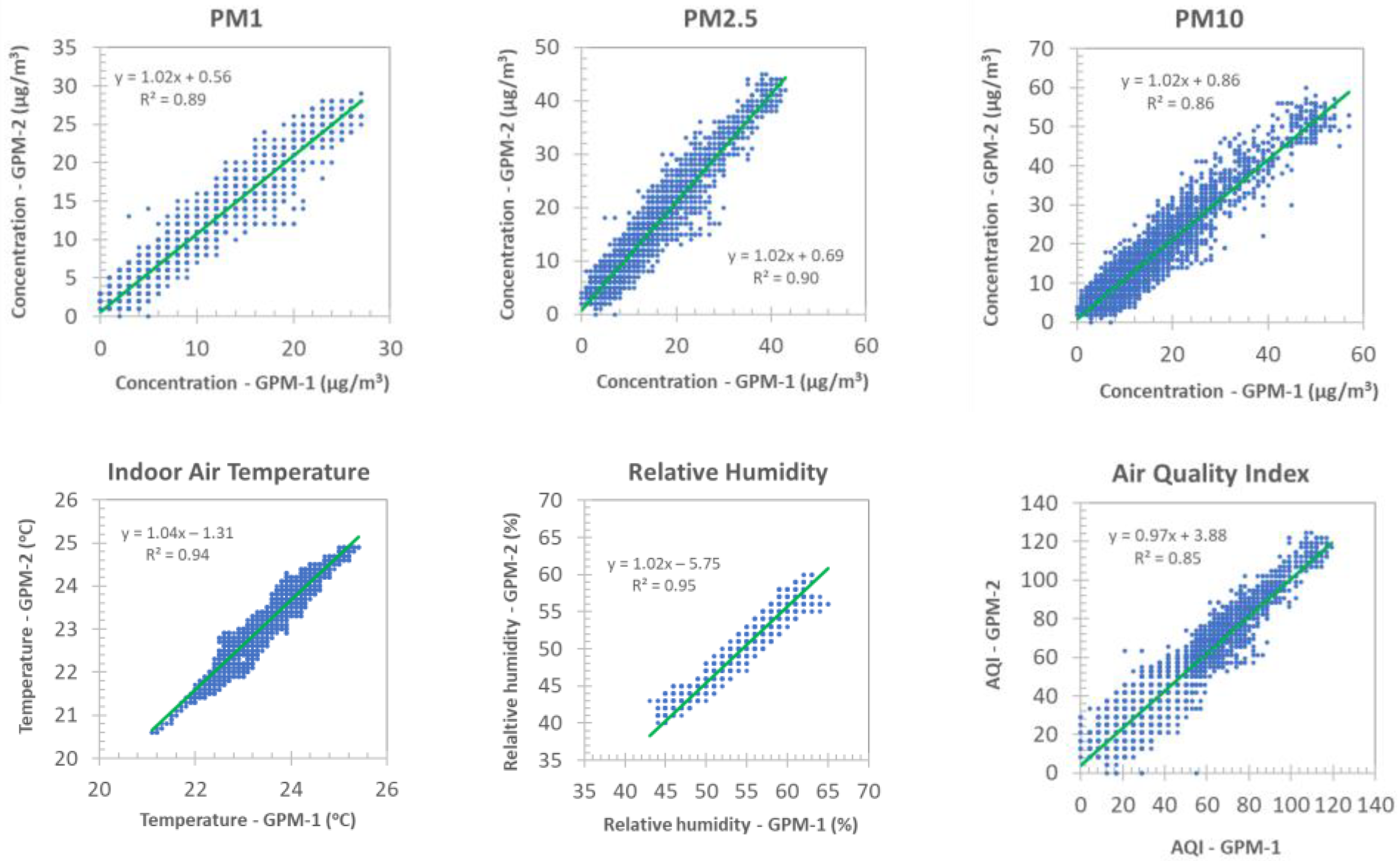
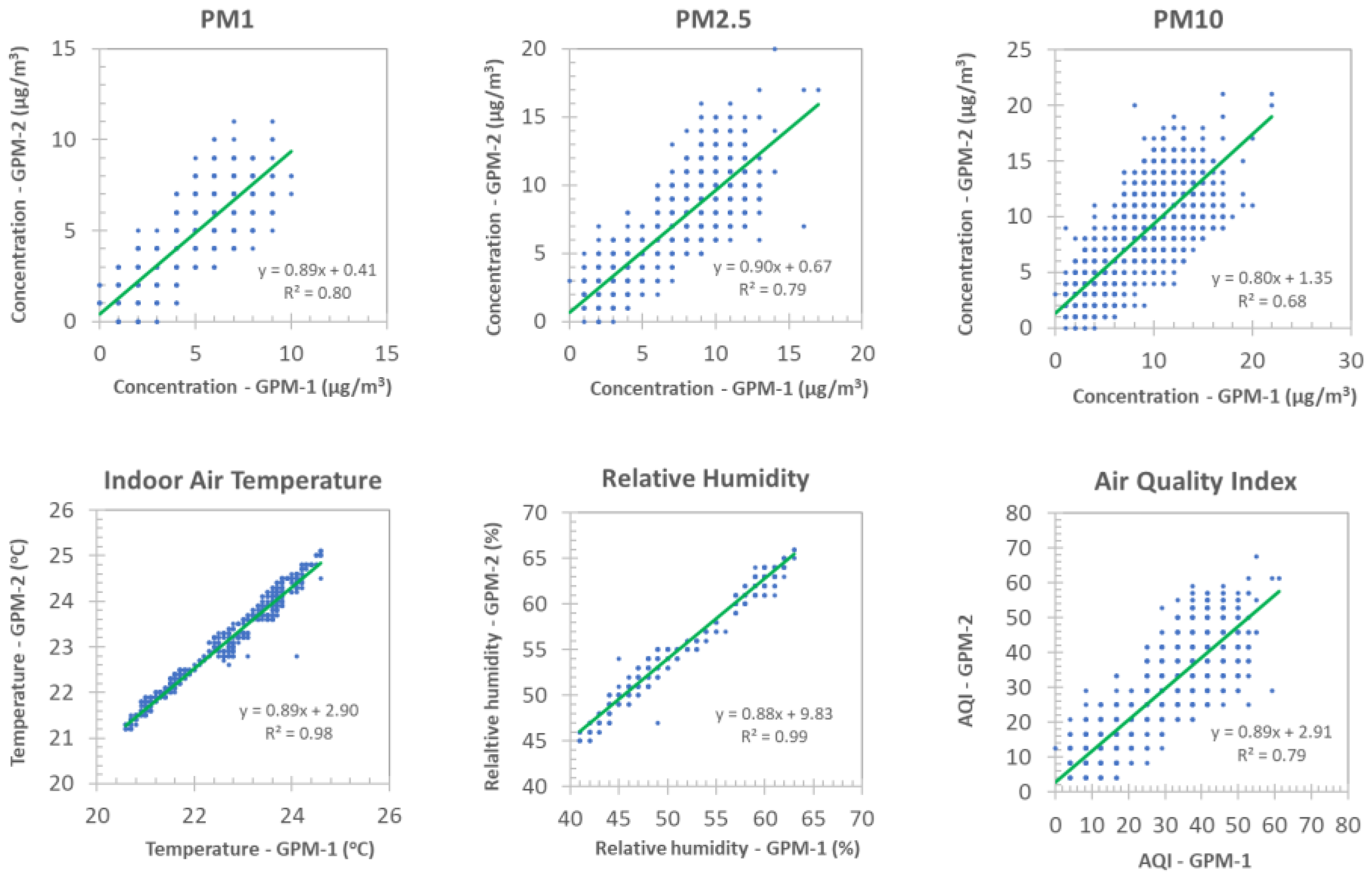
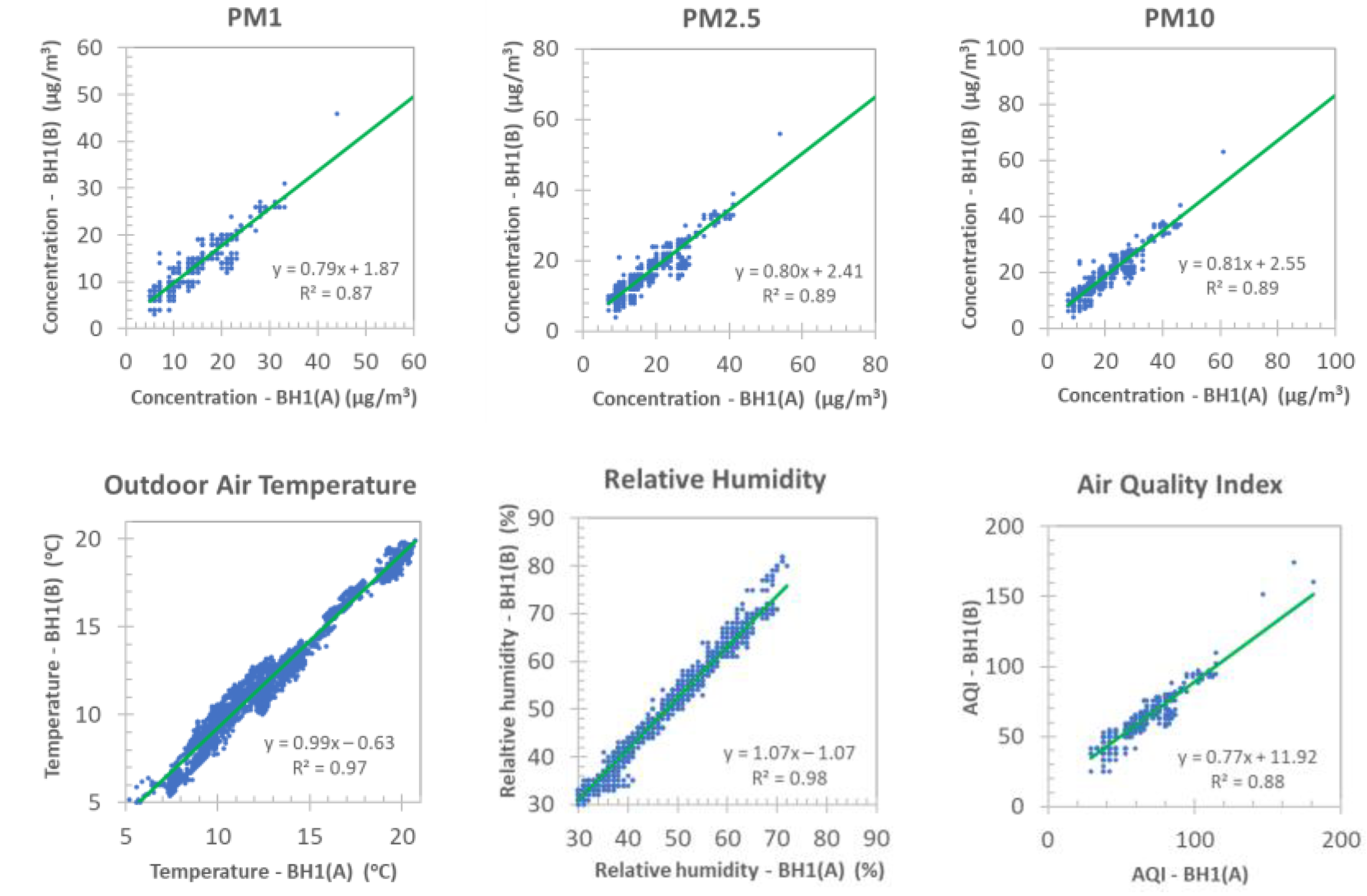
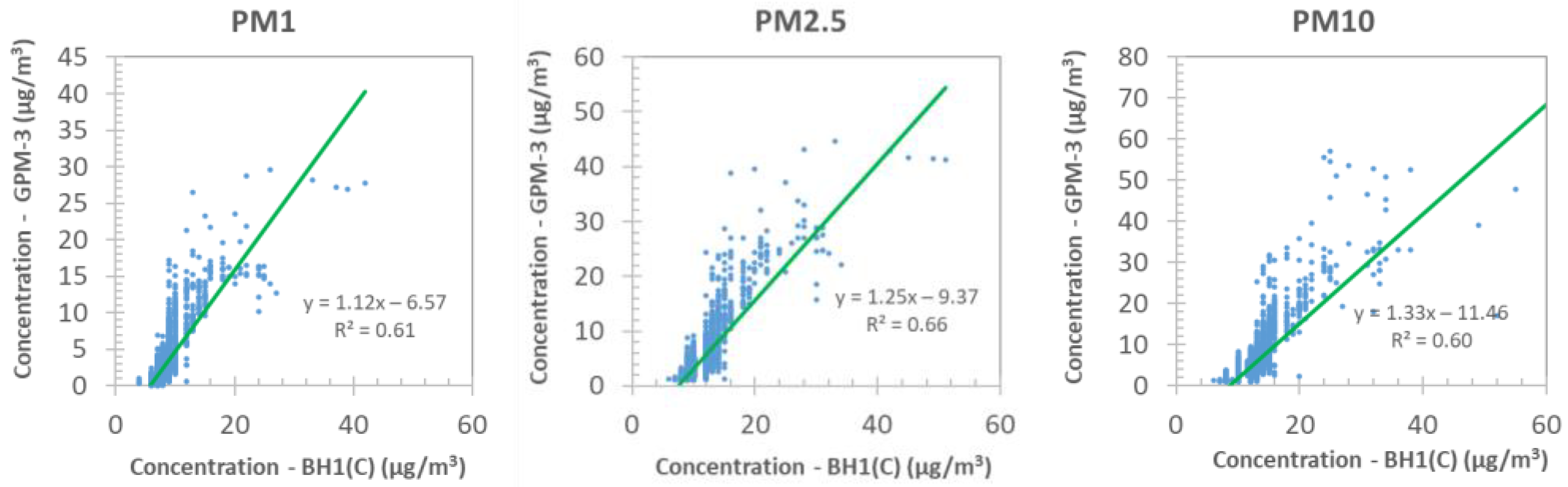
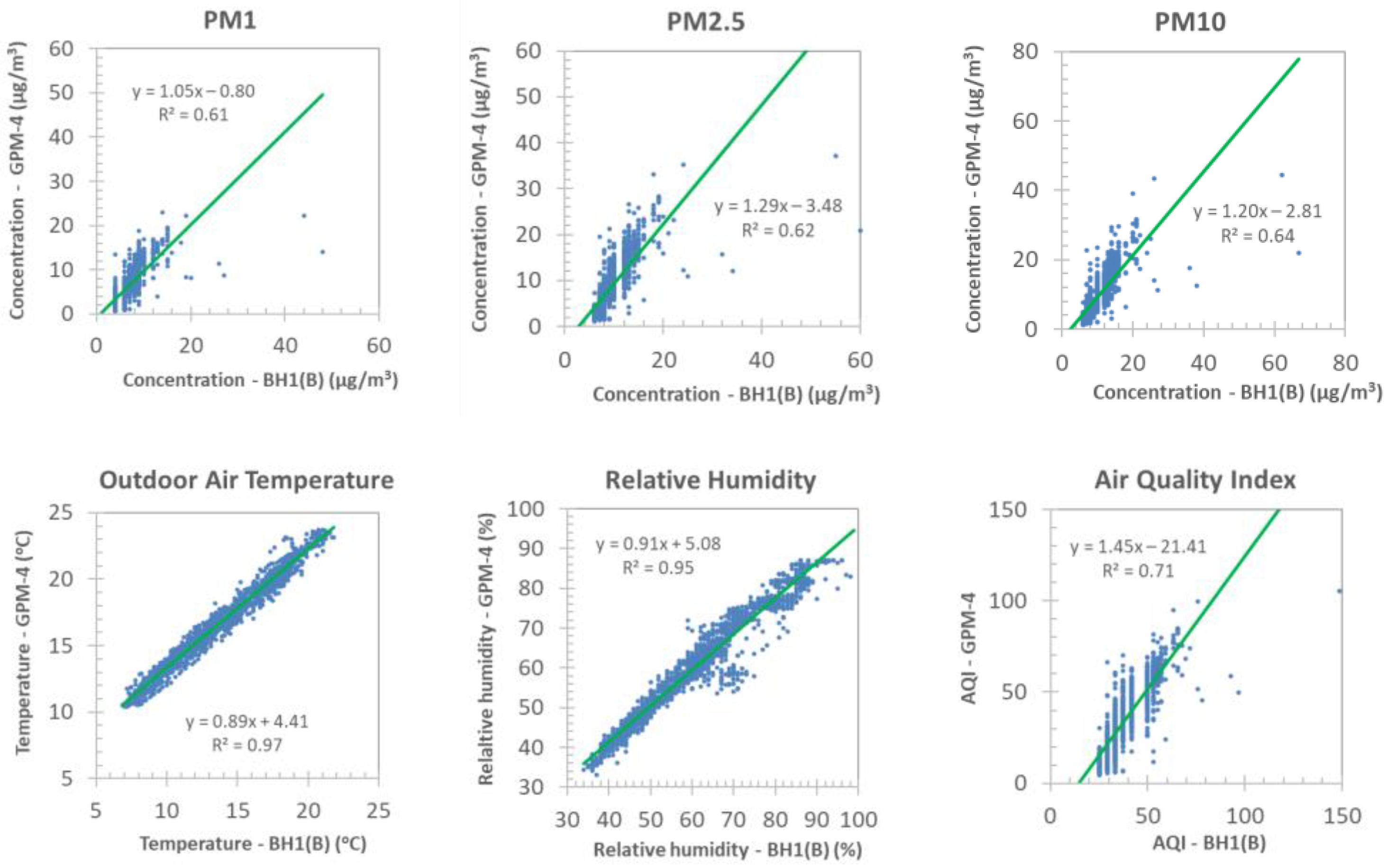
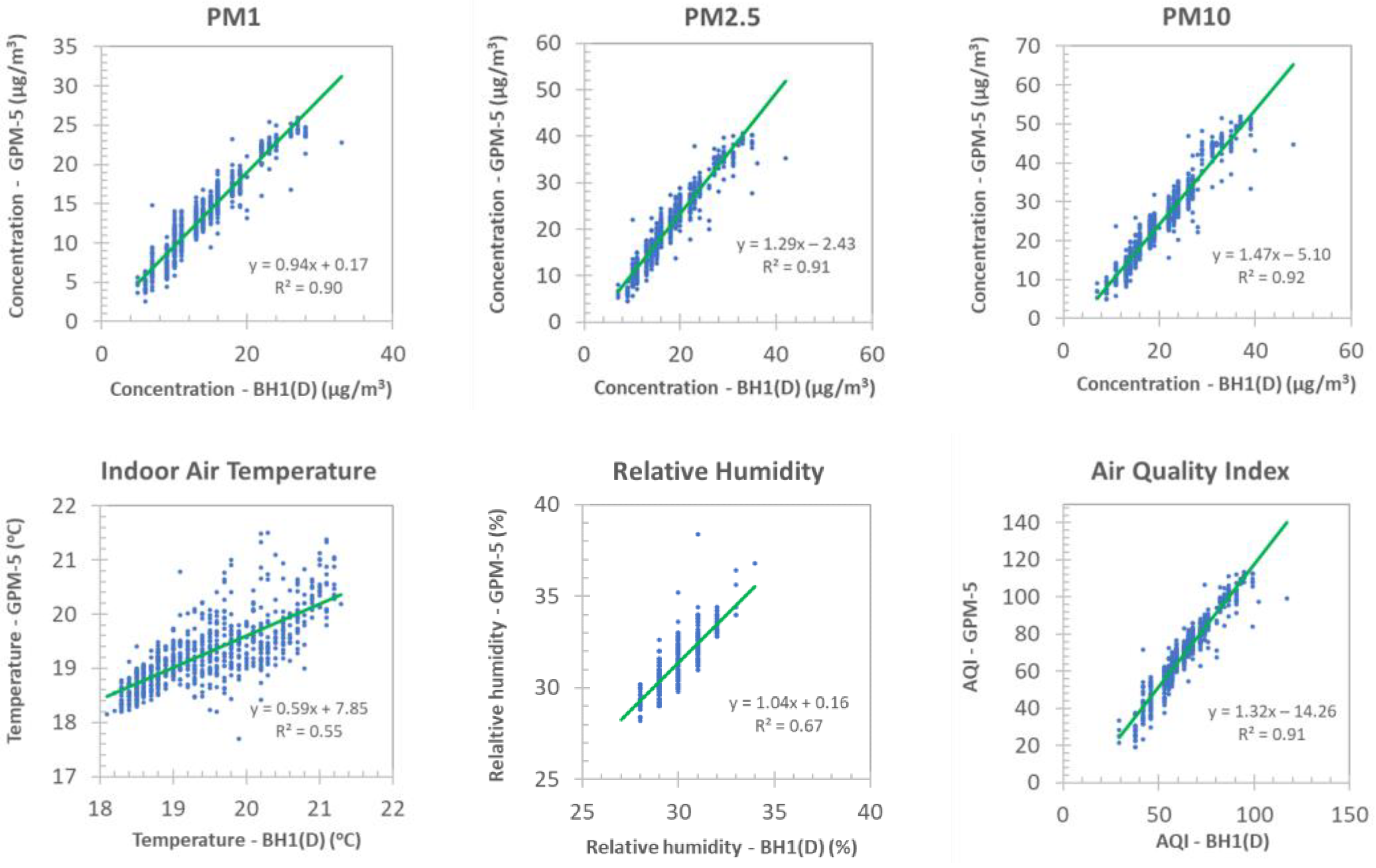
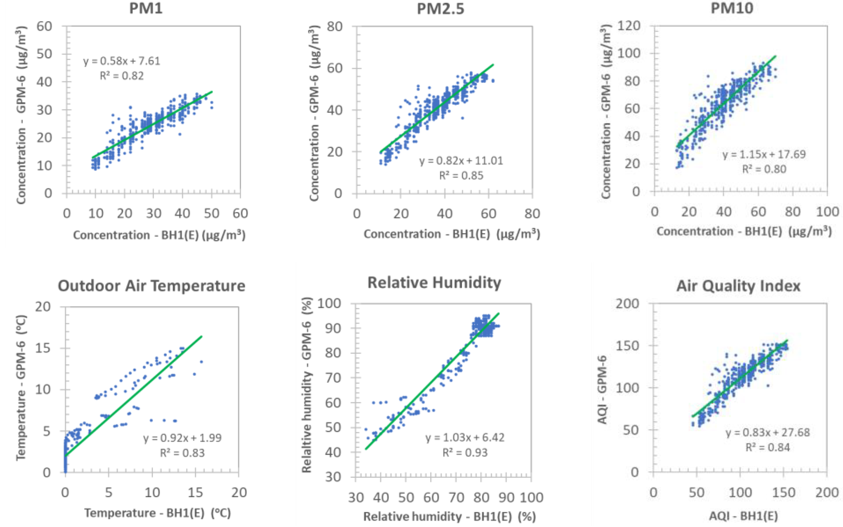
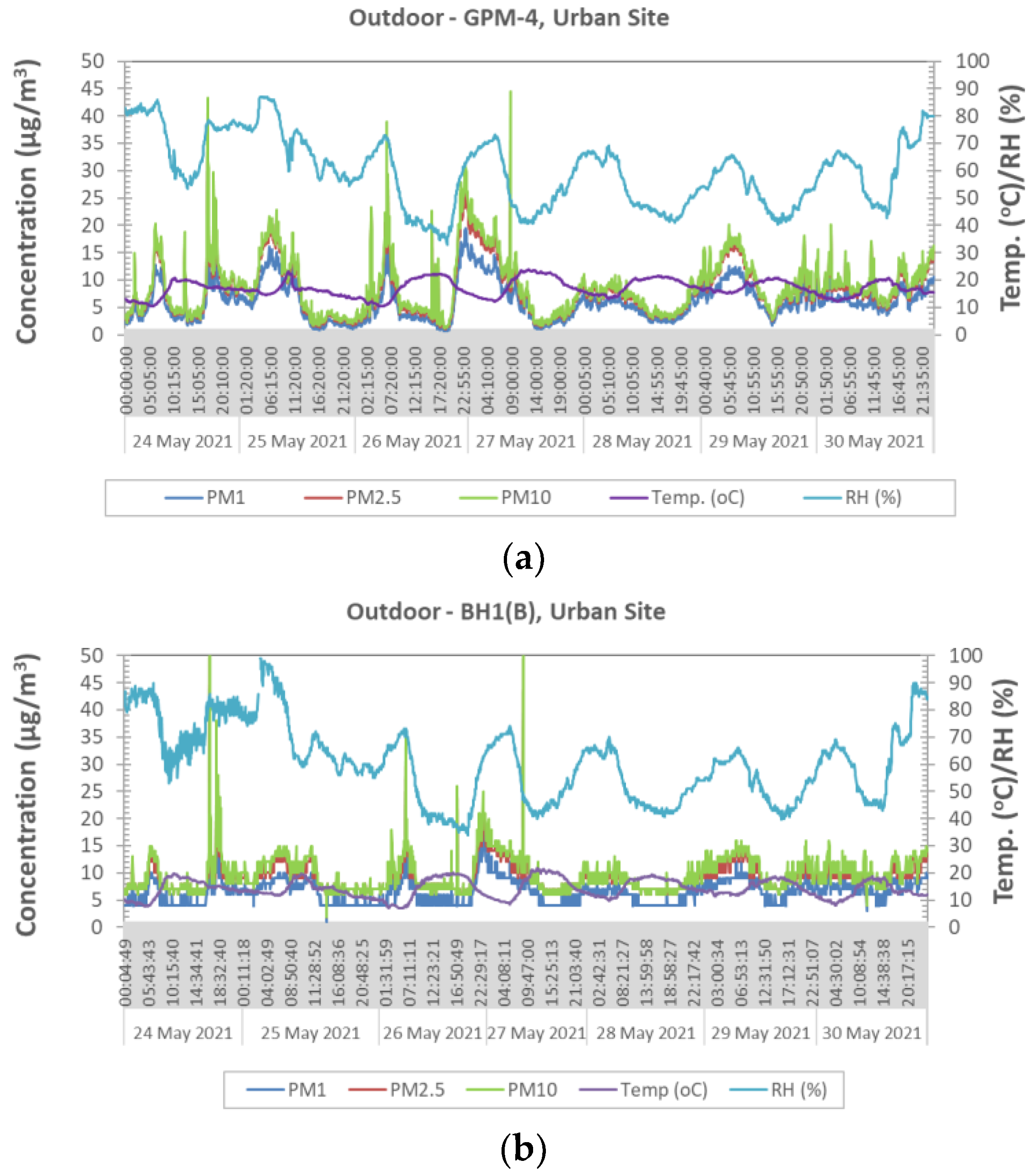
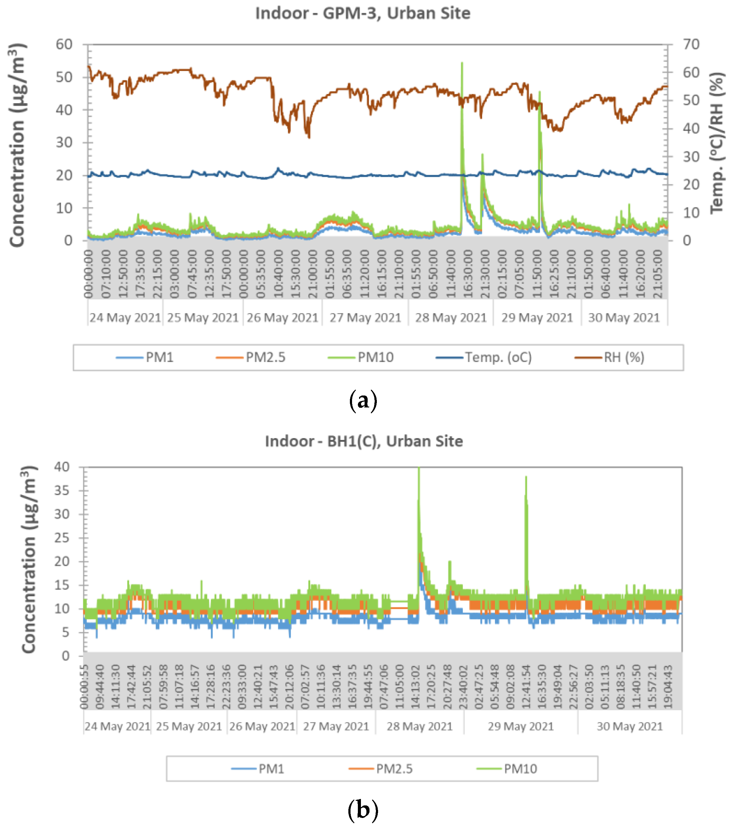
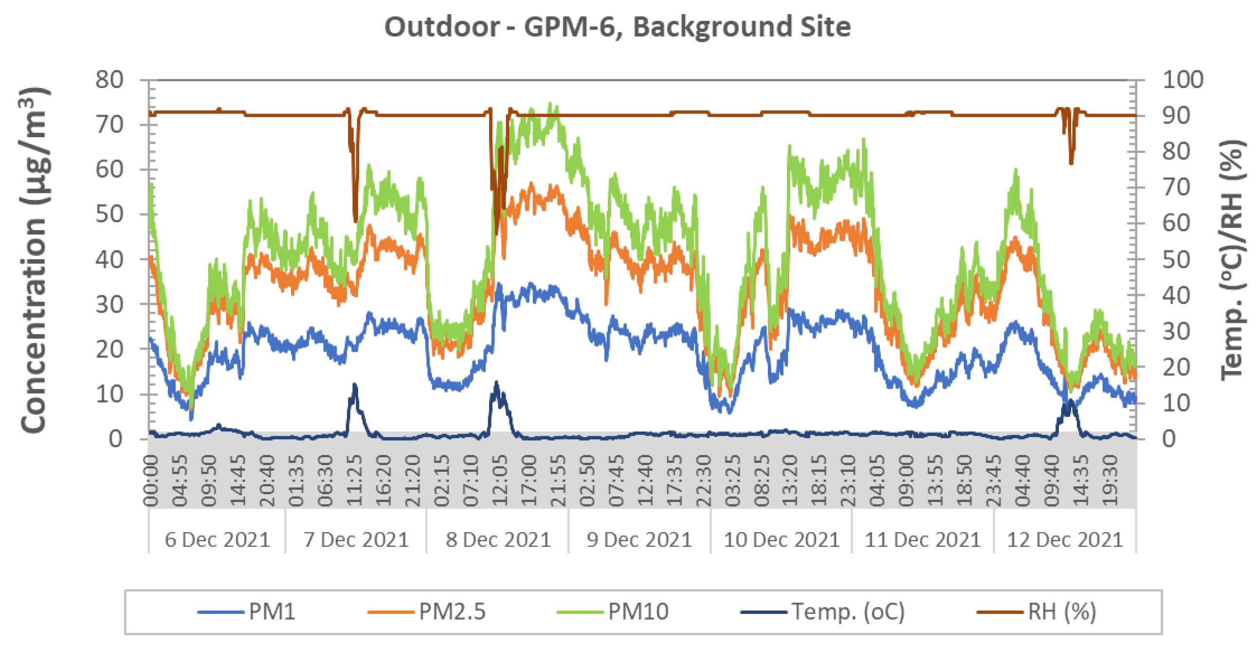
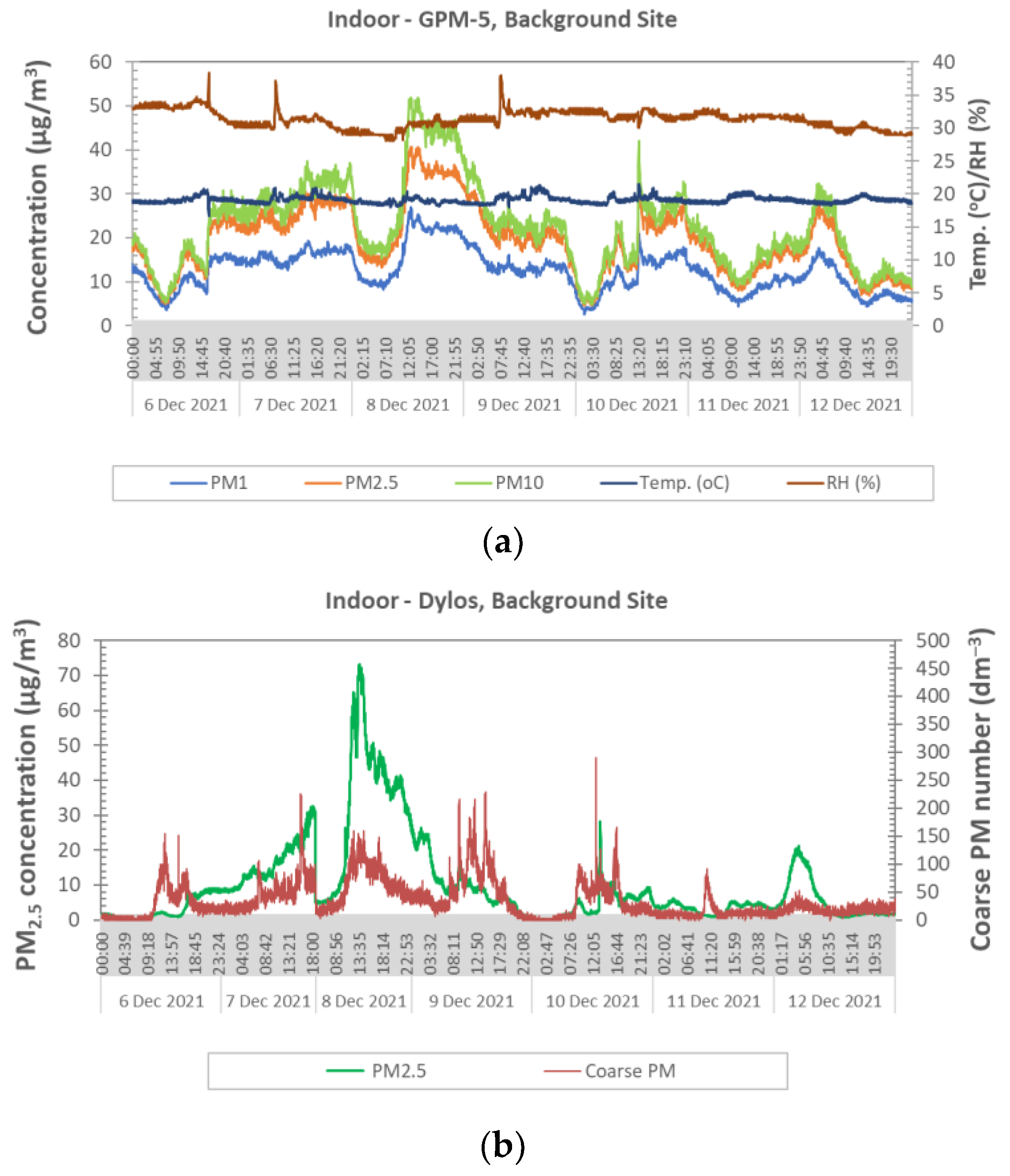
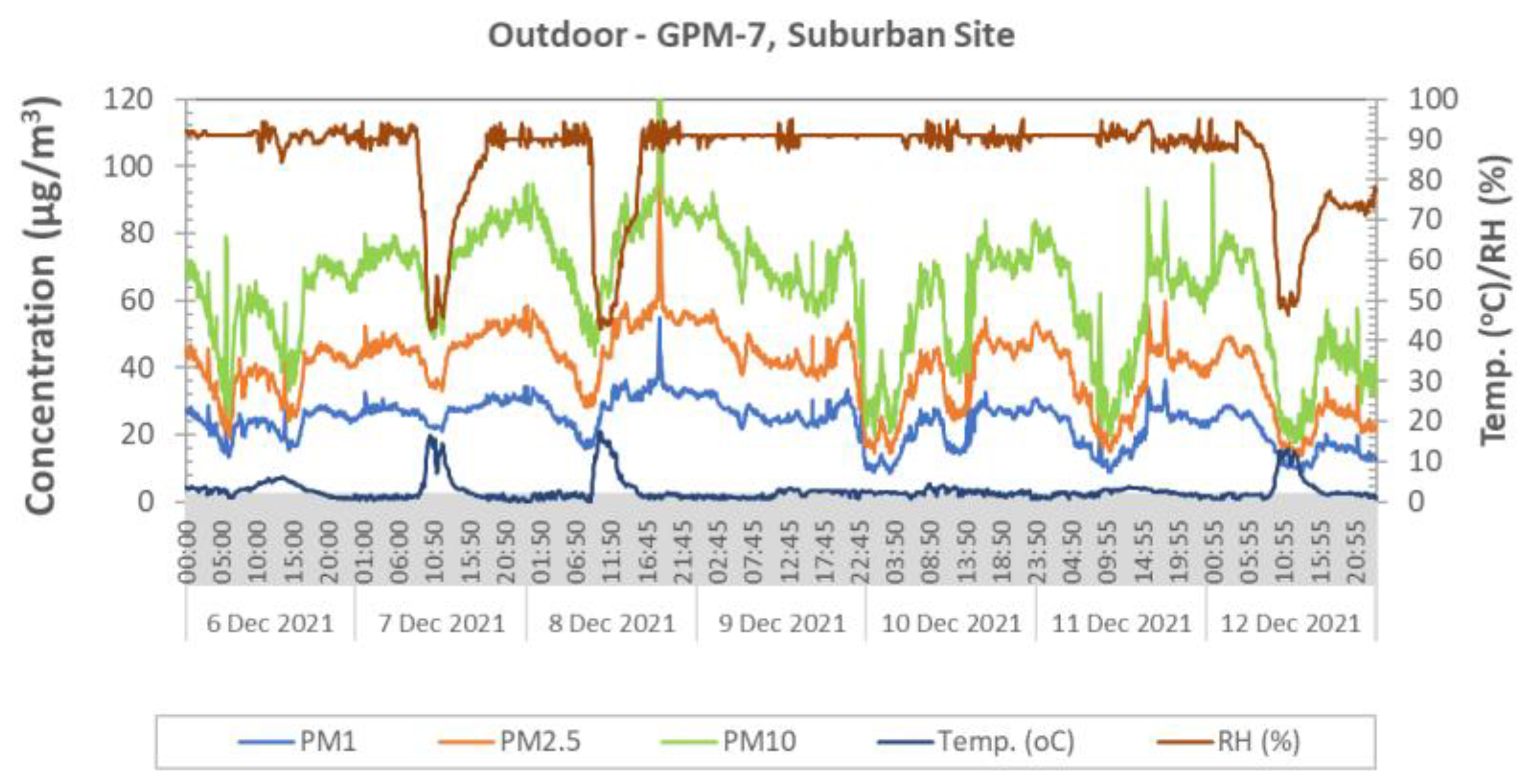
In the present study, two types of LCSs (Geekcreit PMx and Bohu BH1) were tested and evaluated for indoor and outdoor sampling of air suspended PM, performed at three sites of different anthropogenic influence in Budapest, Hungary. In general, both LCSs were found to be well applicable to indoor and outdoor monitoring. It could also be experienced that the GPM sensor gave rather sharper peaks of aerosol concentration changes than BH1 due to the higher temporal resolution applicable with this type of device (e.g., down to 1 s). Moreover, this monitor gave lower PM values in some instances, at the urban and suburban sampling sites as compared to those observed with the BH1 sensor. This is most likely due to a more sensitive detection assembly though lower aerosol load, and thus a lower upper limit of the aerosol concentration detectable by the use of this device. A definite drawback of the GPM sensor is the mandatory use of a control PC with software for data collection and storage, which limits the field applications. On the other hand, the BH1 sensor has its own built-in battery, data storage, and control software, which features provide it with the facility of self-standing operation for several hours, depending on the adjusted sampling rate.
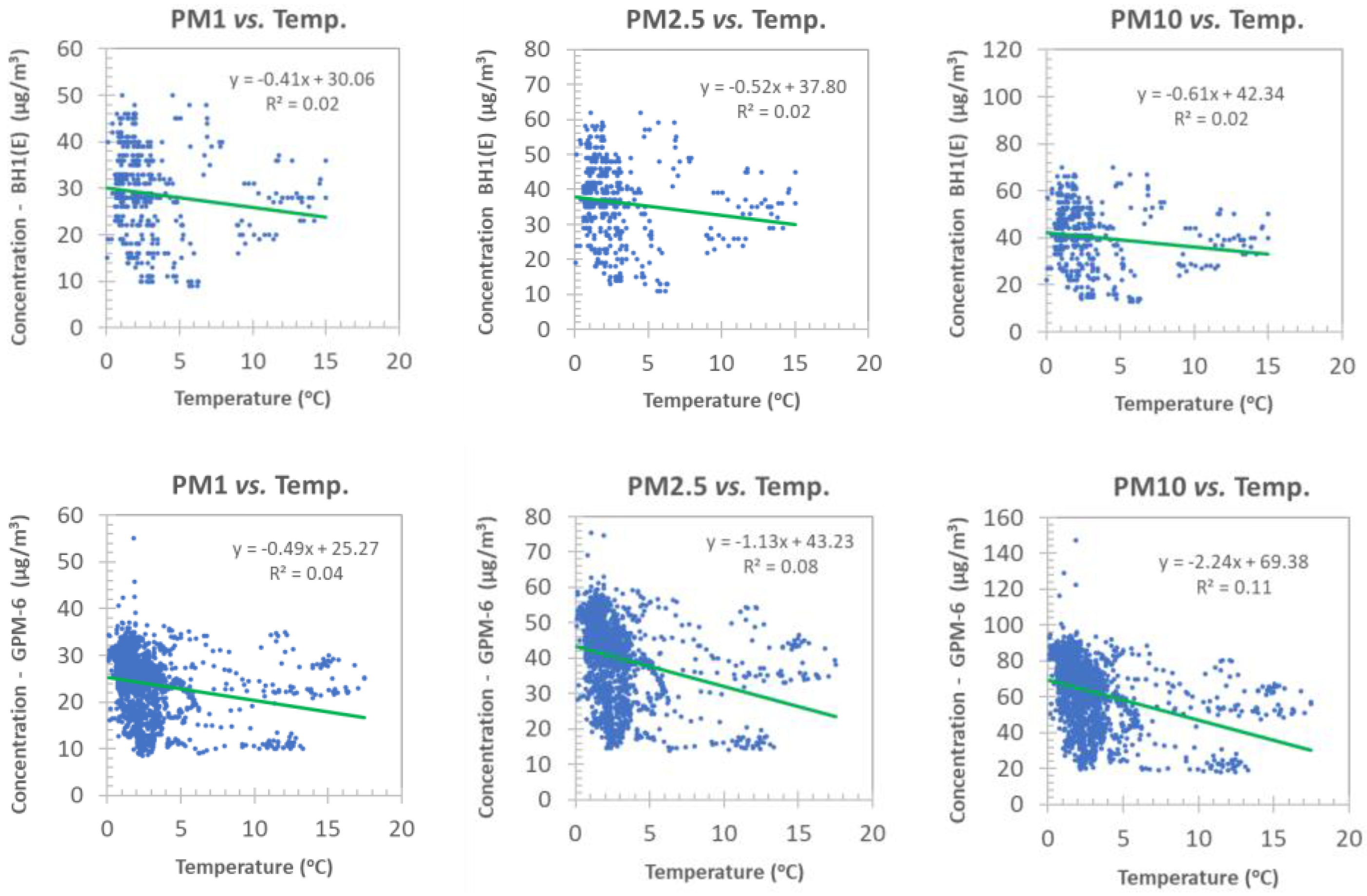
The analytical performances of the studied LCSs were found to be similar, though the BH1 had in general somewhat higher readings for PM levels lower than 10–15 µg/m3, especially outdoors at the urban site, where the emissions from the local motor vehicular traffic prevailed as an air pollution source during the campaigns. Nevertheless, the bias found between the two types of sensors is negligibly low at higher readings, the concentration range of aerosols being important from a human health point of view. The relative humidity had some influence on PMx readings for both sensors, from which the GPM sensor was more sensitive to changes in this microclimatic parameter. A relative humidity higher than 85% had an additive effect on the PMx values. On the other hand, the ambient air temperature had negligible/low effects on PM data. Recalibration of the LCSs at each specific site against a reference AQ monitor is recommended to attain more accurate PM readings.
The studied LCSs have also been found to be well applicable for tracking the impact of local traffic, the related peak hours, and to reveal the cooking and wood-fueled heating activities nearby. For the three study sites, rather low health impacts of atmospheric suspended matter can be expected on the basis of the present study. However, indoor air quality could be seen as deteriorating quickly, for instance, due to local heating and cooking activities, though its background level was also found to be highly dependent on the outdoor air quality.
Summarizing the above acquired results, they suggest that both types of air quality sensors are adequate to monitor local PM and microclimatic changes indoors and in the outdoor air, towards supporting the measurements of official air quality stations as well as using their data series as input parameters for atmospheric dispersion models.

Author Contributions

Conceptualization, L.B., B.P., A.G.M. and N.S.; methodology, L.B., B.P., A.G.M. and N.S.; validation, L.B.; investigation, L.B., A.G.M. and N.S.; resources, L.B. and N.S.; data curation, L.B. and N.S.; writing—original draft preparation, L.B.; writing—review and editing, L.B., B.P., A.G.M. and N.S.; visualization, L.B.; supervision, L.B.; project administration, L.B.; funding acquisition, L.B. All authors have read and agreed to the published version of the manuscript.

Funding

This research received no external funding. One of the authors (L.B.) gratefully thanks the internal funding supplied for the chemical spectroscopic laboratory in the Wigner Research Centre for Physics.

Institutional Review Board Statement

Not applicable.

Informed Consent Statement

Not applicable.

Data Availability Statement

The data presented in this study are available on request from the corresponding author. The data are not publicly available due to file size limitations. A part of the data available in a publicly accessible repository that does not issue DOIs. This data can be found here: http://www.levegominoseg.hu/automata-merohalozat (access on 18 June 2022).

Conflicts of Interest

The authors declare no conflict of interest.

References

  1. Dockery, D.W.; Speizer, F.E.; Stram, D.O.; Ware, J.H.; Spengler, J.D.; Ferris, B.G., Jr. Effects of inhalable particles on respiratory health of children. Am. Rev. Respir. Dis. 1989, 139, 587–594. [Google Scholar] [CrossRef] [PubMed]
  2. IPCC. Climate Change 2021: The Physical Science Basis, Sixth Assessment Report; Cambridge University Press: Cambridge, UK, 2021. [Google Scholar]
  3. Anaf, W.; Bencs, L.; Van Grieken, R.; De Wael, K.; Janssens, K. Indoor particulate matter in four Belgian heritage sites: Case studies on the deposition of dark-colored and hygroscopic particles. Sci. Total Environ. 2015, 506–507, 361–368. [Google Scholar] [CrossRef] [PubMed]
  4. Leung, D.Y.C. Outdoor-indoor air pollution in urban environment: Challenges and opportunity. Front. Environ. Sci. 2015, 2, 69. [Google Scholar] [CrossRef]
  5. Deutsch, F.; Vankerkom, J.; Janssen, L.; Janssen, S.; Bencs, L.; Van Grieken, R.; Fierens, F.; Dumont, G.; Mensink, C. Modelling concentrations of airborne primary and secondary PM10 and PM2.5 with the BelEUROS-model in Belgium. Ecol. Modell. 2008, 217, 230–239. [Google Scholar] [CrossRef]
  6. Moltchanov, S.; Levy, I.; Etzion, Y.; Lerner, U.; Broday, D.M.; Fishbain, B. On the feasibility of measuring urban air pollution by wireless distributed sensor networks. Sci. Total Environ. 2015, 502, 537–547. [Google Scholar] [CrossRef] [PubMed]
  7. Jerrett, M.; Donaire-Gonzalez, D.; Popoola, O.; Jones, R.; Cohen, R.C.; Almanza, E.; de Nazelle, A.; Mead, I.; Carrasco-Turigas, G.; Cole-Hunter, T.; et al. Validating novel air pollution sensors to improve exposure estimates for epidemiological analyses and citizen science. Environ. Res. 2017, 158, 286–294. [Google Scholar] [CrossRef] [PubMed]
  8. Mead, M.I.; Popoola, O.A.M.; Stewart, G.B.; Landshoff, P.; Calleja, M.; Hayes, M.; Baldovi, J.J.; McLeod, M.W.; Hodgson, T.F.; Dicks, J.; et al. The use of electrochemical sensors for monitoring urban air quality in low-cost, high-density networks. Atmos. Environ. 2013, 70, 186–203. [Google Scholar] [CrossRef] [Green Version]
  9. Castell, N.; Dauge, F.R.; Schneider, P.; Vogt, M.; Lerner, U.; Fishbain, B.; Broday, D.; Bartonova, A. Can commercial low-cost sensor platforms contribute to air quality monitoring and exposure estimates? Environ. Int. 2017, 99, 293–302. [Google Scholar] [CrossRef]
  10. Thorpe, A.; Walsh, P.T. Comparison of Portable, Real-Time Dust Monitors Sampling Actively, with Size-Selective Adaptors, and Passively. Ann. Occup. Hyg. 2007, 51, 679–691. [Google Scholar]
  11. Salimifard, P.; Rim, D.; Freihaut, J.D. Evaluation of low-cost optical particle counters of monitoring individual indoor aerosol sources. Aerosol Sci. Technol. 2020, 54, 217–231. [Google Scholar] [CrossRef]
  12. Hagan, D.H.; Gani, S.; Bhandari, S.; Patel, K.; Habib, G.; Apte, J.S.; Hildebrandt Ruiz, L.; Kroll, J.H. Inferring aerosol sources from low-cost air quality sensor measurements: A case study in Delhi, India. Environ. Sci. Technol. Lett. 2019, 6, 467–472. [Google Scholar] [CrossRef] [Green Version]
  13. Oluwadairo, T.; Whitehead, L.; Symanski, E.; Bauer, C.; Carson, A. Effects of Road Traffic on the Accuracy and Bias of Low-Cost Particulate Matter Sensor Measurements in Houston, Texas. Environ. Res. Public Health 2022, 19, 1086. [Google Scholar] [CrossRef]
  14. Wahlborg, D.; Björling, M.; Mattsson, M. Evaluation of field calibration methods and performance of AQMesh, a low-cost air quality monitor. Environ. Monit. Assess. 2021, 193, 251. [Google Scholar] [CrossRef]
  15. Crilley, L.R.; Shaw, M.; Pound, R.; Kramer, L.J.; Price, R.; Young, S.; Lewis, A.C.; Pope, F.D. Evaluation of a low-cost optical particle counter (Alphasense OPC-N2) for ambient air monitoring. Atmos. Meas. Tech. 2018, 11, 709–720. [Google Scholar] [CrossRef] [Green Version]
  16. Yuval; Molho, H.M.; Zivan, O.; Broday, D.M.; Raz, R. Application of a sensor network of low cost optical particle counters for assessing the impact of quarry emissions on its vicinity. Atmos. Environ. 2019, 211, 29–37. [Google Scholar]
  17. Markowich, K.M.; Chiliński, M.T. Evaluation of two low-cost optical particle counters for the measurement of ambient aerosol scattering coefficient and Ångström exponent. Sensors 2020, 20, 2617. [Google Scholar] [CrossRef]
  18. Sousan, S.; Regmi, S.; Park, Y.M. Laboratory evaluation of low-cost optical particle counters for environmental and occupational exposures. Sensors 2021, 21, 4146. [Google Scholar] [CrossRef]
  19. Huang, J.; Kwan, M.P.; Cai, J.; Song, W.; Yu, C.; Kan, Z.; Yim, S.H.L. Field evaluation and calibration of low-cost air pollution sensors for environmental exposure research. Sensors 2022, 22, 2381. [Google Scholar] [CrossRef]
  20. Wang, Y.; Li, J.Y.; Jing, H.; Zhang, Q.; Jiang, J.K.; Biswas, P. Laboratory evaluation and calibration of three low-cost particle sensors for particulate matter measurement. Aerosol Sci. Technol. 2015, 49, 1063–1077. [Google Scholar] [CrossRef]
  21. Jayaratne, R.; Liu, X.; Thai, P.; Dunbabin, M.; Morawska, L. The influence of humidity on the performance of a low-cost air particle mass sensor and the effect of atmospheric fog. Atmos. Meas. Tech. 2018, 11, 4883–4890. [Google Scholar] [CrossRef] [Green Version]
  22. Sayahi, T.; Butterfield, A.; Kelly, K.E. Long-term field evaluation of the Plantower PMS low-cost particulate matter sensors. Environ. Polut. 2019, 245, 932–940. [Google Scholar] [CrossRef]
  23. Rai, A.C.; Kumar, P.; Pilla, F.; Skouloudis, A.N.; Di Sabatino, S.; Ratti, C.; Yasar, A.; Rickerby, D. End-user perspective of low-cost sensors for outdoor air pollution monitoring. Sci. Total Environ. 2017, 607, 691–705. [Google Scholar] [CrossRef] [Green Version]
  24. Alfano, B.; Barretta, L.; Del Giudice, A.; De Vito, S.; Di Francia, G.; Esposito, E.; Formisano, F.; Massera, E.; Miglietta, M.L.; Polichetti, T. A review of low-cost particulate matter sensors from the developers’ perspectives. Sensors 2020, 20, 6819. [Google Scholar] [CrossRef]
  25. Giordano, M.R.; Malings, C.; Pandis, S.N.; Presto, A.A.; McNeill, V.F.; Westervelt, D.M.; Beekmann, M.; Subramanian, R. From low-cost sensors to high-quality data: A summary of challenges and best practices for effectively calibrating low-cost particulate matter sensors. J. Aerosol. Sci. 2021, 158, 105833. [Google Scholar] [CrossRef]
  26. Semple, S.; Apsley, A.; MacCalman, L. An inexpensive particle monitor for smoker behaviour modification in homes. Tob. Control 2013, 11, 295–298. [Google Scholar] [CrossRef] [Green Version]
  27. Hungarian Air Quality Network (OMSZ). Available online: http://www.levegominoseg.hu/automata-merohalozat (accessed on 18 June 2022).
  28. US EPA (United States Environmental Protection Agency). Available online: https://www.epa.gov/ (accessed on 18 June 2022).
Figure 1. Pictures of the Dylos air quality monitor and a GPM sensor without housing at the background site (a) and a GPM sensor with aluminum housing next to a BH1 unit at the urban site (b).
Atmosphere 13 01218 g001
Figure 2. Correlation between data of GPM sensors for indoor air monitoring (living room) at the urban site, performed between 27 and 30 May 2021 (sampling rate: 10 s; n = 28,750).
Atmosphere 13 01218 g002
Figure 3. Correlation between the data series of GPM sensors for indoor air monitoring (living room) at the urban site, for 26 May 2021 (sampling rate: 10 s, n = 4660).
Atmosphere 13 01218 g003
Figure 4. Correlation between the data series of BH1 sensors (A and B) for outdoor air monitoring at the urban site, between 15 and 18 April 2022 (sampling rate: 1–5 min, n = 3920).
Atmosphere 13 01218 g004
Figure 5. Correlation between the data series of the GPM and BH1 sensors for indoor air monitoring (anteroom) at the urban site, registered between 24 and 30 May 2021 (sampling rate: 1–5 min, n = 7015).
Atmosphere 13 01218 g005
Figure 6. Correlation between the data series of the GPM and BH1 sensors for outdoor air monitoring at the urban site, recorded between 24 and 30 May 2021 (sampling rate: 1–5 min, n = 2300).
Atmosphere 13 01218 g006
Figure 7. Correlation between the data series of the GPM and BH1 sensors for indoor air (office room) monitoring at the urban background site, recorded between 6 and 12 December 2021 (sampling rate: 1–5 min, n = 1740).
Atmosphere 13 01218 g007
Figure 8. Correlation between the data series of the GPM and BH1 sensors for outdoor air at the suburban site, recorded between 6 and 12 December 2021 (sampling rate: 1–5 min, n = 1170).
Atmosphere 13 01218 g008
Figure 9. Effects of air relative humidity (RH) on PMx readings of BH1 (upper graphs) and GPM (lower graphs) sensors studied at the suburban site between 6 and 12 December 2021 (sampling rate: 1–5 min, n = 2018).
Atmosphere 13 01218 g009
Figure 10. Effects of ambient air temperature on PMx readings of BH1 (upper graphs) and GPM (lower graphs) sensors studied at the suburban site between 6 and 12 December 2021 (sampling rate: 1–5 min, n = 2018).
Atmosphere 13 01218 g010
Figure 11. Linear and nonlinear calibration plots of PM2.5 readings for BH1 (left) and GPM (right) sensors against the Dylos reference monitor studied at the suburban site between 15 and 18 April 2022 (sampling rate: 1–5 min, n = 3640).
Atmosphere 13 01218 g011
Figure 12. Temporal PM and microclimatic data series for (a) GPM and (b) BH1 monitors at the urban site, recorded between 24 and 30 May 2021 (sampling rate: 1–5 min, n = 2300).
Atmosphere 13 01218 g012
Figure 13. Temporal PM and microclimatic data series for GPM (a) and BH1 (b) monitors at the urban site, performed indoors (anteroom) between 24 and 30 May 2021 (sampling rate: 1–5 min, n = 2300).
Atmosphere 13 01218 g013
Figure 14. Temporal PM and microclimatic data series for the GPM sensor at the urban site, recorded between 6 and 12 December 2021 (sampling rate: 1–5 min, n = 2032).
Atmosphere 13 01218 g014
Figure 15. Temporal PM and microclimatic data for the GPM sensor at the background site (outdoor) recorded between 6 and 12 December 2021 (sampling rate: 5 min, n = 2002).
Atmosphere 13 01218 g015
Figure 16. Temporal PM and microclimatic data for GPM (a) and Dylos (b) monitors at the background site, indoors (office room) between 6 and 12 December 2021 (sampling rate: 1–5 min, n = 2003).
Atmosphere 13 01218 g016
Figure 17. Temporal PM and microclimatic data for the GPM sensor at the suburban site (outdoor) recorded between 6 and 12 December 2021 (sampling rate: 5 min, n = 2018).
Atmosphere 13 01218 g017
Table 1. Air-monitoring data for GPM sensors collected indoors at the urban sampling site (living room) between 27 and 30 May 2021 (sampling rate: 10 s, n = 28,750).
ParameterConcentration (µg/m3)Ta (°C)RH (%)AQI
GPM-1GPM-2
PM1PM2.5PM10PM1PM2.5PM10
Minn.d.n.d.n.d.n.d.n.d.n.d.20.6400
Max2743572945602560124
Average4.36.26.84.96.97.823.050.828
Median4.05.06.04.06.07.023.051.025
SD3.24.65.33.54.95.80.94.115
RSD7574777071744855
Q13.04.04.03.04.05.022.54917
Q35.07.07.05.08.08.023.65433
Note: n.d.—not detectable, SD—fluctuation expressed as standard deviation, Q1 and Q3—first and third quartile, Ta—air temperature; RH—relative humidity of air.
Table 2. Bias (%) for GPM sensors calculated for indoor air monitoring data recorded at the urban site (living room) between 27 and 30 May 2021 (sampling rate: 10 s, n = 28,750).
ParameterPM1PM2.5PM10TaRHAQI
Min0.00.00.00.00.00.0
Max300300400517300
Average21.820.724.41.58.820.7
Median20.020.021.41.39.120.0
SD21.818.120.90.92.218.1
RSD1008886562588
Q10.03.811.80.97.53.6
Q333.330.833.32.110.233.3
Table 3. Statistics of air monitoring data recorded with BH1 sensors collected outdoors at the urban sampling site between 15 and 18 April 2022 (sampling rate: 1–5 min, n = 3920).
ParameterConcentration (µg/m3)Ta (°C)RH (%)AQI
BH1(A)BH1(B)
PM1PM2.5PM10PM1PM2.5PM10
Min5.07.07.03.04.04.04.1288
Max92114128881031222172181
Average10.914.315.810.814.215.612.349.156
Median10.013.014.09.013.014.012.450.055
SD4.45.35.93.94.75.24.211.814
RSD403738363334342426
Q19.011.013.09.012.013.08.741.046
Q314.016.018.012.015.016.015.158.063
Table 4. Statistics of air monitoring data for GPM-type and BH1 sensors collected indoors (anteroom) at the urban sampling site between May 24 and 30 2021 (sampling rate: 1 min, n = 7015).
ParameterConcentration (µg/m3)Ta (°C)RH (%)AQI
BH1(C)GPM-3
PM1PM2.5PM10PM1PM2.5PM10
Min466n.d.11233925
Max4251613045572662139
Average8.310.812.22.74.24.823.948.044
Median8.010.012.02.33.64.123.749.042
SD1.72.32.42.43.54.10.84.47
RSD (%)2021208884863916
Q17.910.011.61.42.32.723.244.542
Q39.012.013.03.24.85.524.551.050
Table 5. Statistics of air monitoring data for GPM and BH1 sensors collected outdoors at the urban sampling site between 24 and 30 May 2021 (sampling rate: 1–5 min, n = 2300).
ParameterConcentration (µg/m3)Ta (°C)RH (%)AQI
BH1(B)GPM-4
PM1PM2.5PM10PM1PM2.5PM10
Minn.d.n.d.n.d.1117348
Max4860672337452299153
Average6.69.19.86.18.49.014.360.637
Median6.08.09.05.67.58.014.061.033
SD2.63.03.63.65.05.43.414.210
RSD403337586060242327
Q14.07.07.03.24.34.711.948.029
Q38.010.012.08.110.911.617.569.042
Table 6. Summary of air monitoring data for GPM and BH1 sensors collected indoors (office room) at the urban background site between 6 and 12 December 2021 (sampling rate: 1–5 min, n = 1740).
ParameterConcentration (µg/m3)Ta (°C)RH (%)AQI
BH1(D)GPM-5
PM1PM2.5PM10PM1PM2.5PM10
Min577355172829
Max3342482641522238117
Average15.219.521.713.521.124.719.331.566.0
Median14.018.019.013.420.823.619.231.463.4
SD5.36.57.44.98.210.60.61.314.5
RSD3533343639433422
Q111.015.016.010.015.117.018.830.657.1
Q318.023.026.016.226.430.419.632.473.8
Table 7. Statistics of hourly air monitoring data recorded by an official air quality station (Gilice Square, Budapest) between 15 and 18 April 2022.
ParameterConcentration (µg/m3)
PM2.5PM10
Min2.02.0
Max2437
Average9.115.6
Median8.013.0
SD5.211.1
RSD5871
Q14.85.0
Q312.325.0
Publisher’s Note: MDPI stays neutral with regard to jurisdictional claims in published maps and institutional affiliations.

