Abstract
The present study evaluates the National Aeronautics Space Administration (NASA) Earth Exchange Global Daily Downscaled Projections (NEX-GDDP) dataset that provides statistically downscaled CMIP5 historical and future climate projections of the daily precipitation sum and extreme temperatures at high spatial resolution. A multimodel ensemble from all 21 available models is composed and compared against gridded observations from E-OBS. The study is performed over Southeast Europe for the whole time span of the historical period of NEX-GDDP 1950–2005. The performance of the NEX-GDDP data was evaluated at multiple time scales such as annual, seasonal, monthly, and daily. The skill of the multimodel ensemble to reproduce the interannual variability, as well as the long-term trend, is also evaluated. Moreover, key climate indices of the Expert Team on Climate Change Detection and Indices (ETCCDI), derived from the ensemble extreme temperatures and precipitation are superimposed on their counterparts based on the reference dataset E-OBS. Findings of the performed research indicate that NEX-GDDP parameters are in good agreement with the reference over the considered period on monthly, seasonal and annual scales which agrees with the outcomes from similar studies for other parts of the world. There are also no systematic differences in the pattern of the biases of the minimum and maximum temperature. Generally, the multimodel ensemble reproduces the extreme temperatures significantly better than the precipitation sum. The analysis reveals also the nonnegligible inefficiency of the NEX-GDDP ensemble to reproduce the long-term trend of the considered parameters as well as the climate extremes expressed with the ETCCDI indices.
1. Introduction
The oncoming climate changes will exert influence on the ecosystems, on all branches of the international economy, and on the quality of life. Global Circulation Models (GCMs) are the most widespread and successful tools employed for both the numerical weather forecast and climate research since the 1980s [1]. They provide methodologically well grounded global mean information on a large-scale but demonstrate considerable deficiencies in accurately estimating meteorological states on finer scales [2]. The growing demands for accurate and reliable information on regional and sub-regional scales are not directly met by relatively coarse resolution global models. Thus, in recent decades have been proposed a variety of dynamical and statistical downscaling approaches, as an attempt to bridge the gap between future climate projections under specific scenarios and regional responses [3]. Regional climate models (RCMs) are tools that greatly enhance the usability of climate simulations made by GCMs for studying past, present, and future climate, and its change as well as its impacts on a regional scale. Following the methodology of dynamical downscaling [2], the outputs of GCMs can be used as driving fields for the nested RCMs running with higher resolution, allowing for capturing the smaller-scale features of the climate. The regional climatology of Southeast Europe (SEE) is the subject of interest in many efforts, including large collaborative projects such as ENSEMBLES [4], CECILIA [5], Med- and EURO-CORDEX [6,7] as well as national-wide initiatives [8,9]. Although dynamical downscaling is a methodologically well-grounded approach, it has also limitations, in particular, huge computational cost for centennial-long simulations even for relatively small domains [2].
SEE, as part of the Mediterranean region, lies in a transition zone between the arid climate of North Africa and the temperate and rainy climate of Central Europe. It is affected by interactions between mid-latitude and tropical processes. Because of these features, even relatively minor modifications of the regional circulation can lead to substantial changes in the SEE-climate [5,10,11]. This makes the region potentially vulnerable to climatic changes. Additionally, the spatial and temporal distribution of the surface temperature and especially the precipitation here is modulated from the complex orography and relatively long and fragmented coastline.
In SEE most climate model validations show considerable problems. For instance, the coarser and finer version of the EURO-CORDEX ensemble tends to produce warm and dry summer bias for this region [12].
All these regional specifics determine the methodological necessity to implement reliable environmental records of climate data for historical hindcasts, future regional projections, and other climate change-related studies. NEX-GDDP, as a relatively new statistically downscaled climate dataset, offers seamless merged CMIP5 GCM hindcasts and projections at regional-to-local scales. This source, due to its high spatial and temporal resolution, long-term temporal coverage, as well as convenient single-point access to the data is attractive perspective for the regional climatology of SEE. GCMs-based parameter estimates must be, however, validated against independent reference data in order to assess their uncertainties before being used and this is the main our motivator for the present work. The study of recent climate provides a context for future climate change and is important for determining climate sensitivity and the processes that control regional warming [1,10,11]. From a methodological point of view, this study is the necessary first step to get the overall impression of the general applicability of the NEX-GDDP dataset in the simulation of the projected future climate changes over SEE.
The paper shows the performance of the U.S. National Aeronautics and Space Administration (NASA) Earth Exchange Global Daily Downscaled Projections (NEX-GDDP) multimodel (MM) ensemble in representing the basic spatiotemporal patterns of the climatic conditions over Southeast Europe (SEE) between 1950 and 2005. The study aims to evaluate the daily near-surface minimum and maximum air temperature as well as precipitation sum (hereafter referred to as tn, tx, and rr) at different time scales. It is worth emphasizing, however, that the investigation of the model skill of single ensemble members is out of the scope of this work.
The essential merit of the NEX-GDDP product, alongside its basic strengths which will be concisely described in Section 2, is the relatively big number of GCMs included in the dataset collection. This fact is somehow overlooked in many studies, concerning NEX-GDDP, and, subsequently, they are based on single models or a small subset of models. Contrarily, our primary intent was to use the full capacity of the product, building an ensemble from all GCMs-members. Subsequently, the present evaluation relies entirely on ensemble characteristics, including also estimation of the intermodel spread. The explicit consideration of the NEX-GDDP intermodel spread alongside the significant fact that this study is, to our knowledge, the first one for the target domain, is novel and original our contribution.
Following this introduction, Section 2 describes the examined NEX-GDDP dataset, the reference data source as well as the applied methods. Section 3 presents the construction of the NEX-GDDP MM ensemble, the performed calculations, and the obtained results of the comparison with the reference dataset. Section 4 contains concise concluding remarks as well as an outlook for further work.
2. Data and Methods
The NEX-GDDP dataset consists of statistically downscaled climate scenarios derived from the output of twenty-one GCMs of the Coupled Model Intercomparison Project Phase 5 (CMIP5) and across two of the four Representative Concentration Pathways (RCPs) emissions scenarios, 4.5 and 8.5 [13]. The global grid spacing is 0.25° × 0.25° (approximately 25 km × 25 km in the mid-latitudes), the dataset covers the periods 1950–2005 (historical or retrospective run) and 2006–2100 (RCP4.5 and RCP8.5 runs). The historical run and each of the climate projections include data for tn, tx, and rr on a daily scale. The bias correction spatial disaggregation (BCSD) algorithm is used to produce the NEX-GDDP datasets [14]. The BCSD is a statistical downscaling two-step procedure, based on in situ and remote sensing measurements [15], that addresses limitations of global GCM outputs (coarser resolution and biased at regional/local scale) [16,17]. Since the NEX-GDDP product provides climate change information in the past and future periods at relatively fine spatial and temporal scales, it can be utilized for climatological studies at regional/local scales [13,14]. Subsequently, it is used for many applications around the globe as quantification of heatwave projections over Pakistan [18], China [19], and three mega-regions (the Eastern United States, Europe, and Eastern Asia) [20]; assessment of the Indian summer monsoon [15,21,22] as well as general investigations on near- and long-term climate projections over China [3] and Southeast Asia [23]. The generalized conclusion is that the NEX-GDDP product offers considerable improvements over CMIP5 GCM hindcasts and projections at regional-to-local scales, with an unchanged global long-term increment [3].
As an observational reference for evaluating simulated extreme temperatures and precipitation sum, we use version 23.1e of the daily gridded dataset E-OBS [24] at the same grid spacing as the NEX-GDDP product. E-OBS covers the entire European land surface and is based on the European Climate Assessment and Dataset (ECA&D) station records plus more than 2000 further stations from different archives. It was developed primarily for regional climate model evaluation, but it is also being used subsequently for various applications, including monitoring of climate extremes [25]. E-OBS is de facto standard reference for the evaluation of the RCMs participating in EURO-CORDEX [12], it is used frequently for the same purpose in other validation studies [8,9]. Alongside the improved quantification of the uncertainty, the newer, ensemble versions of the E-OBS, represent generally better than their predecessors the temperature extremes. Recently, comparing E-OBSv19.0e with regional datasets, Bandhauer et al. [26] found that the former reproduces the pattern of the daily precipitation climate well in all three considered regions (the Alps, Carpathians, Fennoscandia).
The present study concerns only the MM ensemble statistics rather than the simulation output of the individual models. This type of analysis weights all models equally. Although an equal weighting does not incorporate known differences among models in their ability to reproduce various climatic conditions, the MM mean (MMM)—which can be regarded as an estimate of the forced climate response—performs better in most cases than individual simulations [27,28,29]. According to [30], the MMM has increased skill, consistency, and reliability. Alongside the MMM, the present study considers also the MM median (MX50). The MX50 is, in contrast to the MMM, statistically robust and thus much less sensitive to outliers in the ensemble. Subsequently, it is used as primary MM ensemble statistics in many studies [31,32].
In the present study, we focus on the extreme temperatures tn and tx and precipitation sum rr as being the three most often used climatic elements in determining the conditions of the regional climate [9,12,29]. The general concept for evaluation of the model skill is to superimpose the models’ twentieth-century hindcast simulations to the reference dataset(s) [29]. This is done also in the present study and the NEX-GDDP MM ensemble is evaluated in four distinct aspects:
- Representation of the performance of the MM ensemble utilizing different metrics on a monthly basis;
- Comparison of the multiyear seasonal and annual values of the tn, tx and rr with the reference;
- Estimation of the inter-annual variability and trend;
- Validation of the availability of the MM ensemble to reproduce climate extremes described with key ETCCDI climate indices.
The representation of the performance of the MM ensemble utilizing different metrics is the most traditional way for evaluation of the RCM-skill and, subsequently, widely used in many studies [9,12,29]. Different metrics can be used to assess the model’s ability to simulate the past and present climatic conditions and we have applied the well-known mean bias (BIAS), root mean square error (RMSE), and correlation coefficient (corr), computed on monthly basis both in the grid space and over the time.
To reveal more in-depth the capacity of the NEX-GDDP MM ensemble in reproducing long-term climatic conditions over SEE, further assessments of additional variables are needed. For this purpose the multiyear mean seasonal and annual tn, tx as well as multiyear mean seasonal and annual rr are compared with the reference, similarly to [9,12].
The importance of assessing the long-term variability of the analyzed variables is often emphasized [33]. The primary reason is to estimate the sustainability of the detected inter-annual changes. In the present study, the magnitude of the trend is estimated with the Theil-Sen Estimator (TSE) [34,35] and its statistical significance is analyzed with the Mann–Kendall (MK) test [36,37]. Both procedures are especially suitable for non-normally distributed data, data containing outliers, and are robust [25]. They are recommended by the World Meteorological Organisation [38] and are frequently applied by many researchers in the analysis of environmental time series [31].
Hence the immediate damages to humans and their properties are not obviously caused by gradual changes in temperature or precipitation but mainly by extreme climate events, it is essential to validate the availability of the MM ensemble to reproduce climate extremes [32]. There are various methods to characterize extreme events and the analysis of climate indices (CIs) based on daily temperature and precipitation data is frequently applied non-parametric approach. The CIs of the Expert Team on Climate Change Detection and Indices (ETCCDI) were constructed to sample a wide variety of climates and agreed on a frame of a large collaborative project [33]. In the present study, 5 key temperature-based and 5 key precipitation-based ETCCDI-CIs are used for the ensemble validation as in [9,29,32].
The results of the evaluation in all four aspects are presented in the next section.
3. Calculations and Results
First, the NEX-GDDP data of all 21 GCMs (see [14] for a descriptive list of the GCMs, or [21]) are downloaded from the NASA data portal (ftp://ftp.nccs.nasa.gov/NEX-GDDP, accessed on 10 November 2021) using the special option for spatial sub-setting. Next, the MM ensemble mean (MMM), median (MX50) as well as the 25th and 75th percentile (lower and upper quartile, noted further X25 and X75) are computed for the historical period 1950–2005. All netCDF file manipulations are performed with the powerful tool Climate Data Operators [39], embedded in the authors’ purpose-built Linux bash shell scripts. The consideration of the full set of all 21 GCMs is rather different than the approach in [22] where only 5 models are used. In the study [23], dedicated to the evaluation of the NEX-GDDP dataset over Southeast Asia, is also strongly recommended to use a larger ensemble of models that could provide higher confidence in climate projections. According to the number of the GCMs, the NEX-GDDP ensemble is also significantly bigger than the GCMs-ensembles in our previous studies [10,11,31].
The intermodel spread is quantified with the interquartile distance, i.e., the difference X75-X25 of the ensemble. This measure is frequently used for the same purpose in many climatological studies, based on multimodel ensembles [31,32].
In the next stage, the ensemble MMM, MX25, MX50, and MX75 are aggregated on monthly basis and, using the calculated in advance monthly means of the tn, tx, and rr from E-OBS, the BIAS, RMSE, and corr are computed over the grid space of the considered domain.
Additionally, the 95% confidence interval of the corr is computed, and, for sake of clarity, only the time series of the 7-months running means of the MX50 are presented in this case.
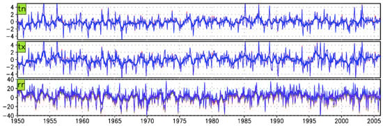
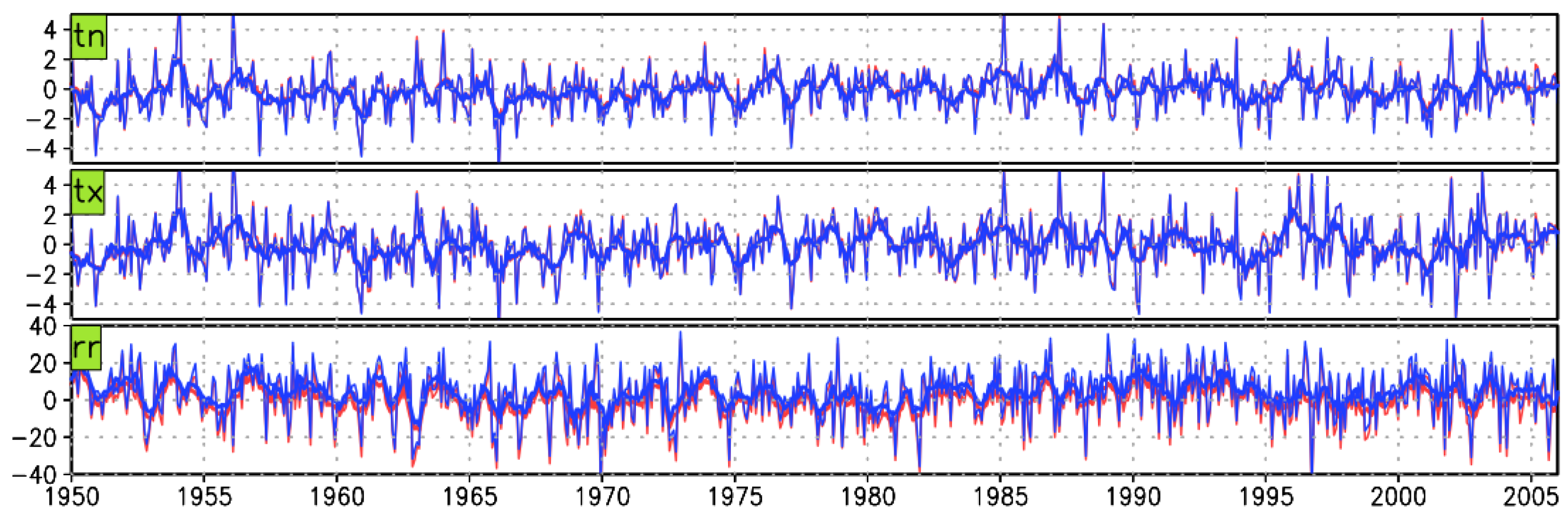
Figure 1.
BIAS of the MX50 (red line) and MMM (blue line) of tn, tx (units: °C), and rr (unit: mm). The fat lines are the centered 7-months running mean.
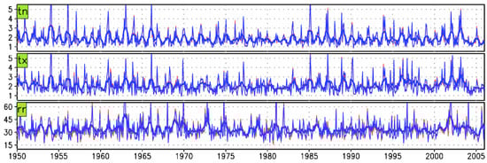
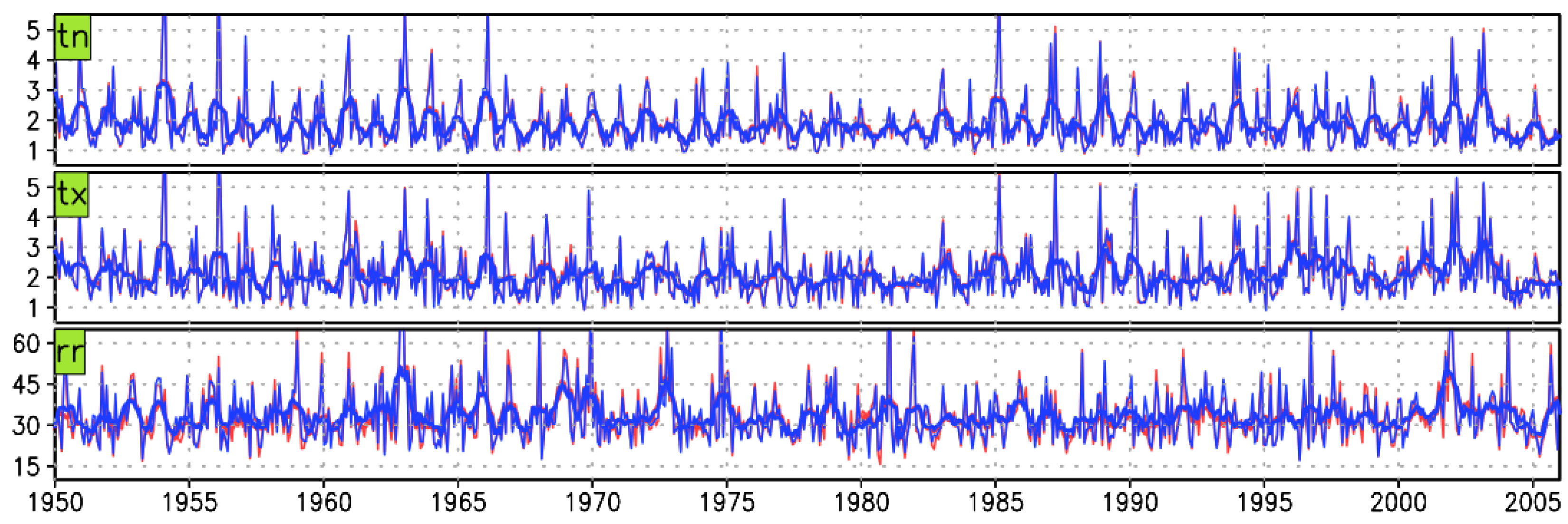
Figure 2.
Same as Figure 1 but for the RMSE.
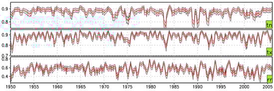
Figure 3.
Correlation of the MX50 of tn, tx, and rr. The red lines are the centered 7-months running mean and the shading shows the 95% confidence interval of the corr.
The overall first impression from Figure 1, Figure 2 and Figure 3 is that the time evolution of the BIAS, RMSE, and corr for the MX50 and the MMM are practically identical. The quantitative aspect will be commented in the next paragraph.
The spatial distribution of the considered metrics is also important.
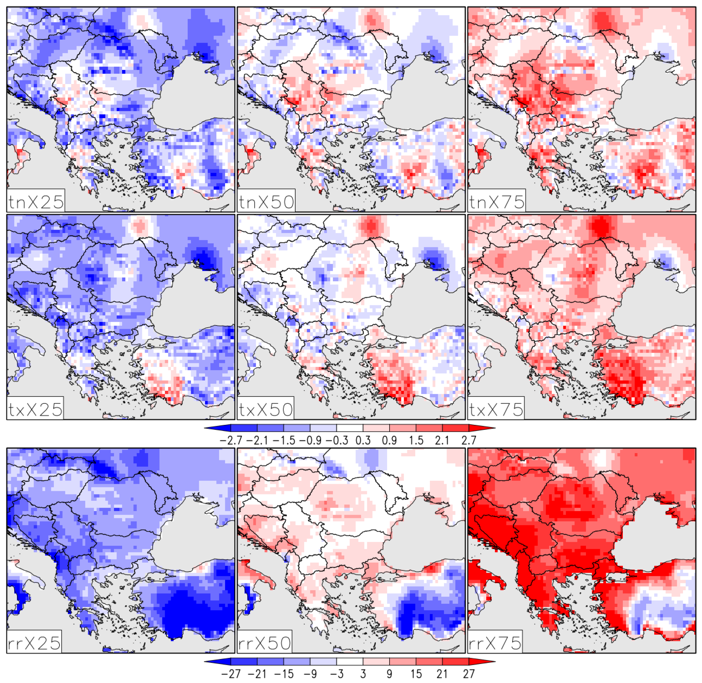
Figure 4 shows the spatial distribution of the biases of the X25, X50 and X75 of the considered parameters in respect to the reference.
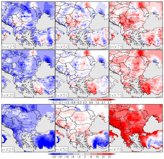
Figure 4.
BIAS of the X25, X50 and X75 of the considered parameters. The units are the same as in Figure 1.
First and foremost, the biases of all parameters of the lower quartile (X25) are predominantly negative and, vice versa, the biases of the upper quartile (X75)—positive. The biases of the medians (X50s) are, compared with those for the X25 and X75, with the generally smallest absolute value. This fact, together with the former two findings, indicates that the reference is, as a whole, in the interquartile interval, closest to the median. Such optimal behavior could be judged as evidence of the ability of the MM ensemble to reproduce the historical climate.
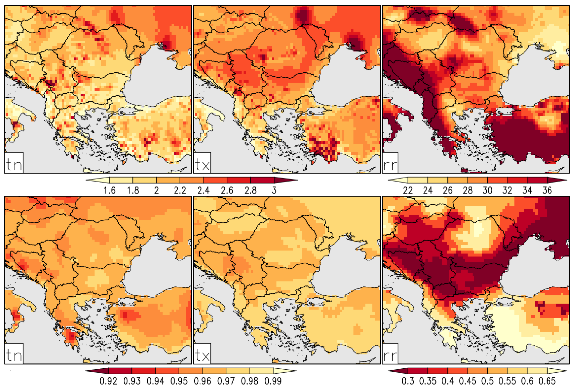
We present also the maps of the RMSE and corr over time (Figure 5) but, for sake of brevity, of the MX50 only.
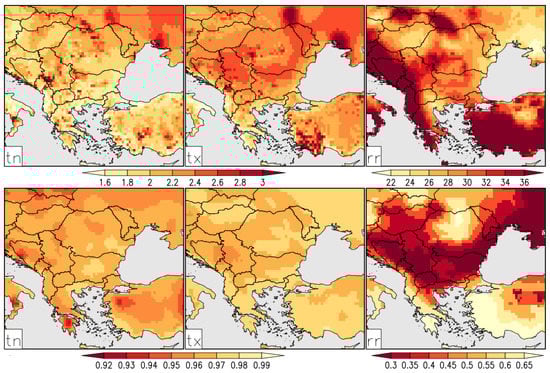
The maps in Figure 5 demonstrate that there are no principal differences for the tn and tx, neither in magnitude nor in the spatial distribution. The statistical metrics of the extreme temperatures are relatively uniformly distributed across the domain, without clear spatial patterns. The overall picture of the evaluation of the monthly precipitation sum is rather different. Generally, the degree of disagreement between the NEX-GDDP ensemble and the reference, expressed in the values of the considered measures, is bigger. A common conclusion of many evaluation studies is that the thermal conditions are generally better than the precipitation simulated both in the GCMs [9,30] and the RCMs [8,12,29]. According to the BIAS, the NEX-GDDP ensemble slightly overestimates the monthly precipitation sum over the bigger part of the domain. Conversely, significant underestimation is detected over Asia Minor. It should be kept in mind, however, that the E-OBS shows also considerable issues over this region. The spatial distributions of the RMSE and corr for the precipitation are more heterogeneous than the corresponding fields of the extreme temperatures. Some local effects could be also outlined as, for example, the relatively high RMSE (over 30 mm) and relatively low (below 0.4) corr over the Dinaric Alps.
Concluding this section, we provide also the time mean values of the considered metrics calculated over the grid space (left section) and spatial means of the calculated over time. These values, listed in Table 1 give a consolidated overall impression of the magnitude of the disagreement of the NEX-GDDP ensemble XMM and X50 from the reference.

Table 1.
Time mean values of the considered metrics calculated over the grid space (left section) and spatial means of of the calculated over the time (right section).
Generally, the correlation coefficients for the extreme temperatures are very high. The RMSE for these two variables is around 2 °C and the BIAS is practically negligible. There are no significant differences in the results for tn and tx on the one hand and in the results for XMM and X50 on the other. As expected, the values of the statistical metrics for the rr are essentially higher than their counterparts for the extreme temperatures. The mean RMSE is close to 33 mm. Significant differences for both ensemble characteristics, XMM and X50, except for the BIAS, are also absent.
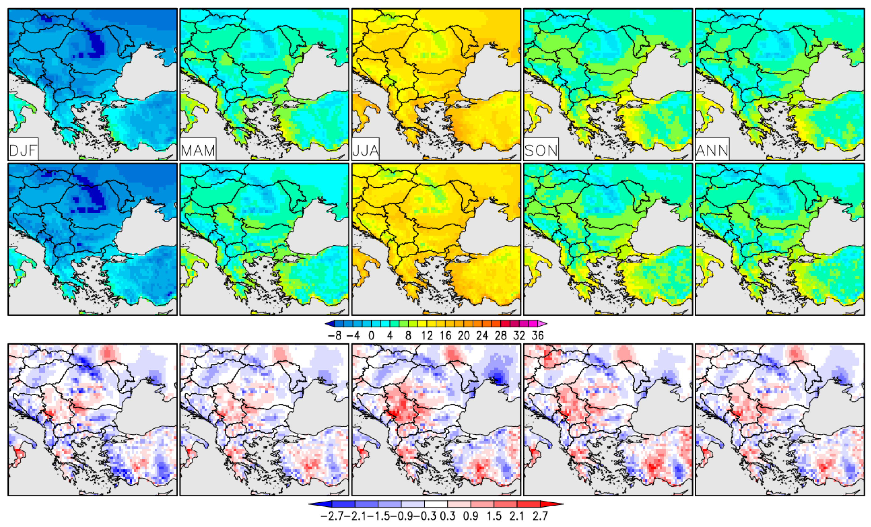
Traditional methods for evaluating the models’ ability to reproduce regional climatic conditions include the statistical analysis of seasonal and annual mean fields and mean error fields relative to the reference measurements [9]. We present validation for the mean tn, tx, and rr (Figure 6, Figure 7 and Figure 8) but for sake of brevity for the MX50 only. With the intention to make the comparison of Figure 6 and Figure 7 easier, the same color legend is used.
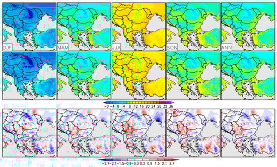
Figure 6.
Multiyear seasonal and annual mean values (units: °C) of tn from E-OBS, NEX-GDDP ensemble as well as the absolute bias (model-reference) on the first, second and third row, respectively.
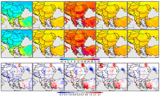
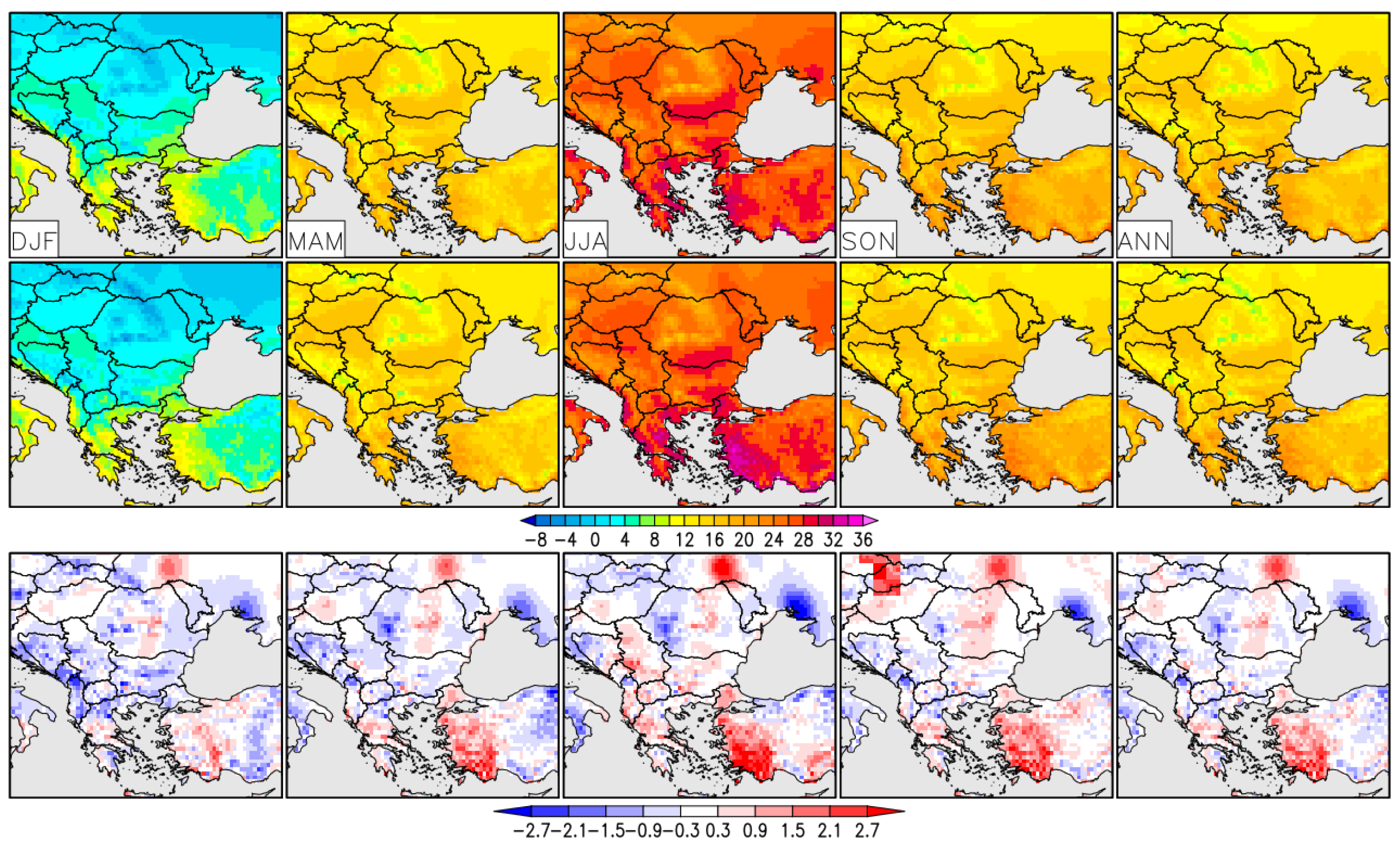
Figure 7.
Same as Figure 6 but for tx.
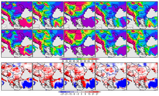
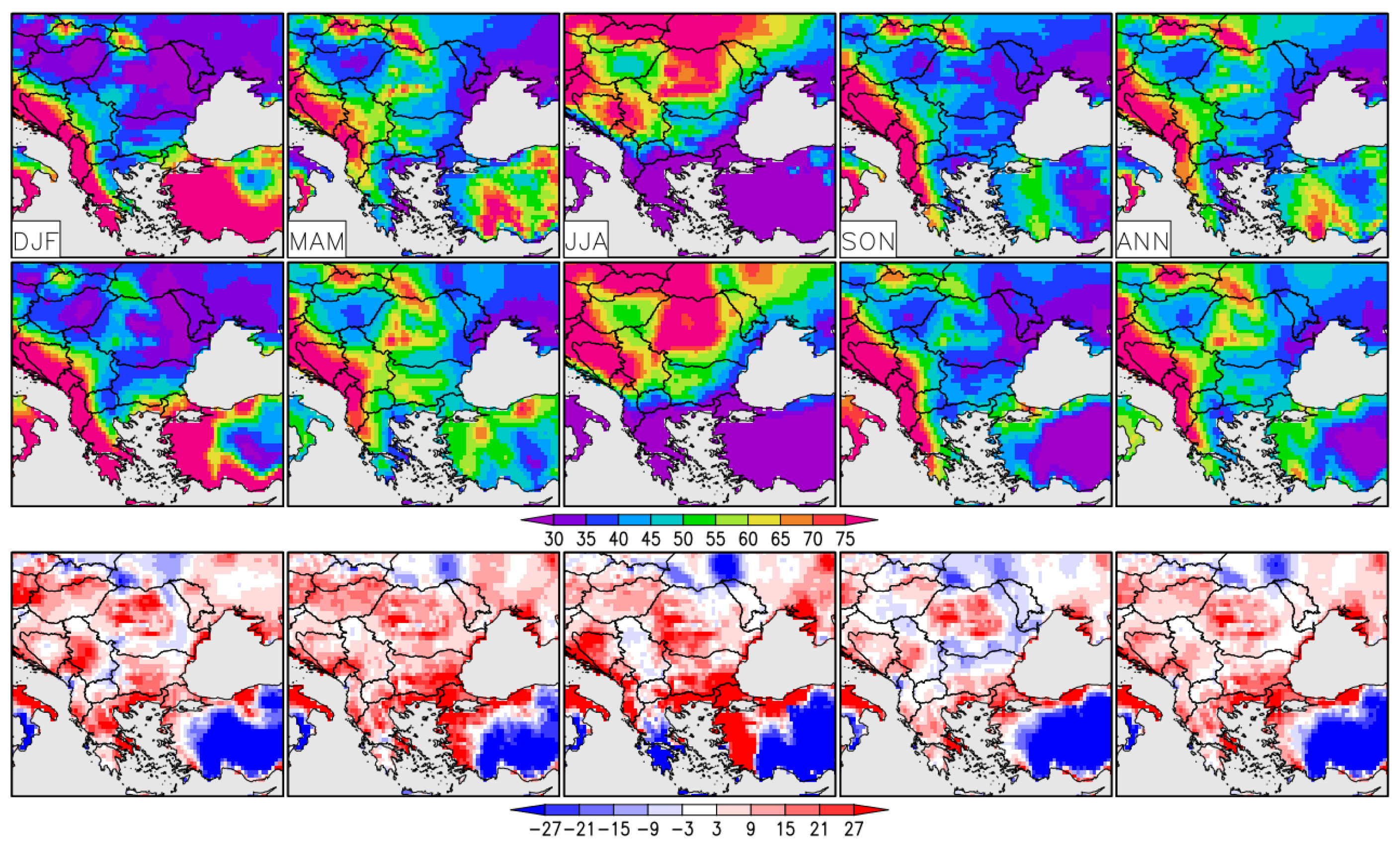
Figure 8.
Same as Figure 6 but for rr (units: mm). Relative (in %) instead of absolute bias is presented.
Generally and most importantly, the magnitude and spatial distribution of the reference data of the extreme temperatures is very well reproduced from the models’ ensemble. Another important outcome is the detected absence of principal difference in the overall picture for the tn on the one hand and the tx on the other. The absolute bias for both temperatures is between −1.5 °C and 1.5 °C over the bigger part of the model domain, except for some isolated regions. The bias does not demonstrate also significant inter-seasonal change. The validation of the multiyear mean seasonal and annual precipitation sum indicates, first of all, spatially prevailing positive bias. It is most prominent in the summer and can also be identified in the other seasons, but is less emphasized. There are also some hot spots of clearly expressed dry bias; the most noticeable, both in magnitude and spatial extent, is over the bigger part of Asia Minor. The latter, however, could be partially explained by the problematic representation of the precipitation in E-OBS over this region, mentioned above.
Many recent studies agree on the fact that the NEX-GDDP ensemble describes very well the mean climate state. According to the extreme temperatures, in [3] is found that the NEX-GDDP successfully reproduces the 1980–2005 averaged climatology of the minimum temperature in January, the maximum temperature in July, and the precipitation rate in July over China. The precipitation sum in July is more consistent with the observations than CMIP5 GCMs. In [21], is noted that the NEX-GDDP data, as compared to the CORDEX and CMIP5, shows a substantial improvement in the precipitation biases over India. The key message in ref. [22] is that the NEX-GDDP data can simulate the Indian summer monsoon rainfall pretty well in comparison to the observation.
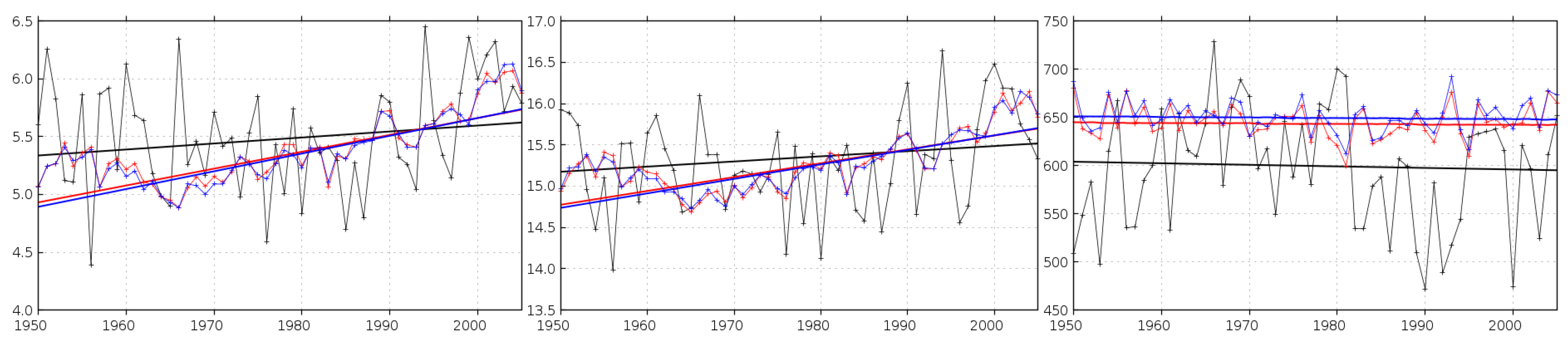
To examine the extent up to which the NEX-GDDP ensemble captures the inter-annual variability and trend of the tn, tx, and rr, the area-weighted average (AAs) values are first calculated over the whole domain applying the E-OBS land-sea mask and then timely aggregated on annual basis. Next, the linear trend magnitude and the p-value of the statistical significance are computed. Figure 9 shows the time series of the AAs of the annual mean tn and tx; the annual rr from the reference data on the one hand and from the NEX-GDDP ensemble MX50 and MMM on the other as well as the corresponding trend lines.
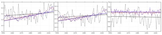
Figure 9.
Time series of the AAs of the annual mean tn (on left, unit: °C), mean tx (in the midle, unit: °C), and rr (unit: mm) as well as the corresponding trend lines from E-OBS (black), NEX-GDDP ensemble MX50 (red), and MMM (blue).
Figure 9 demonstrates, first of all, that the modelled inter-annual variability is significantly lower than the estimated from the reference. The multi-year mean precipitation sum is bigger than the E-OBS estimation which is in coherence with outcomes from the previous paragraph shown in Figure 8. The values of the linear trend magnitude and the p-value of the statistical significance are listed in Table 2 but for sake of brevity for NEX-GDDP ensemble MX50 only.
Table 2.
Trend magnitudes and p-values of the time series of the annual AAs from E-OBS (upper section) and NEX-GDDP ensemble MX50 (lower section). Changes that are not significant at the 5% significance level are bolded.
Table 2 shows that the NEX-GDDP ensemble reproduces correctly the sign of the general tendency, but not the trend magnitude and, for the extreme temperatures, the degree of statistical significance. The trend magnitude of the ensemble MX50 is for all variables approximately three times bigger and for the extreme temperatures statistically significant at the 5% level.
Summarizing the result of previous studies, in [21] is stated that the simulation of trends in the CMIP5 models over India is even poor than the climatological means both in magnitude as well as in distribution. In the same study is found also that the all-India AAs summer mean temperatures are underestimated from the NEX-GDDP ensemble and significantly bigger trend magnitude.
An essential part of the evaluation of single or ensemble models’ performance is to investigate its ability to reproduce the climate extremes, quantified with higher-order statistics, and the tails of the distribution function of the considered variables [9,29]. Therefore, we selected some key ETCCDI climate indices to study the exceedance of given thresholds and duration of specific phenomena. For evaluation of the extreme thermal conditions we use the threshold indices annual occurrence of frost days (FD) and annual occurrence of summer days (SU); the percentile-based indices occurrence of cold nights (TN10p), occurrence of warm days (TX90p); the duration index growing season length (GSL). The definitions of these indicators can be found in [33], for sake of brevity, we will skip them here. Figure 10 shows the comparison of the multiyear means of these indices based on the E-OBS on the one hand and the NEX-GDDP ensemble on the other.
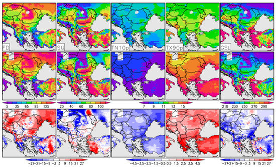
Figure 10.
Multiyear annual mean values of the temperature-based indices from E-OBS, NEX-GDDP ensemble MX50 as well as the absolute bias (model-reference) in the first, second and third row, respectively. The units of the FD, SU, and GSL are days, TN10p and TX90p are expressed in %.
The analysis of Figure 10 indicates that the spatial structures of temperature index values are reproduced satisfactory as a whole. The ensemble generally overestimates the FD and, although weaker, underestimates the SU as well as the GSL. This result is caused by the long-term course of the underlying variables, namely tn for the FD and tx for the SU. Thus, similarities to the multiyear winter bias of the tn (Figure 6) could be found: colder, therefore overestimated FD in the bigger part of the domain. Similarly, the hot spots of positive bias of the tx over east Ukraine and Turkey as well as negative bias over the north Black Sea coast (Figure 7) coincide with the regions with well noticeable bias with the same sign of SU in Figure 10. Spatially the biases of the cold nights (TN10p) and the warm days (TX90p) are most consistent. At first sight, the negative bias of TN10p contradicts to the positive of the FD and, vice versa, the positive bias of TX90p contradicts to the generally negative bias of the SU. It should be kept in mind, however, that the percentile thresholds, used in the calculation of the ensemble-based indices, are computed from the time series of the models’ ensemble, rather than the reference data.
Extreme precipitation is another strong indicator that links regional climate change to people’s daily activities, agricultural plans, and disaster prevention [3]. To investigate the daily precipitation extremes, we have considered the maximum 1-day precipitation amount (RX1day), number of heavy precipitation days greater than 10 mm (R10mm), consecutive dry days (CDD), consecutive wet days (CWD), and very wet days (R95p), (see [33] again). RX1day is an absolute index (it represents maximum precipitation within the year), R10mm is a threshold index, and the R95p is a percentile-based index. CDD, as well as the CWD, are duration indices. All of them are frequently used in many studies conducted at different spatial scales, from planetary to continental, regional, and local scales [11,29]. Similar to Figure 10, Figure 11 shows the comparison of the multiyear means of these indices based on the E-OBS on the one hand and the NEX-GDDP ensemble on the other.
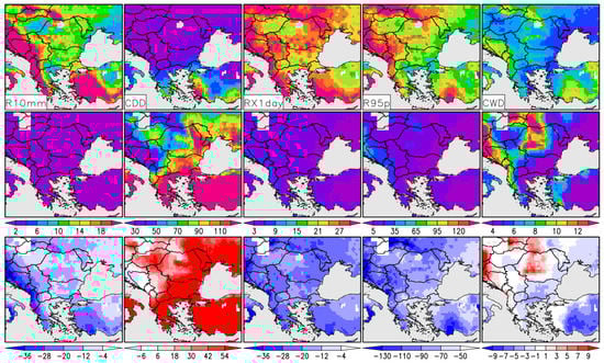
Figure 11.
Multiyear annual mean values of the precipitation-based indices from E-OBS, NEX-GDDP ensemble MX50 as well as the absolute bias (model-reference) on the first, second and third row, respectively. The units of the R10mm, CDD, and CWD are days; of the RX1day and R95p are mm.
The overall and most important outcome from the analysis of Figure 11 is the significant disagreement, both in magnitude and spatial distribution, between the simulation and reference. The NEX-GDDP ensemble considerably underestimates everywhere the R10mm, RX1day, and R95p as well as the CWD over the bigger part of the model domain. Contrarily, the CDD is essentially overestimated. Obviously, the NEX-GDDP ensemble can not adequately reproduce the number of high-intensity events and the precipitation sums during them or, in other words, the simulation fails in the description of the upper tail of the precipitations’ distribution. This fact is illustrated by the histograms of the AAs daily precipitation sum the whole period 1950–2006 from E-OBS on the one hand and from the NEX-GDDP ensemble on the other hand, as shown in Figure 12.
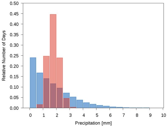
Figure 12.
Relative (in respect to full time span) number of days with rr in the corresponding bin of E-OBS (blue) and NEX-GDDP ensemble (red).
Figure 12 shows how different are the distribution patterns of the daily precipitation sum from E-OBS on the one hand and from the NEX-GDDP ensemble on the other hand. Nearly 95% of the modelled daily precipitation falls in the narrow interval 1.5–3.0 mm and cases with relatively heavy (i.e., >10 mm) precipitation, as shown also in Figure 11, are practically absent. The NEX-GDDP ensemble demonstrates also a very small relative number of cases on the other tail of the distribution, i.e., days with 0.0–0.5 mm.
The latter could be attributed to the special measurements for preventing the so-called “drizzling effect” in the modern GCMs.
The evaluation studies of the performance of the NEX-GDDP ensemble at daily scales documents mixed, partially contradicting results. One of the key messages in [23] is that over South Asia, NEX-GDDP-simulated daily rainfall statistics are not close to observation. Similar to our findings, in [23] is emphasized, that NEX-GDDP fails to capture the observed distributions of the high-intensity rainfall in almost all considered cities and underestimates the rainfall magnitudes. NEX-GDDP also fails to capture the frequencies of dry days when compared to reference data. In [3], is stated, that NEX-GDDP significantly reduces the biases in the climatology of daily total precipitation, in terms of the spatial distribution and extremes across China. In [21], is concluded, that the occurrence of temperature and precipitation extremes is captured realistically in NEX-GDDP data for the reference period over India, and therefore the dataset has great potential for studies related to climate extremes and climate change impact assessment.
4. Conclusions
In the present study, the applicability of the multimodel ensemble, based on NASA’s new bias-corrected NEX-GDDP dataset, has been evaluated for SE Europe for the 56 years long historical period 1950–2006. Most generally, the NEX-GDDP multimodel ensemble reproduces very well the mean climatological state. Overall, NEX-GDDP data represents well the means of the extreme temperatures as well as the precipitation sum on a monthly scale.
The multiyear mean ensemble median for all of the considered essential climate variables is close to the reference of the ground measurements and the spatial distribution of the BIAS shows that the reference is bracketed in the interquartile interval of the ensemble over the bigger part of the considered domain, evidencing the skill of the ensemble to reproduce the historical climate. This key message reflects the most significant result of our study. In general, there is no principal difference of the spatio-temporal patterns of disagreement between the MM ensemble and the reference for the minimum temperature on the one hand and for the maximum temperature on the other.
The evaluation on a daily scale, especially in terms of CIs-assessed extremes, as well as the ensembles’ skill to simulate the long-term trend, shows considerable limitations. This finding is most clearly expressed for the daily precipitation—despite bias-corrected data, NEX-GDDP severely underestimates observations in terms of 1-day maximum, number of heavy precipitation days, 95th percentile rainfalls. As emphasized in [23], this might result in a lot of uncertainties in interpreting future plausible changes. Our findings show that the extreme values of precipitation are subject to high scrutiny when NEX-GDDP data could be applied for further impact studies or in policy-making. The uncertainties in the NEX-GDDP datasets could be linked to several factors but the most probable is the insufficient data from the ground measurements used in the BCSD procedure.
The study could be extended in many directions, in particular, addressing more specific aspects of the historical climate of the region as well as more deeply the properties of the NEX-GDDP MM-ensemble. The insufficiency of regional measurement data, included in the BCSD procedure appears to play key role in the overall data quality deterioration, subsequently for disagreement with the reference. Thus, it is expected that the successors of NEX-GDDP would try to address this problem in the future considering updated records with denser spatial coverage in the BCSD procedure.
The logical continuation of the study is to use the NEX-GDDP ensemble for a comprehensive assessment of the projected future changes in precipitation and extreme temperatures in the region up to the end of the century. Based on the present results, it could be concluded that NEX-GDDP has the potential to become a multi-purpose high-resolution dataset for future regional projections and for other climate change-related studies. Any end-user or policy-maker, however, should understand the limitations and uncertainties that come along before using it for their study which warrants correct evaluations.
Author Contributions
Conceptualization, Methodology, Validation, Formal Analysis, H.C.; Software, K.S. and H.C.; supervision, K.S.; Writing—original draft preparation, H.C.; Writing—review and editing, K.S. All authors have read and agreed to the published version of the manuscript.
Funding
This research was not funded.
Institutional Review Board Statement
Not applicable.
Informed Consent Statement
Not applicable.
Data Availability Statement
The original NEX-GDDP data are downloaded from the NASA data portal: ftp://ftp.nccs.nasa.gov/NEX-GDDP, accessed on 10 November 2021.
Acknowledgments
We acknowledge the contribution of Climate Analytics Group and NASA Ames Research Center using the NASA Earth Exchange, and the NASA Center for Climate Simulation (NCCS) for the NEX-GDDP dataset. Personal thanks to I. Tsonevsky from European Centre for Medium-Range Weather Forecasts for the cooperation. Not at least we thank to the three anonymous reviewers for their valuable comments and suggestions which led to an overall improvement of the original manuscript.
Conflicts of Interest
The authors declare no conflict of interest.
References
- Taylor, K.E.; Stouffer, R.J.; Meehl, G.A. An overview of CMIP5 and the experiment design. Bull. Am. Meteorol. Soc. 2012, 93, 485–498. [Google Scholar] [CrossRef] [Green Version]
- Xue, Y.; Janjic, Z.; Dudhia, J.; Vasic, R.; De Sales, F. A review on regional dynamical downscaling in intraseasonal to seasonal simulation/prediction and major factors that affect downscaling ability. Atmos. Res. 2014, 147–148, 68–85. [Google Scholar] [CrossRef] [Green Version]
- Bao, Y.; Wen, X. Projection of China’s Near- and Long-term Climate in a New High-resolution Daily Downscaled Dataset NEX-GDDP. J. Meteorol. Res. 2017, 31, 236–249. [Google Scholar] [CrossRef]
- Hewitt, C.D.; Griggs, D. Ensembles-Based Predictions of Climate Changes and Their Impacts. Eos Trans. AGU 2004, 85, 566. [Google Scholar] [CrossRef]
- Halenka, T. CECILIA—EC FP6 Project on the Assessment of Climate Change Impacts in Central and Eastern Europe. In Global Environmental Change: Challenges to Science and Society in Southeastern Europe; Alexandrov, V., Gajdusek, M.F., Knight, C.G., Yotova, A., Eds.; Springer: Dordrecht, The Netherlands, 2010; pp. 125–137. [Google Scholar] [CrossRef]
- Jacob, D.; Petersen, J.; Eggert, B.; Alias, A.; Christensen, O.B.; Bouwer, L.M.; Braun, A.; Colette, A.; Déqué, M.; Georgievski, G.; et al. EURO-CORDEX: New high-resolution climate change projections for European impact research. Reg. Environ. Chang. 2014, 14, 563–578. [Google Scholar] [CrossRef]
- Ruti, P.M.; Somot, S.; Giorgi, F.; Dubois, C.; Flaounas, E.; Obermann, A.; Dell’Aquila, A.; Pisacane, G.; Harzallah, A.; Lombardi, E.; et al. MED-CORDEX initiative for Mediterranean Climate studies. Bull. Am. Meteorol. Soc. 2016, 97, 1187–1208. [Google Scholar] [CrossRef] [Green Version]
- Gadzhev, G.; Ivanov, V.; Valcheva, R.; Ganev, K.; Chervenkov, H. HPC Simulations of the Present and Projected Future Climate of the Balkan Region. In Proceedings of the Advances in High Performance Computing (HPC19), Borovets, Bulgaria, 2–6 September 2019; Dimov, I., Fidanova, S., Eds.; Studies in Computational Intelligence, 902. Springer: Cham, Switzerland, 2021; pp. 234–248. [Google Scholar] [CrossRef]
- Pieczka, I.; Bartholy, J.; Pongrácz, R.; André, K.S. Validation of RegCM regional and HadGEM global climate models using mean and extreme climatic variables. IDŐJÁRÁS 2019, 123, 409–433. [Google Scholar] [CrossRef]
- Chervenkov, H.; Slavov, K. Historical Climate Assessment of Temperature-based ETCCDI Climate Indices Derived from CMIP5 Simulations. Comptes Rendus Acad. Bulg. Sci. 2020, 73, 784–790. [Google Scholar] [CrossRef]
- Chervenkov, H.; Slavov, K. Historical Climate Assessment of Precipitation-based ETCCDI Climate Indices Derived from CMIP5 Simulations. Comptes Rendus Acad. Bulg. Sci. 2020, 73, 942–948. [Google Scholar] [CrossRef]
- Kotlarski, S.; Keuler, K.; Christensen, O.B.; Colette, A.; Déqué, M.; Gobiet, A.; Goergen, K.; Jacob, D.; Lüthi, D.; van Meijgaard, E.; et al. Regional climate modeling on European scales: A joint standard evaluation of the EURO-CORDEX RCM ensemble. Geosci. Model Dev. 2014, 7, 1297–1333. [Google Scholar] [CrossRef] [Green Version]
- Thrasher, B.; Xiong, J.; Wang, W.; Melton, F.; Michaelis, A.; Nemani, R. Downscaled Climate Projections Suitable for Resource Management. Eos Trans. AGU 2013, 94, 321. [Google Scholar] [CrossRef]
- Thrasher, B.; Maurer, E.P.; McKellar, C.; Duffy, P.B. Technical note: Bias correcting climate model simulated daily temperature extremes with quantile mapping. Hydrol. Earth Syst. Sci. 2012, 16, 3309–3314. [Google Scholar] [CrossRef] [Green Version]
- Chadalavada, K.; Gummadi, S.; Kundeti, K.R.; Kadiyala, D.M.; Deevi, K.C.; Dakhore, K.K.; Bollipo Diana, R.K.; Thiruppathi, S.K. Simulating Potential Impacts of Future Climate Change on Post-Rainy Season Sorghum Yields in India. Sustainability 2022, 14, 334. [Google Scholar] [CrossRef]
- Wood, A.W.; Maurer, E.P.; Kumar, A.; Lettenmaier, D.P. Long-range experimental hydrologic forecasting for the eastern United SP. J. Geophys. Res. Atmos. 2002, 107, 1–15. [Google Scholar] [CrossRef]
- Wood, A.W.; Leung, L.R.; Sridhar, V.; Lettenmaier, D.P. Hydrologic Implications of Dynamical and Statistical Approaches to Downscaling Climate Model Outputs. Clim. Chang. 2004, 62, 189–216. [Google Scholar] [CrossRef]
- Ali, J.; Syed, K.H.; Gabriel, H.F.; Saeed, F.; Ahmad, B.; Bukhari, S.A.A. Centennial Heat Wave Projections Over Pakistan Using Ensemble NEX GDDP Data Set. Earth Syst. Environ. 2018, 2, 437–454. [Google Scholar] [CrossRef]
- Cao, N.; Li, G.; Rong, M.; Yang, J.; Xu, F. Large Future Increase in Exposure Risks of Extreme Heat within Southern China Under Warming Scenario. Front. Earth Sci. 2021, 9. [Google Scholar] [CrossRef]
- Luo, Z.; Yang, J.; Gao, M.; Chen, D. Extreme hot days over three global mega-regions: Historical fidelity and future projection. Atm. Sci. Lett. 2020, 21, e1003. [Google Scholar] [CrossRef]
- Jain, S.; Salunke, P.; Mishra, S.K.; Sahany, S.; Choudhary, N. Advantage of NEX-GDDP Over CMIP5 and CORDEX Data: Indian Summer Monsoon. Atmos. Res. 2019, 228, 152–160. [Google Scholar] [CrossRef]
- Kumar, P.; Kumar, S.; Barat, A.; Sarthi, P.P.; Sinha, A.K. Evaluation of NASA’s NEX-GDDP-simulated summer monsoon rainfall over homogeneous monsoon regions of India. Theor. App. Clim. 2020, 141, 525–536. [Google Scholar] [CrossRef]
- Raghavan, S.V.; Hur, J.; Liong, S.-Y. Evaluations of NASA NEX-GDDP data over Southeast Asia: Present and future climates. Clim. Chang. 2018, 148, 503–518. [Google Scholar] [CrossRef]
- Cornes, R.; van der Schrier, G.; van den Besselaar, E.J.M.; Jones, P.D. An Ensemble Version of the E-OBS Temperature and Precipitation Datasets. J. Geophys. Res. Atmos. 2018, 123, 9391–9409. [Google Scholar] [CrossRef] [Green Version]
- Chervenkov, H.; Slavov, K. Theil–Sen Estimator vs. Ordinary Least Squares—Trend Analysis for Selected ETCCDI Climate Indices. Comptes Rendus Acad. Bulg. Sci. 2019, 72, 47–54. [Google Scholar] [CrossRef]
- Bandhauer, M.; Isotta, F.; Lakatos, M.; Lussana, C.; Båserud, L.; Izsák, B.; Szentes, O.; Tveito, O.E.; Frei, C. Evaluation of daily precipitation analyses in E-OBS (v19.0e) and ERA5 by comparison to regional high-resolution datasets in European regions. Int. J. Climatol. 2021, 42, 727–747. [Google Scholar] [CrossRef]
- Herger, N.; Abramowitz, G.; Knutti, R.; Angélil, O.; Lehmann, K.S.; Sanderson, B.M. Selecting a climate model subset to optimise key ensemble properties. Earth Syst. Dynam. 2018, 9, 135–151. [Google Scholar] [CrossRef] [Green Version]
- Knutti, R. The end of model democracy? Clim. Chang. 2010, 102, 395–404. [Google Scholar] [CrossRef]
- Torma, C.Z. Detailed validation of EURO-CORDEX and Med-CORDEX regional climate model ensembles over the Carpathian Region. IDŐJÁRÁS 2019, 123, 217–240. [Google Scholar] [CrossRef]
- Gleckler, P.J.; Taylor, K.E.; Doutriaux, C. Performance metrics for climate models. J. Geophys. Res.-Atmos. 2008, 113, D06104. [Google Scholar] [CrossRef]
- Chervenkov, H.; Ivanov, V.; Gadzhev, G.; Ganev, K. Assessment of the Future Climate over Southeast Europe Based on CMIP5 Ensemble of Climate Indices—Part Two: Results and Discussion. In Proceedings of the 1st International Conference on Environmental Protection and Disaster RISKs, Sofia, Bulgaria, 29–30 September 2020; Gadzhev, G., Dobrinkova, N., Eds.; pp. 157–169. [Google Scholar] [CrossRef]
- Sillmann, J.; Kharin, V.V.; Zhang, X.; Zwiers, F.W.; Bronaugh, D. Climate extremes indices in the CMIP5 multimodel ensemble: Part 1. Model evaluation in the present climate. J. Geophys. Res. Atmos. 2013, 118, 1716–1733. [Google Scholar] [CrossRef]
- Zhang, X.; Alexander, L.; Hegerl, G.C.; Jones, P.; Tank, A.K.; Peterson, T.C.; Trewin, B.; Zwiers, F.W. Indices for monitoring changes in extremes based on daily temperature and precipitation data. WIREs Clim. Chang. 2011, 2, 851–870. [Google Scholar] [CrossRef]
- Sen, P.K. Estimates of the regression coefficient based on Kendall’s tau. J. Am. Stat. Assoc. 1968, 63, 1379–1389. [Google Scholar] [CrossRef]
- Theil, H. A rank-invariant method of linear and polynomial regression analysis. I, II, III. Nederl. Akad. Wetensch. Proc. 1950, 53, 386–392, 521–525, 1397–1412. [Google Scholar]
- Kendall, M.G. A new measure of rank correlation. Biometrika 1938, 30, 81–93. [Google Scholar] [CrossRef]
- Mann, H.B. Nonparametric tests against trend. Econometrica 1945, 13, 245–259. [Google Scholar] [CrossRef]
- WMO. Detecting Trend and Other Changes in Hydrological Data; WCDMP-45, WMO/TD 1013; WMO: Geneva, Switzerland, 2000. [Google Scholar]
- Schulzweida, U. CDO User Guide (Version 2.0.0). 30 October 2020. Available online: https://zenodo.org/record/5614769#.Yk027ihBxPY (accessed on 10 November 2021).


Publisher’s Note: MDPI stays neutral with regard to jurisdictional claims in published maps and institutional affiliations. |
© 2022 by the authors. Licensee MDPI, Basel, Switzerland. This article is an open access article distributed under the terms and conditions of the Creative Commons Attribution (CC BY) license (https://creativecommons.org/licenses/by/4.0/).