Wind Speed and Direction Mapping with HF Radar

Highlights

What are the main findings?

• A support vector regression method has been applied to HF radar data from three different radar sites operating at different radio frequencies, trained using the Copernicus European Regional ReAnalysis (CERRA) wind model wind speeds to provide an HF radar wind speed mapping capability.
• The method has been applied to data not used during the training and testing phase, and consistent wind maps are obtained. The statistics of the derived wind speeds compared with the CERRA model are similar to those between the model and in situ winds.

What are the implications of the main finding?

• Wind speed can now be added to the wave, current and wind direction data provided by HF radars from the coast to 10s of km offshore to support many activities in coastal waters, including offshore wind and other renewable energy operations, scientific studies, shipping, leisure activities, metocean predictions using assimilation, etc.
• Suggestions to further improve the method are provided.

Abstract

HF radar systems are used in many parts of the world as a part of operational coastal ocean observing systems. Their primary product is surface current mapping from the coast to a range determined by radio frequency and environmental conditions. Initiatives to promote their use for wave measurement are now being developed. Obtaining reliable wind measurements has proved more difficult primarily because there is no direct physical relationship between the radar signal and the wave field. In this paper, a machine learning approach, previously demonstrated for radar data at the location of an in situ measurement, has been extended to allow for wind mapping using wind model data for training. Using data from three different radar deployments operating at different frequencies, a single machine learning model has been developed that can be applied to all three locations. A subset of the model data is used in the training and testing of the method, and accuracy is assessed using a mix of these data and data at all model positions within the radar field of view. The results show that the new wind speed measurements are significantly more accurate than those previously available using an inverse wind-wave model. Radar wind maps are consistent with, although show more spatial variability than, model or satellite winds. More validation with offshore wind masts is recommended.

1. Introduction

HF radars are normally located on the coast and are routinely used for surface current measurements in many parts of the world [1,2,3,4]. Their use hlfor wave [5] and wind direction [6] measurements has also been demonstrated, although these are not yet as widely available as current measurements. Wind speed measurement is more of a challenge since there is no direct physical relationship with radar backscatter. The local wave field responsible for the scattering is, in part, generated by the local wind, but also depends on the duration and fetch over which the wind has been blowing. It also often includes swell from distant storms. Ref. [7] reviewed a number of methods that use both the first-order and second-order parts of the radar Doppler spectrum to determine the wind speed, but none of these have yet produced a robust estimate with an accuracy useful for operational and scientific applications. A comparison of wind speed accuracies using various methods is given in [8].

Ref. [8] demonstrated the feasibility of using machine learning (ML) methods to obtain wind speeds from HF radar systems. The results obtained, whilst encouraging, were site-specific (for three different sites on the west coast of the UK) in two cases, being valid only at the position of the in situ data used to train the machine learning. In the third case, spatial coverage was possible because model data across the region were available for training. In this study, this work is extended to (a) include additional ML methods, (b) to optimize the parameters of the ML methods, (c) to provide spatial mapping of winds, and (d) to seek a site-independent method. In addition, more data have become available, which will potentially provide more robust training and more general testing data sets. Spatial mapping and radar/site independence are the key innovations of this work.

The data sets used are described in Section 2.1. This is followed by a brief description of the ML methods in Section 2.2. More details are provided in [8]. Since there are no in situ wind measurements spread over the coverage regions of the radars, CERRA model data (see Section 2.1.3) will be used to develop the ML models. Using model data to derive the radar measurement could introduce systematic biases in the estimates due to model limitations. Therefore Section 2.2.1 compares CERRA data at the location of in situ measurements to provide confidence in their use for the radar work. The radar results are presented in Section 3, followed by a discussion and some conclusions, including suggestions for further work.

2. Materials and Methods

2.1. Data Sets

2.1.1. HF Radar

In this paper, the analysis is focused on three sites, Liverpool Bay [9], the South Celtic Sea [10,11] and the North Celtic Sea [12]. In the first two cases, WERA HF radars [13] were deployed for several years. The latter case used Pisces HF radars [14]. Acronyms for these sites used elsewhere in the text are included in brackets in Table 1, where additional dates refer to periods that could be used for further tests. The acronyms are those used in our software for those sites and are used here for consistency with our databases. WERA radars are available from Helzel GmbH, Kaltenkirchen, Germany. Pisces radars are no longer available.

Table 1. Available radar data.

Site	Dates Used for ML	Additional Dates	Frequency
Liverpool Bay (lb)	2005-10-01 00:00 to 2006-02-28 23:002007-09-04 15:00 to 2007-12-31 23:00	2008-01-01 01:00 to 2011-12-01 09:00	12–14 MHz
South Celtic Sea (whc)	2012-03-30 00:15 to 2012-04-27 23:052012-10-26 00:05 to 2013-02-28 23:05	others in range 2011–2025	12–13 MHz
North Celtic Sea (cs)	2003-12-01 21:00 to 2005-06-05 16:00	–	5–15 MHz

Unlike the WERA radar, which provides measurements on a rectangular grid (with a resolution of 3 $\mathrm{k}$$\mathrm{m}$ in Liverpool Bay and 1 $\mathrm{k}$$\mathrm{m}$ in the South Celtic Sea), the Pisces radar, at the time of these measurements, measured on a coarse radial grid of three beam directions sampled sequentially and 20, 15 $\mathrm{k}$$\mathrm{m}$ separation, ranges along these directions from each radar. To obtain dual radar results, the data were combined, with measurements from each radar separated by no more than 18 $\mathrm{k}$$\mathrm{m}$.

WERA and Pisces are phased-array radars that are able to resolve radar signals from small patches of the sea surface, often referred to as cells, determined by the bandwidth of the radar signal and the azimuthal resolution of the radar, which depends on the number of antennae in a usually linear array. The features used in the development of a wind speed algorithm are obtained from the power (Doppler) spectrum of the signal at each cell [8]. Another commonly used radar is the CODAR SeaSonde [15], but this only resolves the radar signal at fixed ranges from the radar site. The azimuthal resolution for surface current measurement can be obtained using direction-finding, but the Doppler data are not suitable for the wind-mapping approach described in this paper.

2.1.2. In Situ

Details of various sources of in situ data are shown in Table 2. The Liverpool Bay mast and Perranporth met station data were used in the development of the original radar algorithm [8]. The M5 buoy is located well outside the radar coverage area but provides useful data to assess the model and satellite winds. In this work, these data are used to validate the model to support its use in the radar wind speed algorithm.

Table 2. Available in situ data.

System	Location	Height	Source	Period
Met Mast Liverpool Bay	53.4792583 N 3.507013 W	25 $\mathrm{m}$	NPower Renewables(now part of E.ON)	05/09/2005 00:00 to 31/01/2008 23:50
Perranporth Gill Met Pack II (on coast)	50.346167 N 5.16183 W	48.36 m	https://www.coastalmonitoring.org/realtimedata/?chart=76 , accessed 16 March 2026.	01/01/2012 00:00 to 31/12/2012 23:50
M5 buoy	51.690425 N 6.704336 W	4.16 m	Irish Marine Institute ERDDAP server	01/10/2010 00:00 to 01/03/2025 00:00
Hilbre Island Anemometer	53.4792583 N 3.507013 W	25 $\mathrm{m}$	https://www.bodc.ac.uk/data/bodc_database/nodb/data_collection/224/ , accessed 20 March 2026.	Only used for qualitativevalidation

2.1.3. Model Data

The model data used to develop the ML algorithm are from the Copernicus European Regional ReAnalysis (CERRA) model [16], (CERRA sub-daily regional reanalysis data for Europe on single levels from 1984 to present, 10 m wind reanalysis using data assimilation, available from https://cds.climate.copernicus.eu, accessed 16 March 2026). The model has a spatial resolution of $5.5$ $\mathrm{k}$$\mathrm{m}$, which is between the resolutions of the two radar systems used in this study, and 3 h temporal resolution. The model uses a three-dimensional variational assimilation scheme (3D-Var) and assimilates many different types of surface and satellite observations [17]. These model data have been compared with other models in [18] and showed better skill at wind speed measurement, particularly in coastal waters, which is where HF radars operate. Figure 1 shows samples of model data and the location of radar measurement cells within 2 $\mathrm{k}$$\mathrm{m}$. These will be used for algorithm development; some for training and testing, and the rest for validation. The different spatial and temporal resolutions of the model compared to the radar means that there are plenty of radar data for further validation unused in the model development.

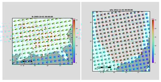
Figure 1. Examples of model wind speed (colour-coded) and direction (arrows) sampling in Liverpool Bay (left) and Wave Hub region (right). Radar measurement cells $·$; within 2 $\mathrm{k}$$\mathrm{m}$ •, some of the latter used for training and others for testing and validation. Radar sites are indicated with ⧫.

2.1.4. Satellite Data

The satellite data used are from ASCAT [19] (L2 Winds Data Record Release 1—Metop available from https://user.eumetsat.int/data-access/data-store, accessed 16 March 2026). This has a spatial resolution of $12.5$ $\mathrm{k}$$\mathrm{m}$. Figure 2 shows samples of satellite data and the location of radar measurement cells within 2 $\mathrm{k}$$\mathrm{m}$. The co-locations vary and are infrequent, so these will be used for qualitative validation and not for the development of the radar wind speed algorithm.

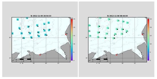
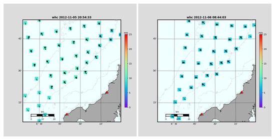
Figure 2. Examples of satellite wind speed (colour-coded) and direction (arrows) sampling in Liverpool Bay (above) and Wave Hub region (below). Radar measurement cells within 2 $\mathrm{k}$$\mathrm{m}$ are shown in •. Radar sites are indicated with ⧫.

2.2. Methods

In [8], a number of different ML methods available in the Python 3.12.3 Sklearn 1.4.1.post1 package [20] were trialed to determine wind speed from the radar data using in situ wind measurements for training and evaluating. It was concluded that the support vector regression method (SVR) gave the best results. The details on the SVR method are given in [8]. The SVR models obtained were different for the different radar sites due to different operating frequencies, water depths and probably other site-specific factors that were included in and/or affect the radar data features used in the model development (see [8] for details). In this study, the aim is to develop a single model that can be used to map winds across different deployments, avoiding the need to train a new model for each new radar or site. Unfortunately, having a number of sources of sea-truth across the radar coverage is not practical, and satellite temporal and spatial sampling does not provide enough data for this work. Therefore, wave model data from a number of locations across the field of view of three different radar systems are used for training and testing ML methods. Comparisons between model winds and in situ winds where they are available are used to give some confidence in the model and provide a baseline to judge the radar measurement accuracy. The method is developed in three stages: (1) at the location of an in situ instrument to compare the use of in situ and model data in the ML methods; (2) at selected model cells for each deployment separately; (3) using model and radar data from all three deployments.

SVR is compared with two methods not used in the previous work: a Sklearn neural network method (Multi-layer Perceptron regressor), denoted as NN, and XGBoost, denoted as XGB [21], and in each case, including SVR, the parameters of the model are optimized using Sklearn RandomizedSearchCV and assessed using Sklearn cross-validation. The optimization was not used in [8]. As discussed later, SVR still gives the best results, although the neural network results are not too different.

In the previous work [8], the radar parameters used in the ML modeling were obtained from the radar Doppler spectra files and from the file generated by the Seaview inversion process (files with extension .sea) as a post-processing step in Python. These parameters are now all calculated during the initialization of the inversion, which outputs them to a netCDF file that is then used in the ML modeling. This makes it possible to implement the selected ML model during the inversion process (see Section 4), thus allowing for much more accurate near-real-time wind speed measurement.

2.2.1. CERRA Model Compared with In Situ Winds

Details about the model are given in Section 2.1.3. These data are compared with the in situ data in this section to provide a baseline for the later radar evaluation.

Liverpool Bay

The comparison in Figure 3 is between the co-located (within $2.5$ $\mathrm{k}$$\mathrm{m}$), co-temporal (with 5 min) model and mast data. The instrument is located 25 $\mathrm{m}$ above sea level and has been adjusted to 10 $\mathrm{m}$ with roughness length $z_0=0.0016$. The correlation coefficient and root-mean-square ($\mathrm{rms}$) values are similar to those that have been found in other work [18], so we consider that there is sufficient agreement to support the use of the model data to train the machine learning methods.

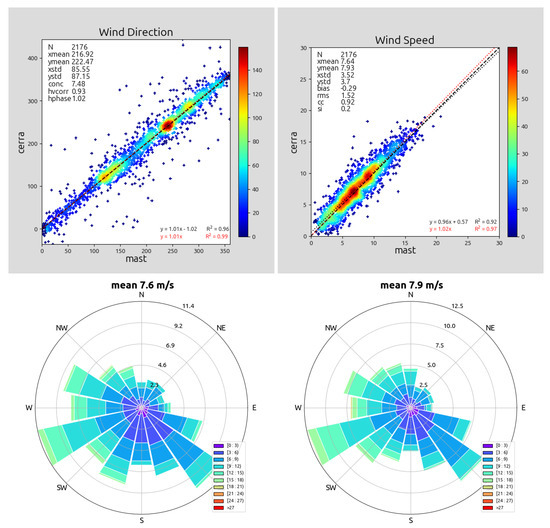
Figure 3. Above: Scatter plots of wind speed (right) and direction (left) in Liverpool Bay. Color coding in this and subsequent scatter plots indicates the density of observations, with the numbers on the color scale indicating the number of cases in close proximity to each point using a smoothed histogram method. The black and red dotted lines are the linear relationships, with and without an intersect, shown in the lower right corner. Below: Wind roses mast (left) model (right).

South Celtic Sea

The comparison in Figure 4 is between the co-located (within 2 $\mathrm{k}$$\mathrm{m}$), co-temporal (with 5 min) model and Coastal Observatory Perranporth met data. The met station is on land close to the coast and probably sheltered from winds from NNE to SW, so it is difficult to select a roughness length, $z_0$, suitable for scaling wind speeds to 10 $\mathrm{m}$ from the instrument height of $48.36$ $\mathrm{m}$. A value of 0.25 has been used here, providing a reasonable correlation with the model winds, but the wind roses show different directional distributions. Filtering the data sets by wind direction to exclude the more sheltered directions improves the comparison somewhat, providing enough confidence to use the model data for machine learning. A better comparison is achieved between the model and the Irish M5 buoy, although located outside the radar coverage area of either South or North Celtic Sea radars. The instrument is located $4.16$ $\mathrm{m}$ above sea level and has been adjusted to 10 m with $z_0=0.0016$. This is shown in Figure 5. This gives more confidence in using the model to train machine learning methods at this location. The statistics of the CERRA comparisons are similar to those in some other studies, e.g., [18], although it is difficult to make absolute comparisons with other work due to differences between models, in scaling to 10 m height, or in the averaging of the in situ winds. The statistics obtained here will be used as a baseline with which to judge the radar results.

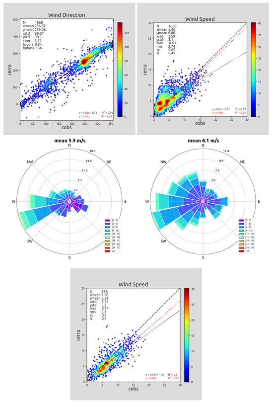
Figure 4. Above: Scatter plots of wind speed (right) and direction (left) in South Celtic Sea. Middle: Wind roses met station (left) model (right). Below: Scatter plot of wind speed after filtering by met station wind direction.

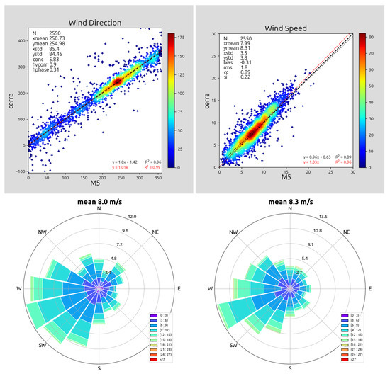
Figure 5. Above: Scatter plots of wind speed (right) and direction (left) at M5 buoy. Below: Wind roses M5 buoy (left) model (right).

Wind speed statistics for both sites are given in Table 3. Included in the statistics are the root-mean-square difference, $\mathrm{rms}$, Pierson correlation coefficient, $\mathrm{cc}$ and scatter index, $\mathrm{si}$, defined as

$$\begin{array}{cc}\hfill \mathrm{rms}& =\sqrt{{\displaystyle \frac{{(x-y)}^2}{N}}}\hfill \\ \hfill \mathrm{cc}& ={\displaystyle \frac{\sum (x-x_{\mathrm{mean}})(y-y_{\mathrm{mean}})}{\sqrt{\sum {(x-x_{\mathrm{mean}})}^2)\sum {(y-y_{\mathrm{mean}})}^2}}}\hfill \\ \hfill \mathrm{si}& =\sqrt{{\displaystyle \frac{{(x-x_{\mathrm{mean}}-(y-y_{\mathrm{mean}}))}^2}{x_{\mathrm{mean}}}}}\hfill \end{array}$$

Table 3. Statistics of CERRA model wind speeds compared to in situ. Units (where relevant) are m/s.

Site	N	x-mean/std	y-mean/std	bias	rms	cc	si
Liverpool Bay	2176	7.64/3.52	7.93/3.70	−0.29	1.52	0.92	0.20
South Celtic Sea (direction filter)	531	7.46/3.48	7.40/3.30	0.06	1.98	0.83	0.27
M5 buoy	2550	7.99/3.50	8.31/3.80	−0.31	1.80	0.89	0.22

3. Results

Models have been developed for the scenarios summarized in Table 4. In each case, the data for the individual sites were split into two by time, with the second half of the data used to train and the first half to test. The wind speed distributions were similar in each half. The number of samples is shown in the table.

Table 4. Model tests.

Model	Model Abbreviation	Liverpool Bay (lb)	South Celtic Sea(whc)	North Celtic Sea(cs)
In situ	in situ, see Section 3.1	mast at 194, train/test samples: 2548/2547	onshore used nearest 6104, samples: 1271/1271	no instrument
CERRA at one radar cell	CERRA, Section 3.1	194, samples: 841/840	6104 samples: 491/490
Single site, CERRA at multiple cells	individual site name as above, Section 3.2.1	11 cells used for train/test, 40 for validation, samples: 9528/9528	27/161, samples: 9194/9194	12/34, samples: 9199/9199
All sites, multiple cells. Statistics calculated for combined sites/cells, validations for all CERRA locations at each site and for individual cells at each site.	3 sites, Section 3.2.2	6 for train/test, 40 CERRA, 194 individual cell, samples: 5130/5132	14/161/4280, samples: 4786/4788	12/34/220, samples: 9198/9200

3.1. Single Cell Results

In Table 5, the results compare all three ML models at the nearest radar cell to the in situ data in Liverpool Bay and the South Celtic Sea using the in situ and CERRA wind speeds. About three times as much Liverpool Bay data were used compared to [8], and the in situ rms values and scatter indices for both training and testing are a little higher, but the correlation coefficients are similar. More data were also used in the South Celtic Sea, with half used for training and half for testing, whereas $90\%$ were used for training in [8]. The XGB results for rms, cc and si are mostly worse than SVR and NN. This is also true for all other cases considered, so no further XGB results will be presented.

Table 5. Statistics of radar wind speeds compared to in situ and CERRA at nearest cell to in situ. Units (where relevant) are m/s.

Site		ML	N	x-mean/std	y-mean/std	bias	rms	cc	si
Liverpool Bay	TRAIN	SVR	2548	8.22/3.65	8.20/3.37	0.02	1.29	0.94	0.16
in situ		NN			8.16/3.37	0.06	1.25	0.94	0.15
		XGB			8.23/3.26	−0.01	1.41	0.92	0.17
	TEST	SVR	2547	7.70/3.26	7.91/2.96	−0.21	1.55	0.88	0.20
		NN			7.80/2.95	−0.1	1.57	0.88	0.20
		XGB			8.06/2.87	−0.36	1.69	0.86	0.21
Liverpool Bay	TRAIN	SVR	841	8.52/3.71	8.48/3.40	0.04	1.19	0.95	0.14
CERRA		NN			8.53/3.46	−0.01	1.18	0.95	0.14
		XGB			8.52/3.25	−0.00	1.35	0.93	0.16
	TEST	SVR	840	8.14/3.46	8.14/3.02	0.00	1.61	0.89	0.20
		NN			8.29/3.37	−0.15	1.74	0.87	0.21
		XGB			8.48/2.94	−0.33	1.81	0.86	0.22
South Celtic Sea	TRAIN	SVR	1271	6.00/3.10	5.90/2.44	0.11	1.63	0.85	0.27
in situ		NN			6.08/3.02	−0.07	1.79	0.82	0.30
		XGB			6.03/2.56	−0.03	1.51	0.88	0.25
	TEST	SVR	1271	5.99/2.79	5.79/2.18	0.19	1.71	0.79	0.28
		NN			5.90/2.49	0.08	1.79	0.78	0.30
		XGB			5.88/2.29	0.11	1.75	0.78	0.29
South Celtic Sea	TRAIN	SVR	491	6.89/3.23	6.72/2.24	0.18	1.20	0.80	0.29
CERRA		NN			6.88/2.56	0.01	1.75	0.84	0.25
		XGB			6.92/2.49	−0.02	1.59	0.88	0.23
	TEST	SVR	490	6.38/2.51	6.22/1.72	0.16	1.85	0.67	0.29
		NN			6.12/2.06	0.25	2.03	0.63	0.32
		XGB			6.56/1.73	−0.18	2.20	0.52	0.34

3.2. Multiple Location Cases

Restricting ML model development to one location limits the applicability of the modeling to similar frequencies, water depths and possibly radar look directions and other site-specific factors. To provide a more general wind speed method, model development was extended to include CERRA data from multiple radar cells for each radar deployment (see Section 2.1.1) and, in addition, combining all radar deployments (see Table 4).

The number of cells used for the ML development had to be limited due to available computer resources. However, this does mean that we have data at locations not used in the modeling that can be used for further testing. The cells used for each case are shown in Figure 6. For Liverpool Bay, the cells were subsampled by eye since their distribution was not uniform. The same is true for the North Celtic Sea. For the South Celtic Sea, they were subsampled with a requirement that there is at least 12 $\mathrm{k}$$\mathrm{m}$ ( 18 $\mathrm{k}$$\mathrm{m}$ when using all sites) separation between selected cells.

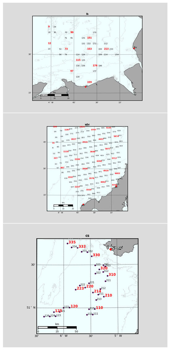
Figure 6. Radar measurement cells within 2 $\mathrm{k}$$\mathrm{m}$ of model grid (see Figure 1), with cells used for individual site ML labeled in bold red. Top: Liverpool Bay, middle: South Celtic Sea, bottom: North Celtic Sea. The Liverpool Bay mast is at cell number 194, and the Perranporth Anemometer is near cell number 5745 on the coast. The M5 buoy is to the NW of both Celtic Sea maps. Radar sites are indicated with ⧫.

3.2.1. Cases 1 to 3: Individual Radar Sites

ML SVR and NN models are obtained using training data for each radar site. Scatter plots for train and test cases for each site are shown in Figure 7, Figure 8 and Figure 9 and statistics are presented in Table 6.

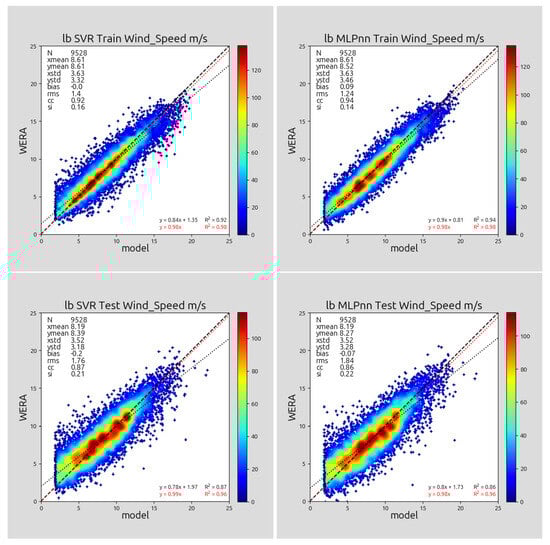
Figure 7. Above: Scatter plots for Liverpool Bay. Training cases for SVR: NN above, testing cases below.

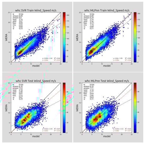
Figure 8. Above: Scatter plots for South Celtic Sea. Training cases for SVR; NN above, testing cases below.

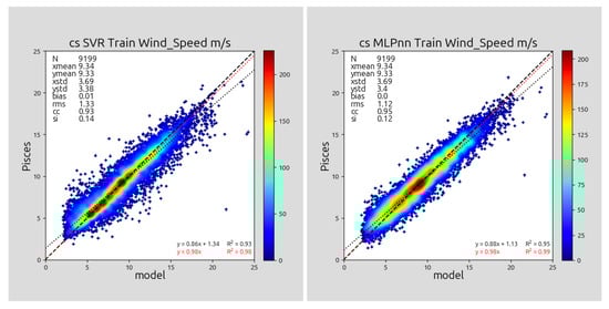
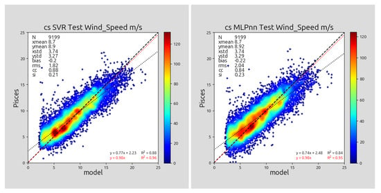
Figure 9. Above: Scatter plots for North Celtic Sea. Training cases for SVR; NN above, testing cases below.

Table 6. Statistics of multiple cell radar wind speeds compared to CERRA. Units (where relevant) are m/s.

Site		ML	N	x-mean/std	y-mean/std	bias	rms	cc	si
Liverpool Bay	TRAIN	SVR	9528	8.61/3.63	8.61/3.32	0.00	1.40	0.92	0.16
CERRA		NN			8.54/3.40	0.07	1.27	0.94	0.15
	TEST	SVR	9528	8.19/3.52	8.39/3.18	−0.20	1.76	0.87	0.21
		NN			8.26/3.27	−0.07	1.85	0.85	0.23
South Celtic Sea	TRAIN	SVR	9194	8.08/3.74	8.00/3.07	0.09	2.03	0.84	0.25
CERRA		NN			8.30/3.33	−0.21	1.69	0.89	0.21
	TEST	SVR	9194	8.35/3.18	7.53/2.48	0.81	2.53	0.67	0.29
		NN			7.87/2.77	0.47	2.68	0.62	0.32
North Celtic Sea	TRAIN	SVR	9199	9.34/3.69	9.33/3.38	0.01	1.33	0.93	0.14
CERRA		NN			9.42/3.66	−0.08	1.16	0.95	0.12
	TEST	SVR	9199	8.70/3.74	8.90/3.27	−0.20	1.82	0.88	0.21
		NN			8.98/3.54	−0.28	2.03	0.85	0.23

The SVR model can then be applied to all radar data for a particular time to obtain wind maps. Examples of these are shown in Figure 10 superimposed with model winds, satellite and in situ winds where available. The Liverpool Bay and the first South Celtic Sea maps use a mix of data used in the model development and data that were not used. The second South Celtic Sea map is created using no data involved in the development of the SVR model.

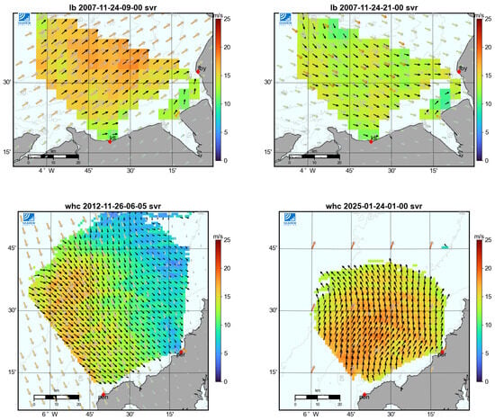
Figure 10. Wind maps for Liverpool Bay (above) and South Celtic Sea (below) using SVR using individual radar site ML models. Directions are shown with arrows: model data have a gray outline, satellite data are brown (when available), and in situ data are orange, each filled as per legend for higher wind speeds; radar is solid black; all arrow lengths are scaled by wind speed (colour-coded). Radar sites are indicated with ⧫. LB maps show speed and direction changes after 12 h. SCS maps: left wind field spatial variability for case where some locations were used in modeling, right south of Storm Eowyn. Note that the model winds on the Eowyn map are from ERA5 on a coarser grid.

3.2.2. Case 4: Combining All Radar Sites

ML SVR and NN models are obtained using training data from all three radar sites. The train and test wind speed statistics are shown in Table 7 and scatter plots in Figure 11. These models are then applied to individual sites and to all radar cells where there are corresponding wind model data, using all available radar data. These are compared with similar maps for the individual radar site cases. Figure 12, Figure 13 and Figure 14 show the statistics obtained with the individual cases above and the combined cases below. The top left map in each case shows the number of measurements included in the statistics. The positions of these cells are marked in black if they were used in the model development (so the model has "seen" half of the data at these points during training and testing), and blue for unused cells. The results are contoured using matplotlib’s tricontourf. These give a good indication of the performance of the ML models with reasonable agreement over most of the coverage, with some evidence of deterioration in performance at longer ranges and increased biases in the South Celtic Sea. The results obtained from the multi-radar multi-site models are largely similar to those for the single-radar multi-site models. Differences between the SVR and NN methods are small for all sites, with SVR having a slight edge in the wind speed statistics.

Table 7. Statistics for multiple cells, with multiple radar wind speeds compared to CERRA. Units (where relevant) are m/s.

Site		ML	N	x-mean/std	y-mean/std	bias	rms	cc	si
All Radars	TRAIN	SVR	19114	8.84/3.72	8.81/3.27	0.03	1.62	0.90	0.19
		NN			8.85/3.48	−0.01	1.61	0.90	0.18
CERRA	TEST	SVR	19120	8.45/3.15	8.41/3.05	0.04	2.00	0.83	0.24
		NN			8.43/3.33	0.02	2.11	0.81	0.25

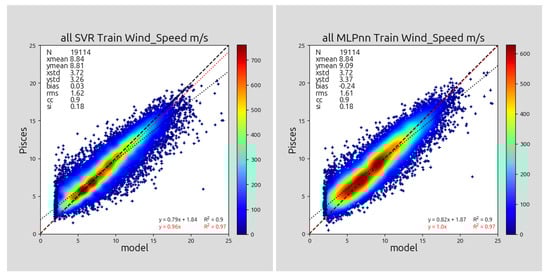
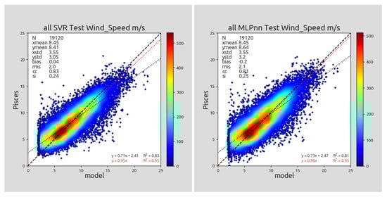
Figure 11. Above: Scatter plots using all radar sites. Training cases for SVR; NN above, testing cases below.

In this study, we used both vector correlation and phase (mean direction difference) defined by [22,23]. Ref. [11] recommended using the latter for wave accuracy assessment since the squared magnitude of the correlation is the proportion of variance (of the wind model data in our case) explained by a complex regression approach, so it is a direct analogue of the correlation coefficient for scalar variables. Both methods give similar results, so only the Hanson results are shown.

Figure 12. Wind accuracy maps for Liverpool Bay, using the following: left 2 columns—SVR, right—NN. Upper three row panels are the results when using model based on data from only Liverpool Bay; lower three row panels are the case when all sites were used to generate the model. The three rows show (1) the number of data samples (• are the train and test locations, • other co-location positions for validation) and wind speed bias; (2) wind speed rms and correlation; and (3) wind vector correlation, hvcorr, and phase, hphase, with the Hanson [23] method. Phases are cut off at ±15°, marked with a black line.

Figure 12. Wind accuracy maps for Liverpool Bay, using the following: left 2 columns—SVR, right—NN. Upper three row panels are the results when using model based on data from only Liverpool Bay; lower three row panels are the case when all sites were used to generate the model. The three rows show (1) the number of data samples (• are the train and test locations, • other co-location positions for validation) and wind speed bias; (2) wind speed rms and correlation; and (3) wind vector correlation, hvcorr, and phase, hphase, with the Hanson [23] method. Phases are cut off at ±15°, marked with a black line.

Figure 13. Wind accuracy maps for South Celtic Sea; details are the same as those shown in Figure 12.

Figure 13. Wind accuracy maps for South Celtic Sea; details are the same as those shown in Figure 12.

Figure 14. Wind accuracy maps for North Celtic Sea; details are the same as those shown in Figure 12.

Figure 14. Wind accuracy maps for North Celtic Sea; details are the same as those shown in Figure 12.

Figure 15 show maps at the same times as those in Figure 10. In three cases, the maps are similar, and this, together with the wind accuracy maps, suggests that a reasonable multi-site ML model has been found. However, the storm Eowyn winds are a little higher for the single-site case.

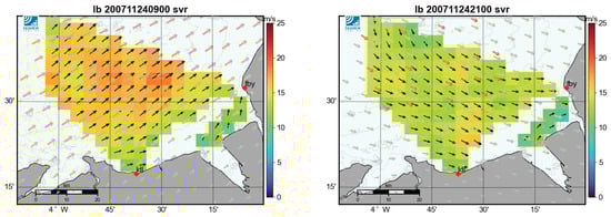
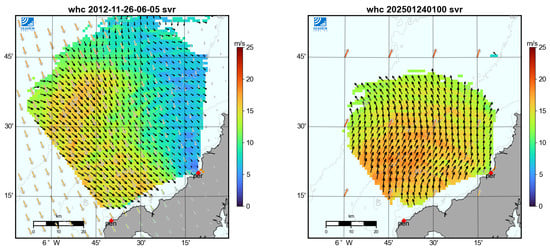
Figure 15. Wind maps for Liverpool Bay (above) South Celtic Sea (below) using SVR model obtained using data from all radar sites. Directions are shown with arrows: model data have a gray outline, satellite data are brown (when available), and in situ data are orange, each filled as per legend for higher wind speeds; radar is solid black; all arrow lengths are scaled by wind speed (colour-coded). Radar sites are indicated with ⧫. LB maps show speed and direction changes after 12 h. SCS maps: left Wind field spatial variability for case where some locations were used in modeling, right south of Storm Eowyn. Note that the model winds on the Eowyn map are from ERA5 on a coarser grid.

Further information about the performance of the ML models can be obtained using Taylor diagrams [24], as shown in Figure 16. Shown here are a number of different cases, either applied to all appropriate data for that case or to data from a particular radar cell. The cell chosen is near the centre of the coverage in each case. In a Taylor diagram, the best performance is achieved when the correlation coefficient (around the circumference) is near 1, the normalized rms difference (RMSD shown in green) approaches 0, and the normalized standard deviation is close to 1 (along the radii), so closest to 1 on the x-axis. For the case where all radars have been used to generate the model (noted as 3sites on the plot), the statistics have been applied to all the data and to the data where the CERRA wind speeds have been thresholded at 2, 5, and 7 $\mathrm{m}$/$\mathrm{s}$. A 10 $\mathrm{m}$/$\mathrm{s}$ threshold has also been used, but the amount of data is smaller, and the results are poorer. Note that the x- and y-axes are different, extending beyond 1 in some cases, but the SVR results look a little better than those of NN.

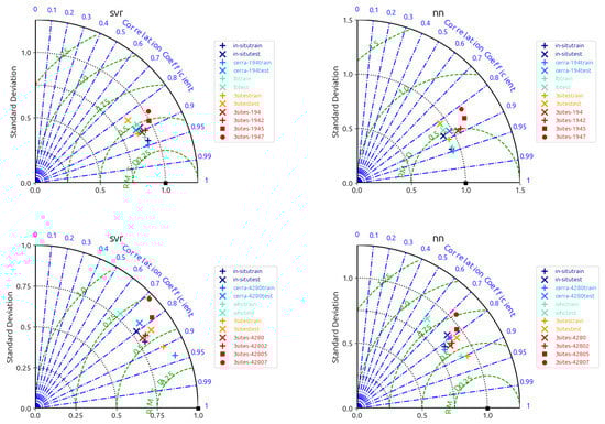
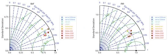
Figure 16. Taylor Diagrams for SVR model; NN on right. Top: Liverpool Bay, middle: South Celtic Sea. bottom: North Celtic Sea. Symbols refer to the different cases: in situ—ML model used data from local wind measurement (not available for cs) and nearest radar cell (dark blue); CERRA—data from CERRA and radar cell shown (light blue); sitename (lb, whc, cs)—CERRA and radar data at all selected cells for that site (cyan); 3 site—data from all radars and CERRA at all selected cells (orange), then applied to the specific radar cell shown (red lb: 194, whc: 4280 and cs: 220). In the latter case, the results include 2, 5, and 7 $\mathrm{m}$/$\mathrm{s}$ wind speed threshold cases (last integer in the label). The training cases are marked with +; the test cases are marked with x, with the exception of the red labels, which are all test cases.

Looking first at SVR training performance for the CERRA cases, for the lb and cs sites, the single-cell result is slightly better than the multi-cell, single-site one, which, in turn, is slightly better than the multi-cell, multi-site case. The latter is better than the multi-cell, single-site result for the whc site. The behavior is similar for the test cases, although at whc, the multi-cell, multi-site case is now the best. The test performances follow a similar pattern and, in all cases, are, as expected, not as good as the training cases. Applying a 2 $\mathrm{m}$/$\mathrm{s}$ threshold to the application of the multi-cell, multi-site at a single cell yields slightly better results across all sites. Higher thresholds decrease the correlation coefficient and increase the normalized rms but improve the normalized standard deviation.

Information on the wind vector performance using the Hanson metrics for some of the same cases is shown in Figure 17, using the same symbols (bold in this case for clarity) and colour-coding. Here, all the training and testing data have been used. There is very little difference between SVR and NN. In all three cases, the multi-cell, multi-site model applied at a single cell shows larger direction differences (hphase), with correlation increasing when higher thresholds are applied. The multi-cell, single-site results are different for the three sites from the other cases, with a higher correlation at cs and lower at lb. Nonetheless, all correlations are greater than 0.9, and direction differences are well within 5 degrees.

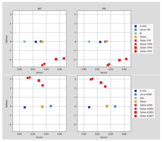
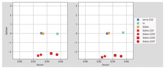
Figure 17. Hanson complex correlation, hvcorr, and direction difference (in degrees), hphase. Top: Liverpool Bay, middle: South Celtic Sea. bottom: North Celtic Sea. Labeling is the same as in Figure 16.

4. Discussion

The goal of this work was to develop a wind speed algorithm that can be applied across the field of view of an HF radar system and is significantly more accurate than our current method, which is used in our operational software, but we do not recommend it to customers. That method uses an inverse wind-wave model [25], which does not account for underdeveloped or decaying seas or significant swell. A clear illustration of the improvement that has been obtained is seen in Figure 18 and Table 8. Figure 18 uses all the data at the CERRA cells for all three radars, so for the ML case, it includes both training and testing data. The corresponding statistics for the new method applied only to the test data set are shown in the table for comparison. The scatter plot on the left extends to much higher (and incorrect) radar wind speeds, explaining the large rms value. Note that only limited quality control has been applied to the data sets used in this paper; normally, we limit our wind speed estimates to locations where wave data are obtainable [11]. This would have reduced the scatter for our old method, although nowhere near the reduction obtained with the SVR method, and also significantly reduced the spatial coverage (see final figure below). The ML wind speed estimates are clearly much more robust to noise. The comparison with the CERRA vs in situ data shows that the new radar results are similar, which is very encouraging.

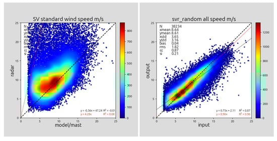
Figure 18. Comparison of existing Seaview wind measurement (left) accuracy relative to CERRA compared with the model developed in this paper using all radar sites and multiple cells (right) applied to the combined train and test data set from all sites and cells.

Table 8. Statistics of existing and new SVR radar wind speed estimates compared to CERRA. The testing-only statistics (from Table 7) and CERRA vs in situ statistics (from Table 3) are shown for comparison. Units (where relevant) are m/s.

Site	N	x-mean/std	y-mean/std	bias	rms	cc	si
OLD	38234	8.64/3.65	44.10/139	−35.45	143.88	0.00	16.13
NEW	38234		8.61/3.16	0.03	1.82	0.87	0.21
NEW test only	19120	8.45/3.55	8.41/3.05	0.04	2.00	0.83	0.24
LBmast				−0.29	1.50	0.92	0.20
M5buoy				−0.31	1.80	0.89	0.22

As seen in the accuracy maps (Figure 12, Figure 13 and Figure 14), most of the errors are confined to regions around the edge of the coverage, either at long range or large azimuth from one or both radars. This suggests that improvements could be made by better quality control of the radar data used in the algorithm development. Applying a wind speed threshold of 5 $\mathrm{m}$/$\mathrm{s}$ to the CERRA data before calculating statistics, as shown in Figure 19, does reduce the rms a little but increases the bias. The Taylor diagrams suggest that a 2 $\mathrm{m}$/$\mathrm{s}$ threshold may be better. There is very little difference in the directional statistics.

Figure 19. Wind accuracy maps with a 5 $\mathrm{m}$/$\mathrm{s}$ threshold for South Celtic Sea; details are the same as shown in Figure 12; for comparison with Figure 13.

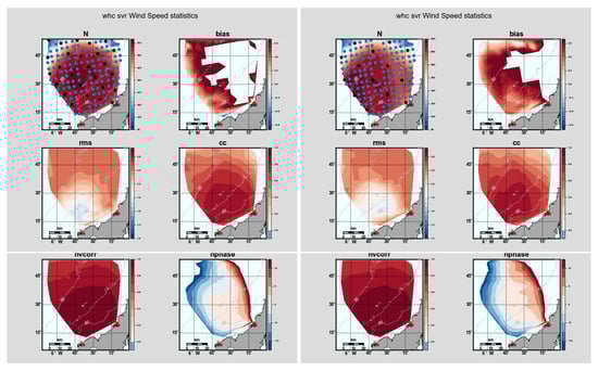
Figure 20, Figure 21 and Figure 22 show 3 days of hourly wind speed and direction maps and, where available, model and satellite wind vectors for qualitative validation. In general, the radar winds show more spatial variability than model or satellite data, but there is reasonable agreement between them. Over this period, there are 72 h of radar measured winds, 24 h of model and 3 of satellite data. The variation in space and time of the radar measurements looks realistic. Note that, as is the case for HF radar coverage for currents and waves, the spatial extent varies with time, being noticeably smaller in the high-wind period shown in Figure 22.

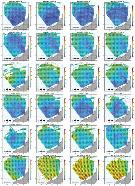
Figure 20. 24/11/2012 hourly wind maps; arrow notation is the same as shown in Figure 15.

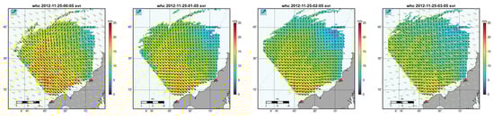
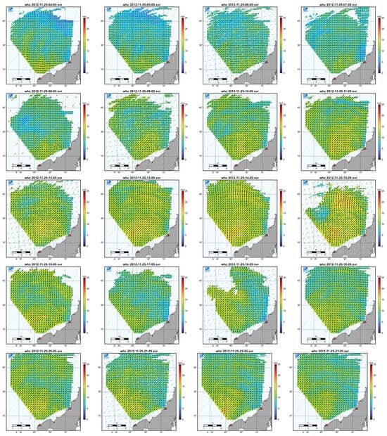
Figure 21. 25/11/2012 hourly wind maps; arrow notation is the same as shown in Figure 15.

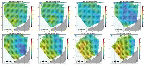
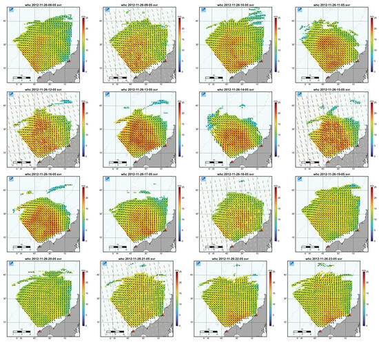
Figure 22. 26/11/2012 hourly wind maps; arrow notation is the same as shown in Figure 15.

Having established the reliability of the method, it needed to be implemented into the Seaview operational software package in order to provide near-real-time wind measurements. The model is stored in a netCDF file, which can now be used in the software to obtain wind speed measurements. The SVR wind speeds, therefore, appear in the inversion output file and can be downloaded, mapped, etc., using standard utilities. Figure 23 shows the original Seaview wind speed, using the standard Seaview mapping facility, for the Storm Eowyn case shown in Figure 15 and the map with the new wind speeds, which is very similar to the one in the earlier figure.

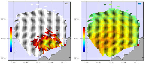
Figure 23. Storm Eowyn wind maps. Left: original Seaview wind speed colour-coded where white is greater than the maximum; right: SVR wind speed. Arrows show wind direction. • marks the radar location.

5. Conclusions

A machine learning method using support vector regression was developed in this study to provide significantly improved wind speeds from HF radar data than those previously available. Wind speed mapping with this method, using both data used in the development of the method and other data, has been demonstrated. The method makes use of CERRA wind model data as "sea-truth" and, where available, satellite data are used to qualitatively validate both radar and CERRA wind maps. A neural network method was also tested and gave similar but not quite as good results.

Recommendations for future work include the following:

1.

Explore better quality control of the radar parameters used in the ML modeling to reduce errors at longer ranges and examine the sensitivity of the model to these parameters and their uncertainties.

2.

Whilst a range of frequencies in the lower half of the HF range have been used in this work, the resulting model needs to be tested and perhaps modified to ensure the method can also be applied over the full HF range. Similarly, the amount of model data at high wind speeds was limited, so further training may be required in these circumstances.

3.

Although the ML model has been shown to provide reasonable wind speeds at all three of the sites in this paper, it would be useful to apply it to a wider range of geographical sites to firmly establish site independence.

4.

Using wind model data to train the ML model to obtain the radar wind speed measurements may introduce bias due to inadequacies/limitations in the wind model. More validations with offshore wind masts would be very useful to firmly establish the credibility and robustness of the radar wind measurements.

5.

Since the neural network results were similar to those obtained with SVR, it may be worth exploring alternative NN approaches, although, at the moment, it seems to be more complicated to implement these in the operational software. Explainability methods may be required to better understand how this approach works.

6.

The method presented here requires Doppler spectra from two radars—a dual configuration. Developing a solution for data from single radars would be useful.

References

- Roarty, H.; Cook, T.; Hazard, L.; George, D.; Harlan, J.; Cosoli, S.; Wyatt, L.; Fanjul, E.A.; Terrill, E.; Otero, M.; et al. The Global High Frequency Radar Network. Front. Mar. Sci. 2019, 6, 164. [Google Scholar] [CrossRef]
- Rubio, A.; Mader, J.; Corgnati, L.; Mantovani, C.; Griffa, A.; Novellino, A.; Quentin, C.; Wyatt, L.; Shulz-Stellenfleth, J.; Horstmann, J.; et al. HF Radar Activity in European Coastal Seas: Next Steps Toward a Pan-European HF Radar Network. Front. Mar. Sci. 2017, 4. [Google Scholar] [CrossRef]
- Fujii, S.; Heron, M.L.; Kim, K.; Lai, J.W.; Lee, S.H.; Wu, X.; Wu, X.; Wyatt, L.R.; Yang, W.C. An Overview of Developments and Applications of Oceanographic Radar Networks in Asia and Oceania Countries. Ocean Sci. J. 2013, 48, 69–97. [Google Scholar] [CrossRef]
- Wyatt, L.R. The IMOS Ocean Radar Facility, ACORN. In Coastal Ocean Observing Systems; Elsevier: Amsterdam, The Netherlands, 2015; pp. 143–158. [Google Scholar] [CrossRef]
- Wyatt, L.R. Ocean wave measurement. In Ocean Remote Sensing Technologies—High-Frequency, Marine and GNSS-Based Radar; Huang, W., Gill, E.W., Eds.; The Institution of Engineering and Technology: London, UK, 2021; pp. 145–178. [Google Scholar]
- Wyatt, L.R. Shortwave direction and spreading measured with HF radar. J. Atmos. Ocean Tech. 2012, 29, 286–299. [Google Scholar] [CrossRef]
- Emery, B.; Kirincich, A. HF radar observations of nearshore winds. In Ocean Remote Sensing Technologies—High-Frequency, Marine and GNSS-Based Radar; Huang, W., Gill, E.W., Eds.; The Institution of Engineering and Technology: London, UK, 2021; pp. 191–216. [Google Scholar]
- Wyatt, L.R. Progress towards an HF radar wind speed measurement method using machine learning. Remote Sens. 2022, 14, 2098. [Google Scholar] [CrossRef]
- Howarth, M.J.; Player, R.; Wolf, J.; Siddons, L.A. HF radar measurements in Liverpool Bay, Irish Sea. In Proceedings of the OCEANS 2007—Europe, Aberdeen, UK, 18–21 June 2007. [Google Scholar]
- Lopez, G.; Conley, D.C. Comparison of HF Radar Fields of Directional Wave Spectra Against In Situ Measurements at Multiple Locations. J. Mar. Sci. Eng. 2019, 7, 271. [Google Scholar] [CrossRef]
- Wyatt, L.R.; Green, J.J. Developments in scope and availability of HF radar wave measurements and robust evaluation of their accuracy. Remote Sens. 2023, 15, 5536. [Google Scholar] [CrossRef]
- Wyatt, L.R.; Green, J.J.; Middleditch, A.; Moorhead, M.D.; Howarth, J.; Holt, M.; Keogh, S. Operational wave, current and wind measurements with the Pisces HF radar. IEEE J. Oceanic Eng. 2006, 31, 819–834. [Google Scholar] [CrossRef]
- Gurgel, K.W.; Antonischki, G.; Essen, H.H.; Schlick, T. Wellen Radar (WERA): A new ground-wave HF radar for ocean remote sensing. Coast. Eng. 1999, 37, 219–234. [Google Scholar] [CrossRef]
- Shearman, E.D.R.; Moorhead, M.D. Pisces, a coastal ground-wave HF radar for current, wind and wave mapping out to 200 km ranges. In Proceedings of the IGARSS’88 Symposium, Edinburgh, UK, 12–16 September 1988; European Space Agency: Paris, France, 1989; pp. 773–776. [Google Scholar]
- Lipa, B.J.; Nyden, B.; Ulman, D.; Terrill, E. SeaSonde radial velocities: Derivation and internal consistency. IEEE J. Oceanic Eng. 2006, 31, 850–861. [Google Scholar] [CrossRef]
- Schimanke, S.; Ridal, M.; Le Moigne, P.; Berggren, L.; Undén, P.; Randriamampianina, R.; Andrea, U.; Bazile, E.; Bertelsen, A.; Brousseau, P.; et al. CERRA Sub-Daily Regional Reanalysis Data for Europe on Single Levels from 1984 to Present. Copernicus Climate Change Service (C3S) Climate Data Store (CDS). 2021. Available online: https://cds.climate.copernicus.eu/datasets/reanalysis-cerra-single-levels?tab=overview (accessed on 14 January 2025).
- Ridal, M.; Bazile, E.; Le Moigne, P.; Randriamampianina, R.; Schimanke, S.; Andrae, U.; Berggren, L.; Brousseau, P.; Dahlgren, P.; Edvinsson, L.; et al. CERRA, the Copernicus European Regional Reanalysis system. Q. J. R. Meteorol. Soc. 2024, 150, 3385–3411. [Google Scholar] [CrossRef]
- Patra, A.; Oueslati, B.; Chevallier, T.; Renaud, P.; Kervella, Y.; Dubus, L. Evaluation of ERA5, COSMO-REA6 and CERRA in simulating wind speed along the French coastline for wind energy applications. Adv. Sci. Res. 2025, 22, 69–85. [Google Scholar] [CrossRef]
- OSI SAF. ASCAT L2 25 km Winds Data Record Release 1—Metop, EUMETSAT SAF on Ocean and Sea Ice. 2016. Available online: https://user.eumetsat.int/catalogue/EO:EUM:DAT:METOP:OSI-150-A (accessed on 16 March 2026).
- Pedregosa, F.; Varoquaux, G.; Gramfort, A.; Michel, V.; Thirion, B.; Grisel, O.; Blondel, M.; Prettenhofer, P.; Weiss, R.; Dubourg, V.; et al. Scikit-learn: Machine Learning in Python. J. Mach. Learn. Res. 2011, 12, 2825–2830. [Google Scholar]
- Friedman, J.H. Greedy Function Approximation: A Gradient Boosting Machine; Technical Report; Stanford University: Stanford, CA, USA, 1999. [Google Scholar]
- Kundu, P.K. Ekman veering observed near the ocean bottom. J. Phys. Oceanogr. 1976, 6, 238–242. [Google Scholar] [CrossRef]
- Hanson, B.; Klink, K.; Matsura, K.; Robeson, S.M.; Willmott, C.J. Vector correlation: Review, exposition, and geographic application. Ann. Assoc. Am. Geogr. 1992, 82, 103–116. [Google Scholar] [CrossRef]
- Taylor, K.E. Summarizing multiple aspects of model performance in a single diagram. J. Geophys. Res. 2001, 7183–7192. [Google Scholar] [CrossRef]
- Dexter, P.E.; Theodorides, S. Surface wind speed extraction from HF sky-wave radar Doppler spectra. Radio Sci. 1982, 17, 643–652. [Google Scholar] [CrossRef]
Disclaimer/Publisher’s Note: The statements, opinions and data contained in all publications are solely those of the individual author(s) and contributor(s) and not of MDPI and/or the editor(s). MDPI and/or the editor(s) disclaim responsibility for any injury to people or property resulting from any ideas, methods, instructions or products referred to in the content. |
© 2026 by the authors. Licensee MDPI, Basel, Switzerland. This article is an open access article distributed under the terms and conditions of the Creative Commons Attribution (CC BY) license.