Highlights
What are the main findings?
- Despite significant algorithmic improvements and methodological shifts in automated deep learning models, they have not yet matched the precision of human interpreters.
- Analysis of the spatial distribution of studied glaciers reveals a strong regional bias in current data.
What are the implications of the main findings?
- The methodological shift allows for processing vast amounts of satellite data that would be unfeasible to handle manually, but the accuracy gap implies that human experts are still required for high-precision studies and to validate model outputs.
- The regional bias in current data implies a need to develop benchmarking datasets that include images from Arctic regions outside of Greenland and Svalbard to ensure model transferability and robustness.
Abstract
Calving front position is a key indicator of glacier and ice-sheet dynamics and an important variable for assessing mass loss and sea-level rise. Rapid growth in satellite data availability and image analysis techniques has driven the development of numerous automated calving front detection algorithms; however, the methodological landscape remains fragmented. This scoping review aims to map the existing literature on automated calving front detection, characterize the types of algorithms and data sources used, and identify trends, gaps, and challenges in current approaches. A systematic search of major bibliographic databases and complementary sources was conducted to identify studies describing automated or semi-automated calving front detection from satellite imagery or derived datasets. Eligible studies included peer-reviewed articles and relevant grey literature using optical, synthetic aperture radar (SAR), or multi-sensor data. Data were charted using a predefined framework that captures the algorithmic approach, input data characteristics, spatial and temporal coverage, validation strategies, and reported performance metrics. The review identifies a wide range of methods, from early threshold- and edge-based techniques to recent machine learning and deep learning approaches, with a strong shift toward convolutional neural networks over the past few years. Despite methodological progress, validation practices and evaluation metrics remain heterogeneous, and standardized benchmark datasets are scarce. This scoping review provides a structured overview of the field and highlights priorities for future methodological development and benchmarking.
1. Introduction
The calving front (CF) is defined as the boundary between the glacier tongue or ice shelf and the open ocean. CF marks the line where large chunks of ice break off to form icebergs in a process known as calving. This front plays a key role in the mass loss of marine-terminating glaciers [1] and ice sheets [2], indirectly contributing to the global rise of sea level. Monitoring changes in the position of the calving front is crucial for understanding glacier dynamics, as calving events are influenced by multiple factors, including ocean currents, water temperature, and internal stress within the ice sheet. CF variations are indicators of glacier health and can signal the acceleration of ice flow into the ocean through their retreat. Satellite imagery, including optical and synthetic aperture radar, is often used to map and monitor these fronts, providing critically important data for ice sheet models to predict future sea-level contributions [3].
Initially, field campaigns were the only way to measure the position of calving fronts. Such campaigns were logistically challenging, hazardous, and characterized by limited spatial and temporal coverage. Later, aerial photogrammetry was implemented to remotely acquire much more detailed information safely and quickly over a large area [4]. Subsequently, satellite data have begun to make their way into the field of CF detection, first as coast line line detection [5,6,7], then as antarctic coast line detection [8,9,10,11], and finally as CF detection cases [12,13,14].
Until the deep learning era, most studies of calving flux or ice-shelf modeling used manual delineations, which limited their spatial extent and temporal resolution. However, with the rise in satellite data availability, accelerated by the launch of Landsat 7 and Sentinel-1, manual identification of CFs became unfeasible. Attempts to automate CF detection based on satellite imagery date back to the 1990s [15,16] but were restricted by computing capabilities and processing techniques. Deep learning (DL) enabled automatic detection of CF in satellite imagery with reasonable accuracy that is systematically improved [17,18,19,20]. However, manual delineation is still more accurate [21] and is preferred in some studies [22,23].
Algorithms for automated CF detection have evolved drastically since the 1990’s, particularly in the last six years, and neural networks have emerged as the most widely used method. Despite significant progress in this area, as of 2018 [24], there has been no dedicated review of such algorithms. Among the achievements presented, some of the authors added sections focused on the current state of the art, but these sections were mostly limited to similar algorithms or areas of interest. The most comprehensive description was presented in [3]. The most recent comparison methods, including Vision Transformers and Foundation models, are described in [25]; however, it only analyzes the DL-based algorithms. Our review, in addition to the description of the algorithms, includes descriptions of viable benchmarking dataset options that expand on the work of [3] with newer, automatically generated datasets.
Here, we present a comprehensive overview of automatic methods for determining CF in satellite-derived data, developed since their first appearance in the field. By summarizing existing achievements in CF detection and the resulting benchmarking datasets, we hope to accelerate the improvement of DL models for CF detection.
2. Materials and Methods
2.1. Literature Search and Selection
The protocol for this review was created based on the Preferred Reporting Items for Systematic reviews and Meta-Analyses extension for Scoping Reviews (PRISMA-ScR) [26]. This research was preregistered on the Open Science Framework portal under the same title as the manuscript [27]. Our review combines the information from all peer-reviewed articles published until November 2025. We have considered all reports found in the the Crossref database through keyword queries. The initial search was conducted with a Crossref API, where ”glacier calving front“, ”glacier terminus“, and other phrases were searched for in titles, keywords, and abstracts. Results with a unique DOI identifier were then filtered to exclude all works regarding mountain glaciers. From the resulting pool, only works using satellite data were selected, and only those with any form of automation remained. After the initial search, we used a Research Rabbit AI tool [28] for further suggestions of articles, all carefully evaluated. The exact keyword sets and number of results are presented on the flow diagram in Figure 1. All remaining articles were carefully analyzed by two reviewers and charted based on the following variables:
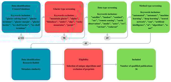
Figure 1.
Flow diagram presenting the process of literature search and filtering. Numbers in gray boxes represent the number of publications left after each filtering step.
- Number of glaciers studied;
- Names of glaciers studied;
- Satellite images which were used in the study;
- Type of satellite images used in the study;
- Number of processed satellite images;
- Dates of image acquisitions or, for larger datasets, a period in years;
- Type of algorithm tested (statistical, CNN, ViT, Foundation model);
- Brief description of an algorithm;
- Task design (zone or edge or simultaneous zone and edge segmentation or direct edge delineation);
- Evaluation metrics used in the study;
- Values of evaluation metrics;
- Publication of study results.
During the analysis of records, we identified publications related to the same core algorithm. In such cases, only the first implementation was described in detail, with other use cases mentioned afterwards.
Algorithms were assigned to groups according to type, and analyzed and described within each group. The values of the validation metrics were compared only if two algorithms were trained and tested on the same data, and the metrics were calculated in the same way (especially the mean distance error ()).
2.2. Validation Metrics
Different metrics are used to assess the accuracy of models depending on the type of product they return. The binary and zone segmentation are validated based on the correct classification of each pixel. Different metrics take into account the different ratios of True Positives (the model correctly predicts the positive class), True Negatives (the model correctly predicts the negative class), False Positives (the model incorrectly predicts positive class, e.g., ground truth marks the pixel as a background and model marks it as a calving front) and False Negatives (the model incorrectly predicts the negative class, e.g., ground truth marks the pixel as a calving front and model marks it as a background). The most commonly used metrics for binary classification are Intersection over Union ( or Jaccard score) [29] and the Dice coefficient (or -score) [30].
Both and have values ranging from zero (no overlap between prediction and label) to one (perfect overlap between prediction and label). Because and are derived from the same components of the confusion matrix, reporting both metrics is mathematically redundant.
In contrast to strict definitions and formulas used for and metrics, the mean distance error () was calculated differently between studies. The can be calculated as the mean distance between the pixels of the predicted CF and a label [3,18,31].
where I is the set of all evaluated images, P is the set of ground truth front pixels of one specific image, and Q is the set of corresponding predicted front pixels in that image.
For vectorized CF lines, a closely related metric, the Polygon and Line Similarity () metric [32], can be implemented as in [33].
The alternative approach to can be the calculation of the mean distance between the prediction and ground truth lines measured on equally spaced transects [34,35,36].
where T is the set of equally spaced transects along the predicted CF.
In case the distance between transects is equal to zero, the would take the form of Area over Front (A/F) [17,34,37].
where is an area between the ground truth and the predicted CF, and is the length of the predicted CF.
The and metrics are designed for comparing binary segmentation results. However, they are sometimes used for validating multiclass segmentation, where all but the tested class are treated as background. The results for each class are then averaged for comparability purposes. The metric is more sensitive to small misalignment and should not be used if the target class was the CF itself. The -score is less sensitive in the case of CF classification, but it is also not recommended to use it in heavily imbalanced cases. In terms of , differences in calculation methods limit the possibility of comparing studies to those that use the same formula.
3. Review Results
For our study, we identified 111 articles on CF research and subsequently filtered them by glacier type (mountain/tidewater), CF detection method (manual/automatic), and input data (satellite/in situ). Of these, 49 sources were assessed for eligibility. All preprints were discarded. Subsequent uses of the same model were considered for the dataset review or, if invalid, discarded. As a result, 36 publications were selected for the review. To facilitate comparison across sources, they are grouped by the core automation approach used.
3.1. Statistical Algorithms
The first study to tackle the automation of CF detection from satellite data is [14]. Sohn and Jezek started with a single ERS-1-derived SAR image of the Jakobshavn Glacier, from which they obtained texture information. The authors used local dynamic thresholding [38] on both the texture image and the denoised SAR image, which were combined to produce a binary image, which was later processed with Robert’s edge detection algorithm [39]. The final result was obtained using the recursive edge-tracing algorithm [15] and filtering edges by length. The same processing pipeline was later applied to individual images derived from aerial photography and from the Corona and SPOT satellites [40], demonstrating the model’s applicability to different image types. CF position snapshots from 1962, 1985, 1988, and 1992 formed a scattered time series. Sohn and Jezek added region-growing to filter results [16] and used modified processing on the same ERS-1 and SPOT scenes as in a previous study. The accuracy of the algorithm was assessed through visual comparison with the source imagery and was estimated to be within 2–3 image pixels, corresponding to ∼200 m on the ground. The upgraded version of the algorithm based on local adaptive thresholding was proposed a few years later by Liu and Jezek [10]. Modifications included extended image filtering, patch-based processing, threshold modeling based on a bimodal intensity distribution rather than texture, and aerial thresholding of the results. The algorithm proposed by Liu and Jezek [10] was applied to the Radarsat mosaic [41] to delineate a complete Antarctic coast. The results were compared with large-scale topographic maps [9] and manual delineations on SPOT panchromatic imagery using distance sampling at approximately 30–50 m, resulting in mean distances of 28.2 and 105.4 m, respectively. However, the algorithm required manual intervention, especially in the correction of the results.
Similarly to Liu and Jezek [10], Klinger et al. [42] proposed an algorithm to automatically delineate the Antarctic coastline in the image mosaic. However, Klinger et al. [42] decided to use the Landsat Image Mosaic of Antarctica (LIMA) [43] compiled from images from 1999–2003. The LIMA mosaic has a spatial resolution of 240 m. The authors noticed that land ice and ice shelves, sea ice, and rock outcrops differ significantly in the hue, saturation, and intensity parameters. These parameters were later used to identify the transition scenario for each segment of the Antarctic Digital Database (ADD) coastline [9]. The proposed algorithm is based on the active contour mechanism [6], which iteratively updates the initial contour placement based on internal energy (elasticity and rigidity) and external energy (Gradient Vector Flow [44] derived from input data). The authors compared the results with the manually delineated coast, which resulted in an RMSE value of 380 m. The main issue of the described model is the need for manual inspection of the selection of the transition scenario (6% of the segments) and manual correction of the results. Incorrect scenarios are selected if the initial contour is shifted by more than 2 km from the correct placement (erroneous georeferencing of SAR data during production of the ADD coastline). Post-processing is required due to the high number of false negative (∼12%) and false positive detections (∼14%).
Edge-enhancing algorithms such as Sobel [45], Canny [46], or Roberts [39] are frequently used in the detection of CF as a pre- or postprocessing mechanism, e.g., [10,16]. They are used as filters of fixed size and weight, or to highlight edges in a specific orientation [47]. Liu et al. [47] proposed the use of a 2-D wavelet transform instead of traditional edge operators. The derivative of a 2-D Gaussian smoothing function with scales ranging from 7 to 209 pixels is applied in the form of convolution to an input image. Points with the maximum value of the gradient modulus are connected using an algorithm from [48] to create maxima chains. In addition to length, these chains also carry information about their shape (open or closed), the average modulus value of all points in the chain, and the general orientation of the chain. Closed chains are immediately discarded. The maxima chains are then filtered separately on each spatial scale, and the remaining chains are aggregated. Of them, five with the highest score (based on length and scale-normalized average modulus value) are selected for time series filtering, where the advance/retreat rates calculated from these chains are compared with the average glacier flow velocity. Three iterations of time series filtering discard unrealistic results. The final chain is selected on the basis of the length-modulus score. The 2-D Wavelet Transform Modulus Maxima method was applied to ten terminating marine glaciers in Greenland based on Landsat 8 panchromatic imagery. The results were compared with manual delineations and yielded a value of 12.5 m for the median distance under clear imaging conditions. However, in the presence of sea ice, shadows, or thick cloud cover, the algorithm failed, underscoring its strong dependence on imaging conditions.
Profiling is a method of segmentation simplification in which 2-D data is sampled to a 1-D product. Seale et al. [49] proposed profiling-based processing and applied it to daily MODIS images of 32 Greenlandic Glaciers, spanning summers 2000–2009. The cropped and horizontally rotated images were processed with the Sobel edge filter. In parallel, intensity values in the image columns (across the glacier flow) are averaged, and the distribution of the average intensity is modeled to find the most likely position of the CF. The coherence between the Sobel-filtered pixels and the Gaussian curve peak, as well as between the Sobel-enhanced pixels and the CF position from previous delineations, is calculated to identify the point most likely to be a true CF position. The resulting position of CF was evaluated against the manual delineations presented in [50] with ∼190 m RMSE. The biggest drawback of this method is that the CF position is simplified to a single point. Han et al. [51] processed SAR images of the Upsala Glacier (Southern Patagonia Icefields, Argentina-Chile border) from 2007–2012. They sampled the images at equidistant intervals along the glacier borders. The moving window strategy is implemented to calculate the statistics that are later used to obtain the pixel scores. The five largest values, each from a different 1000-m segment of a profile, are kept for further filtering. The moving window of the cross-sectional profiles is used to find an area with the highest sum of pixel scores. Finally, for each profile, the points within the active area with the highest score are retained as CF points. Discretizations of the CF position were acceptable, especially in comparison to the single points produced by Seale et al. [49]. The average distance between the detected and true CF points was calculated for a single image and was 12.04 m. Another variation of the profiling method was implemented by Zhu et al. [52], where the authors implemented the Constant False Alarm Rate (CFAR) algorithm [53] as a pixel classifier. The presented CFAR method uses a sliding window mechanism with an exclusion buffer around the central pixel to gather the pixel intensities from both sides of the central pixel. Pixel intensities from both sides are summed separately. The lower of the two sums (the smallest of CFAR) is chosen to select all pixels with an intensity exceeding that sum. Selected pixels are used to model a threshold based on the Weibull distribution. The central pixel is then classified as an ice shelf (value of 1) if it exceeds the threshold or as a background (value of −1) otherwise. The classified image is processed with morphological dilation and erosion, and equidistant profiles are placed on the glacier ice shelf. The points in the profiles representing CF are selected as the maximum cumulative value along each profile. The authors tested their approach only on the Amery Ice Shelf. They used SAR imagery from each month in a period between March 2015 and May 2021, allowing them to analyze seasonal variations of the CF position with a mean distance error of 7.88–45.12 m.
The processing pipeline presented in [54] used Dijkstra’s shortest path search algorithm [55] to calculate the best CF line between two fixed points on both sides of Zachariae Isstrœm. CF is traced on the graph constructed from pixel centroids serving as nodes and connections to all neighboring pixels as edges. Each edge is weighted on the basis of the average endpoint values of the reversed edge-enhanced SAR image. The algorithm was tested on single images from the TerraSAR-X and Sentinel-1 satellites from 2016 and yielded values of 159 m and 246 m from manually delineated CFs, respectively. The second statistical algorithm of the same research group is described in [56]. The model uses height-sensitive terrain characteristics derived from digital elevation models (DEM). The algorithm starts by calculating the distribution of height values within a 60-pixel buffer around the baseline, which is the ADD coastline. Pixels with values lower than the 30th percentile are immediately classified as water/sea ice, and pixels with values higher than the 70th percentile are classified as land ice/ice shelf. These pixels serve as the seed points for the algorithm. Later, the unclassified pixels are processed in a spreading fire manner, starting from the pixels closest to the seed points. The unclassified pixels are labeled identically to the pixel with the smallest feature distance in its neighborhood. The feature distance is based on the height-sensitive terrain feature, which is calculated as the visual roughness of the DEM, averaged over the median interquantile range of values within a baseline buffer. Among all the approaches found, this study is the only one to detect CF based solely on DEMs, namely the TanDEM-X and the Reference Elevation Model of Antarctica (REMA) [57]. Experiments were conducted on the Fleming Glacier, glaciers in Mikkelsen Bay and Darbel Bay in the Antarctic Peninsula, and Zachariae Isstrœm in Greenland. For each site, DEMs from 2012, 2013, 2014, and 2017 were processed, yielding a mean (A/F) value of 56 m and an of 50 m compared to manual delineations.
The nine statistical models described in this section were based on global and local thresholding, active contours, profiling, edge detection and filtering, and game theory. The key information for each model, such as the regions, periods, and baselines studied, is summarized in Table A1 to allow for a clear comparison of the results between any two models.
In summary, statistical methods and conventional image processing techniques represented an important pioneering step in the automation of calving front detection. Their main advantage is that they are relatively computationally light and often do not require extensive, manually annotated training data sets. However, the analysis in Table A1 shows that their key weakness is their high sensitivity to variable weather conditions, cloud cover, and difficult environments such as the presence of ice melange. Furthermore, these algorithms often required manual intervention and complex pre-/post-processing, which prevented fully automated large-scale analysis and ultimately forced a paradigm shift towards machine learning.
3.2. Convolutional Neural Network-Based Algorithms
In 1991, a multilayer perceptron, a simple fully connected neural network (NN), was used to detect shorelines in aerial photography [7]. Almost 30 years later, U-Net [58] was utilized for the detection of CF in [59] and numerous subsequent studies. In this subsection, we will describe improvements to the U-Net to fine-tune it for CF detection, and introduce other CNN architectures well-suited for the task.
3.2.1. U-Net with Minor Modifications
The first to propose a U-Net-based algorithm for CF detection in satellite data were Mohajerani et al. [59]. Their semantic segmentation algorithm was trained and tested on Landsat 5–8 images of 4 Greenlandic glaciers, namely Helheim, Jakobshavn, Kangerlussuaq, and Sverdrup. Mohajerani et al. [59] decided to segment images into CF/non-CF classes, which poses a challenge due to the class imbalance problem. In such a scenario, the NN reaches high accuracy by simply classifying all pixels as non-CF. To mitigate this drawback, the authors scale the loss values for false negative classifications by the average ratio of non-CF to CF pixels in their training dataset. The authors decided to feed their U-Net with images of the whole CF, which were rotated so the glacier flow headed north, cropped out, and downsampled to fit the input size of 240 × 152 pixels. Mohajerani et al. [59] experimented with their algorithm, testing the influence of data augmentation, batch size, and U-Net depth on the results. They concluded that image flipping leads to more continuous lines and higher accuracy, label dilation leads to more continuous lines at the cost of accuracy, and a deeper NN does not introduce any improvements due to the small training dataset (123 images). Their final model (29 layers paired with data augmentation) yielded a mean distance to manually delineated CFs of 96 m.
Based on the work of Mohajerani et al. [59], Putatunda et al. [31] fused the attention mechanism [60] with the squeeze-excitation module to enhance critical features while suppressing background noise. The squeeze-excitation module consists of global average pooling (squeezing a feature map to a single value) followed by two dense layers with ReLU and sigmoid activation functions, respectively. The created channel-wise weights are used to scale the feature maps produced by the attention gate before combining them with the encoder features. The resultant network improved by more than 50%, lowering it to a value of 48.51 m, and achieved an -score of 73%.
The second to publish their achievements in the implementation of U-Net in CF detection was Baumhoer et al. [34]. The authors used 38 polarized SAR images stacked with a DEM on a 4-band input, modifying the U-Net accordingly. Furthermore, they enlarged the input tile size to 780 × 780 pixels at the cost of halving the number of feature channels. Baumhoer et al. [34] kept the more common methodology and segmented the images into ice/non-ice zones, in contrast to direct CF detection in [59]. The dataset used by Baumhoer et al. [34] was rather diverse, including images of 16 glaciers in Antarctica, but the temporal resolution of two months left room for improvement. Baumhoer et al. [34] evaluated their classification results against the ADD coastline in Marie Byrd Land in 2018 with recall, precision [61], and metrics for ice and water classes separately. Additionally, they calculated the from manually delineated CFs based on equidistant transects. The ice class was predicted with 90% precision, 93% recall, and 91% -score. The water class was predicted with 92% precision, 89% recall, and 90% -score. The calculated was equal to 154 m. The authors also mentioned that the A/F value is equal to 108 m.
The third basic implementation of U-Net was presented by Zhang et al. [20], who used a larger 5 × 5 convolutional kernel and 4 × 4 upsampling kernel, as well as the LeakyReLU activation function. Zhang et al. [20] compiled a dataset consisting of 159 images from TerraSAR-X of the Jakobshavn Glacier from the period between 2009 and 2015. The authors used the Greenland Ice Sheet Climate Change Initiative products as a baseline for their algorithms’ performance assessment, but first, they re-georeferenced satellite imagery and prepared their own labels manually. The A/F calculation between the manually obtained labels and the baseline yielded a mean distance of 104 m, largely due to georeferencing errors in the CCI product. The postgeoreferencing comparison between the network-predicted CFs and the CCI products yielded a mean distance error of 38 m.
The German Aerospace Center team continued to investigate the influence of input data on NN performance, initiated by Baumhoer et al. [34]. The resulting publication [35] focused on multispectral data. Loebel et al. [35] reconfigured the U-Net to accommodate up to 17 channel inputs, of which 10 are Landsat-8 bands, 6 are textural features extracted from the panchromatic band, and the last is the topography of the ocean bed [62]. The authors step-by-step eliminated an input feature to establish its influence on CF detection at 23 Greenlandic and 2 Antarctic glaciers. The dataset consisted of 997 multispectral Landsat images taken between 2013 and 2021. The authors compared their results with manually delineated CFs, using mean and median distances (30 m spaced transects) and binary classification metrics such as -score. Loebel et al. [35] found that only the addition of multispectral data improved the model’s median distance performance compared to single-band panchromatic input. The mean distance improved in all cases except for the combination of multispectral data and textural data. The model trained on all available features produced the best results across all metrics, except median distance, which was lowest when using only multispectral data. In general, the fully equipped model produced a mean distance of 44.9 m, a median distance of 28.6 m, a binary classification accuracy of 99.1%, and an -score of 99.31%. In the following years, Loebel et al. tested their network on spatially extended datasets, but restricted to nine multispectral bands [2,63].
Similarly, as Loebel et al. [35] expanded the work of Baumhoer et al. [34], another team used the U-Net proposed by Zhang et al. [20] to prepare a series of articles [3,64,65,66,67,68] on its further modifications and applications. In their first paper, Davari et al. [64] test the Matthews correlation coefficient (MCC) [69] as an early training stopping metric and propose the creation of distance map-based labels and the loss function (distance map-based binary cross-entropy) [70]. Both methods are proposed as mechanisms to mitigate the problem of class imbalance. The model was trained and tested on a multimission SAR dataset consisting of 244 images of Sjogren Inlet and DBE Glacier (Antarctica) and 169 images of Jakobshavn Glacier (Greenland). The MCC tests included both zone and edge segmentation, whereas the loss-function tests used only edge segmentation. The results were compared with manual delineations based on , , and MCC. The metrics included three levels of tolerance for edge segmentation cases. The final model, including both modifications and with ∼100 m tolerance, produced an of 40.72%, a of 55.06%, and an MCC of 55.66% for glaciers of the Antarctic Peninsula, and an of 67.14%, a of 80.10%, and an MCC of 79.57% for the Jakobshavn Glacier.
Further expanding the work of Davari et al. [64], Holzmann et al. [65] kept the DBCE loss function, tested the -score as an early stopping mechanism, and added the attention gates [60] to the U-Net’s skip connections. The attention mechanism merges the inputs from skip connections (features) with outputs from a one-step-deeper upscaling path (gating signal) and, through a series of convolutional and activation layers, produces an attention map, which is pixel-wise multiplied by all features from the skip connections. Experiments with baseline U-Net and Attention U-Net were performed using different loss functions (BCE, DBCE with distance weights of 4, 8, and 16) and compared with manual delineations of the Sjogren Inlet and DBE Glacier. The dataset used in this study was a subset of [64] with an image count of 244 and a time span of 1995–2014. Attention, U-Net outperformed the baseline U-Net only with the DBCE loss function with distance weight equal to 8 (Dice of 70.8% and of 56.1%). However, the baseline U-Net (with the standard BCE loss function and without the attention gates) produced the highest overall of 73.9% and of 60.6%.
Subsequent work by Hartmann et al. [66] was dedicated to the assessment of uncertainty in the output of the U-Net and its incorporation as a focus mechanism for a second U-Net. Again, the basis for this experiment is a U-Net proposed by Zhang et al. [20]; however, in this case, dropout layers with a relatively high rate of 50% are applied after each block, except the last. The modified network is called Bayesian U-Net after [71]. Each input is processed 20 times, which, paired with a random dropout of weights in each block, acts as a Monte Carlo simulation framework. The pixel-wise variance of errors is calculated to produce the uncertainty map, which is then binarized by a threshold of 0.125 and stacked with a raw image, creating a 2-band input for a second identical Bayesian U-Net. However, this time, the results were averaged to produce the final segmentation output. Hartmann et al. [66] used exactly the same dataset as in Holzmann et al. [65], but their algorithm performed zone segmentation rather than edge segmentation. Therefore, the resultant and values were significantly higher and equal to 95.24% and 90.91%, respectively. However, compared with the unmodified U-Net of Zhang et al. [20], the improvements were statistically insignificant (0.38% improvement with a standard deviation of 6.57% for and 0.69% improvement with a standard deviation of 3.40% for ).
Davari et al. [67] built on the achievements of their previous papers to reformulate U-Net processing as a pixel-wise regression task and incorporate it into CF detection. It was done by transforming the training labels into distance maps, as in [64], and using the mean squared error (MSE) as a loss function. In particular, this is the only case of a NN used in a pixel-wise regression framework for CF detection. The authors experimented with postprocessing algorithms, namely global thresholding, Conditional Random Field (CRF) [72], and a second U-Net (without the modifications mentioned above), of which the latter yielded the best results. Again, the authors used the dataset from [65], expanded with SAR images from the Jorum, Crane, and Mapple Glaciers, increasing the image count to 418. The evaluation protocol included a few tolerance levels, and the algorithm proposed at each level achieved approximately a two-fold improvement. With a tolerance of 100 m, the pixel-wise regression U-Net followed by the edge segmentation U-Net produced results with an -score of 46.29% and an of 30.63%, while the baseline U-Net achieved values of 12.33% and 6.99% of the respective metrics.
Periyasamy et al. [68] summarized previously presented work and fine-tuned each processing step, including data preprocessing, data augmentation, loss function selection, bottleneck mechanism selection, normalization, and dropout ratio selection. The authors tested which of the proposed elements would result in the largest improvement in . In addition to the -score, the authors also reported scores in and accuracy. They concluded that additional filtering and histogram equalization improve the -score by 4.10%. Data augmentation, including image flipping and rotation, yielded the largest -score improvement of 7.30%. The selection of the equally weighted combination of BCE and the Dice loss function accounted for another 0.90% increase in . Dilated convolutions (with a dilation rate of 4), both alone and in combination with residual connections, performed almost identically in , increasing terms by another 2.61%. However, results obtained with combined dilated convolutions and residual connections yielded fewer false positives and false negatives than those obtained with only dilated convolutions. The last two elements, namely normalization and dropout optimization, did not improve the metric, and in the case of dropout, it even lowered the metric value at a dropout rate of 10%. Finally, an optimized U-Net was trained in a new area with weights transferred from previous experiments. Training was performed with some weights frozen (encoder or decoder), or with none frozen, and the results were compared with a fully retrained network. Freezing the encoder allowed for computational gains with minimal loss in accuracy. All model variations were trained and tested on a slightly reduced dataset from [64] with a SAR image count of 393. The optimized zone segmentation U-Net achieved an of 93.78%, an of 88.70%, and a precision of 97.40%.
Unlike in the five preceding papers, Gourmelon et al. [3] decided to use the original U-Net as proposed in [58], but with the inclusion of Atrous Spatial Pyramidal Pooling (ASPP) [72] in the bottleneck part of the architecture, and the loss function of Davari et al. [64] in edge segmentation and from Periyasamy et al. [68] in zone segmentation. ASPP is a set of parallel convolutional layers with different dilation rates ranging from 1 (standard convolution) to 8. Even though the authors proposed their own model trained individually for zone and edge segmentation, the main focus of this study is on the dataset that is prepared for benchmarking between different algorithms. The dataset consists of 681 multimission SAR images of 7 glaciers (Sjogren Inlet, DBE, Crane, Mapple, and Jorum Glaciers from Antarctica; Jakobshavn Glacier from Greenland; and Columbia Glacier from Alaska, USA) spanning the period from 1995 to 2020. The dataset is an extension of the dataset used in [64,65,66,67,68]. The proposed models are also meant for comparison purposes. Therefore, the models were comprehensively evaluated against manual delineations using recall, precision, -score, and for zone segmentation, and for edge segmentation. The scores obtained were as follows: precision of 84.2%, recall of 79.6%, -score of 80.1%, of 69.7%, and of 887 m. It is worth mentioning that the authors also reported binary classification metrics for edge segmentation and for zone segmentation. Clearly, the binary metrics for edge segmentation were significantly worse than those for zone segmentation. However, the obtained with zone segmentation was lower than that with edge segmentation and was 753 m. All results, labels, images, and codes used in this study were made available as open source in the form of a benchmark dataset, also presented in another article [73]. In a separate paper, Gourmelon et al. [74] tested the same model but replaced the postprocessing with a 2-D Conditional Random Field (CRF), with only a marginal improvement.
The CaFFe dataset was used again in [75], where the authors utilize the non-new U-Net framework (nnU-Net) in conjunction with a nine-step deep U-Net. The nnU-Net assumes that some of the hyperparameters required in NN training are insignificant, some are rule-based, and some are fixed based on the operator’s experience. The framework speeds up the process of hyperparameter tuning by reducing the possible combinations and values for each parameter. Additionally, Herrmann et al. [75] implemented multi-task learning (MTL), in which a network is branched to produce zone and edge segmentation, and benefits from enhanced feedback during training. Finally, they experimented with model training with the additional task of delineating the whole glacier boundary and with a fused label (edge pixels as an additional class for zone segmentation). All experiments, except for the standard single-task learning (STL) cases, achieved significantly better results than the baseline U-Net from [3]; however, the differences between the MTL experiments were not significant. The best performing model, the one with a boundary side task, achieved the of 509 m, the -score of 71.7 ± 0.5%, and the of 72.6 ± 0.4%, but due to the statistically insignificant difference in precision, the authors recommend the use of the model trained on fused labels.
3.2.2. U-Net with Major Modifications
Previously described studies utilized the U-Net with only slight adjustments. As a major modification, we introduced drastic changes to the U-Net architecture [37] and the coupling of the U-Net backbone with itself or other algorithms [18,19].
Song et al. [37] utilized the U-Net architecture, but instead of traditional encoder and decoder blocks, it included nested U-Net-like building blocks called Residual U-blocks (RSU). The RSU contains convolutional and downsampling layers, skip connections, and, in deeper parts of the network, dilated convolutions. In each RSU, the number of filters is kept unchanged despite the inclusion of pooling layers. This architecture is called U2-Net [76]. The U2-Net was trained on 20 Landsat panchromatic images of the Pine Island Glacier sampled twice a year in the period between 2013 and 2022. The study proved that U2-Net is able to learn to classify images into zones even with such a small dataset. However, the multiplication of parameter count due to nested RSU construction would likely prevent the model training on lower-end machines. The model was benchmarked with the Fully Convolutional Network (FCN) and the original U-Net, both of which struggled to learn to classify image patches with a single class. U2-Net achieved precision of 99.43%, recall of 99.54%, and of 94.04%. Although the model was tested on unseen data from Totten and Filshner Ice Shelves, it still lacks evaluation in a more diverse dataset.
Heidler et al. [18] focused on creating an algorithm that would be competitive in both zone and edge segmentation, without the need for separate training. The authors first identified the most significant parts of both image segmentation (encoder-decoder architecture) and edge segmentation algorithms (cross-resolution prediction merging) and combined them into a single model. Furthermore, they implemented a single loss function (adaptively balancing binary cross-entropy) that is robust to class imbalance and well-suited to both segmentation and edge detection tasks [77]. The resulting model combines a U-Net with 2 task-specific prediction heads, which merge predictions and weight maps from each decoder block into a single prediction. This architecture also enabled the authors to implement the deep supervision mechanism, which directly transferred additional loss values to each decoder block. The model was trained and tested on a dataset similar to that of Baumhoer et al. [34], but limited to glaciers in two regions, namely the Antarctic Peninsula and Wilkes Land (East Antarctica). The dataset used in this study consists of 16 SAR images that spanned June 2017 to December 2018. The model was compared with several statistical models and deep learning models, achieving the best results in all cases. The HED-UNet achieved accuracy, , and mean distance values of 80.5%, 67.2% and 345 m in the Antarctic Peninsula, and 92.0%, 84.9% and 222 m in Wilkes Land, respectively. HED-UNet was later trained on dual-polarization Sentinel-1 data and used in the production of a benchmark dataset called IceLines [78].
The work presented by Wu et al. [19] builds on the research described by Gourmelon et al. [3]. The proposed algorithm consists of 2 U-Nets, whose decoders are connected via 3 attention hooking gates. One branch, called the target branch, processes the center-cropped portion of the input image at full resolution. The second branch, called the context branch, processes the full input image downsampled to match the target image size. Attention hooking gates pass the center-cropped feature maps from context decoder blocks to the next-step target decoder blocks, matching the spatial coverage of both branches. The output of the attention gate is deeply supervised with the loss function that sums up the target, context, and deep loss components. An evolution of the research conducted by Gourmelon et al. [3], AMD-HookNet was trained and tested on the same dataset (CaFFe [73]), and evaluated with the same metrics as in [3], that is, precision, recall, -score, , and , achieving values of 85.0%, 85.0%, 84.3%, 74.4% and 438 m, respectively.
Some studies described in this review adapt the multi-task learning procedure [17,18,75], however, in all the cases mentioned, the output consists of zones and edges, whereas in [79] the secondary output is a semantic change map. The created U-ConvNextV2 mimics the U-Net encoder-decoder with skip connections architecture, at the same time incorporating the two-branch scheme, similar to [19]. The encoder of U-ConvNextV2 consists of ConvNextV2 blocks, which are inspired by the Swin-Transformer patch extraction. ConvNextV2 blocks downsample feature maps not by max pooling, which is a standard approach for most U-Net-based algorithms, but rather through depth-wise convolutions with large 7 × 7 kernels. Additionally, the Global Response Normalization (GRN) is used in each block to ensure consistency on different scales. The second branch of U-ConvNextV2 takes any other input image of the same size and, through the shared encoder and simplified decoder, extracts change information. The additional change-detection label is automatically generated from the zone segmentation labels prepared for the input images. The U-ConvNextV2 model was tested in the CaFFe dataset along with the baseline U-Net [3], HED-UNet [18], AMD-HookNet [19], and its successor, AMD-HookFormer [80]. The U-ConvNextV2 outperformed all the mentioned models achieving the -score of 71.5 ± 1.3%, of 59.0 ± 1.4% and of 398 ± 43 m.
When analyzing the group of algorithms based on the U-Net architecture, it should be emphasized that they have become the standard in glacier segmentation tasks due to their ability to effectively combine low- and high-resolution features. As shown in Table A2, their main strength is high precision in overall zone segmentation and relative simplicity of implementation. However, the greatest challenges remain problems related to extreme class imbalance (in the case of front segmentation), difficulties in accurately capturing edges without using additional complex architectural modifications or appropriate label preparation (fused labels), and the need for large, diversified, and labeled datasets to enable proper generalization.
3.2.3. Other Neural Networks
The first and, to our knowledge, the only implementation of VGG16 [81] in CF detection was presented by Marochov et al. [82], where it was paired with compact CNN (cCCN) [83]. The first processing stage involves training on Sentinel-2 RGB+NIR image tiles composed of >95% of single-class pixels and returns the class for the entire tile. The second stage utilizes the VGG16 product by processing it with a Multilayer Perceptron (MLP) to produce a pixel-level classification. The authors experimented with adding the NIR band, varying the input VGG16 tile size, and varying the convolutional layers preceding the MLP. The best results were achieved for 50 × 50 px input tiles, RGB+NIR four band input, and 15 × 15 px second-stage tiling followed by seven convolutional layers and an MLP. The final model returned the -score value of 92.2%. For fine-tuning, the authors added two images from each test site to the training dataset, which, as expected, resulted in a significant improvement in the -score on the unseen dataset, raising the overall -score to 97.5%.
The second NN architecture other than U-Net implemented in CF detection is DeepLabV3+ [72]. It was first implemented by Cheng et al. [17], which incorporates the Xception-65 NN as the backbone and the ASPP as a bottleneck. The model called CALFIN is trained on a diverse dataset, consisting of Landsat 1–8 images of 66 Greenlandic glaciers, as well as some SAR images of Antarctic glaciers. The authors used additional tiling of the 255 × 255 px input dividing it into nine 224 × 224 px tiles, which were processed separately to offer multiple independent classifications and lower the uncertainty of the results. The model produces both zone and edge segmentation simultaneously. The two-way output is used to filter the front segmentation output based on the deviation of the zone segmentation values. The images are processed twice, first with a buffer around the CF and later with a zoomed-in view of the CF. After postprocessing that included the longest path search in the image graph and the minimum spanning tree (MST) [84], the results were compared with manual delineation and the work of Mohajerani et al. [59], Baumhoer et al. [34], and Zhang et al. [20], in their respective datasets. The CALFIN model achieved a mean distance from manually delineated labels of 86.76 m and an of 97.93% (for zone output). In the Mohajerani and Zhang datasets, the CALFIN model closely matched the performance of the benchmark models, achieving mean distances of 97.72 m and 115.24 m, respectively. However, in a Baumhoer dataset, consisting exclusively of SAR data, CALFIN strongly deviated from the baseline, producing a mean distance three times that of the benchmark model.
In Zhang et al. [36] the authors used the same DeepLabV3+ NN as in Cheng et al. [17]. However, they experimented with different backbones, namely ResNet-101 [85], DRN [86], and MobileNet [87] architectures. In addition, Zhang et al. [36] settled on the zone segmentation rather than the combined output. The dataset used in this study was also different from that of Cheng et al. [17] by consisting of the majority of SAR data from the Jakobshavn, Kangerlussuaq, and Helheim Glaciers. Unique to this study was filtering the results based on their complexity, calculated from direction change frequency, polygon length, and the polygon and its convex hull areas. The best-performing model was DRN-DeepLabV3+ paired with histogram normalization in the preprocessing, with the A/F value of 86 ± 59 m. This model was used in later work to prepare a benchmark dataset called AutoTerm [88].
The last DeepLabV3+ implementation was performed by Heidler et al. [89] and in an extended version with more diverse benchmarking in [33]. The authors used the modified model of Cheng et al. [17], but removed the final activation layer, which was supposed to produce the final segmentation results. Instead, Heidler et al. [33] fed the prepared feature maps to the prediction head in the form of a 1D CNN. The prediction head, dubbed the snake head, was inspired by Peng et al. [90] and the active contour algorithm of Kass et al. [91]. The 1D input is produced by sampling the feature maps in initial vertex positions. The snake head is equipped with dilated 1D convolutional layers and performs predictions by adding the original vertex coordinates to the modeled vector. The authors stated that four passes are enough to produce meaningful results. The authors also implemented the loss function based on dynamic time warping [92], which first searches for the best alignment between two sequences, and then calculates pairwise distances. The loss function was also modified after [93], where the minimum operator was replaced by the soft minimum. For model training and testing, Heidler et al. [33] combined three publicly available datasets, namely Cheng et al. [17], Loebel et al. [35], and Baumhoer et al. [34]. Apart from using previously established datasets, the authors also tested numerous other models, both CNN and active contour-based. Furthermore, the authors used the special metric designed for polygon and polyline comparisons called [32]. Moreover, Heidler et al. [33] adapted the Monte Carlo Dropout methodology described by Gal and Ghahramani [71], and later improved by Hartmann et al. [66], to quantify their model uncertainty. The final model achieved the metric value of 99 ± 10 m, 144 ± 21 m, and 99 ± 12 m when tested in the CALFIN [17], Loebel [35], and Baumhoer [34] datasets, respectively. The COBRA model, as the authors dubbed it, was later used to process SAR images of the Svalbard archipelago [94,95].
The evolution towards other convolutional architectures shows an attempt to directly address the limitations of U-Net-based models. Their greatest strength, identified in Table A2, is their significantly better performance in directly extracting the glacier front line itself and the precise extraction of specific edge features. Nevertheless, these models come at a cost of more computational complexity, more difficult to optimize training, and can cause problems with generalization to new, previously unseen data without proper fine-tuning.
3.3. Vision Transformers
Transformers are mostly recognized as the algorithms behind the Large Language Models (LLMs); however, they can also be used in computer vision tasks (Vision Transformers or ViTs), as in [96]. Instead of convolutions, transformers divide an image into small patches and, via the self-attention mechanism, learn the important features. The patches are then merged, and the self-attention mechanism is used again. Iterations of self-attention and patch merging are repeated until the patches reach the input size.
The first case of CF detection with an algorithm that incorporates ViTs was GLA-STDeepLab [97]. Zhu et al. [97] modified the DeepLabV3+ model, replacing the convolutional and downsampling layers with Swin-Tansformers. The only convolutional layers remaining are dilated convolutions in the ASPP bottleneck layers. Each Swin-Transformer Block groups patches in 4 × 4 patch windows and calculates self-attention only within these windows. In subsequent odd transformer layers within the same Swin-Transformer Block, the windows are shifted to allow the information exchange between previously divided patches. In addition, the standard self-attention is modified by the addition of global-local attention, which constructs two parallel branches to extract the global and local contexts later combined with the self-attention outputs. The GLA-STDeepLab was trained and tested on the CaFFe dataset [73], achieving an -score of 97.07%, an of 94.35%, and an of 602 ± 76 m.
The first to implement the full ViT-based model in CF detection were Wu et al. [80], who rebuilt the AMD-HookNet architecture [19] and implemented Swin-Unet [98] instead of a U-Net. Swin-Unet is a U-shaped encoder-decoder architecture in which the convolutions are replaced by Swin Transformer Layers. As in the original U-Net, the Swin-Unet incorporates the skip connections between the encoder and the decoder. Wu et al. [80] initialized their model with ImageNet weights and fine-tuned the Contextual HookFormer on the CaFFe dataset [73]. The HookFormer model acquired a precision value of 85.9 ± 0.3%, a recall of 85.5 ± 0.4%, an -score of 84.8 ± 0.3%, an of 75.5 ± 0.3%, and an of 353 ± 16 m.
The second work describing the implementation of ViT in CF detection was [21], in which the authors paired the SwinV2 transformer [99] as an encoder with a Residual Convolutional Neural Network (RCNN) [85] as a decoder, and called the resulting model TYRION. The SwinV2 transformer differs from the previous version in the placement of normalization layers, the use of scaled cosine attention, and the treatment of inputs. The TYRION model is initialized with ImageNet weights, trained on a custom unlabeled dataset called SSL4SAR, and fine-tuned on the CaFFe dataset [73]. The SSL4SAR dataset consists of 9562 Sentinel-1 SAR images of 14 Arctic glaciers from 2015–2022. Additionally, for each glacier, the single, cloud-free, multispectral image from Sentinel-2 is resampled to the SAR image resolution. In pretraining, Gourmelon et al. [21] experimented with two multimodal training techniques, namely SSL4SAR-OptSimMIM and SSL4SAR-OptTranslator. The first method masks some of the SAR input patches and, via a single linear prediction head, predicts the pixel values in the optical image corresponding to these masked patches. The second method uses the single-layer convolutional prediction head to translate the SAR image into a multispectral optical counterpart. The authors evaluated the TYRION model based on on the CaFFe [73] labels. The best performing variation was the one pretrained with the OptTranslator method, with an of 293 ± 54 m across the entire CaFFe test set. Additionally, to comprehensively compare the AI model with the human annotator, Gourmelon et al. [21] prepared five individually retrained models, whose results were averaged for assessment and used to estimate classification uncertainty. The best-performing model in the multi-annotator study was TYRION-OptTranslator, achieving an of 75 m. However, human annotators achieved the 38 m , and the TYRION-OptTranslator model was able to surpass humans only in PALSAR image classification.
A foundation model is a large-scale machine learning model trained on a broad and diverse dataset. These models can be adapted to a wide range of downstream tasks with a little (few-shot) to no (zero-shot) fine-tuning. Foundation models are mainly based on ViTs because of their better performance on large datasets. We found only one case of the application of the foundation model in the detection of CF [100]. Shankar et al. [100] used the ViT-Large variant of the Segment Anything Model (SAM) created by Meta AI [101]. The author’s goal was to demonstrate SAM’s capability across a variety of glaciological tasks, namely crevasse, iceberg, supraglacial lake, and glacier terminus detection. In the CF segmentation, the authors used a single Sentinel-2 image. SAM performed exactly the same with and without additional information called prompts, achieving an -score of 96%. However, in crevasse segmentation, promptless prediction did not highlight any crevasse. It should be noted that prompt preparation and mask selection were performed manually by the authors. Additionally, SAM2, depending on the prompts, can try to segment either the glacier outlines or the entire coast, which may cause differences in accuracy and requires different postprocessing to retrieve the CF itself.
Although we found only three ViT-based algorithms, we placed them in a separate section due to their different processing approach. Notably, only one model, namely HookFormer, was built entirely of transformers, and the other two models included some parts based on convolutional layers. As the foundation models are also based on transformers, the ViT-based models are grouped together with them in the same summary Table A3. The fundamental advantage of ViTs over CNNs is their ability to model the global context of an image and capture long-range dependencies between pixels, which is extremely beneficial when analyzing large and complex fronts. However, the barriers to their widespread use are the enormous computational costs and the extremely high demand for training data.
Although the algorithms discussed in previous sections differ significantly in their technological approach, they all rely heavily on the specific characteristics of the geographic locations used for training and validation. To evaluate the representativeness of these datasets and identify potential regional biases in current research, we analyzed the spatial distribution of the areas studied. Figure 2 visualizes the spatial extent of glaciers examined in all relevant sources reviewed in Section 3.1, Section 3.2 and Section 3.3. The map explicitly includes glaciers identified by name or unique ID in the primary texts or supplementary materials attached to the analyzed publications. However, to maintain a focus on methodological development, the visualization excludes glaciers processed solely in subsequent applications or re-implementations of these algorithms, such as [63,78,94]. The central map shows the cumulative count of glaciers studied within different regions. In this metric, repeated processing of the same glacier in separate publications is counted individually, thereby highlighting the general research interest in a region rather than just the number of unique physical objects. The specific locations are detailed in the side panels, which mark the centroids (red dots) of all glaciers processed by the described algorithms.
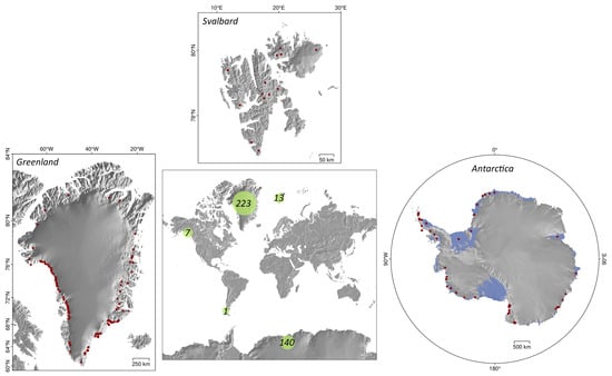
Figure 2.
Distribution of all glaciers studied across all found relevant sources. In the center, the numbers in green circles represent the cumulative count of studied glaciers, grouped by region. The above, right, and left panels present three main regions, with red dots representing centroids of all glaciers processed by the described algorithms.
3.4. Datasets
The majority of articles, especially those published after 2020, include some form of results publication. The authors primarily share the prediction results; however, some also include labels, input images, and the full code to allow reproduction and validation of the results. In Table A4, we compile the information about the datasets built for and processed by the algorithms described in this manuscript. For presentation purposes, we excluded the links that lead to each dataset or the code repository, as they are listed in the article describing each dataset. We ignored some of the datasets due to broken links [102] or presenting the CF position as a scalar value [47,103,104,105]. In addition to datasets containing automatically detected CF positions, datasets with manually delineated CF positions are also worth mentioning, as they can serve as high quality labels for future studies. Some of the most comprehensive datasets obtained manually are [23,106,107].
We found three datasets that offer data ready for use in benchmarking [35,63,73]. These datasets include images and labels used in model training, processing results, and codes for ease of reproduction of results. Of these three datasets, the CaFFe dataset [73] was the most received by the community and served as a benchmark for the models not only by the authors of the dataset themselves [19,21,75,80], but also by other researchers [79,97].
As most of the datasets focus on Antarctica and Greenland, it is especially worth noting that in 2024, the comprehensive dataset of CF positions in the Svalbard archipelago was published by [94]. Additionally, in 2025, the large unlabeled SAR-based dataset [21] was presented, covering 13 glaciers in Svalbard and one glacier in Alaska (USA). The unlabeled dataset is useless for supervised learning in CNN training, but it serves as a pretraining dataset for self-supervised learning, where the algorithm learns by reconstructing patches cropped from the image. Another interesting project is the IceLines dataset [78], which is automatically updated monthly. The IceLines dataset uses the HED-UNet algorithm [18], combined with an automated download and screening process, to fully automate the production of CF positions for 20 Antarctic glaciers.
Similarly to the previous section, we created a Figure 3 representing a map of all glaciers covered in the described datasets, to help identify the gaps in spatial coverage of the datasets. The center map shows the cumulative count of covered glaciers in different regions, and the side panels present centroids of all glaciers covered in three main regions, marked with red dots.
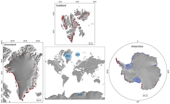
Figure 3.
Distribution of all glaciers covered across all found datasets. In the center, the numbers in blue circles represent the cumulative count of covered glaciers, grouped by region. The above, right, and left panels present three main regions, with red dots representing centroids of all glaciers covered in the datasets.
4. Discussion
Based on the map showing the spatial distribution of the results of the described algorithms, as well as the map showing the available CF products from automated processing, it is evident that the researchers’ focus is on Greenland and Antarctica. Only one of the algorithms presented was originally trained on data from the Svalbard Archipelago [21], and only one algorithm was retrained and used to delineate a large number of CFs in the said region [94]. Only two glaciers outside of Antarctica, Greenland, or the Svalbard region were analyzed in any of the described studies: the Upsala Glacier, the Southern Patagonia Ice Fields, and the Columbia Glacier in Alaska (USA). Columbia Glacier was included in the CaFFe dataset as a new region for testing purposes and shows the applicability of models to new study sites. The Svalbard datasets were recently presented in 2024 [94] and 2025 [21]. Therefore, we will likely see the presentation of other datasets covering the rest of the Arctic, including the Russian Arctic, Northern Canada, and Alaska.
Proper comparison of models can be performed only when the compared models were trained and tested on the same input dataset, the same metrics were used to quantify the results, and the metrics were calculated against the same baseline. In Table 1, we combine all studies that meet these requirements with three exceptions. Two of these examples refer to comparisons with Baumhoer et al. [34] and Mohajerani et al. [59] datasets, where subsequent studies used manual delineations as a baseline, but did not mention whether these delineations were preexisting or self-prepared. In the third case, Heidler et al. [33] compare their model with those of Baumhoer et al. [34] and Loebel et al. [35], however, as the authors of said benchmarks used the prepared for pixelated CF evaluation (4), Heidler et al. [33] use the vector-specific version (5) due to their prediction characteristics. These two metrics are similar and use a common methodology, but their formulas and input types (raster or polyline) differ. Therefore, the results of calculations based on pixel distances and the metric cannot be directly compared.

Table 1.
Overview of the validation metric values in comparable cases. The asterisk marks the model, which was not originally trained and tested on the common dataset. The value of validation metrics for [18] was calculated for benchmarking purposes in [79].
Comparable examples meeting all the requirements (common dataset, baseline, metrics) exist only for five datasets. The most widely used is the CaFFe dataset [73], particularly due to its ease of use. Gourmelon et al. [73] shared all the necessary data, including different labels for zones and edges, preprocessed SAR images divided into training and test parts, as well as baseline results and source code. Comparison of model performance on CaFFe dataset is presented in the Figure 4. All algorithms using the CaFFe dataset significantly improved compared to baseline U-Net [3], which is not the case in terms of and , where [18,79] performed worse than baseline. However, the segmentation metrics in [79] were calculated for only two of the four classes and only within the 1 km buffer around the detected CF. Consequently, the baseline metrics were lower, settling at 66.2 ± 1.2 and 52.5 ± 1.4 for and , respectively. In these conditions, both algorithms outperformed the baseline, as the validation metrics for HED-UNet on the CaFFe test set were reported in [79] rather than in the original article [18]. The difference in performance of the baseline model between the original and restricted cases suggests that it is focused on stable regions, such as rock outcrops, rather than the dynamically changing ice-ocean border. In general, the lowest in the CaFFe dataset was achieved by the TYRION-OptTranslator [21], however, the SSL4SAR dataset used in the pretraining contains images of the Columbia glacier, which is left out for testing in the CaFFe dataset. The inclusion of Columbia glacier images in pretraining might have skewed the results. The next-best-performing model was HookFormer [80] with an of 353 ± 16 m.
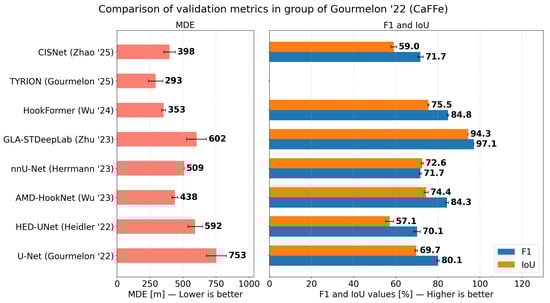
Figure 4.
Model validation metrics [18,19,21,75,79,80,97] compared to Gourmelon et al. [3] baseline. Left panel includes the values and the right panel includes and values.
Before the publication of the CaFFe dataset [73], parts of it were used in the second set of comparable studies [64,65,66,67,68], which results are charted in Figure 5. These five studies are based on the manual delineations of Seehaus et al. [108,109]. In addition, in each of these five studies, different numbers of glaciers (two to five) were used. The lowest count of two glaciers was used in [66], where the highest and scores were achieved, suggesting overfitting of the model. Moreover, the scores achieved by the baseline U-Net [20] are within the standard deviation of the results of [66], therefore, the improvement was insignificant.
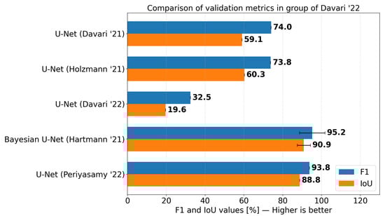
Figure 5.
Model validation metrics [64,65,66,67,68] compared to Davari et al. [64] baseline. Blue bars represent the -score and orange bars represent the values.
The other three comparison cases are conducted on the first three studies on the implementation of U-Net for the detection of CF [20,34,59]. Results of these studies are comapred in Figure 6. The authors of [20] noted the inconsistency of geocoding between the TSX images and optical images analyzed in Google Earth Engine (GEE). Zhang et al. [20] applied their own regeoreferencing based on ground control points to minimize error. These corrected images were not shared by the authors. Therefore, the high values of subsequent studies might be caused not only by the model itself but also by the input image georeferencing quality.
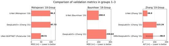
Figure 6.
Comparison of models validation metrics [17,20,31,36] grouped by the baseline—Mohajerani et al. [59] in the left panel, Baumhoer et al. [34] in the central panel, and Zhang et al. [20] in the right panel.
Although the TYRION-OptTranslator was the best performing model in terms of the value on the CaFFe dataset [73], humans outperformed it in the multi-annotator experiment [21]. Each retrained model and each human expert were evaluated against the manually obtained mean line. The model achieved an of 75 m, while humans achieved an of 38 m, proving that automated processing came closer than ever to human-level accuracy in CF detection.
Although automated calving front (CF) detection has seen significant improvements, a fundamental methodological dichotomy remains between zone segmentation and edge segmentation approaches. As highlighted by the variability in model performance, defining the task strictly as semantic zone segmentation [34,82]) often reduces the problem to delineating the general boundary of the glacier. In this approach, the model primarily learns global differences between the glacier and its surroundings, treating the CF merely as a byproduct of the boundary between the two zones. Consequently, such models may not capture the unique and highly localized physical characteristics of the calving front itself, such as the presence of crevasses, ice melange, and localized calving activity. By contrast, edge segmentation methods [59,89], or hybrid architectures [17,18] directly target the CF line, preventing the boundary interpretation from blurring with regular lateral margins or coastlines. However, it often suffers from an extreme class imbalance problem that has to be mitigated. One interesting approach to fusing zone segmentation and front segmentation is that of Herrmann et al. [75]. Apart from the standard classes introduced in the CaFFe dataset [73], Hermann et al. added a five-pixel-wide CF class at the boundary between the glacier and water classes. Even though the results were only as precise as those of other multitask learning experiments in the paper, the fused-labels approach reduces the number of parameters and shortens training time. Therefore, to narrow the accuracy gap between human interpreters and automated systems while maintaining computational efficiency, future research should increasingly explore fused label approaches. By explicitly incorporating the calving front as a distinct class alongside traditional zone masks, models can effectively target the specific structural features of the CF without the computational overhead of complex multi-branch architectures.
The review demonstrates that relying on standard semantic segmentation often falls short due to the extreme class imbalance in direct CF detection. Design choices that consistently improve performance involve explicitly addressing this imbalance. Successful strategies include implementing specialized loss functions, such as distance map-based binary cross-entropy [64], and adopting hybrid architectures. MTL approaches that simultaneously perform zone and edge segmentation [18,19], and models utilizing fused labels [75] consistently outperform baseline models by forcing the network to focus on the unique structural features of the CF rather than just the global glacier boundary.
While optical satellite data provide high-resolution multispectral features, their temporal generalization is fundamentally limited by cloud cover and polar nights. A partial solution to this limitation is the usage of the Harmonized Landsat Sentinel-2 (HLS) product, which combines data from both missions, shortening the revisit cycle and increasing the likelihood of cloud-free images. In contrast, SAR data generalize better across varying weather and illumination conditions, making them essential for continuous, year-round time series monitoring. The most promising recent advancement is multi-modal integration, such as the SSL4SAR dataset and OptTranslator models [21], which successfully leverage cloud-free optical imagery to guide and enhance feature extraction from SAR data during the pretraining phase.
5. Conclusions
This scoping review highlights a fundamental shift in automated calving front detection from statistical methods to Deep Learning architectures. While CNNs, particularly U-Nets, remain the current standard, the emergence of Vision Transformers marks a significant technological step. Our analysis confirms that these data-driven approaches outperform traditional techniques in handling complex textures in both SAR and optical imagery.
Despite these advancements, the field suffers from methodological fragmentation. The lack of standardized validation protocols, inconsistent baselines, and varying metrics (MDEs) makes direct comparison between studies challenging. Furthermore, there is a significant spatial bias, with research disproportionately focused on Greenland, Antarctica, and Svalbard, leaving other regions of the Arctic underrepresented.
To advance the field, the community must prioritize unified benchmarks and standardized datasets, such as CaFFe. Future research should focus on improving model accuracy to achieve human-level precision, generalizing the model for ice-sheet-wide applications, exploiting multimodal data fusion to mitigate sensor limitations, and leveraging self-supervised learning to reduce manual labeling costs. These steps are essential for developing robust operational systems capable of monitoring glacier dynamics globally.
Author Contributions
Conceptualization, M.S.; data curation, M.S. and M.T.; funding acquisition, W.M.; investigation, M.S.; methodology, M.S.; project administration, W.M.; visualization, M.S. and A.K.; writing—original draft preparation, M.S.; writing—review and editing, M.T., A.K. and W.M. All authors have read and agreed to the published version of the manuscript.
Funding
This research was funded by Wrocław University of Science and Technology within the Academia Professorum Iuniorum programme.
Data Availability Statement
No new data were created or analyzed in this study. Data sharing is not applicable to this article.
Acknowledgments
During the preparation of this manuscript/study, the authors used Writefull for the purposes of grammar correction. The authors have reviewed and edited the output and take full responsibility for the content of this publication.
Conflicts of Interest
The authors declare no conflicts of interest.
Appendix A
Table A1.
Summary of key information about studies utilizing statistical methods in CF detection.
Table A1.
Summary of key information about studies utilizing statistical methods in CF detection.
| Study | Region | No. of Studied Glaciers | Input Data | No. of Processed Images | Studied Period | Algorithm | Strengths | Weaknesses | Baseline |
|---|---|---|---|---|---|---|---|---|---|
| [15,16,40] | Greenland | 1 | Optical and SAR | 4 | 1962–1992 | Local dynamic thresholding | Simplicity | Sensitivity to imaging conditions | raw images |
| [10] | Antarctic | - | SAR | - | 09–10.1997 | Local dynamic thresholding | Simplicity | Manual intervention required | ADD (topographic maps) and manual delineations |
| [49] | Greenland | 32 | Optical | 105,536 | 2000–2009 | Profile method | High temporal resolution | Reduction of a CF to a single point | [50] |
| [42] | Antarctic | - | Optical | - | 1999–2003 | Active contours | Active contours implementation | Possible large errors due to poor initialization | [41] |
| [51] | Argentina | 1 | SAR | - | 2007–2012 | Profile method | Extensive results filtering | Discretization of the resulting line | manual delineations |
| [54] | Greenland | 1 | SAR | 2 | 2016 | Dijkstra’s shortest path | Simplicity | Dependence on the preprocessing method | manual delineations |
| [47] | Greenland | 10 | Optical | 460 | 2013–2020 | 2-D Wavelet Transform Modulus Maxima | Edge detection in multiple spatial scales | Sensitivity to imaging conditions | manual delineations |
| [52] | Antarctic | 1 | SAR | 75 | 2015–2021 | Constant False Alarm Rate and Profile method | Statistical semantic segmentation | Discretization of the resulting line | manual delineations |
| [56] | Greenland, Antarctic | 4 | Optical and SAR | - | 2012–2014, 2017 | Game theory | Fully DEM-based feature highlighting | Low temporal resolution of open-source DEMs | manual delineations |
Table A2.
Summary of CNN-based models for calving front detection. The comparison includes study regions, data sources, architectural approaches, and a subjective assessment of the strengths and weaknesses of each method.
Table A2.
Summary of CNN-based models for calving front detection. The comparison includes study regions, data sources, architectural approaches, and a subjective assessment of the strengths and weaknesses of each method.
| Study | Region | No. of Studied Glaciers | Input Data | No. of Processed Images | Studied Period | Algorithm | Strengths | Weaknesses | Labels | Compared with |
|---|---|---|---|---|---|---|---|---|---|---|
| [34] | Antarctic | 16 | SAR | 38 | 2018 | U-Net | Polarized SAR usage | - | Manual delineations | - |
| [59] | Greenland | 4 | Optical | 123 | 1985–2016 | U-Net | - | Resolution degradation in preprocessing | Manual delineations | - |
| [20] | Greenland | 1 | SAR | 159 | 2009–2015 | U-Net | - | Low spatial diversity of the dataset | Manual delineations | - |
| [17] | Greenland, Antarctic | 66 | Optical and SAR | 5153 | 1972–2019 | DeepLabV3+ | Comprehensive dataset | Accuracy at best equal to benchmark | Manual delineations | [20,34,59] |
| [64] | Greenland, Antarctic | 3 | SAR | 413 | not mentioned | U-Net | Class imbalance mitigation | Network fine-tuned for a specific region without the unseen data testing | manual delineations from [108,109] | [20] |
| [82] | Greenland | 3 | Optical | 40 | 2019–2020 | VGG16 | Implementation of multispectral data | Inclusion of a small portion of test images in training data | Manual delineations | Metric values presented in [17,20,34,59] |
| [65] | Antarctic | 2 | SAR | 244 | 1995–2014 | U-Net | Introduction of attention mechanism | Marginal improvement compared to baseline U-Net | manual delineations from [108,109] | [20] |
| [36] | Greenland | 3 | Optical and SAR | 2087 | 2002–2019 | DeepLabV3+ | Assessment of backbone influence on the results | Usage of glacier specific thresholds in results filtering | Manual delineations | [20] |
| [66] | Antarctic | 2 | SAR | 244 | 1995–2014 | U-Net | Estimation of results uncertainty | Not tested on the unseen data | manual delineations from [108,109] | [20] |
| [67] | Antarctic | 5 | SAR | 418 | 1995–2014 | U-Net | Unique pixel-wise regression | Processing causes loss of distance information | manual delineations from [108,109] | [20] |
| [3] | Greenland, Antarctic, Alaska (USA) | 7 | SAR | 681 | 1995–2020 | U-Net | Trained and tested on the benchmark dataset as a baseline for future studies | Low accuracy for a benchmark model | Manual delineations | - |
| [18] | Antarctic | 7 | SAR | 16 | 2017–2018 | U-Net | Simultaneous prediction of both zones and edges, extensively benchmarked | - | Manual delineations | Algorithms not described in this review |
| [35] | Greenland, Antarctic | 25 | Optical | not mentioned | 2013–2021 | U-Net | Implementation of multispectral data | - | Manual delineations | - |
| [68] | Greenland, Antarctic | 3 | SAR | 393 | 1995–2014 | U-Net | Fine-tuned | Low spatial diversity of the dataset | manual delineations from [108,109] | - |
| [19] | Greenland, Antarctic, Alaska (USA) | 7 | SAR | 681 | 1995–2020 | U-Net | Trained and tested on the benchmark dataset | - | Manual delineations from [73] | [3] |
| [33] | Greenland, Antarctic | 82 | Optical and SAR | 1997 | 1992–2021 | Active contours, DeepLabV3+ | High generalizing capability | Correct results only for images with a single CF | Manual delineations from [17] | [17,34,35] |
| [37] | Antarctic | 3 | Optical | 20 | 2013–2022 | U2-Net | Increased performance without the need for extensive dataset | High complexity and parameter count | Manual delineations | Metric values presented in [18,34,36,59] |
| [75] | Greenland, Antarctic, Alaska (USA) | 7 | SAR | 681 | 1995–2020 | U-Net | Extended statistical analysis of results | - | Manual delineations from [73] | [3] |
| [31] | Greenland | 4 | Optical | 123 | 1985–2016 | U-Net | Significant improvement over a benchmark model | Resolution degradation in preprocessing | Manual delineations from [59] | [3,36,59,65,80] |
| [79] | Greenland, Antarctic, Alaska (USA) | 7 | SAR | 681 | 1995–2020 | U-Net | Transformer-like downsampling | - | Manual delineations from [73] | [3,18,19,80] |
Table A3.
Summary of ViT-based models for calving front detection. The comparison includes study regions, data sources, architectural approaches, and a subjective assessment of the strengths and weaknesses of each method.
Table A3.
Summary of ViT-based models for calving front detection. The comparison includes study regions, data sources, architectural approaches, and a subjective assessment of the strengths and weaknesses of each method.
| Study | Region | No. of Studied Glaciers | Input Data | No. of Processed Images | Studied Period | Algorithm | Strengths | Weaknesses | Labels | Compared with |
|---|---|---|---|---|---|---|---|---|---|---|
| [34] | Antarctic | 16 | SAR | 38 | 2018 | U-Net | Polarized SAR usage | - | Manual delineations | - |
| [59] | Greenland | 4 | Optical | 123 | 1985–2016 | U-Net | - | Resolution degradation in preprocessing | Manual delineations | - |
| [20] | Greenland | 1 | SAR | 159 | 2009–2015 | U-Net | - | Low spatial diversity of the dataset | Manual delineations | - |
| [17] | Greenland, Antarctic | 66 | Optical and SAR | 5153 | 1972–2019 | DeepLabV3+ | Comprehensive dataset | Accuracy at best equal to benchmark | Manual delineations | [20,34,59] |
| [64] | Greenland, Antarctic | 3 | SAR | 413 | not mentioned | U-Net | Class imbalance mitigation | Network fine-tuned for a specific region without the unseen data testing | manual delineations from [108,109] | [20] |
| [82] | Greenland | 3 | Optical | 40 | 2019–2020 | VGG16 | Implementation of multispectral data | Inclusion of a small portion of test images in training data | Manual delineations | Metric values presented in [17,20,34,59] |
| [65] | Antarctic | 2 | SAR | 244 | 1995–2014 | U-Net | Introduction of attention mechanism | Marginal improvement compared to baseline U-Net | manual delineations from [108,109] | [20] |
| [36] | Greenland | 3 | Optical and SAR | 2087 | 2002–2019 | DeepLabV3+ | Assessment of backbone influence on the results | Usage of glacier specific thresholds in results filtering | Manual delineations | [20] |
| [66] | Antarctic | 2 | SAR | 244 | 1995–2014 | U-Net | Estimation of results uncertainty | Not tested on the unseen data | manual delineations from [108,109] | [20] |
| [67] | Antarctic | 5 | SAR | 418 | 1995–2014 | U-Net | Unique pixel-wise regression | Processing causes loss of distance information | manual delineations from [108,109] | [20] |
| [3] | Greenland, Antarctic, Alaska (USA) | 7 | SAR | 681 | 1995–2020 | U-Net | Trained and tested on the benchmark dataset as a baseline for future studies | Low accuracy for a benchmark model | Manual delineations | - |
| [18] | Antarctic | 7 | SAR | 16 | 2017–2018 | U-Net | Simultaneous prediction of both zones and edges, extensively benchmarked | - | Manual delineations | Algorithms not described in this review |
| [35] | Greenland, Antarctic | 25 | Optical | not mentioned | 2013–2021 | U-Net | Implementation of multispectral data | - | Manual delineations | - |
| [68] | Greenland, Antarctic | 3 | SAR | 393 | 1995–2014 | U-Net | Fine-tuned | Low spatial diversity of the dataset | manual delineations from [108,109] | - |
| [19] | Greenland, Antarctic, Alaska (USA) | 7 | SAR | 681 | 1995–2020 | U-Net | Trained and tested on the benchmark dataset | - | Manual delineations from [73] | [3] |
| [33] | Greenland, Antarctic | 82 | Optical and SAR | 1997 | 1992–2021 | Active contours, DeepLabV3+ | High generalizing capability | Correct results only for images with a single CF | Manual delineations from [17] | [17,34,35] |
| [37] | Antarctic | 3 | Optical | 20 | 2013–2022 | U2-Net | Increased performance without the need for extensive dataset | High complexity and parameter count | Manual delineations | Metric values presented in [18,34,36,59] |
| [75] | Greenland, Antarctic, Alaska (USA) | 7 | SAR | 681 | 1995–2020 | U-Net | Extended statistical analysis of results | - | Manual delineations from [73] | [3] |
| [31] | Greenland | 4 | Optical | 123 | 1985–2016 | U-Net | Significant improvement over a benchmark model | Resolution degradation in preprocessing | Manual delineations from [59] | [3,36,59,65,80] |
| [79] | Greenland, Antarctic, Alaska (USA) | 7 | SAR | 681 | 1995–2020 | U-Net | Transformer-like downsampling | - | Manual delineations from [73] | [3,18,19,80] |
Table A4.
Datasets containing viable CF positions for use in future studies.
Table A4.
Datasets containing viable CF positions for use in future studies.
| Paper | Labels | Images | Data Type | No. of Images | Period Covered | No. of Glaciers | Region | Algorithm | Strengths | Weaknesses |
|---|---|---|---|---|---|---|---|---|---|---|
| [20] | yes | no | SAR | 159 | 2009–2015 | 1 | Greenland | U-Net | - | Only Jakobshavn glacier |
| [17] | no | yes, as an image ID | optical | 5153 | 1972–2019 | 66 | Greenland | DeepLabV3+ | Long observational record | Only CF predictions |
| [36] | yes | yes, as an image ID | Optical and SAR | 2087 | 2002–2019 | 3 | Greenland | DRN-DeepLabv3+ | Integration of datasets with different spatial resolutions | Glacier specific criterion for results filtering |
| [35] | yes | yes | optical | 995 | 2013–2021 | 25 | Antarctic Peninsula, Greenland | U-Net | Multispectral data | - |
| [73] | yes | yes | SAR | 681 | 1995–2020 | 7 | Antarctic Peninsula, Greenland, Alaska (USA) | U-Net | Dedicated benchmark dataset with zones and front labels | Compiled with only SAR data |
| [78] | no | yes, as an image ID | SAR | ongoing | 2014– | 20 | Antarctic | HED-UNet | Regularly updated | - |
| [88] | from [106] | yes, as an image ID | Optical and SAR | 430,000 | 1984–2021 | 295 | Greenland | DRN-DeepLabv3+ | Full pipeline with data download, preprocessing and uncertainty estimation | - |
| [63] | yes | yes | optical | 1220 | 2013–2021 | 23 | Greenland | U-Net | Multispectral data | - |
| [94] | no | yes, as an image ID | Optical and SAR | 1,135,074 | 1985–2023 | 149 | Svalbard | Active contours, DeepLabV3+ | High temporal resolution, multi-sensor data | - |
| [2] | yes | yes, as an image ID | optical | 1220 | 2013–2023 | 47 | Antarctic Peninsula | U-Net | Multispectral data | - |
| [21] | no | yes | Optical and SAR | 9576 | 1995–2022 | 14 | Svalbard, Alaska (USA) | SwinV2-Transformer | Large unlabeled dataset | Useful only in transformer pretraining |
References
- Tielidze, L.G.; Mackintosh, A.N.; Yang, W. Glacier inventories reveal an acceleration of Heard Island glacier loss over recent decades. Cryosphere 2025, 19, 2677–2694. [Google Scholar] [CrossRef]
- Loebel, E.; Baumhoer, C.A.; Dietz, A.; Scheinert, M.; Horwath, M. Calving front positions for 42 key glaciers of the Antarctic Peninsula Ice Sheet: A sub-seasonal record from 2013 to 2023 based on deep-learning application to Landsat multi-spectral imagery. Earth Syst. Sci. Data 2025, 17, 65–78. [Google Scholar] [CrossRef]
- Gourmelon, N.; Seehaus, T.; Braun, M.; Maier, A.; Christlein, V. Calving fronts and where to find them: A benchmark dataset and methodology for automatic glacier calving front extraction from synthetic aperture radar imagery. Earth Syst. Sci. Data 2022, 14, 4287–4313. [Google Scholar] [CrossRef]
- Carbonnell, M.; Bauer, A. Exploitation des Couvertures Photographiques Aériennes: Répétées du Front des Glaciers Vêlant dans Disko Bugt et Umanak Fjord, Juin-Juillet 1964; C.A. Reitzel: København, Denmark, 1968. [Google Scholar]
- Lee, J.s.; Jurkevich, I. Coastline Detection And Tracing In SAr Images. IEEE Trans. Geosci. Remote Sens. 1990, 28, 662–668. [Google Scholar] [CrossRef]
- Mason, D.; Davenport, I. Accurate and efficient determination of the shoreline in ERS-1 SAR images. IEEE Trans. Geosci. Remote Sens. 1996, 34, 1243–1253. [Google Scholar] [CrossRef]
- Ryan, T.W.; Sementilli, P.J.; Yuen, P.; Hunt, B.R. Extraction of Shoreline Features by Neural Nets and Image Processing. Photogramm. Eng. Remote Sens. 1991, 57, 947–955. [Google Scholar]
- Ferrigno, J.G.; Williams, R.S.; Rosanova, C.E.; Lucchitta, B.K.; Swithinbank, C. Analysis of coastal change in Marie Byrd Land and Ellsworth Land, West Antarctica, using Landsat imagery. Ann. Glaciol. 1998, 27, 33–40. [Google Scholar] [CrossRef]
- Harris, C.M. Antarctic Digital Database Project: A new tool for Antarctic environmental science and management. Polar Rec. 1991, 27, 260–261. [Google Scholar] [CrossRef]
- Liu, H.; Jezek, K.C. A Complete High-Resolution Coastline of Antarctica Extracted from Orthorectified Radarsat SAR Imagery. Photogramm. Eng. Remote Sens. 2004, 70, 605–616. [Google Scholar] [CrossRef]
- Williams, R.S.; Ferrigno, J.G.; Swithinbank, C.; Lucchitta, B.K.; Seekins, B.A. Coastal-change and glaciological maps of Antarctica. Ann. Glaciol. 1995, 21, 284–290. [Google Scholar] [CrossRef]
- Fahnestock, M.A.; Bindschadler, R.A. Description of a program for SAR investigation of the Greenland ice sheet and an example of margin change detection using SAR. Ann. Glaciol. 1993, 17, 332–336. [Google Scholar] [CrossRef]
- Jezek, K.C.; Drinkwater, M.R.; Crawford, J.P.W.; Bindschadler, R.; Kwok, R. Analysis of synthetic aperture radar data collected over the southwestern Greenland ice sheet. J. Glaciol. 1993, 39, 119–132. [Google Scholar] [CrossRef]
- Sohn, H.G.; Jezek, K. Ice sheet margin detection using ERS-1 synthetic aperture radar. In Proceedings of the IGARSS ’96. 1996 International Geoscience and Remote Sensing Symposium; IEEE: New York, NY, USA, 1996; Volume 1, pp. 148–150. [Google Scholar] [CrossRef]
- Sohn, H.G. Boundary Detection Using Multisensor Imagery: Application to Ice Sheet Margin Detection. Ph.D. Thesis, Ohio State University, Columbus, OH, USA, 1996. [Google Scholar]
- Sohn, H.G.; Jezek, K.C. Mapping ice sheet margins from ERS-1 SAR and SPOT imagery. Int. J. Remote Sens. 1999, 20, 3201–3216. [Google Scholar] [CrossRef]
- Cheng, D.; Hayes, W.; Larour, E.; Mohajerani, Y.; Wood, M.; Velicogna, I.; Rignot, E. Calving Front Machine (CALFIN): Glacial termini dataset and automated deep learning extraction method for Greenland, 1972–2019. Cryosphere 2021, 15, 1663–1675. [Google Scholar] [CrossRef]
- Heidler, K.; Mou, L.; Baumhoer, C.; Dietz, A.; Zhu, X.X. HED-UNet: Combined Segmentation and Edge Detection for Monitoring the Antarctic Coastline. IEEE Trans. Geosci. Remote Sens. 2022, 60, 4300514. [Google Scholar] [CrossRef]
- Wu, F.; Gourmelon, N.; Seehaus, T.; Zhang, J.; Braun, M.; Maier, A.; Christlein, V. AMD-HookNet for Glacier Front Segmentation. IEEE Trans. Geosci. Remote Sens. 2023, 61, 5203312. [Google Scholar] [CrossRef]
- Zhang, E.; Liu, L.; Huang, L. Automatically delineating the calving front of Jakobshavn Isbræ from multitemporal TerraSAR-X images: A deep learning approach. Cryosphere 2019, 13, 1729–1741. [Google Scholar] [CrossRef]
- Gourmelon, N.; Dreier, M.; Mayr, M.; Seehaus, T.; Pyles, D.; Braun, M.; Maier, A.; Christlein, V. SSL4SAR: Self-Supervised Learning for Glacier Calving Front Extraction From SAR Imagery. IEEE Trans. Geosci. Remote Sens. 2025, 63, 4413112. [Google Scholar] [CrossRef]
- Black, T.; Joughin, I. Weekly to monthly terminus variability of Greenland’s marine-terminating outlet glaciers. Cryosphere 2023, 17, 1–13. [Google Scholar] [CrossRef]
- Błaszczyk, M.; Moskalik, M.; Grabiec, M.; Jania, J.; Walczowski, W.; Wawrzyniak, T.; Strzelewicz, A.; Malnes, E.; Lauknes, T.R.; Pfeffer, W.T. The Response of Tidewater Glacier Termini Positions in Hornsund (Svalbard) to Climate Forcing, 1992–2020. J. Geophys. Res. Earth Surf. 2023, 128, e2022JF006911. [Google Scholar] [CrossRef]
- Baumhoer, C.; Dietz, A.; Dech, S.; Kuenzer, C. Remote Sensing of Antarctic Glacier and Ice-Shelf Front Dynamics - A Review. Remote Sens. 2018, 10, 1445. [Google Scholar] [CrossRef]
- Gourmelon, N.; Heidler, K.; Loebel, E.; Cheng, D.; Klink, J.; Dong, A.; Wu, F.; Maul, N.; Koch, M.; Dreier, M.; et al. Comparison Study: Glacier Calving Front Delineation in Synthetic Aperture Radar Images with Deep Learning. arXiv 2025, arXiv:2501.05281. [Google Scholar] [CrossRef]
- Tricco, A.C.; Lillie, E.; Zarin, W.; O’Brien, K.K.; Colquhoun, H.; Levac, D.; Moher, D.; Peters, M.D.; Horsley, T.; Weeks, L.; et al. PRISMA Extension for Scoping Reviews (PRISMA-ScR): Checklist and Explanation. Ann. Intern. Med. 2018, 169, 467–473. [Google Scholar] [CrossRef] [PubMed]
- Sompolski, M. A Scoping Review of Automated Calving Front Detection in Satellite Images and Calving Front Position Datasets; OSF: Amman, Jordan, 2025; Available online: https://osf.io/zc7tp (accessed on 22 January 2025).
- ResearchRabbit. Available online: https://app.researchrabbit.ai/ (accessed on 22 January 2025).
- Jaccard, P. The Distribution of the Flora in the Alpine Zone. New Phytol. 1912, 11, 37–50. [Google Scholar] [CrossRef]
- Dice, L.R. Measures of the Amount of Ecologic Association Between Species. Ecology 1945, 26, 297–302. [Google Scholar] [CrossRef]
- Putatunda, R.; Purushotham, S.; Janeja, V.P. SEATTNET: UNET Enhanced with Squeeze-Excited Attention Gates for Ice-Calving Front Segmentation. In Proceedings of the 2024 International Conference on Machine Learning and Applications (ICMLA); IEEE: New York, NY, USA, 2024; pp. 575–582. ISSN 1946-0759. [Google Scholar] [CrossRef]
- Avbelj, J.; Müller, R.; Bamler, R. A Metric for Polygon Comparison and Building Extraction Evaluation. IEEE Geosci. Remote Sens. Lett. 2015, 12, 170–174. [Google Scholar] [CrossRef]
- Heidler, K.; Mou, L.; Loebel, E.; Scheinert, M.; Lefèvre, S.; Zhu, X.X. A Deep Active Contour Model for Delineating Glacier Calving Fronts. IEEE Trans. Geosci. Remote Sens. 2023, 61, 5615912. [Google Scholar] [CrossRef]
- Baumhoer, C.A.; Dietz, A.J.; Kneisel, C.; Kuenzer, C. Automated Extraction of Antarctic Glacier and Ice Shelf Fronts from Sentinel-1 Imagery Using Deep Learning. Remote Sens. 2019, 11, 2529. [Google Scholar] [CrossRef]
- Loebel, E.; Scheinert, M.; Horwath, M.; Heidler, K.; Christmann, J.; Phan, L.D.; Humbert, A.; Zhu, X.X. Extracting Glacier Calving Fronts by Deep Learning: The Benefit of Multispectral, Topographic, and Textural Input Features. IEEE Trans. Geosci. Remote Sens. 2022, 60, 4306112. [Google Scholar] [CrossRef]
- Zhang, E.; Liu, L.; Huang, L.; Ng, K.S. An automated, generalized, deep-learning-based method for delineating the calving fronts of Greenland glaciers from multi-sensor remote sensing imagery. Remote Sens. Environ. 2021, 254, 112265. [Google Scholar] [CrossRef]
- Song, X.; Du, Y.; Jiang, G.H. Automatic Extraction of the Calving Front of Pine Island Glacier Based on Neural Network. Remote Sens. 2023, 15, 5168. [Google Scholar] [CrossRef]
- Chow, C.K.; Kaneko, T. Automatic boundary detection of the left ventricle from cineangiograms. Comput. Biomed. Res. 1972, 5, 388–410. [Google Scholar] [CrossRef] [PubMed]
- Roberts, L.G. Machine Perception of Three-Dimensional Solids. Ph.D. Thesis, Massachusetts Institute of Technology, Cambridge, MA, USA, 1963. [Google Scholar]
- Sohn, H.G.; Jezek, K.C.; Veen, C.J.v.d. Jakobshavn Glacier, west Greenland: 30 years of spaceborne observations. Geophys. Res. Lett. 1998, 25, 2699–2702. [Google Scholar] [CrossRef]
- Jezek, K.; Sohn, H.; Noltimier, K. The RADARSAT Antarctic Mapping Project. In Proceedings of the IGARSS ’98. Sensing and Managing the Environment. 1998 IEEE International Geoscience and Remote Sensing. Symposium Proceedings. (Cat. No.98CH36174), Seattle, WA, USA; IEEE: New York, NY, USA, 1998; Volume 5, pp. 2462–2464. [Google Scholar] [CrossRef]
- Klinger, T.; Ziems, M.; Heipke, C.; Schenke, H.W.; Ott, N. Antarctic Coastline Detection using Snakes. Photogramm. Fernerkund. Geoinf. 2011, 6, 421–434. [Google Scholar] [CrossRef]
- Bindschadler, R.; Vornberger, P.; Fleming, A.; Fox, A.; Mullins, J.; Binnie, D.; Paulsen, S.J.; Granneman, B.; Gorodetzky, D. The Landsat Image Mosaic of Antarctica. Remote Sens. Environ. 2008, 112, 4214–4226. [Google Scholar] [CrossRef]
- Xu, C.; Prince, J. Gradient vector flow: A new external force for snakes. In Proceedings of the IEEE Computer Society Conference on Computer Vision and Pattern Recognition; IEEE: New York, NY, USA, 1997; pp. 66–71. [Google Scholar] [CrossRef]
- Duda, R.O.; Hart, P.E. Pattern Classification and Scene Analysis. Leonardo 1974, 7, 370. [Google Scholar] [CrossRef]
- Canny, J. A Computational Approach to Edge Detection. IEEE Trans. Pattern Anal. Mach. Intell. 1986, PAMI-8, 679–698. [Google Scholar] [CrossRef]
- Liu, J.; Enderlin, E.M.; Marshall, H.P.; Khalil, A. Automated Detection of Marine Glacier Calving Fronts Using the 2-D Wavelet Transform Modulus Maxima Segmentation Method. IEEE Trans. Geosci. Remote Sens. 2021, 59, 9047–9056. [Google Scholar] [CrossRef]
- McAteer, R.T.J.; Kestener, P.; Arneodo, A.; Khalil, A. Automated Detection of Coronal Loops Using a Wavelet Transform Modulus Maxima Method. Solar Phys. 2010, 262, 387–397. [Google Scholar] [CrossRef]
- Seale, A.; Christoffersen, P.; Mugford, R.I.; O’Leary, M. Ocean forcing of the Greenland Ice Sheet: Calving fronts and patterns of retreat identified by automatic satellite monitoring of eastern outlet glaciers. J. Geophys. Res. 2011, 116. [Google Scholar] [CrossRef]
- Joughin, I.; Howat, I.; Alley, R.B.; Ekstrom, G.; Fahnestock, M.; Moon, T.; Nettles, M.; Truffer, M.; Tsai, V.C. Ice-front variation and tidewater behavior on Helheim and Kangerdlugssuaq Glaciers, Greenland. J. Geophys. Res. Earth Surf. 2008, 113. [Google Scholar] [CrossRef]
- Han, L.; Floricioiu, D.; Baessler, M.; Eineder, M. An algorithm for the detection of calving glaciers frontal position from TerraSAR-X imagery. In Proceedings of the 2016 IEEE International Geoscience and Remote Sensing Symposium (IGARSS), Beijing, China; IEEE: New York, NY, USA, 2016; pp. 6171–6174. [Google Scholar] [CrossRef]
- Zhu, T.; Cui, X.; Zhang, Y.; Zhang, Y. Analysis of Temporal and Spatial Variability of Fronts on the Amery Ice Shelf Automatically Detected Using Sentinel-1 SAR Data. Remote Sens. 2021, 13, 3528. [Google Scholar] [CrossRef]
- Anastassopoulos, V.; Lampropoulos, G. Optimal CFAR detection in Weibull clutter. IEEE Trans. Aerosp. Electron. Syst. 1995, 31, 52–64. [Google Scholar] [CrossRef]
- Krieger, L.; Floricioiu, D. Automatic glacier calving front delineation on terrasar-x and sentinel-1 sar imagery. In Proceedings of the 2017 IEEE International Geoscience and Remote Sensing Symposium (IGARSS); IEEE: New York, NY, USA, July 2017; pp. 2817–2820. [Google Scholar] [CrossRef]
- Dijkstra, E.W. A note on two problems in connexion with graphs. Numer. Math. 1959, 1, 269–271. [Google Scholar] [CrossRef]
- Dong, Y.; Zhao, J.; Floricioiu, D.; Krieger, L. Automatic calving front extraction from digital elevation model-derived data. Remote Sens. Environ. 2022, 270, 112854. [Google Scholar] [CrossRef]
- Howat, I.M.; Porter, C.; Smith, B.E.; Noh, M.J.; Morin, P. The Reference Elevation Model of Antarctica. Cryosphere 2019, 13, 665–674. [Google Scholar] [CrossRef]
- Ronneberger, O.; Fischer, P.; Brox, T. U-Net: Convolutional Networks for Biomedical Image Segmentation. In Proceedings of the Medical Image Computing and Computer-Assisted Intervention—MICCAI 2015; Navab, N., Hornegger, J., Wells, W.M., Frangi, A.F., Eds.; Springer: Cham, Switzerland, 2015; pp. 234–241. [Google Scholar] [CrossRef]
- Mohajerani, Y.; Wood, M.; Velicogna, I.; Rignot, E. Detection of Glacier Calving Margins with Convolutional Neural Networks: A Case Study. Remote Sens. 2019, 11, 74. [Google Scholar] [CrossRef]
- Oktay, O.; Schlemper, J.; Folgoc, L.L.; Lee, M.; Heinrich, M.; Misawa, K.; Mori, K.; McDonagh, S.; Hammerla, N.Y.; Kainz, B.; et al. Attention U-Net: Learning Where to Look for the Pancreas. arXiv 2018. [Google Scholar] [CrossRef]
- Fawcett, T. An introduction to ROC analysis. Pattern Recognit. Lett. 2006, 27, 861–874. [Google Scholar] [CrossRef]
- Morlighem, M.; Williams, C.N.; Rignot, E.; An, L.; Arndt, J.E.; Bamber, J.L.; Catania, G.; Chauché, N.; Dowdeswell, J.A.; Dorschel, B.; et al. BedMachine v3: Complete Bed Topography and Ocean Bathymetry Mapping of Greenland From Multibeam Echo Sounding Combined with Mass Conservation. Geophys. Res. Lett. 2017, 44, 11051–11061. [Google Scholar] [CrossRef]
- Loebel, E.; Scheinert, M.; Horwath, M.; Humbert, A.; Sohn, J.; Heidler, K.; Liebezeit, C.; Zhu, X.X. Calving front monitoring at a subseasonal resolution: A deep learning application for Greenland glaciers. Cryosphere 2024, 18, 3315–3332. [Google Scholar] [CrossRef]
- Davari, A.; Islam, S.; Seehaus, T.; Hartmann, A.; Braun, M.; Maier, A.; Christlein, V. On Mathews Correlation Coefficient and Improved Distance Map Loss for Automatic Glacier Calving Front Segmentation in SAR Imagery. IEEE Trans. Geosci. Remote Sens. 2021, 60, 5213212. [Google Scholar] [CrossRef]
- Holzmann, M.; Davari, A.; Seehaus, T.; Braun, M.; Maier, A.; Christlein, V. Glacier Calving Front Segmentation Using Attention U-Net. In Proceedings of the 2021 IEEE International Geoscience and Remote Sensing Symposium IGARSS; IEEE: Ney York, NY, USA, 2021. [Google Scholar] [CrossRef]
- Hartmann, A.; Davari, A.; Seehaus, T.; Braun, M.; Maier, A.; Christlein, V. Bayesian U-Net for Segmenting Glaciers in Sar Imagery. In Proceedings of the 2021 IEEE International Geoscience and Remote Sensing Symposium IGARSS; IEEE: New York, NY, USA, 2021; pp. 3479–3482. [Google Scholar] [CrossRef]
- Davari, A.; Baller, C.; Seehaus, T.; Braun, M.; Maier, A.; Christlein, V. Pixelwise Distance Regression for Glacier Calving Front Detection and Segmentation. IEEE Trans. Geosci. Remote Sens. 2022, 60, 5224610. [Google Scholar] [CrossRef]
- Periyasamy, M.; Davari, A.; Seehaus, T.; Braun, M.; Maier, A.; Christlein, V. How to Get the Most Out of U-Net for Glacier Calving Front Segmentation. IEEE J. Sel. Top. Appl. Earth Obs. Remote Sens. 2022, 15, 1712–1723. [Google Scholar] [CrossRef]
- Baldi, P.; Brunak, S.; Chauvin, Y.; Andersen, C.A.F.; Nielsen, H. Assessing the accuracy of prediction algorithms for classification: An overview. Bioinformatics 2000, 16, 412–424. [Google Scholar] [CrossRef]
- Adhikari, S.P.; Kim, H. Distance Weighted Loss for Forest Trail Detection Using Semantic Line. In Proceedings of the Advanced Concepts for Intelligent Vision Systems; Blanc-Talon, J., Delmas, P., Philips, W., Popescu, D., Scheunders, P., Eds.; Springer: Cham, Switzerland, 2020. [Google Scholar] [CrossRef]
- Gal, Y.; Ghahramani, Z. Dropout as a Bayesian Approximation: Representing Model Uncertainty in Deep Learning. In Proceedings of the 33rd International Conference on Machine Learning; PMLR: New York, NY, USA, June 2016; pp. 1050–1059. [Google Scholar]
- Chen, L.C.; Papandreou, G.; Kokkinos, I.; Murphy, K.; Yuille, A.L. DeepLab: Semantic Image Segmentation with Deep Convolutional Nets, Atrous Convolution, and Fully Connected CRFs. IEEE Trans. Pattern Anal. Mach. Intell. 2018, 40, 834–848. [Google Scholar] [CrossRef]
- Gourmelon, N.; Seehaus, T.; Klink, J.C.; Braun, M.; Maier, A.; Christlein, V. Caffe—A Benchmark Dataset for Glacier Calving Front Extraction from Synthetic Aperture Radar Imagery. In Proceedings of the IGARSS 2023—2023 IEEE International Geoscience and Remote Sensing Symposium, Pasadena, CA, USA, 16–21 July 2023. [Google Scholar] [CrossRef]
- Gourmelon, N.; Klink, J.; Seehaus, T.; Braun, M.; Maier, A.; Christlein, V. Conditional Random Fields for Improving Deep Learning-Based Glacier Calving Front Delineations. In Proceedings of the IGARSS 2023—2023 IEEE International Geoscience and Remote Sensing Symposium, Pasadena, CA, USA, 16–21 July 2023; pp. 4939–4942, ISSN 2153-7003. [Google Scholar] [CrossRef]
- Herrmann, O.; Gourmelon, N.; Seehaus, T.; Maier, A.; Fürst, J.J.; Braun, M.H.; Christlein, V. Out-of-the-box calving-front detection method using deep learning. Cryosphere 2023, 17, 4957–4977. [Google Scholar] [CrossRef]
- Qin, X.; Zhang, Z.; Huang, C.; Dehghan, M.; Zaiane, O.R.; Jagersand, M. U2-Net: Going deeper with nested U-structure for salient object detection. Pattern Recognit. 2020, 106, 107404. [Google Scholar] [CrossRef]
- Xie, S.; Tu, Z. Holistically-Nested Edge Detection. In Proceedings of the 2015 IEEE International Conference on Computer Vision (ICCV); IEEE: New York, NY, USA, 2015; pp. 1395–1403. [Google Scholar] [CrossRef]
- Baumhoer, C.; Dietz, A.; Heidler, K.; Kuenzer, C. IceLines—A new data set of Antarctic ice shelf front positions. Sci. Data 2023, 10, 138. [Google Scholar] [CrossRef]
- Zhao, J.; Tong, J.; Li, T.; Sun, Y.; Shao, C.; Dong, Y. CISNet: Change information guided semantic segmentation network for automatic extraction of glacier calving fronts. ISPRS J. Photogramm. Remote Sens. 2025, 228, 666–678. [Google Scholar] [CrossRef]
- Wu, F.; Gourmelon, N.; Seehaus, T.; Zhang, J.; Braun, M.; Maier, A.; Christlein, V. Contextual HookFormer for Glacier Calving Front Segmentation. IEEE Trans. Geosci. Remote Sens. 2024, 62, 5205915. [Google Scholar] [CrossRef]
- Simonyan, K.; Zisserman, A. Very Deep Convolutional Networks for Large-Scale Image Recognition. arXiv 2015, arXiv:1409.1556. [Google Scholar] [CrossRef]
- Marochov, M.; Stokes, C.R.; Carbonneau, P.E. Image classification of marine-terminating outlet glaciers in Greenland using deep learning methods. Cryosphere 2021, 15, 5041–5059. [Google Scholar] [CrossRef]
- Carbonneau, P.E.; Dugdale, S.J.; Breckon, T.P.; Dietrich, J.T.; Fonstad, M.A.; Miyamoto, H.; Woodget, A.S. Adopting deep learning methods for airborne RGB fluvial scene classification. Remote Sens. Environ. 2020, 251, 112107. [Google Scholar] [CrossRef]
- Kruskal, J.B. On the shortest spanning subtree of a graph and the traveling salesman problem. Proc. Am. Math. Soc. 1956, 7, 48–50. [Google Scholar] [CrossRef]
- He, K.; Zhang, X.; Ren, S.; Sun, J. Deep Residual Learning for Image Recognition. In Proceedings of the 2016 IEEE Conference on Computer Vision and Pattern Recognition (CVPR); IEEE: New York, NY, USA, 2016; pp. 770–778. [Google Scholar] [CrossRef]
- Yu, F.; Koltun, V.; Funkhouser, T. Dilated Residual Networks. In Proceedings of the 2017 IEEE Conference on Computer Vision and Pattern Recognition (CVPR); IEEE: New York, NY, USA, 2017; pp. 636–644. [Google Scholar] [CrossRef]
- Howard, A.G.; Zhu, M.; Chen, B.; Kalenichenko, D.; Wang, W.; Weyand, T.; Andreetto, M.; Adam, H. MobileNets: Efficient Convolutional Neural Networks for Mobile Vision Applications. arXiv 2017, arXiv:1704.04861. [Google Scholar] [CrossRef]
- Zhang, E.; Catania, G.A.; Trugman, D.T. AutoTerm: An automated pipeline for glacier terminus extraction using machine learning and a “big data” repository of Greenland glacier termini. Cryosphere 2023, 17, 3485–3503. [Google Scholar] [CrossRef]
- Heidler, K.; Mou, L.; Loebel, E.; Scheinert, M.; Lefèvre, S.; Zhu, X.X. Deep Active Contour Models for Delineating Glacier Calving Fronts. In Proceedings of the IGARSS 2022—2022 IEEE International Geoscience and Remote Sensing Symposium, Kuala Lumpur, Malaysia, 17–22 July 2022; pp. 4490–4493, ISSN 2153-7003. [Google Scholar] [CrossRef]
- Peng, S.; Jiang, W.; Pi, H.; Li, X.; Bao, H.; Zhou, X. Deep Snake for Real-Time Instance Segmentation. In Proceedings of the 2020 IEEE/CVF Conference on Computer Vision and Pattern Recognition (CVPR); IEEE: New York, NY, USA, 2020; pp. 8530–8539. [Google Scholar] [CrossRef]
- Kass, M.; Witkin, A.; Terzopoulos, D. Snakes: Active contour models. Int. J. Comput. Vis. 1988, 1, 321–331. [Google Scholar] [CrossRef]
- Sakoe, H.; Chiba, S. Dynamic programming algorithm optimization for spoken word recognition. IEEE Trans. Acoust. Speech, Signal Process. 1978, 26, 43–49. [Google Scholar] [CrossRef]
- Cuturi, M.; Blondel, M. Soft-DTW: A Differentiable Loss Function for Time-Series. In Proceedings of the 34th International Conference on Machine Learning; PMLR: New York, NY, USA, 2017; pp. 894–903. [Google Scholar]
- Li, T.; Ignéczi, A.; Mou, L.; Bamber, J.L.; Zhu, X.X.; Heidler, K. A high-resolution calving front data product for marine-terminating glaciers in Svalbard. Earth Syst. Sci. Data 2024, 16, 919–939. [Google Scholar] [CrossRef]
- Li, T.; Hofer, S.; Moholdt, G.; Igneczi, A.; Heidler, K.; Zhu, X.X.; Bamber, J. Pervasive glacier retreats across Svalbard from 1985 to 2023. Nat. Commun. 2025, 16, 705. [Google Scholar] [CrossRef]
- Dosovitskiy, A.; Beyer, L.; Kolesnikov, A.; Weissenborn, D.; Zhai, X.; Unterthiner, T.; Dehghani, M.; Minderer, M.; Heigold, G.; Gelly, S.; et al. An Image is Worth 16x16 Words: Transformers for Image Recognition at Scale. arXiv 2010, arXiv:2010.11929. [Google Scholar] [CrossRef]
- Zhu, Q.; Guo, H.; Zhang, L.; Liang, D.; Wu, Z.; Liu, Y.; Lv, Z. GLA-STDeepLab: SAR Enhancing Glacier and Ice Shelf Front Detection Using Swin-TransDeepLab with Global–Local Attention. IEEE Trans. Geosci. Remote Sens. 2023, 61, 5218113. [Google Scholar] [CrossRef]
- Cao, H.; Wang, Y.; Chen, J.; Jiang, D.; Zhang, X.; Tian, Q.; Wang, M. Swin-Unet: Unet-Like Pure Transformer for Medical Image Segmentation. In Proceedings of the Computer Vision—ECCV 2022 Workshops; Karlinsky, L., Michaeli, T., Nishino, K., Eds.; Springer Nature: Cham, Switzerland, 2023; pp. 205–218. [Google Scholar] [CrossRef]
- Liu, Z.; Hu, H.; Lin, Y.; Yao, Z.; Xie, Z.; Wei, Y.; Ning, J.; Cao, Y.; Zhang, Z.; Dong, L.; et al. Swin Transformer V2: Scaling Up Capacity and Resolution. In Proceedings of the 2022 IEEE/CVF Conference on Computer Vision and Pattern Recognition (CVPR); IEEE: New York, NY, USA, 2022; pp. 11999–12009. [Google Scholar] [CrossRef]
- Shankar, S.; Stearns, L.A.; Veen, C.J.v.d. Semantic segmentation of glaciological features across multiple remote sensing platforms with the Segment Anything Model (SAM). J. Glaciol. 2024, 70, e4. [Google Scholar] [CrossRef]
- Kirillov, A.; Mintun, E.; Ravi, N.; Mao, H.; Rolland, C.; Gustafson, L.; Xiao, T.; Whitehead, S.; Berg, A.C.; Lo, W.Y.; et al. Segment Anything. arXiv 2023, arXiv:2304.02643. [Google Scholar]
- Lippl, S.; Friedl, P.; Kittel, C.; Marinsek, S.; Seehaus, T.C.; Braun, M.H. Spatial and Temporal Variability of Glacier Surface Velocities and Outlet Areas on James Ross Island, Northern Antarctic Peninsula. Geosciences 2019, 9, 374. [Google Scholar] [CrossRef]
- Davies, B.J.; Carrivick, J.L.; Glasser, N.F.; Hambrey, M.J.; Smellie, J.L. Variable glacier response to atmospheric warming, northern Antarctic Peninsula, 1988–2009. Cryosphere 2012, 6, 1031–1048. [Google Scholar] [CrossRef]
- Schild, K.; Hamilton, G. Seasonal variations of outlet glacier terminus position in Greenland. J. Glaciol. 2013, 59, 759–770. [Google Scholar] [CrossRef]
- King, M.D.; Howat, I.M.; Jeong, S.; Noh, M.J.; Wouters, B.; Noël, B.; van den Broeke, M.R. Seasonal to decadal variability in ice discharge from the Greenland Ice Sheet. Cryosphere 2018, 12, 3813–3825. [Google Scholar] [CrossRef]
- Goliber, S.; Black, T.; Catania, G.; Lea, J.M.; Olsen, H.; Cheng, D.; Bevan, S.; Bjørk, A.; Bunce, C.; Brough, S.; et al. TermPicks: A century of Greenland glacier terminus data for use in scientific and machine learning applications. Cryosphere 2022, 16, 3215–3233. [Google Scholar] [CrossRef]
- Scambos, T.A.; Haran, T.M.; Fahnestock, M.A.; Painter, T.H.; Bohlander, J. MODIS-based Mosaic of Antarctica (MOA) data sets: Continent-wide surface morphology and snow grain size. Remote Sens. Environ. 2007, 111, 242–257. [Google Scholar] [CrossRef]
- Seehaus, T.; Marinsek, S.; Helm, V.; Skvarca, P.; Braun, M. Changes in ice dynamics, elevation and mass discharge of Dinsmoor–Bombardier–Edgeworth glacier system, Antarctic Peninsula. Earth Planet. Sci. Lett. 2015, 427, 125–135. [Google Scholar] [CrossRef]
- Seehaus, T.C.; Marinsek, S.; Skvarca, P.; van Wessem, J.M.; Reijmer, C.H.; Seco, J.L.; Braun, M.H. Dynamic Response of Sjögren Inlet Glaciers, Antarctic Peninsula, to Ice Shelf Breakup Derived from Multi-Mission Remote Sensing Time Series. Front. Earth Sci. 2016, 4, 66. [Google Scholar] [CrossRef]


Disclaimer/Publisher’s Note: The statements, opinions and data contained in all publications are solely those of the individual author(s) and contributor(s) and not of MDPI and/or the editor(s). MDPI and/or the editor(s) disclaim responsibility for any injury to people or property resulting from any ideas, methods, instructions or products referred to in the content. |
© 2026 by the authors. Licensee MDPI, Basel, Switzerland. This article is an open access article distributed under the terms and conditions of the Creative Commons Attribution (CC BY) license.