A Combined Algorithm Approach for Dealiasing Doppler Radar Velocities

Highlights

What are the main findings?

• Four complementary dealiasing algorithms using sine-fitting, continuity-based, and convolutional approaches were developed and evaluated on Doppler velocity data derived from weather radar.
• These algorithms are integrated into a single Combined Algorithm Approach, which achieves improved dealiasing performance across multiple PPI scans and meteorological conditions.

What are the implications of the main findings?

• The Combined Algorithm Approach enhances the quality of Doppler velocity fields, supporting more accurate radar-based nowcasting and improving data assimilation in numerical weather prediction (NWP) models.

Abstract

Doppler weather radars play a pivotal role in meteorology, providing critical data for monitoring severe weather phenomena, such as thunderstorms. However, Doppler velocity measurements are subjected to aliasing errors when the true velocity exceeds the radar’s maximum detection velocity, compromising the accuracy of velocity data. Effective dealiasing techniques are essential to correct these errors and improve data, leading to reliable data assimilation and therefore improved numerical weather prediction (NWP) as well as nowcasting applications. In this study, an attempt is made to present a comparative study of four dealiasing algorithms—convolution-, expansion-, amplitude correction-, and sine-based algorithms—to assess their effectiveness in processing Doppler radar velocity data. The study aims to evaluate these algorithms based on their ability to correct aliasing errors, their computational efficiency, and their practical applicability in real-world meteorological scenarios. Through an experimental evaluation, the performance of each algorithm is analyzed. Results indicate varying degrees of effectiveness among the algorithms, highlighting their respective strengths and limitations in dealing with the velocity aliasing of radar data. It was found that the Amplitude Correction and Convolution algorithms outperformed the others in correcting aliasing. A combined multi-algorithm approach achieved the highest overall accuracy when compared to manually corrected reference data and other algorithms. This research contributes to advancing the understanding of radar data processing techniques and provides insights into optimizing dealiasing strategies for enhanced meteorological forecasting and nowcasting, as well as severe weather prediction.

1. Introduction

Weather radars, especially those equipped with Doppler technology, are essential tools for meteorology, offering high spatial and temporal resolution that significantly improves weather analysis and forecasting, especially for weather systems that involve atmospheric convection [1]. Thus, Doppler technology plays a key role in monitoring severe weather events, including thunderstorms, heavy storms, and flash floods [2,3,4]. Doppler radar works by emitting electromagnetic waves that reflect off atmospheric particles in various diameters, such as raindrops or snowflakes. Doppler radar primarily measures reflectivity, which provides information on precipitation intensity [5]. The frequency shift in the returned signal allows radial velocity to be measured, which represents the motion of these particles towards or away from the radar [2]. This information is valuable for capturing wind field composition, especially within thunderstorms, and estimating their motion. Therefore, it can be used for nowcasting severe weather phenomena by helping weather forecasters to track convective motions and improve short-term precipitation forecasts [2,6,7]. Furthermore, the radar could enhance numerical weather prediction (NWP) capabilities by contributing to its evaluation and data assimilation systems [8,9,10,11].

While radial velocity captures atmospheric motion, which is particularly valuable for the short-range NWP of rapidly developing convective systems [1], Doppler radar can only measure the radial component of the wind field and not the full three-dimensional motion (u, v, and w) [12]. Only by using assumptions regarding the spatial or temporal characteristics of atmospheric motion can the complete wind field be reconstructed [12]. Various techniques have been developed to estimate wind fields from single-Doppler radar data [1,8].

Data assimilation (DA) techniques, such as 3DVAR and 4DVAR, can be used to integrate radar data into NWP models, significantly improving short-term forecasts, especially focusing on quantitative precipitation forecasts [11,13,14,15]. DA combines observational data with model background information, enhancing the accuracy of the initial atmospheric state and improving wind field, precipitation predictions, and thunderstorm tracking [9,14,15,16,17]. Among DA methods, 3DVAR is widely used due to its computational efficiency, while 4DVAR offers greater accuracy by incorporating model dynamics to adjust variables based on observed precipitation [9,18].

The maximum measurable radial velocity is constrained by the radar’s pulse repetition frequency (PRF) and transmitted wavelength, leading to the Doppler velocity readings being limited. When true velocities exceed this limit, velocity dealiasing poses a significant challenge in assimilating radial Doppler velocity data [19]. This effect, known as the Nyquist velocity limit, causes Doppler velocity measurements to become ambiguous, resulting in incorrect or reversed velocity readings [5]. When aliasing occurs, the measured velocity is folded back within the radar’s detectable range (sine folding), distorting the wind field analysis, particularly in high-wind environments, such as thunderstorms or heavy rainfall [9,19]. Doppler velocity dealiasing remains critical due to the radar’s limited unambiguous velocity range, determined by its PRF [9]. Therefore, aliased velocity data as derived from Doppler radar observations can significantly compromise the accuracy of weather predictions by affecting data assimilation. Dealiasing aims to correct sine folding errors by adjusting the aliased velocities to their initial state, ensuring that the measurements accurately reflect the true motion of the detected particles. The challenge intensifies in cycled data assimilation systems, where dealiasing errors propagate over time, compounding inaccuracies in successive model runs [19]. Velocity aliasing is more frequently met during intense rainfall and orographic enhancement of precipitation. The application of suitable dealiasing techniques is crucial for improving data assimilation and enhancing the accuracy of NWP models [7,18].

Recent research has focused on a wide range of approaches, from rule-based algorithms to machine learning. Some studies reference wind checks, which rely on external velocity fields, and continuity checks, by exploiting spatial consistency to identify and correct aliasing errors [19], while others reference the use of fields with continuity constraints for storm-scale environments [20]. A cross-correlation algorithm for dual-polarization radar [21] has also been developed. Iterative frameworks unfold velocities progressively by using spatial and temporal continuity, mostly used in cases with extreme velocity shear [22,23]. Polynomial fitting approaches have also been proposed, using smooth reference profiles [24]. More recently, machine learning techniques have been developed by learning aliasing patterns directly from data or replicating operational algorithms [25,26].

The purpose of this study is to explore and evaluate four distinct techniques—convolution-, expansion-, amplitude correction-, and sine-based algorithms—as dealiasing methodologies designed to correct velocity aliasing errors, focusing on data assimilation for NWP. By comparing the performance of these algorithms, a comprehensive assessment of their effectiveness in processing Doppler radar data and their broader implications for meteorological applications is made.

This paper is organized as follows. Section 2 provides a review of the background and related work in radar data dealiasing, offering insight into the evolution of these techniques. Section 3 presents a performance evaluation and comparative analysis of the four dealiasing techniques under investigation, Section 4 discusses the Combined Algorithm Approach and summarizes the findings, and Section 5 offers concluding remarks, providing suggestions for future research directions in radar data dealiasing.

2. Data and Methodology

Several techniques have been proposed in the literature, each with its strengths, weaknesses, and varying degrees of computational overhead. Throughout all these algorithms, the essential principle is consistent: detect and remove out-of-range velocities by shifting them by integral multiples of the Nyquist limit. The differences lie in how each algorithm uses neighboring data, label-connected regions, smooth references, or sine-wave assumptions to detect which values are most likely folded. In practical meteorological applications, selecting one dealiasing algorithm over another often depends on data completeness, computational resources, radar sampling strategies, and the severity or structure of the weather event under observation.

In this study, four dealiasing algorithms have been developed and compared, noting how each one handles the detection of folded values and highlighting their utility in meteorological applications, such as severe weather detection and quantitative precipitation estimation. They were developed as optimized implementation schemes for data assimilation purposes, using solely physics and mathematics as an optimal algorithmic approach for nowcasting. Existing approaches in UNRAVEL [22], such as “DEALIASING ALONG A RADIAL” and “DEALIASING INSIDE A BOX”, although commonly used, are implemented in a different setting.

No single dealiasing algorithm performs optimally across all meteorological conditions and folding patterns. Doppler velocity readings vary significantly between high elevation scans, low-level scans, and convective regions. Each of the four algorithms presented in this study is intended to provide a specialized correction capability suited to a specific class of folding behavior rather than a competing standalone approach. A Combined Algorithm Approach enables a more robust and adaptive dealiasing workflow. This integrated approach represents the novelty of the work, which lies in the combination of these algorithms and the conditions under which each contributes to the overall correction, rather than in the individual components.

The radar data used for the purposes of this study were derived from the Thessaloniki radar in central Macedonia, Greece. The Thessaloniki radar is an S-band (2.816 GHz, 0.107 m wavelength, 16.05 m/s Nyquist velocity, 600 Hz pulse repetition frequency) Doppler weather radar located at latitude 40.5282° N and longitude 22.9757° E, providing twelve (12) elevation PPI scans, with a horizontal resolution of 150 m. The operational visibility of scans, which represents the maximum scanning radius under ideal conditions, is 300 km. Reliable data collection and operational factors limit the scan radius to 170 km (Figure 1a) for this radar, which is considered the effective visibility. An example of the radar scan for all elevation angles is provided in Figure 1a. Each scan at every elevation angle (Table 1) is presented as a solid surface, instead of a volume, showing the conus areas covered by the radar. In every calculation, Earth curvature correction has been applied. Each elevation angle is represented by a color in Figure 1a. The sum of all elevation angle scans forms a three-dimensional area of the atmosphere. For efficiency, each column corresponds to an azimuth, and each row corresponds to a gate. Each column represents the ray of the radar beam and the distance along the radar beam in the matrix described. Each row represents a full azimuth scan at a specific distance.

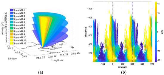
Figure 1. (a) Elevation angles of Thessaloniki radar and (b) periodic nature of radar data.

Table 1. Elevation angles of Thessaloniki radar.

Elevation Number	1	2	3	4	5	6	7	8	9	10	11	12
Angle (°)	1.2	2.0	3.0	4.1	5.3	6.6	8.2	10.1	13.1	17.1	21.1	26.1

The proposed methodology for each one of the four algorithms optionally begins by shifting data in the velocity 2D matrix, aiming to reduce the presence of large gaps that might trigger misclassifications in later steps. Due to the periodic nature of radar data, one could expand to the left and to the right the same data, but circular shifting is an approach for efficient computation and cost efficiency, as shown in Figure 1b. After realignment, the data are separated into upper and lower sections for targeted amplitude corrections. Each column is assessed for transition density, number of valid data points, and the length of uninterrupted segments. Columns with fewer abrupt jumps and extensive valid data serve as more reliable baselines.

2.1. Sine-Based Algorithms

These algorithms assume underlying sinusoidal signatures in the original data before aliasing occurs (Figure 2a), reflecting the azimuthal symmetry or periodicity of certain radar sampling geometries. The initial approach of the algorithm is to first read each radial in the velocity matrix (each row), ignoring zeros or missing values, often referenced as Not a Number (NaN) values. The procedure incrementally tests candidate sine waves over a range of amplitudes and phases (Figure 2b,c). Each gate with data at a fixed distance, which denotes a full azimuth scan, is analyzed separately and models each radial as a sinusoid that has been folded into the Nyquist velocity limit range. A generic parametric sine wave can be written as

$$S\left(\theta \right)=\alpha \sin \left(\theta +\phi \right)+b,$$

(1)

where a is the amplitude, $\phi$ the phase, $b$ a vertical offset, and $\theta$ spans the radial’s azimuthal angle or gate indices. A coarse search over ($\alpha$, $\phi$, $b$) identifies candidate solutions, each time folding out-of-range values by $\pm 2 \ast v_{Nyquist}$. After a coarse search, sampling the phase in 20° increments and the amplitude in steps of $0.2 \ast v_{Nyquist}$, a finer search re-evaluates both $\alpha$ and $\phi$ in a smaller neighborhood, around the coarse optimum, using 1° phase increments and amplitude steps of $0.1 \ast v_{Nyquist}$. To determine the best-fitting parameters, a mismatch function

$$E\left(\alpha ,\phi ,b\right)={\sum }_{\theta \in D}\left|\left(\alpha \sin \left(\theta +\phi \right)+b\right)-V_{obs}\left(\theta \right)\right|,$$

(2)

is minimized, where $D$ denotes valid non-NaN azimuth gates. The wave with the smallest mismatch metric is selected. A 180° phase shift is also checked, since $sin(\theta +\phi +180)=-sin(\theta +\phi )$. By retaining the configuration with the lowest residual error, the algorithm systematically aligns folded velocities back into the principal range.

Figure 2. (a) Aliased Doppler velocity data after aliasing, (b) test Doppler velocity data without aliasing, and (c) aliased test Doppler velocity.

Subsequently, an FFT analysis characterizes dominant frequency components across radials, providing amplitude and phase insights for refining a more global sinusoidal model. Missing values remain NaN to avoid artificially filling irretrievable data. This approach systematically addresses folding on a row-by-row basis; it can be somewhat more computationally demanding due to numerous sine-fitting steps, but it may capture azimuthal periodicities.

However, the above work acted as a start for recognizing limitations and constraints regarding the above approach. As a result, a variant algorithm is generated by squeezing data in 2D; likewise, it models each radial as a refined sine wave. After an initial coarse search for phase and amplitude (Figure 3a), folded values are corrected in a stepwise manner by bracketed sine curves.

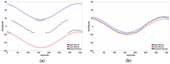
Figure 3. (a) Original and (b) dealiased Doppler velocities. Upper (blue color) and lower (red color) bracketed sine curves are in initial state in (a). By squeezing iterations and data replacements, the correct and dealiased Doppler velocity data is derived (b).

By iterating over each radial independently, the squeeze algorithm reconstructs a velocity field in which aliased samples are realigned (Figure 3b). This preserves major gradients and local patterns suggested by the sinusoidal approximation, while also minimizing abrupt discontinuities. Similarly to the sine-based approach, the squeeze algorithm first identifies a best-fit sine wave of amplitude $\alpha$ and phase $\phi$. It then creates two bounding curves:

$$U\left(\theta \right)=b+\alpha sin(\theta +\phi )+\delta \left(\theta \right),$$

(3)

$$L\left(\theta \right)=b+\alpha sin(\theta +\phi )-\delta \left(\theta \right),$$

(4)

where $\delta \left(\theta \right)$ is incrementally adjusted until it “just encloses” the observed data in each radial. The bounding curves are initialized with fixed vertical offsets of ±50 units relative to the fitted sinusoid, and $\delta \left(\theta \right)$ is then increased from this baseline in constant steps (1.0 and later 0.1) until all observed samples lie within [$L\left(\theta \right)$, $U\left(\theta \right)$]. Thus, the effective range of $\delta \left(\theta \right)$ is data-dependent, but it is important to start from a big offset. Any sample $V_{obs}\left(\theta \right)$ that crosses above $U\left(\theta \right)$ or below $L\left(\theta \right)$ is considered aliased and is brought back into range via

$$V_{corr}\left(\theta \right)=V_{obs}\left(\theta \right) \pm 2 \ast v_{Nyquist},$$

(5)

Additionally, the algorithm tries alternative phase values (e.g., $\phi$ + 180°) and picks whichever yields the fewest outliers in the final result. Iterating this procedure across all radials produces a field where velocity folds are squeezed by these bounding sine waves, preserving significant gradients and overall meteorological structure. Though more sophisticated in its multi-stage fitting, this algorithm can be beneficial when the radar data exhibit partial sinusoidal signatures across azimuth, or when large folds manifest in localized parts of the scan.

2.2. Amplitude Correction Algorithms

In contrast to the previous two strategies, this class of algorithms combines multiple quantitative checks—such as amplitude corrections, interpolation, and reference field comparisons—to identify and remove folding, similar to “DEALIASING ALONG A RADIAL” in UNRAVEL [22]. The underlying principle is to detect unrealistic velocity jumps in specific azimuth across distance (within each column of the 2D matrix), then shift out-of-range values by one or more Nyquist cycle.

An iterative amplitude correction routine compares each velocity value to a local smoothed reference. Any value deviating by more than half the Nyquist limit is shifted by a full Nyquist cycle up or down (Figure 4), effectively removing the fold.

Figure 4. (a) Original and (b) dealiased Doppler velocities of a single ray.

This algorithm segments the radar data based on distinct azimuth values in column-based data, to systematically remove velocity folds. Each column is assigned a smoothed reference ${\overline{V}}_{sm}\left(z\right)$ at range $z$. A simple approximation for ${\overline{V}}_{sm}\left(z\right)$ is a centered moving average:

$${\overline{V}}_{sm}\left(z\right) ={\displaystyle \frac{1}{2N+1}}{\sum }_{r=z-N}^{z+N}{V}_{obs}\left(r\right),$$

(6)

where $N$ is the half-width of the smoothing window, and the summation is confined to valid points. The value of the half-window $N$ is set to the rounded number of 1% of the points that exist along a gate, which depends on the number of points along a scan, regardless of the radar. Usually, the number of points along the range is larger than the points in the azimuth, enabling the moving window element to be used more efficiently in this setting. Columns with excessive discontinuities relative to their neighbors are sometimes masked or flagged to maintain spatial coherence. For each distance $z$, if the difference

$$\Delta \mathrm{V}(\mathrm{z})=\left|V_{obs}\left(z\right)-{\overline{V}}_{sm}\left(z\right)\right|,$$

(7)

exceeds a fraction of the Nyquist limit (for instance, $0.5 \ast v_{Nyquist}$), the observed value is shifted by $\pm 2 \ast v_{Nyquist}$. After this adjustment, a final pass compares each distance point to three reference fields ($V_{orig}-2 \ast v_{Nyquist}$, $V_{orig}$, $V_{orig}+2 \ast v_{Nyquist}$) to select the velocity closest to the newly corrected estimate. This multi-stage workflow ensures that folded velocities are systematically identified, corrected, and then cross-checked against the original data structure.

After iterating with all the azimuth angles (columns), discontinuous ones are flagged and masked to avoid introducing unrealistically large gradients. A two-dimensional interpolation fills remaining gaps, maintaining as much spatial continuity as possible while keeping strictly invalid data excluded. Finally, after interpolating, each velocity estimate is checked against three reference fields derived from the original velocities: one unaltered field and two fields shifted by plus or minus one Nyquist cycle. Each point in the corrected matrix is replaced with whichever reference value is closest, refining residual ambiguities. The difference between the measured and smoothed velocities is used because this algorithm can function as an intermediate step of a set of algorithms. It also operates iteratively, and as the correction proceeds, a convergence criterion monitors the number of points modified at each pass; if this number ceases to change meaningfully, the routine terminates automatically, preventing cyclic behavior and ensuring that the algorithm converges as much as possible towards a stable and physically consistent velocity solution.

By combining amplitude corrections, interpolation, and final reference comparisons, the algorithm converges on a dealiased velocity field that, although more computationally intensive, preserves essential weather features.

2.3. Expansion Algorithm

The expansion approach focuses on systematically enlarging valid velocity regions into areas affected by aliasing or missing data (Figure 5). This strategy is helpful if continuous fields of folded areas are present. Each PPI scan is processed by a procedure that detects the largest valid region. The algorithm relies on labeling connected non-NaN regions and isolating the largest such region as the core reference, using an 8-connected neighborhood that shares the same velocity sign (positive or negative), identified through a 3 × 3 convolution mask. Isolated or sign-inconsistent samples are discarded, and the largest remaining connected region is selected as the initial valid region for subsequent expansion, through an iterative process. At each iteration, it identifies the outer perimeter of the core region of valid (non-NaN) velocities and then calculates the local mean around these perimeter points. Within each iteration, the outer perimeter of this valid region is located using a neighborhood-based convolution mask. For a perimeter point $(\mathrm{i},\mathrm{j})$, a typical 3 × 3 neighborhood mean ${\overline{V}}_{3\times 3}\left(i,j\right)$ is

$${\overline{V}}_{3\times 3}\left(i,j\right)={\displaystyle \frac{1}{\left|{\Omega }_{3\times 3}\right|}}{\sum }_{\left(p,q\right)\in {\Omega }_{3\times 3}(i,j)}{V}_{obs}(p,q),$$

(8)

where ${\Omega }_{3\times 3}(i,j)$ is the set of valid neighbors in the immediate 3 × 3 block centered at $(\mathrm{i},\mathrm{j})$, and $\left|{\Omega }_{3\times 3}\right|$ is the number of valid points in that block. Any perimeter points whose velocity differs substantially from their local mean are considered aliased. Specifically, if

$$\left|V_{obs}\left(i,j\right)-{\overline{V}}_{3\times 3}\left(i,j\right)\right|>\Delta u_{threshold},$$

(9)

the observed velocity $V_{obs}\left(i,j\right)$ is shifted by $\pm 2 \ast v_{Nyquist}$. Once these perimeter velocities are corrected, they become part of the valid region, and the perimeter is recalculated. This iterative expansion continues until no further NaN areas remain or no additional points can be corrected, thereby filling in large data gaps with newly dealiased velocities. To ensure full coverage, the expansion algorithm can iterate multiple times if unfilled areas remain. It can produce a more complete and coherent velocity field in highly aliased or data-sparse scans. The replacement of one Nyquist interval ($\pm 2 \ast v_{Nyquist}$) may not be adequate enough in highly aliased datasets, highlighting the need to repeat the process in an iterative mode.

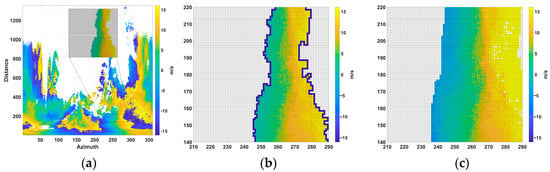
Figure 5. (a) Initial state Doppler velocity data. (b) Initial state Doppler velocity data with step of expansion with blue color. (c) Expanded state of Doppler velocities.

2.4. Convolution Algorithm

A local neighborhood averaging process is performed using a geometric shape (tunable size, box, or circular kernel), which is convolved with the velocity field to compute local mean values. A user-defined kernel size (either an $n \times n$ box or a circular mask of radius $r$) is used, and the mean value is computed only over non-NaN neighbors, making it a NaN-aware local averaging operator rather than a fixed traditional mean filter. The algorithm compares each velocity measurement against its corresponding local mean and identifies any values exceeding the Nyquist velocity by flagging them as aliased. Let $V_{obs}\left(i,j\right)$ be the observed velocity at grid point $\left(i,j\right)$, and let $\overline{V}\left(i,j\right)$ represent the local mean derived by convolving the velocity field with a kernel K. The local mean is computed by summing valid (non-NaN) neighboring values and dividing them by the number of valid neighbors. One straightforward representation is:

$$\overline{V}\left(i,j\right)= {\displaystyle \frac{{\sum }_{\left(m,n\right)\in \Omega }K\left(m,n\right) ·V_{obs}(i+m,j+n)}{{\sum }_{\left(m,n\right)\in \Omega }K\left(m,n\right) }},$$

(10)

where Ω denotes the set of indices in the kernel neighborhood around $\left(i,j\right)$. These flagged velocities are shifted by adding or subtracting one Nyquist interval ($\pm 2 \ast v_{Nyquist}$). In each iteration, a mask tracks valid (non-missing) data, ensuring that pixels identified as missing do not skew the local mean calculations (Figure 6). Convolution with the chosen kernel yields both the local sums of valid velocity data and the local counts of non-missing pixels.

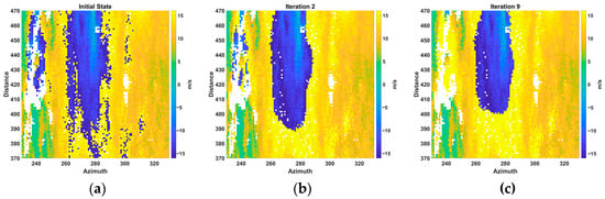
Figure 6. (a) Initial aliased state, (b) state after 2 iterations, and (c) state after 9 iterations of Doppler velocity data.

After computing the local mean, the algorithm compares $V_{obs}\left(i,j\right)$ against $\overline{V}\left(i,j\right)$. If the deviation $\left|V_{obs}(i,j)-\overline{V}\left(i,j\right)\right|$ exceeds a specified threshold (set equal to the Nyquist velocity), the value is deemed aliased. The corrected velocity $V_{corr}\left(i,j\right)$ is then updated by adding or subtracting 2 times the Nyquist value, to bring it closer to the local mean:

$$V_{corr}\left(i,j\right)= V_{obs\left(i,j\right)} \pm 2 \ast v_{Nyquist},$$

(11)

where the sign is chosen to minimize $\left|V_{corr}(i,j)-\overline{V}\left(i,j\right)\right|$. This process continues until the algorithm converges and no additional points are flagged as aliased. As an example, in Figure 6, the results after 2 and 9 iterations are shown as part of a convergence process out of 190 iterations.

3. Performance Evaluation of Individual Algorithms

By evaluating the performance of the four multiple-Doppler-velocity dealiasing techniques described, their advantages and limitations are described by applying them in real radar data, with the aim of generating a Combined Algorithm Approach. The test case of 10 July 2019 was selected for this experiment because it is characterized by significant velocity aliasing due to (a) extreme wind velocities, (b) suboptimal Pulse Repetition Frequency (PRF) settings, and (c) frontal activity followed by a non-sinusoidal uniform pattern (Figure 7 and Figure 8b). The frontal activity is shown in Figure 7, as well as the Chalkidiki area near Thessaloniki’s radar Doppler velocities (Figure 8). A Nyquist value of 16.05 m/s, as calculated from the data, is evidence of a low-PRF setting. The data presented in this Section were derived from only one elevation angle of approximately 2.87 degrees, which is the third elevation angle for the specific radar. The Software used for development and implementation is MATLAB version 2017a.

Figure 7. Surface pressure chart analysis of Europe combined with EUMETSAT MSG SEVIRI IR 10.8 μm brightness temperatures for 9 July 2019, 12:00 UTC.

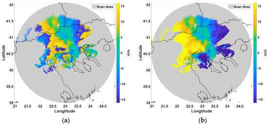
Figure 8. (a) Original aliased and (b) fully dealiased Doppler velocities over Chalkidiki area from the Thessaloniki radar in m/s.

The initial aliased dataset, shown in Figure 8a, presents the Doppler velocity field before any corrections were applied. The fully dealiased dataset is also shown in Figure 8b, retrieved by manually correcting each row and column of the original 2D matrix, as a best effort for reference and validation. This manual correction refers to applying the above algorithms sequentially while visually identifying the least aliased regions. Although this approach does not reconstruct the true unambiguous dataset—multiple possible datasets may map to the originally aliased velocities [19]—it represents the best estimate of a dealiased dataset. The manual correction took into consideration the visual continuity of data as well as the sinusoidal patterns that occur, along with the frontal activity. The aliasing is evident, with multiple regions displaying velocity discontinuities where velocity folding has occurred. This highlights the necessity of post-processing techniques to ensure accurate wind field retrievals. The data were derived from a low-PRF radar, where aliasing was prominent (Figure 8a), while high-PRF radars exhibit minimal aliasing, reducing the need for dealiasing algorithms altogether. This reinforces the idea that optimizing PRF should be the first step before relying on post-processing techniques.

For each individual algorithm, the output datasets were compared against the manually dealiased dataset qualitatively and quantitatively by comparing them visually and mathematically, respectively. The mathematical approach demonstrates the percentage of match between the manually dealiased dataset and the output of each algorithm, shown in Table 2.

Table 2. Individual algorithm comparison.

Algorithm	Sine Approach	Amplitude Correction	Expansion	Convolution
Effectiveness in Aliased Regions	Low	Moderate	Moderate–High	High
Computational Cost	Low	Moderate	Moderate	High
Artifact Introduction	Moderate (Radial Artifacts)	Low	Low	Minimal
Performance in Sparse Data Areas	Poor	Moderate	Moderate	Good
Continuity Preservation	Moderate	Good	Very Good	Excellent
Best Use Case	Limited applications	Basic dealiasing	Better for structured systems	Best single-algorithm choice
Physics	Physics based	Independent	Independent	Independent
Disadvantages	Not efficient with non-uniform wind fields	Does not work well in areas with big gaps	When expanding to larger area, it might falsely jump to $\pm 2 \ast v_{Nyquist}$	Enhances limited areas and smooths
Geometry	Distance scan-based	Ray based	Independent	Independent
Iterations	Fixed steps	Fixed steps	Iterative	Iterative
Score (%)	72.8393	96.2532	87.0248	63.1977

The performance evaluation was conducted on a system equipped with an Intel Core i5-6300U processor (2 physical cores, 4 logical threads, 2.40 GHz base frequency), 8 GB of RAM, and running 64-bit Microsoft Windows 11 Pro. Across all methods, computational demand varies according to the underlying algorithmic structure (Table 3). The expansion method exhibits $O\left(n^3\right)$ complexity because each growth step scans the entire matrix $O\left(n^2\right)$ and this process may repeat up to n times. The amplitude correction method is scaled as $O\left(n^2\right)$, since both amplitude correction and interpolation involve full-matrix operations. The sine approach method also follows $O\left(n^2\right)$ behavior, as the work required for each radial gate grows quadratically with the number of points. Finally, the convolution-based approach remains $O\left(n^2\right)$, because each iteration applies a fixed-size kernel across the entire matrix, and the kernel size does not scale with the domain.

Table 3. Individual algorithm complexity and runtime comparison.

Algorithm	Complexity	Runtime (s)
Expansion	O(n3)	23.4
Amplitude Correction	O(n2)	16.3
Sine Approach	O(n2)	17.3
Convolution	O(n2)	43.1

The first approach tested was the sine-based algorithm (Figure 9a). The algorithm does not completely removes aliasing, particularly in regions where data are sparse—areas that do not have a full set of data and have many discontinuities, in such a way that it cannot be clear if the data are aliased or not. A radial banding effect is observed, indicating that this approach struggles in areas where velocity gradients are steep regarding the azimuth.

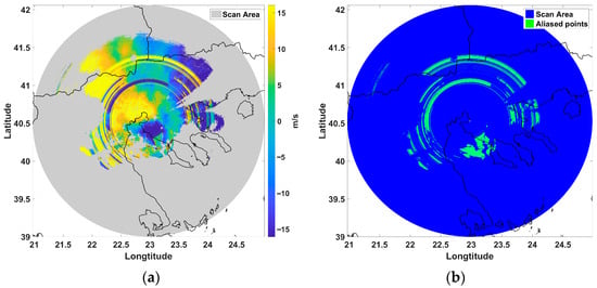
Figure 9. (a) Sine-based algorithm results (m/s) and (b) residuals from comparison with fully dealiased dataset (scan area blue, residuals green).

The sine-based algorithm is effective in data that follow a smooth wind flow, like the upper-level winds, rather than surface wind fields, where fronts might occur. This is because the frontal activity is followed by a non-sinusoidal uniform pattern, as in higher altitudes, where the wind flow has large area characteristics.

The amplitude correction algorithm (Figure 10a) provided a notable improvement from the previous two approaches. In this case, the correction was more structured and consistent, with fewer artificial distortions introduced (Figure 10b). While aliasing was reduced in several key areas, some folded velocities remained, in regions where frontal activity is present, according to Figure 7.

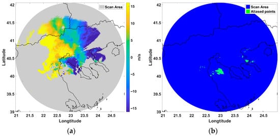
Figure 10. (a) Amplitude correction algorithm results (m/s) and (b) residuals from comparison with fully dealiased dataset (scan area blue, residuals green).

The expansion algorithm (Figure 11a) further improved upon the results of the physics-based approaches in several regions. This algorithm preserved velocity continuity effectively, particularly in regions where wind structures were well-defined, such as in areas where the wind does not change direction, as opposed to areas that have frontal activity and where the wind current changes its direction. However, aliasing persisted in areas where data coverage was limited, highlighting a common challenge faced by dealiasing algorithms. The improvement over previous algorithms suggests that expansion-based dealiasing can be an effective approach when data availability is high. The main challenge for this algorithm is when the expansion is performed from inner to outer data, and the inner data are less than the outer in summary. This demand may introduce artifacts in the expansion logic.

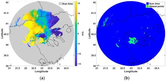
Figure 11. (a) Expansion algorithm results (m/s) and (b) residuals from comparison with fully dealiased dataset (scan area blue, residuals green).

Finally, the convolution algorithm (Figure 12a) demonstrated satisfactory results. Aliasing was significantly reduced, and the velocity field appeared smoother and more continuous compared to previous approaches in specific regions. However, in regions with limited azimuthal and radial data, aliasing effects were still present (Figure 12b). These findings indicate that convolution-based dealiasing is a strong candidate for operational applications but still requires complementary techniques in challenging scenarios, such as frontal activity and in instances of local cyclonic phenomena, where winds cannot be described adequately due to the distance of measurements relative to the radar site and radar beam expansion.

Figure 12. (a) Convolution algorithm results (m/s) and (b) residuals from comparison with fully dealiased dataset (scan area blue, residuals green).

4. Combined Algorithm Approach—Discussion

The Combined Algorithm Approach is the result of reviewing the sequential algorithms described above, recognizing the limitations of individual algorithms, and leveraging the strengths of multiple algorithms to generate an optimized velocity field. The sequence of the algorithms followed in this study—squeeze, convolution, and, finally, amplitude correction—to create a combined approach was selected based on the residual aliasing of each algorithm discussed above. The expansion algorithm, although it yields promising results, relies solely on connected areas and thus has been omitted from the combined approach. As an example, using data derived from only one elevation angle of approximately 2.87 degrees, which is the third elevation angle for the specific radar, the final result demonstrates a fully dealiased dataset, where all significant aliasing artifacts have been removed while maintaining spatial continuity. The final output, shown in Figure 13a, achieved a score of 96.356%, surpassing the performance of any individual algorithm (Table 2).

Figure 13. (a) Dealiased Doppler velocities by combined approach (m/s), (b) fully dealiased dataset (m/s), and (c) residuals from comparison with fully dealiased dataset (scan area blue, residuals green).

The residuals from comparing the velocity fields in Figure 13c demonstrate a significant reduction in both the magnitude and spatial extent of remaining aliasing artifacts, marking a substantial improvement over any individual algorithm approach. The continuity of the velocity structures is preserved, making the dataset suitable for assimilation into numerical weather prediction models.

Single-algorithm dealiasing approaches exhibit significant limitations. The sine approach algorithms introduced artificial distortions, making them unsuitable for high-accuracy dealiasing. The amplitude correction, expansion, and convolution algorithms performed better but still struggled in regions with limited data. The amplitude correction algorithm provided the best single-algorithm performance. This approach was the most effective in reducing aliasing while maintaining velocity continuity. However, some aliasing persisted in regions where frontal activity was present, indicating that no single algorithm is universally optimal. A detailed evaluation of individual algorithms revealed key strengths and limitations.

A multi-algorithm approach is essential for optimal dealiasing. By combining multiple algorithms, aliasing was fully corrected across the entire radar scan. The final dataset demonstrated superior accuracy, continuity, and robustness, making it the most suitable for operational use.

Several challenges emerged during the application of the individual dealiasing algorithms. Iterative algorithms provided more accurate dealiasing but required higher computational time, making them potentially impractical for real-time applications. In contrast, sine-based algorithms produced faster results but were visually inferior, often introducing unrealistic velocity structures. The algorithms generally performed well in data-rich regions, but their effectiveness decreased in areas with limited azimuthal and range coverage, as well as where wind velocities do not follow a smooth flow pattern. This suggests that dealiasing success is highly dependent on data availability, scan completeness, and weather conditions.

Computational cost is a major issue for iterative approaches, which require multiple-step passes to converge on a solution. This poses a challenge for operational meteorology, where real-time processing is crucial. Regions with sparse data, particularly at greater distances from the radar or in low-reflectivity areas, also negatively impact dealiasing performance. When azimuthal or radial gaps are present, algorithms struggle to infer the correct velocities, leading to increased uncertainty. No single algorithm failed outright, but each exhibited reduced performance in data-sparse environments. Moreover, the results from the UNRAVEL methodology are compared to the applied combined approach of the algorithms. As stated in the previous sections, manually corrected data are referenced as ground truth as an attempt to perform a comparison of the Combined Approach Algorithms, UNRAVEL, and the original aliased data, since there are no valid true dealiased data. The Combined Approach Algorithms surpassed UNRAVEL, as shown in Figure 14 (Table 4). The original data, the results from UNRAVEL, the results from the Combined Approach Algorithms, and the results from the manual correction are shown in Figure 15.

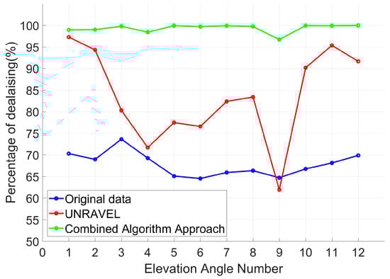
Figure 14. Comparison results between fully dealiased data versus (a) original aliased data (blue line), (b) UNRAVEL results (red line), and (c) Combined Algorithm Approach results (green line).

Table 4. Results comparison.

Elevation Angle Number	1	2	3	4	5	6	7	8	9	10	11	12
Original Data	70.29	68.96	73.64	69.26	65.08	64.53	65.92	66.35	64.71	66.76	68.13	69.88
UNRAVEL	97.29	94.32	80.32	71.70	77.48	76.59	82.38	83.41	61.93	90.19	95.38	91.67
Combined Algorithm Approach	98.97	99.02	99.79	98.44	99.93	99.71	99.91	99.75	96.73	99.95	99.91	100.00

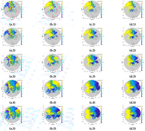
Figure 15. Data from (a) original aliased data, (b) UNRAVEL algorithm, (c) sequential new algorithm, and (d) fully dealiased data. Each row represents the elevation angle number, based on Table 1.

Finally, while dealiasing algorithms are essential, they are not a substitute for proper radar configuration. While they remain necessary in many operational settings, optimizing PRF settings should be the initial action for improving Doppler velocity retrievals. In cases where aliasing is unavoidable, the choice of algorithm should balance computational efficiency and accuracy, depending on the specific use case.

5. Concluding Remarks

This study applied a set of distinct dealiasing algorithms to a real radar case from Thessaloniki radar, Greece (10 July 2019), to evaluate their performance in the presence of varying meteorological and radar configuration conditions. The results show that all four algorithms improved data quality, but their effectiveness varied based on the geometry of the weather systems, elevation angles, and data availability in certain regions.

Individual testing of the four algorithms demonstrated varying levels of effectiveness, with iterative approaches yielding better results at the cost of computational time, and sine-based algorithms being less effective despite faster processing.

The integration of a combined approach of multiple dealiasing algorithms yields a significantly improved dealiased dataset, surpassing the performance of any single algorithm approach discussed across multiple PPI scans. The limitations of individual algorithm approaches underscore the necessity of a combined approach, especially for data-sparse or complex regions. Operational velocity dealiasing requires a multi-algorithm approach and optimized radar configuration, taking into account computational demands.

Future research should explore the integration of machine learning-based dealiasing techniques, leveraging large datasets to improve performance in regions with sparse data. Additionally, adaptive PRF strategies, where PRF is dynamically adjusted based on elevation angle and wind conditions, could also minimize aliasing and improve radar-based wind retrievals. Incorporating a quality control (QC) framework—assigning confidence levels to dealiased pixels—could enhance data reliability for radar data assimilation.

References

- Maiello, I.; Ferretti, R.; Gentile, S.; Montopoli, M.; Picciotti, E.; Marzano, F.S.; Faccani, C. Impact of radar data assimilation for the simulation of a heavy rainfall case in central Italy using WRF–3DVAR. Atmos. Meas. Tech. 2014, 7, 2919–2935. [Google Scholar] [CrossRef]
- Mazzarella, V.; Maiello, I.; Ferretti, R.; Capozzi, V.; Picciotti, E.; Alberoni, P.P.; Marzano, F.S.; Budillon, G. Reflectivity and velocity radar data assimilation for two flash flood events in central Italy: A comparison between 3D and 4D variational methods. Q. J. R. Meteorol. Soc. 2020, 146, 348–366. [Google Scholar] [CrossRef]
- Spyrou, C.; Varlas, G.; Pappa, A.; Mentzafou, A.; Katsafados, P.; Papadopoulos, A.; Anagnostou, M.N.; Kalogiros, J. Implementation of a Nowcasting Hydrometeorological System for Studying Flash Flood Events: The Case of Mandra, Greece. Remote Sens. 2020, 12, 2784. [Google Scholar] [CrossRef]
- Honda, T.; Amemiya, A.; Otsuka, S.; Lien, G.-Y.; Taylor, J.; Maejima, Y.; Nishizawa, S.; Yamaura, T.; Sueki, K.; Tomita, H.; et al. Development of the real-time 30-s-update big data assimilation system for convective rainfall prediction with a phased array weather radar: Description and preliminary evaluation. J. Adv. Model. Earth Syst. 2022, 14, e2021MS002823. [Google Scholar] [CrossRef]
- Wang, H.; Sun, J.; Fan, S.; Huang, X. Indirect Assimilation of Radar Reflectivity with WRF 3D-Var and Its Impact on Prediction of Four Summertime Convective Events. J. Appl. Meteor. Climatol. 2013, 52, 889–902. [Google Scholar] [CrossRef]
- Samos, I.; Flocas, H.; Louka, P.; Gofa, F.; Emmanouil, A. Velocity estimation of thunderstorm movement and dealiasing of single Doppler radar during convective events. Acta Geophys. 2024, 72, 3751–3772. [Google Scholar] [CrossRef]
- Mazzarella, V.; Ferretti, R.; Picciotti, E.; Marzano, F.S. Investigating 3D and 4D variational rapid-update-cycling assimilation of weather radar reflectivity for a heavy rain event in central Italy. Nat. Hazards Earth Syst. Sci. 2021, 21, 2849–2865. [Google Scholar] [CrossRef]
- Sun, J. Convective-scale assimilation of radar data: Progress and challenges. Q. J. R. Meteorol. Soc. 2005, 131, 3439–3463. [Google Scholar] [CrossRef]
- Ivanov, S.; Michaelides, S.; Ruban, I.; Charalambous, D.; Tymvios, F. Impact of radar data assimilation on simulations of precipitable water with the Harmonie model: A case study over Cyprus. Atmos. Res. 2021, 253, 105473. [Google Scholar] [CrossRef]
- Radi, A.; Al-Katheri, A.A.; Dhanhani, A. Tuning of WRF 3D-VAR Data Assimilation System over Middle-East and Arabian Peninsula. Available online: https://citeseerx.ist.psu.edu/document?repid=rep1&type=pdf&doi=996008b61f91b45da8cf53b30ab8c38aa24b682e (accessed on 19 January 2025).
- Sugimoto, S.; Crook, N.A.; Sun, J.; Xiao, Q.; Barker, D.M. An Examination of WRF 3DVAR Radar Data Assimilation on Its Capability in Retrieving Unobserved Variables and Forecasting Precipitation through Observing System Simulation Experiments. Mon. Wea. Rev. 2009, 137, 4011–4029. [Google Scholar] [CrossRef]
- Liang, X. An Integrating Velocity–Azimuth Process Single-Doppler Radar Wind Retrieval Method. J. Atmos. Ocean. Technol. 2007, 24, 658–665. [Google Scholar] [CrossRef]
- Wang, H.; Sun, J.; Zhang, X.; Huang, X.; Auligné, T. Radar Data Assimilation with WRF 4D-Var. Part I: System Development and Preliminary Testing. Mon. Wea. Rev. 2013, 141, 2224–2244. [Google Scholar] [CrossRef]
- Giannaros, T.M.; Kotroni, V.; Lagouvardos, K. WRF-LTNGDA: A lightning data assimilation technique implemented in the WRF model for improving precipitation forecasts. Environ. Model. Softw. 2016, 76, 54–68. [Google Scholar] [CrossRef]
- Barker, D.M.; Huang, W.; Guo, Y.; Bourgeois, A.J.; Xiao, Q.N. A Three-Dimensional Variational Data Assimilation System for MM5: Implementation and Initial Results. Mon. Wea. Rev. 2004, 132, 897–914. [Google Scholar] [CrossRef]
- Earth System Modeling, Data Assimilation and Predictability Atmosphere, Oceans, Land and Human System. ISBN 9781107009004. Available online: http://www.cambridge.org/9780521791793 (accessed on 1 February 2025).
- Samos, I.; Flocas, H.; Louka, P. A Background Error Statistics Analysis over the Mediterranean: The Impact on 3DVAR Data Assimilation. Environ. Sci. Proc. 2023, 26, 158. [Google Scholar] [CrossRef]
- Sun, J.; Wang, H. Radar Data Assimilation with WRF 4D-Var. Part II: Comparison with 3D-Var for a Squall Line over the U.S. Great Plains. Mon. Wea. Rev. 2013, 141, 2245–2264. [Google Scholar] [CrossRef]
- He, G.; Sun, J.; Ying, Z.; Zhang, L. A Radar Radial Velocity Dealiasing Algorithm for Radar Data Assimilation and its Evaluation with Observations from Multiple Radar Networks. Remote Sens. 2019, 11, 2457. [Google Scholar] [CrossRef]
- Xu, Q.; Nai, K.; Liu, S.; Karstens, C.; Smith, T.; Zhao, Q. Improved Doppler Velocity Dealiasing for Radar Data Assimilation and Storm-Scale Vortex Detection. Adv. Meteorol. 2013, 10, 562386. [Google Scholar] [CrossRef]
- Dong, X.; Zhao, X.; Chen, Z.; Li, Y.; Wang, S. Doppler Velocity De-Aliasing Based on Lag-1 Cross-Correlation for Dual-Polarization Weather Radar. IEEE Geosci. Remote Sens. Lett. 2024, 21, 1–5. Available online: https://ieeexplore.ieee.org/document/10400523 (accessed on 2 February 2025). [CrossRef]
- Louf, V.; Protat, A.; Jackson, R.C.; Collis, S.M.; Helmus, J. UNRAVEL: A Robust Modular Velocity Dealiasing Technique for Doppler Radar. J. Atmos. Ocean. Technol. 2020, 37, 741–758. [Google Scholar] [CrossRef]
- Feldmann, M.; James, C.N.; Boscacci, M.; Leuenberger, D.; Gabella, M.; Germann, U.; Wolfensberger, D.; Berne, A. R2D2: A Region-Based Recursive Doppler Dealiasing Algorithm for Operational Weather Radar. J. Atmos. Ocean. Technol. 2020, 37, 2167–2183. Available online: https://infoscience.epfl.ch/entities/publication/cb1ad4ca-7b55-479e-b75e-beb890820324 (accessed on 3 March 2025). [CrossRef]
- Zou, H.; Liang, X.; Wu, S.; Yin, J. A Dealiasing Scheme of Doppler Radar Velocity Based on Polynomial Fitting. IEEE Trans. Geosci. Remote Sens. 2024, 62, 1–10. Available online: https://scispace.com/papers/a-dealiasing-scheme-of-doppler-radar-velocity-based-on-46r2dp5pld (accessed on 3 March 2025). [CrossRef]
- Kim, H.; Cheong, B. Robust Velocity Dealiasing for Weather Radar Based on CNN. Remote Sens. 2023, 15, 802. [Google Scholar] [CrossRef]
- Veillette, M.S.; Kurdzo, J.M.; Stepanian, P.M.; McDonald, J.; Samsi, S.; Cho, J.Y.N. A Deep Learning–Based Velocity Dealiasing Algorithm Derived from the WSR-88D Open Radar Product Generator. Artif. Intell. Earth Syst. 2023, 2, e220084. [Google Scholar] [CrossRef]
Disclaimer/Publisher’s Note: The statements, opinions and data contained in all publications are solely those of the individual author(s) and contributor(s) and not of MDPI and/or the editor(s). MDPI and/or the editor(s) disclaim responsibility for any injury to people or property resulting from any ideas, methods, instructions or products referred to in the content. |
© 2025 by the authors. Licensee MDPI, Basel, Switzerland. This article is an open access article distributed under the terms and conditions of the Creative Commons Attribution (CC BY) license (https://creativecommons.org/licenses/by/4.0/).