Highlights
What are the main findings?
- Remote SST has a strong relationship with the in situ SST but consistently showed a cold bias.
- Remote SST aligned better with the near-surface layer than the skin layer.
What are the implications of the main findings?
- Rain-related bias reversals indicate environmental dependencies worth exploring.
- The bulk-like behaviour of satellite SST strengthens its operational value.
Abstract
Validating satellite-derived sea surface temperature (SST) requires resolving spatial and vertical mismatches between remotely sensed measurements and traditional in situ observations. This study evaluates the bias between infrared-based satellite SST and high-resolution in situ measurements collected in the North Sea using the autonomous surface vehicle (ASV) HALOBATES. The ASV enables the direct sampling of the ocean skin layer via a rotating glass disc system, alongside near-surface layer (NSL, 1 m depth) measurements using a flow-through system. Across 37 missions conducted between 2022 and 2023, we quantified biases in our approach and performed match-ups with a level-4 SST product for the North and Baltic Seas. Satellite SST showed strong correlations with in situ observations (r > 0.98), with Deming regression slopes approaching unity for all platforms. Despite this agreement, satellite SST exhibited a consistent cold bias. The mean differences were −0.44 ± 0.60 °C for the skin layer and −0.40 ± 0.52 °C for the NSL. The RMSE values were 0.75 °C for the skin layer and 0.66 °C for the NSL, indicating that satellite SST more closely reflects temperatures at 1 m than those at the skin layer. These findings highlight the importance of depth-resolved in situ measurements for improving remote SST validation.
1. Introduction
Satellite-based sea surface temperature (SST) provides a great understanding of various dynamics of the ocean. This includes ocean circulation, heat transport, and air–sea interactions [1]. These measurements are pivotal for understanding climate dynamics, as SST influences weather patterns, ocean–atmosphere coupling, and global biogeochemical cycles. SST plays a crucial role in shallow seas, such as the North Sea (95 m on average), which are highly prone to warming and sea-level rise, making them critical for regional climate assessments. Additionally, SST corrections in gas exchange models have significant implications for global air–sea CO2 and oxygen flux estimates, impacting the accuracy of climate prediction [2].
Satellite data providers validate their measurements primarily using in situ data from buoys, moorings, and Argo floats. However, these sources often collect data from depths greater than the penetration depth of satellite radiometers. Satellite SST is obtained from the first few micrometres and millimetres of the sea surface, commonly referred to as the skin temperature or, in some cases, the subskin temperature. However, the skin temperature is influenced by rapid surface processes, such as heat flux, evaporation, and wind stress, affecting only the top few millimetres of the ocean [3]. In contrast, in situ measurements from buoys and other devices, which are typically submerged at 1 m or more below the surface, capture a more stable near-surface layer (NSL) temperature that integrates and smoothens these rapid fluctuations [4]. Since the satellite products are often the result of an instantaneous capture of the skin temperature at a point in time, the radiometers may capture the SST at a point of rapid change occurrence which will not be visible in the underlying water. This highlights a mismatch between the remotely sensed skin temperatures obtained via satellite and in situ measurements.
This mismatch exists not only on the horizontal scale [5] but also on the vertical scale. The horizontal scale mismatch arises from a typical resolution of >2 km of remotely sensed data compared with local in situ measurements. The horizontal scale mismatch is due to the lack of technology for the non-local measurement and continuous measurement of the skin layer with a thickness of <1 mm [6,7], which is most similar to the penetration depth of signals from infrared and microwave radiometers on satellites [1]. The vertical mismatch arises from comparing remotely sensed data with a penetration depth of less than 1 mm to in situ measurements from a depth greater than 1 m. Infrared radiometers have a shallow penetration depth of approximately 10–20 µm, whereas microwave radiometers can penetrate up to 1 mm [8]. The Group for High-Resolution Sea Surface Temperature defines the penetration depth of infrared radiometers as the skin SST and that of microwave radiometers as the subskin SST. The subskin is the layer just beneath the skin layer, with a thickness of up to 1 mm, and is affected by molecular and viscous heat transfer processes [2].
Multiple studies have reported a root-mean-square error of 0.6 °C to 1.0 °C between satellite derived SST and in situ observations from the upper 10 m across different oceanic regions [9,10,11,12,13]. In most of these kinds of studies, in situ data are obtained from point measurements [13] or flow-through systems [14] and depths greater than a metre, which highlights the need for a comparative study with data from the skin layer. Ship intakes provide data at approximately 1–7 m in regions like the eastern Canadian shelf and around the Korean Peninsula [10,12]. Moored buoys sample depths of 1–10 m in the North Sea, Baltic Sea, and Arctic [14,15]. Benthic loggers record bottom temperatures off UK coastlines and La Parguera reefs [11,13]. These cover coastal and shelf seas, including British Columbia [16]. In most of these cases, a satellite grid of greater than 2 km is represented by a single or couple of point measurements, creating a great horizontal mismatch. The use of deeper depth measurements ranging from 1 m to 10 m also creates a vertical mismatch, as the satellite-derived SST originates from shallow depths of less than 1 mm. Similar challenges exist for land surface temperature, where satellite retrievals are validated against ground-based meteorological stations and soil temperature sensors to account for near-surface stratification and diurnal variability [17].
We present measurements from the state-of-the-art autonomous surface vehicle (ASV) HALOBATES, which can measure temperatures from the skin and near-surface layers (NSLs). This configuration allows for the simultaneous measurement of the skin and NSL, bridging the gap between satellite penetration depths and conventional in situ sensors. Data were obtained from the German Bight of the North Sea across all seasons between 2022 and 2023. We compared the in situ skin and NSL temperature data with the satellite remotely sensed data of the area. The main objective was to ascertain whether the SST from the satellite product accurately reflects the in situ temperature from its penetration depth (skin layer) or that of relatively deeper waters from the NSL. Prior to match-up analysis, we present the errors associated with our data acquisition techniques and analysis approaches.
2. Material and Methods
2.1. Study Area and Period
The in situ data were obtained from four field campaigns in the southeastern part of the North Sea (Figure 1) aboard the research vessel (RV) Heincke. The expeditions used in the study are the HE598 from 2–20 May 2022, HE609 from 5–23 October 2022, HE614 from 2–22 March 2023, and HE626 from 21 July–8 August 2023. For clarity, the data for March are referred to as winter, whereas those for May, July, and October are referred to as spring, summer, and autumn, respectively. For this study, we present the results from 37 daily missions across all seasons, with a total of approximately 227 h of observation. Each mission is referred to as a specific station. Figure 2 shows a typical track of the HALOBATES.
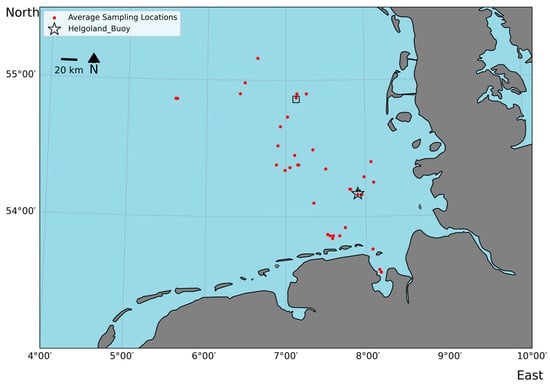
Figure 1.
Study area within the North Sea, with red dots indicating the average sampling position of HALOBATES. The black star represents the position of an oceanographic observation buoy near the island of Helgoland. The black rectangular box shows the study area, with the mission path in Figure 2.
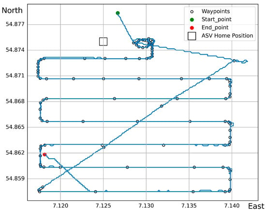
Figure 2.
A typical automated mission path of HALOBATES, following a set of waypoints during one of the deployments in the North Sea. Blue line is the track of HALOBATES as it moves from one waypoint to the next. On this day, HALOBATES did the same track twice.
At most stations, we obtained data in a defined area by setting waypoints for the HALOBATES (Figure 2). However, HALOBATES was occasionally allowed to drift with the currents. Sea state was the primary factor in determining whether to select an automated mission or a drifting approach. Wavy conditions introduce uncertainty to the data collection process when not drifting due pitching, heaving, rolling, and possible splashing.
2.2. Data
HALOBATES is equipped with multiple sensors, including seven Conductivity, Temperature, and Depth (CTD) sensors and six temperature probes. It also has a set of meteorological sensors on its bridge. The details of the design and operation of HALOBATES are highlighted in a technical paper [18]. Two approaches were used to measure water temperature. The first uses a flow-through system in which water is pumped from various depths to CTDs mounted on HALOBATES. A ladder is mounted at the bow holding tubes at different depths to pump the water from defined depths to the CTDs. HALOBATES has a state-of-the-art rotating glass disc assembly (Figure 3) to sample the skin layer. The glass discs, through the phenomena of surface tension and adhesion, skim the skin layer from the surface in a well-established technique [19,20]. A set of wipers located between the glass discs collects the water, and this is pumped by a peristaltic pump to the CTDs. The second approach is in situ measurements, with the temperature probes mounted at the various depths of interest on the same ladder. The second approach involves no sampling of the skin layer because it is technically not feasible to measure the skin layer with the probe directly.
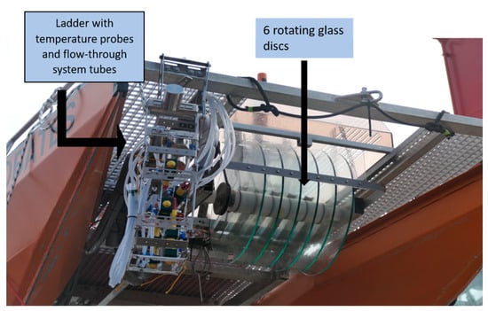
Figure 3.
Image of HALOBATES showing the six glass discs’ assembly as well as the ladder (rolled up for safe deployment) with the six temperature probes and tubes for the flow-through system installed at different heights.
Temperature probes RBRsolo3 (RBR Ltd., Ottawa, ON, Canada) and CTD OS310 (Idronaut S.r.l, Brugherio, Italy) were used for this study. The CTD’s temperature has an accuracy of ±0.0015 °C, while the temperature probe’s accuracy is ±0.002 °C. Unlike standard models, where the thermistor sits outside the cell, the CTDs were customised with the thermistor placed in the conductivity cell. We do not use an infrared camera to keep in situ data acquisition the same for all depths and for the cross-comparison for buoy measurements. Our approach is consistent with the comparisons performed by providers of remotely sensed data, that is, comparing infrared remote data with in situ measurements taken by submersible temperature probes. The measurement frequency for the temperature probes and CTDs was set to 1 Hz, but, for this study, data were averaged to daily levels for consistency with overpasses of satellites and their daily products.
Measurements were conducted at seven discrete depths from the skin to 1 m. In this study, we define the NSL to be at a depth of 1 m. Data for the skin layer and NSL were used in this study. The skin layer was chosen because its thickness is most similar to the penetration depth of infrared (~10–20 µm) and microwave radiometers (~1 mm) [8]. The 1 m depth was used because it is a well-accepted reference choice for depicting the ocean’s heat reservoir [21]. Another reason for opting for the 1 m depth and not the intermediate depth is its wide use in the correction of satellite-derived SST, as most in situ data used in the process are from similar depths. Thus, the intermediate layers served as a transition zone between the two layers. We cannot collect the subskin layer, as an increased rotational speed of the glass discs would not help, as the gravity of such a thick layer on the discs will break the adhesion forces. The complete datasets of these campaigns are available in the PANGAEA data repository [22,23,24,25].
We used data from an oceanographic observation buoy to provide an alternative comparison to our match-up analysis. The buoy is located close to the island Helgoland (54.167N, 7.9E; see Figure 1) at a depth of 1 m with an hourly temporal resolution. This buoy was in a relatively central location from all our deployment stations during the study period, making it suitable to compare with, as opposed to others in the North Sea. Buoy data were obtained from the Oceanography Department of the German Federal Maritime and Hydrographic Agency (BSH). The buoy data was collated within the Copernicus Marine Service (In Situ) and EMODnet collaboration framework. Data is made freely available by the Copernicus Marine Service and the programs that contribute to it..
The remotely sensed data used in this study are derived from various infrared radiometers. The level-4 satellite data (Baltic Sea—Diurnal Subskin Sea Surface Temperature Analysis) version 2 were developed by the Danish Meteorological Institute, Copenhagen, Denmark [26]. This satellite data product captures both the Baltic Sea and the North Sea. It is an hourly product with a spatial resolution of 0.02° × 0.02° (i.e., approximately 2 × 2 km). The level-4 product is the outcome of an optimally interpolated [14] gap-free (no cloud limitation) of the super-collated level-3 product, which uses various bias-corrected and quality-controlled level-2 data. The level-2 products are sourced from different satellite missions and include infrared data from the AVHRR instruments on board MetOp-B, SEVIRI on board the MSG satellite, VIIRS on board Suomi NPP and NOAA20, and SLSTR data from Sentinel 3 A and B. The product is bias-corrected through a series of match-up analyses between each satellite product and a reference satellite product [15]. The satellite product is subsequently referred to as remotely sensed SST data. The satellite product and buoy data were accessed through the E.U. Copernicus Marine Service Information.
2.3. Data Accuracy
A good match-up analysis requires reliable measurements to ensure that this is the case, and that a correction of the offset between the individual CTDs is calculated. For each deployment, water was pumped from a 1 m depth via valves [18] to all CTDs for 15 min at the start and end of deployment. For the deployments used in this study, an offset of <0.05 °C was observed among all CTD sensors, and the individual offset values for each deployment were then used to correct the offset between the individual CTD sensors.
Furthermore, we compared the CTD temperatures with those of the temperature probes. As stated earlier, the CTDs rely on a flow-through system, whereas the temperature probes are in direct contact. For this purpose, we estimated the mean difference between the two sensors at each time point.
where TCTD (t) is the temperature measured by the CTD at time t. Tprobe (t) is the temperature measured by the temperature probe sensor at time t. N is the total number of time points, and ΔTmean is the average bias between the CTDs and temperature probes across all time points.
2.4. Match-Up Analysis
The geographical boundaries for each day of in situ measurement from the field campaign were used as boundaries to slice the right satellite data grids corresponding to the measured area. This was performed to ensure spatial homogeneity. This approach reduces the differences in spatial data and improves the accuracy of the comparisons. This is a proven method for studies that require consistent spatial data to validate remotely sensed data with in situ measurements [4]. The number of grids sliced can range from two to five, with a higher number of grids being primarily days when HALOBATES drifted with the prevailing water currents. A similar procedure was used for temporal homogeneity, in which the start and end times of daily in situ measurements were used as a threshold to slice the same period from the satellite product. Temporal homogeneity reduces bias between the different datasets, which may be due to short-term temperature fluctuations [27] such as capturing different points of the diurnal cycle.
The observational means were calculated, and the values were used as the temperatures of the individual observation days. The observational period was generally between 7:00 and 16:00 UTC. The remotely sensed SST data were re-calculated from the Kelvin scale to degrees Celsius to conform to the in situ data. Once these were completed, the two datasets were merged for further statistical analysis. The merge takes the average position of HALOBATES as the corresponding position of the merged dataset. The procedure was repeated for the buoy data, but with a single satellite grid corresponding to the buoy’s location. We used the same days on which we deployed the HALOBATES. The first goal of the match-up analysis was to test the relationship between the remotely sensed data and the in situ data from the HALOBATES and the buoy. For this case, we opted for the Spearman correlation and Deming regression, as the data are not normally distributed as tested by the Shapiro–Wilk test (W < 0.93 and p-value < 0.02). Spearman correlation provides insight into the presence or absence of a correlation and its strength, direction, and significance. With the application of the Deming regression, we accounted for the fact that both the remotely sensed SST and the in situ data contain errors. This approach provides a more accurate estimate of the relationship between the two datasets, allowing us to quantify how much the in situ temperature changes, on average, for every 1 °C change in the remotely sensed SST.
The second goal of the match-up analysis was to understand the difference between the two datasets. In this case, we first computed the RMSE, which provides insight into the average magnitude of the difference between the two datasets. We computed the RMSE to ascertain the extent that the various in situ measurements deviate from the remotely sensed SST. This approach has been used in various studies in oceanography and climate science to ascertain the difference between two datasets. Examples of such studies include satellite-derived and model data [28], satellite-derived and in situ data [14], and ocean skin and bulk water [29]. The RMSE does not indicate the direction of the bias or observed difference due to the squaring of the error, making it sensitive to outliers. The RMSE was estimated using Equation (2), where yi and yp represent the in situ and remotely sensed SST values, respectively. The total number of observations is denoted as n, which was 37 in our study.
For the Bland–Altman plots, we estimated the bias between the in situ measurements and that of the remotely sensed SST, as well as the mean. The upper and lower limits of agreement were calculated at 95% confidence intervals to represent the range within which the largest differences occurred. This is mathematically expressed as the bias ±1.96 times the standard deviation.
3. Results
The difference between the remotely sensed and in situ SST for the North Sea is presented. The in situ temperatures of the ocean skin layer and NSL were obtained using HALOBATES equipped with a rotating glass disc sampling assembly and a flow-through system. The results presented include a data distribution and accuracy section that shows an overview of the datasets and how our flow-through system approach via the CTDs compares to direct contact measurements via temperature probes. We also present the errors associated with our analysis approach. The subsequent section is the match-up analysis. In the match-up analysis, we assess the relationship between the remotely sensed and in situ datasets and then quantify their differences. The in situ data from HALOBATES used in the match-up analysis is the temperature from the CTDs. The findings are presented using Spearman correlations, Deming regression models, and difference plots.
3.1. Data Distribution and Accuracy
The distribution and range of SST data during the campaigns varied between seasons. Considering all platforms (HALOBATES, buoy, or satellite), a similar temperature range was observed (Figure 4). The temperatures varied from 17.1 to 18.9 °C in the summer, 4.5 to 7.0 °C in the winter, 13.4 to 16.5 °C in the autumn, and 10.2 to 14.0 °C in the spring. We computed the errors associated with averaging the data over time and space. These errors are the standard deviations associated with the mean values. We observed that the errors in all the data sources were typically less than 0.2 °C, as seen in the Kernel Density Estimation plots (Figure 5). The skin layer showed more variability in its errors, whereas the buoy data showed the least variability (Figure 5).
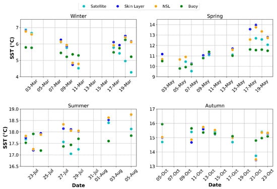
Figure 4.
Temperature ranges in the four different seasons for the satellite remotely sensed SST (<1 mm), skin layer (<1 mm), NSL (~1 m), and buoy (~1 m).
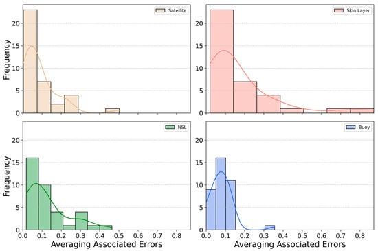
Figure 5.
Distribution of error associated with data averaging over time and space for the different data sources. Histograms represent the seven bins showing the error distribution, while the line shows the Kernel Density Estimation.
The box plot (Figure 6) shows the range of SST measurements across the observational platforms used. The satellite grid for the buoy location is not the same grid for HALOBATES, so we present the remotely sensed data as A and B for HALOBATES and buoy locations, respectively. This is because the mean of the remotely sensed data being compared with HALOBATES is different from that of the buoy due to the ASV taking up different positions each day instead of the fixed buoy data. The interquartile range (IQR), denoted by the grey box, contains the middle 50% of the data. The black line inside each box indicates the median SST value for that platform, with the limits representing the 25th and 75th percentiles. A primary finding of this study is that all platforms have similar ranges for SST data (Figure 6), indicating fairly consistent SST distributions with no statistically significant difference, as indicated by the Kruskal–Wallis test statistic of <0.38 and p-value of <0.83. The whiskers (extended lines from the box) represent the range of data within 1.5 times the IQR from the quartiles. The ends of the whiskers indicate the minimum and maximum values, excluding the outliers for each platform. It can be observed that the whiskers vary slightly, indicating some variation in SST values across sources, but this is not statistically significant, as Levene’s test revealed a statistic of <0.03 and a p-value of <0.98.
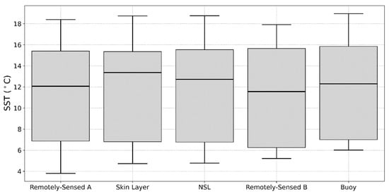
Figure 6.
SST distribution for the satellite remotely sensed data and HALOBATES (skin layer and NSL)-based datasets showing the median (black line in the box) and interquartile ranges. Whiskers (extended lines from the box) represent the range of data within 1.5 times the IQR from the quartiles. “Remotely Sensed A” is the satellite derived data at the location of HALOBATES, and B is at the location of the buoy.
Data from the flow-through CTDs were compared to those from the temperature probes, which were installed on the ladder of HALOBATEES for in situ measurements at various depths. For this comparison, a mean inter-sensor offset of 0.11 ± 0.11 °C was observed across the four campaigns. The CTD sensors showed warmer temperatures, ranging from 0.01 to 0.34 °C, compared to the temperature probes. This observed difference can be mainly attributed to the difference in measurement techniques, as the temperature probe is in direct contact with the water layer of interest, and the CTD relies on a flow-through system. The bias between the two sensor types fluctuated with seasons. We observed the lowest bias of –0.01 ± 0.07 °C during autumn and the highest bias of 0.20 ± 0.09 °C during spring. The biases for the winter and summer periods were 0.12 ± 0.12 °C and 0.10 ± 0.09 °C, respectively. The differences observed between the two sensors at 30 cm and 100 cm followed a normal distribution. Therefore, an independent t-test was conducted to determine whether the difference observed at 30 cm was statistically significant compared to that at 1 m. The t-test result (t-statistic = –0.12, p-value = 0.90) revealed that the observed biases at 30 cm depth were not statistically significant compared to the biases at 1 m depth. This shows that the flow-through system bias is consistent across depths. Figure 7 shows the distribution of these differences at 30 cm and 1 m (NSL) depths for the different seasons.
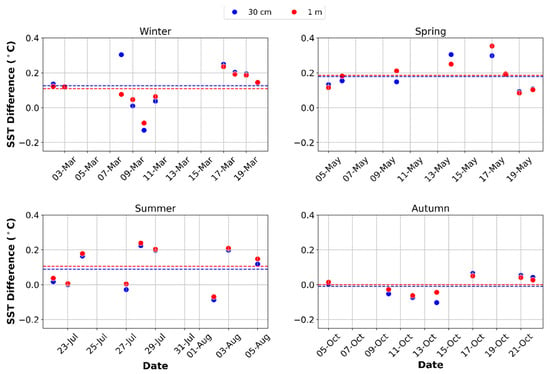
Figure 7.
Temperature differences between the CTDs and the temperature probes across the different seasons for the study period. Dashed lines are the mean difference at 30 cm (blue) and 1 m (red).
3.2. Results of Match-Up Analysis
For the match-up analysis, we used two approaches (i) to test the level of relationship between the datasets and (ii) to understand the nature of the difference between the datasets. First, we tested the presence and strength of the correlation between the datasets. The correlation of the remotely sensed SST with all in situ datasets showed correlation coefficients greater than 0.97 and p-values < 0.0001. The remotely sensed SST correlated with the skin layer and the NSL, demonstrating correlation coefficients of 0.98 for each, with a 95% confidence interval (CI) of 0.97 to 0.99. The correlation between the remotely sensed data and buoy data was 0.98, with a CI of 0.96 to 099 (Figure 8). This indicates that the remotely sensed SST accurately captures the changes in the in situ temperature over time.
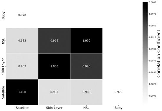
Figure 8.
Correlation matrix showing the correlation coefficients between the in situ and remotely sensed SST data. There was just a single measurement with HALOBATES close to the buoy, so these are not compared and are blanked out.
We further examined the nature of relationships between the remotely sensed data and the three in situ datasets using Deming regression. We observed a near one-to-one slope between the datasets. The buoy had a slightly higher slope of 0.99, with a CI of 0.97 to 1.02, while the NSL and skin layer had slopes and CIs of 0.94 to 1.02 and 0.92 to 1.01, respectively (Figure 9). The measurements from HALOBATES (skin layer and NSL) tend to have a relationship with a slope near to unity at higher SSTs compared to lower SSTs (Figure 9). However, the SST from the buoy maintains a stable slope, irrespective of the temperature range (Figure 9). We also observed that the remotely sensed SST tends to underestimate the in situ-derived SST, with intercepts of 0.84 °C, 0.66 °C, and 0.71 °C for the skin layer, NSL, and buoy SST, respectively. The associated coefficients of determination (R2) were all greater than 0.98, confirming the strong relationship between the remotely sensed SST and in situ measurements.
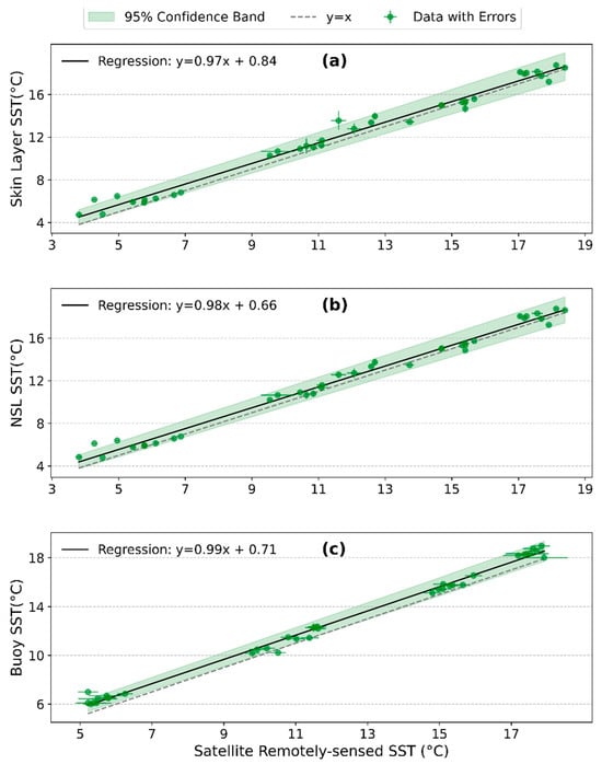
Figure 9.
Deming regression plot showing the relationship between the different in situ data and the remotely sensed SST: skin layer (a), NSL (b), and buoy (c). The black solid line is the Deming regression fit, which factors in the errors in both variables. The dashed grey line is the reference line if the two variables have a perfect 1:1 fit. The green band is the 95% confidence interval of the slope.
In the second approach, we further analysed these underestimations of SST in the remotely sensed SST, and a similar range (remotely sensed—in situ) of 2 °C was observed in all four seasons (Figure 10). These were predominantly negative differences, highlighting the warmer in situ measurements compared to the remotely sensed SST. However, we observed the largest positive differences on three days (10 October, 21 October, and 23 July) when the remotely sensed SST was at least 0.2 °C more than the in situ measurement (Figure 11). All three of these observations were made on rainy days.
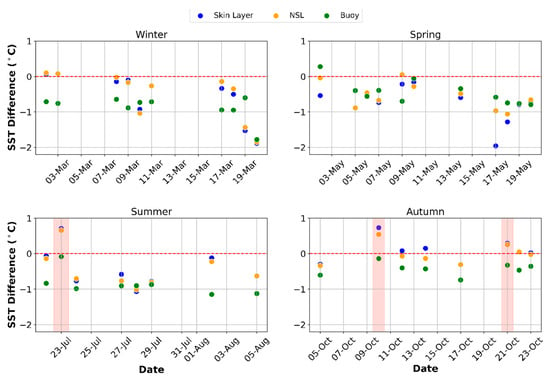
Figure 10.
Difference between remotely sensed SST and in situ SST (remotely sensed SST—in situ SST) across the seasons. Red dashed lines are the zero lines at which there is no difference between the remotely sensed SST and in situ. Negative SST difference on the y-axis indicates warmer in situ measurements and vice versa. Shaded red zones are days where remotely sensed SST—in situ SST > 0.2 °C.

Figure 11.
Temperature difference between the in situ and remotely sensed SST within a 95% confidence interval range (dashed green lines). Skin layer (a), NSL (b), and buoy (c), with mean temperature difference (dashed red line). “Average Temperature” is the average of the remotely sensed and in situ measurement being considered, whilst “Temperature Difference” is the difference between the two associated with each mean.
In comparison with the data obtained by the HALOBATES, the mean temperature difference between the remotely sensed and in situ SST was lower for the NSL and had a lower variability (–0.40 ± 0.52 °C) (Table 1) than the skin layer (–0.44 ± 0.60 °C). The buoy data had the highest mean difference and the least variability (–0.65 ± 0.35 °C). The one-way ANOVA test results showed no statistically significant difference in the SST between the remotely sensed and in situ data platforms, with a p-value of 0.90 and an F-statistic of 0.10. In addition, the difference between the platforms was not dependent on the prevailing temperature (Figure 11). An RMSE of 0.75 °C was obtained when the remotely sensed SST was compared with the skin layer, which decreased to 0.66 °C for the NSL. The buoy temperature data at a depth of 1 m had an RMSE of 0.74 °C.

Table 1.
Summary of statistics for the various in situ platforms compared to the remotely sensed SST. The mean and its associated error, “Standard Deviation of Mean Bias”, shows widespread bias between remotely sensed SST and in situ data. The skin layer and NSL measured with the HALOBATES and a 1 m depth measurement from the buoy.
4. Discussion
A rigorous correction of the intra-sensor offset between the CTD sensors makes the measurement more reliable. This was performed to ensure that the biases we report between the remotely sensed SST and HALOBATES measurements for the skin layer and NSL did not arise from the intra-sensor offset of the CTDs measuring different depths. We also evaluated our flow method via the CTDs against direct contact measurements with the temperature probes. We observed a bias of 0.11 ± 0.11 °C between the CTDs and temperature probes, and this likely originates from the fact that the probes are in direct contact with the water, while the CTDs are not. The CTDs rely on a peristaltic pump, which can cause some level of warming of the water being pumped over time, and a flow-throw system with tubes partially (<4% of the total length) exposed to sunlight and warming.
The difference between the CTDs and temperature probes is not used in correcting the CTD temperatures but is reported as a possible source of bias. Another reason for not using the difference to correct the data was the good agreement we observed between the measurements in the skin layer via the combined glass disc sampling with a flow-through system and remote sensing via an infrared camera [30], based on observations with our earlier radio-controlled surface vehicle model [19]. Additionally, the bias in our study between the two was neither consistent nor directly correlated to the seasonal cycle, ranging from –0.17 to 0.29 °C. This highlights that prevailing temperatures did not drive the observed bias as we moved from colder to warmer seasons and vice versa.
The coefficient of determination (R2) revealed that more than 98% of the variability in remotely sensed SST is explained by in situ observations. This suggests that in situ observations explain nearly all the variability in remotely sensed SST, with less than 2% attributed to other factors. The remotely sensed data captured the changes in the in situ data, as shown by the strong correlation coefficient (r) > 0.98. This shows a strong linear relationship between the remotely sensed and in situ SST. In other words, with a 1 °C increase in remotely sensed SST, the corresponding in situ temperature increases by 0.98 °C. Most of the literature reported that the R2 and correlation coefficients (r) across different seas are less than 98% and 0.98, respectively, highlighting the robustness of our measurements [11,13,16].
Similar values of R2 = 0.95–0.97 and r > 0.96 were reported by Brewin et al. [13] at a depth of approximately 1 m offshore Plymouth, UK. Gomez et al. [11] reported 0.91 < r > 0.96 for coral reef zones at depths of approximately 1 m in the Caribbean Sea. Other studies have reported 0.64 > r < 0.88 [16], but this may be attributed to the coastal nature of the zone and the difficulty in retrieving satellite-derived SST due to land contamination. However, we observed a 1% increase in R2 for the measurement from the NSL and buoy compared to the skin layer, which may be attributed to the diurnal warming affecting the skin layer to the highest degree [31] and other localised, small-scale processes due to air–sea interactions. However, the strong correlation makes the investigated satellite product suitable for studying fluctuations and temporal trends of the sea-surface, that is, ranging from the skin layer to the 1 m NSL.
Nonetheless, the overall observed mean bias (−0.42 ± 0.56 °C) shows that the remotely sensed SST has a cold bias compared to the in situ measurements. A possible reason for the cold bias is the effect of cloud cover on the retrieval of satellite-derived SST [32,33]. The measured radiance is a combination of emissions from the sea surface and the cloud tops, and correcting for the cloud effect can create these biases. Additionally, undetected clouds, due to their total number or the efficacy of the detection algorithm, lead to negative bias tendencies [34]. This cold bias (up to −1 °C) has been observed in other areas, such as offshore of the Korean Peninsula [10], the South African coast [35], and in the Gulf of Honduras [36]. We also hypothesise that another possible reason for this cold bias might be the derivation of the daytime remotely sensed SST from the nighttime SST. This is because the different radiometers onboard the satellites used in the product integrate both day- and nighttime measurements. In the absence of daytime measurements as used by the data providers, inferences will be made from the colder nighttime measurements. The quality information document for the satellite dataset [26] revealed stronger cold biases during the day (−0.20 °C) compared to the night (−0.14 °C). We noted a shift to warmer biases on three rainy days, and this can be as a result of the rain being colder than the SST, causing a cooling (Gassen et al., 2024 [37]). The rain was in patches, so sometimes we could be in a rain front, but we can physically see another area where it is not raining. The rain creates a cooling effect that we capture, but the satellite data may not account for it due to the data being generated from a different overpass time.
Our studies revealed an RMSE of ~0.71 °C, which shows that, on average, the remotely sensed SST deviates by 0.71 °C from the in situ SST. The mean bias and RMSE agree with most findings for various validation approaches of satellite-derived SST, usually between 0.3 and 1.5 °C [10,11,12,13,14,15,16,34] for various seas and regions in the global ocean. The buoy data had higher biases but less variability (mean bias = −0.66 ± 0.35 °C, RMSE = 0.75) compared to the NSL from the ASV (mean bias = −0.40 ± 0.52 °C, RMSE = 0.66), even though the buoy data represent SST measurements from the same depth as the ASV’s NSL (1 m).
This may be due to the proximity of the buoy to the Helgoland island (~800 m), as satellite data retrieval within such zones can be challenging compared with the open ocean [38,39]. In addition, the lower variability could be attributed to the fixed position of the buoy, which limits the spatial variability to a narrow radius. In addition, other studies have noted higher mean biases in the BSH buoys in the North Sea [14]. The relatively small disparity between the skin layer and NSL from the ASV highlights that the satellite remotely sensed SST data tend to be better suited to the NSL than the dynamic skin layer (~0.1 °C in RMSE). The skin layer also showed more variability in the observed mean bias than the NSL, representing highly dynamic surface processes at the top few millimetres of the ocean [3], such as heat flux, evaporation, and wind stress.
The ocean state can have an impact on the obtained data due to the measurement technique. Wavy conditions lead to heaving, rolling, pitching, and possible splashing. To reduce these effects, we opt for a drifting mode instead of automated missions. The drifting mode allows the ASV to passively float with the current and winds rather than fighting waves and amplifying motion effects. Additionally, the glass disc assembly is covered with a semi-transparent acrylic glass hood with ventilation slits [18]. This helps avoid splashing but also creates room for ventilation to avoid evaporative cooling. Wave-induced uncertainties are also introduced due to their impact on surface layers, as turbulence can lead to a degree of mixing. The temporal and spatial relationship between the skin and NSLs is highly variable under low-wind conditions [1]. Diurnal heating also creates a difference between the skin and NSL [40], and this depends on a number of factors including the season, solar radiation, and cloud cover over the area.
5. Conclusions
We provide over 225 h of ocean skin and NSL data for comparisons with remotely sensed SST. We assessed the robustness of our measurement via the flow-through system by comparing and revealing its bias to submerged temperature probes. The bias between our two systems was approximately four times less than the bias between our flow-through system and remotely sensed SST. Furthermore, based on the observed correlations, we can conclude that the use of remotely sensed SST is suitable for studying the dynamic processes and trends of the North Sea. However, the current remotely sensed SST levels in the North Sea are most likely understated due to the observed cold bias. It must also be emphasised that the remotely sensed SST tends to match-up slightly better when compared to the in situ NSL as opposed to the skin layer. Moreover, the dynamic nature of the skin layer, influenced by rapid surface processes, results in more variability than the NSL based on the observed deviations associated with the mean bias. The comparative analysis of the 1-m depth from the buoy and ASV datasets revealed that the ASV’s measurements were better aligned with the satellite-derived SST.
These findings contribute to a broader understanding of SST measurement accuracy, emphasising the utility of satellite-derived SSTs in both scientific research and operational applications. Nonetheless, future work should focus on exploring the impacts of the depth-wise scaling of data from the NSL through deep learning approaches, such as neural networks and mathematical models, to approximate the skin layer temperature due to the difficulty in obtaining extensive in situ data for the skin layer. The advancement of retrieval and correction algorithms to account for small-scale processes that influence the skin and NSL temperature dynamics would help curb the observed cold bias. Thus, we affirm the need for continuous investments in satellite and in situ monitoring systems, as they complement each other in providing comprehensive data to support early warning systems and climate change adaptation.
Author Contributions
Conceptualization, O.W. and M.R.-R.; methodology, S.M.A. and O.W.; formal analysis, S.M.A.; investigation, S.M.A., L.G. and O.W.; data curation, S.M.A. and L.G.; writing—original draft preparation, S.M.A.; writing—review and editing, L.G., M.R.-R. and O.W.; visualisation, S.M.A.; supervision, O.W.; project administration, O.W.; funding acquisition, O.W. All authors have read and agreed to the published version of the manuscript.
Funding
This research (“The North Sea from Space: Using Explainable Artificial Intelligence to Improve Satellite Observations of Climate Change (NorthSat-X)”) was funded by the Lower Saxony Ministry of Science and Culture, grant number VWZN3680.
Data Availability Statement
All data are freely available at the data repository PANGAEA as follows. Digital object identifiers are available for processed data from the HALOBATES. HE598; https://doi.pangaea.de/10.1594/PANGAEA.968799, accessed on 25 September 2025. HE609; https://doi.pangaea.de/10.1594/PANGAEA.968800, accessed on 25 September 2025. HE614; https://doi.pangaea.de/10.1594/PANGAEA.969378, accessed on 25 September 2025. HE626; https://doi.pangaea.de/10.1594/PANGAEA.972989, accessed on 25 September 2025. Satellite data; https://doi.org/10.48670/moi-00309, accessed on 28 November 2023. Buoy data; https://doi.org/10.48670/moi-00036, accessed on 19 December 2023 via repository link https://data-marineinsitu.ifremer.fr/glo_multiparameter_nrt/history/MO/, accessed on 19 December 2025.
Acknowledgments
We thank the Lower Saxony Ministry of Science and Culture (MWK) for funding this project. We also thank the German Research foundation (DFG) for funding the SCANS cruises on the RV Heincke. We thank the crew and ship coordination of the RV Heincke for helping with the operations of HALOBATES during the missions, including deployment and recovery. We thank colleagues in our workshop for the maintenance of the mechanical structures of HALOBATES. We are also grateful to the science team on the RV Heincke for their support in the deployment and recovery of HALOBATES.
Conflicts of Interest
The authors declare no conflicts of interest. The funders had no role in the design of the study; in the collection, analyses, or interpretation of data; in the writing of the manuscript; or in the decision to publish the results.
Abbreviations
The following abbreviations were used in the manuscript:
| ANOVA | Analysis of Variance |
| ASV | Autonomous Surface Vehicle |
| AVHRR | Advanced Very-High-Resolution Radiometer |
| BSH | German Federal Maritime and Hydrographic Agency |
| CI | Confidence Interval |
| CTD | Conductivity, Temperature, and Depth Sensor |
| IQR | Interquartile Range |
| MSG | Meteosat Second Generation |
| NSL | Near-Surface Layer (1 m depth) |
| RMSE | Root-Mean-Square Error |
| RV | Research Vessel |
| SST | Sea Surface Temperature |
| SEVIRI | Spinning Enhanced Visible and Infrared Imager |
| SLSTR | Sea and Land Surface Temperature Radiometer |
| Suomi NPP | National Polar-Orbiting Partnership |
References
- Donlon, C.J.; Minnett, P.J.; Gentemann, C.; Nightingale, T.J.; Barton, I.J.; Ward, B.; Murray, M.J. Toward Improved Validation of Satellite Sea Surface Skin Temperature Measurements for Climate Research. J. Clim. 2002, 15, 353–369. [Google Scholar] [CrossRef]
- Dong, Y.; Bakker, D.C.E.; Bell, T.G.; Huang, B.; Landschützer, P.; Liss, P.S.; Yang, M. Update on the Temperature Corrections of Global Air-Sea CO2 Flux Estimates. Glob. Biogeochem. Cycles 2022, 36, e2022GB007360. [Google Scholar] [CrossRef]
- Fairall, C.W.; Bradley, E.F.; Hare, J.E.; Grachev, A.A.; Edson, J.B. Bulk Parameterization of Air–Sea Fluxes: Updates and Verification for the COARE Algorithm. J. Clim. 2003, 16, 571–591. [Google Scholar] [CrossRef]
- Castro, S.L.; Wick, G.A.; Steele, M. Validation of Satellite Sea Surface Temperature Analyses in the Beaufort Sea Using UpTempO Buoys. Remote Sens. Environ. 2016, 187, 458–475. [Google Scholar] [CrossRef]
- Yu, W.; Ma, M. Scale Mismatch Between In Situ and Remote Sensing Observations of Land Surface Temperature: Implications for the Validation of Remote Sensing LST Products. IEEE Geosci. Remote Sens. Lett. 2014, 12, 497–501. [Google Scholar] [CrossRef]
- Ribas-Ribas, M.; Zappa, C.; Wurl, O. Technologies for Observing the Near Sea Surface. Oceanography 2021, 34, 88–89. [Google Scholar] [CrossRef]
- Wurl, O.; Ekau, W.; Landing, W.M.; Zappa, C.J. Sea Surface Microlayer in a Changing Ocean—A Perspective. Elem. Sci. Anthr. 2017, 5, 31. [Google Scholar] [CrossRef]
- Pearson, K.; Merchant, C.; Embury, O.; Donlon, C. The Role of Advanced Microwave Scanning Radiometer 2 Channels within an Optimal Estimation Scheme for Sea Surface Temperature. Remote Sens. 2018, 10, 90. [Google Scholar] [CrossRef]
- Lee, M.-A.; Chang, Y.; Sakaida, F.; Kawamura, H.; Cheng, C.-H.; Chan, J.-W.; Huang, I. Validation of Satellite-Derived Sea Surface Temperatures for Waters around Taiwan. Terr. Atmos. Ocean. Sci. 2005, 16, 1189. [Google Scholar] [CrossRef]
- Kwak, M.-T.; Seo, G.-H.; Cho, Y.-K.; Kim, B.-G.; You, S.H.; Seo, J.-W. Long-Term Comparison of Satellite and in-Situ Sea Surface Temperatures around the Korean Peninsula. Ocean Sci. J. 2015, 50, 109–117. [Google Scholar] [CrossRef]
- Gomez, A.M.; McDonald, K.C.; Shein, K.; DeVries, S.; Armstrong, R.A.; Hernandez, W.J.; Carlo, M. Comparison of Satellite-Based Sea Surface Temperature to In Situ Observations Surrounding Coral Reefs in La Parguera, Puerto Rico. J. Mar. Sci. Eng. 2020, 8, 453. [Google Scholar] [CrossRef]
- Wu, Y. A Comparative Study of Satellite-Based Operational Analyses and Ship-Based in-Situ Observations of Sea Surface Temperatures over the Eastern Canadian Shelf. Satell. Oceanogr. Meteorol. 2023, 1, 29–38. [Google Scholar] [CrossRef]
- Brewin, R.; Smale, D.; Moore, P.; Dall’Olmo, G.; Miller, P.; Taylor, B.; Smyth, T.; Fishwick, J.; Yang, M. Evaluating Operational AVHRR Sea Surface Temperature Data at the Coastline Using Benthic Temperature Loggers. Remote Sens. 2018, 10, 925. [Google Scholar] [CrossRef]
- Høyer, J.L.; She, J. Optimal Interpolation of Sea Surface Temperature for the North Sea and Baltic Sea. J. Mar. Syst. 2007, 65, 176–189. [Google Scholar] [CrossRef]
- Høyer, J.L.; Le Borgne, P.; Eastwood, S. A Bias Correction Method for Arctic Satellite Sea Surface Temperature Observations. Remote Sens. Environ. 2014, 146, 201–213. [Google Scholar] [CrossRef]
- Thakur, K.K.; Vanderstichel, R.; Barrell, J.; Stryhn, H.; Patanasatienkul, T.; Revie, C.W. Comparison of Remotely-Sensed Sea Surface Temperature and Salinity Products With in Situ Measurements From British Columbia, Canada. Front. Mar. Sci. 2018, 5, 121. [Google Scholar] [CrossRef]
- Li, Z.; Wu, H.; Duan, S.; Zhao, W.; Ren, H.; Liu, X.; Leng, P.; Tang, R.; Ye, X.; Zhu, J.; et al. Satellite Remote Sensing of Global Land Surface Temperature: Definition, Methods, Products, and Applications. Rev. Geophys. 2023, 61, e2022RG000777. [Google Scholar] [CrossRef]
- Wurl, O.; Gassen, L.; Badewien, T.H.; Braun, A.; Emig, S.; Holthusen, L.A.; Lehners, C.; Meyerjürgens, J.; Ribas, M.R. HALOBATES: An Autonomous Surface Vehicle for High-Resolution Mapping of the Sea-Surface Microlayer and near-Surface Layer on Essential Climate Variables. J. Atmos. Ocean. Technol. 2024, 41, 1197–1211. [Google Scholar] [CrossRef]
- Ribas-Ribas, M.; Hamizah Mustaffa, N.I.; Rahlff, J.; Stolle, C.; Wurl, O. Sea Surface Scanner (S3): A Catamaran for High-Resolution Measurements of Biogeochemical Properties of the Sea Surface Microlayer. J. Atmos. Ocean. Technol. 2017, 34, 1433–1448. [Google Scholar] [CrossRef]
- Shinki, M.; Wendeberg, M.; Vagle, S.; Cullen, J.T.; Hore, D.K. Characterization of Adsorbed Microlayer Thickness on an Oceanic Glass Plate Sampler. Limnol. Ocean Methods 2012, 10, 728–735. [Google Scholar] [CrossRef]
- Horrocks, L.A.; Candy, B.; Nightingale, T.J.; Saunders, R.W.; O’Carroll, A.; Harris, A.R. Parameterizations of the Ocean Skin Effect and Implications for Satellite-based Measurement of Sea-surface Temperature. J. Geophys. Res. 2003, 108, 2002JC001503. [Google Scholar] [CrossRef]
- Ayim, S.M.; Bibi, R.; Cortés, E.; Gassen, L.; Jaeger, L.; Lehners, C.; Ribas-Ribas, M.; Wurl, O. High-Resolution Measurements of Essential Climate Variables in the North Sea from the Autonomous Surface Vehicle HALOBATES During RV Heincke Cruise HE626 [Dataset]. PANGAEA. 2025. Available online: https://doi.pangaea.de/10.1594/PANGAEA.972989 (accessed on 25 September 2025).
- Gassen, L.; Ayim, S.M.; Bibi, R.; Cortés, E.; Holthusen, L.A.; Jaeger, L.; Lagemann, M.; Lehners, C.; Ribas-Ribas, M.; Wurl, O. High-Resolution Measurements of Essential Climate Variables in the North Sea from the Autonomous Surface Vehicle HALOBATES During RV Heincke Cruise HE614 2024, 1368766 Data Points. PANGAEA. 2024. Available online: https://doi.pangaea.de/10.1594/PANGAEA.969378 (accessed on 25 September 2025).
- Gassen, L.; Ayim, S.M.; Emig, S.; Goßmann, I.; Holthusen, L.A.; Jaeger, L.; Lagemann, M.; Lehners, C.; Ribas-Ribas, M.; Wurl, O. High-Resolution Measurements of Essential Climate Variables in the North Sea from the Autonomous Surface Vehicle HALOBATES During RV Heincke Cruise HE598 2024, 1019068 Data Points. PANGAEA. 2024. Available online: https://doi.pangaea.de/10.1594/PANGAEA.968799 (accessed on 25 September 2025).
- Gassen, L.; Ayim, S.M.; Emig, S.; Holthusen, L.A.; Jaeger, L.; Lagemann, M.; Lehners, C.; Ribas-Ribas, M.; Wurl, O. High-Resolution Measurements of Essential Climate Variables in the North Sea from the Autonomous Surface Vehicle HALOBATES During RV Heincke Cruise HE609 2025. PANGAEA. 2025. Available online: https://doi.pangaea.de/10.1594/PANGAEA.968800 (accessed on 25 September 2025).
- European Union-Copernicus Marine Service. Baltic Sea—Diurnal Subskin Sea Surface Temperature Analysis. 2022. Available online: https://data.marine.copernicus.eu/product/SST_BAL_PHY_SUBSKIN_L4_NRT_010_034/description (accessed on 28 November 2023).
- Merchant, C.J.; Embury, O.; Bulgin, C.E.; Block, T.; Corlett, G.K.; Fiedler, E.; Good, S.A.; Mittaz, J.; Rayner, N.A.; Berry, D.; et al. Satellite-Based Time-Series of Sea-Surface Temperature since 1981 for Climate Applications. Sci. Data 2019, 6, 223. [Google Scholar] [CrossRef]
- Vinogradova, N.T.; Ponte, R.M. Small-Scale Variability in Sea Surface Salinity and Implications for Satellite-Derived Measurements. J. Atmos. Ocean. Technol. 2013, 30, 2689–2694. [Google Scholar] [CrossRef]
- Jessup, A.T.; Branch, R. Integrated Ocean Skin and Bulk Temperature Measurements Using the Calibrated Infrared In Situ Measurement System (CIRIMS) and Through-Hull Ports. J. Atmos. Ocean. Technol. 2008, 25, 579–597. [Google Scholar] [CrossRef]
- Wurl, O.; Landing, W.M.; Mustaffa, N.I.H.; Ribas-Ribas, M.; Witte, C.R.; Zappa, C.J. The Ocean’s Skin Layer in the Tropics. J. Geophys. Res. Ocean. 2019, 124, 59–74. [Google Scholar] [CrossRef] [PubMed]
- Donlon, C.; Robinson, I.; Casey, K.S.; Vazquez-Cuervo, J.; Armstrong, E.; Arino, O.; Gentemann, C.; May, D.; LeBorgne, P.; Piollé, J.; et al. The Global Ocean Data Assimilation Experiment High-Resolution Sea Surface Temperature Pilot Project. Bull. Am. Meteorol. Soc. 2007, 88, 1197–1214. [Google Scholar] [CrossRef]
- Casey, K.S.; Cornillon, P. A Comparison of Satellite and In Situ–Based Sea Surface Temperature Climatologies. J. Clim. 1999, 12, 1848–1863. [Google Scholar] [CrossRef]
- Minnett, P.J.; Alvera-Azcárate, A.; Chin, T.M.; Corlett, G.K.; Gentemann, C.L.; Karagali, I.; Li, X.; Marsouin, A.; Marullo, S.; Maturi, E.; et al. Half a Century of Satellite Remote Sensing of Sea-Surface Temperature. Remote Sens. Environ. 2019, 233, 111366. [Google Scholar] [CrossRef]
- Wick, G.A.; Bates, J.J.; Scott, D.J. Satellite and Skin-Layer Effects on the Accuracy of Sea Surface Temperature Measurements from the GOES Satellites. J. Atmos. Ocean. Technol. 2002, 19, 1834–1848. [Google Scholar] [CrossRef]
- Smit, A.J.; Roberts, M.; Anderson, R.J.; Dufois, F.; Dudley, S.F.J.; Bornman, T.G.; Olbers, J.; Bolton, J.J. A Coastal Seawater Temperature Dataset for Biogeographical Studies: Large Biases between In Situ and Remotely-Sensed Data Sets around the Coast of South Africa. PLoS ONE 2013, 8, e81944. [Google Scholar] [CrossRef]
- Castillo, K.D.; Lima, F.P. Comparison of in Situ and Satellite-derived (MODIS-Aqua/Terra) Methods for Assessing Temperatures on Coral Reefs. Limnol. Ocean Methods 2010, 8, 107–117. [Google Scholar] [CrossRef]
- Gassen, L.; Ayim, S.M.; Badewien, T.H.; Ribas-Ribas, M.; Wurl, O. Wind Speed Effects on Rainfall-Induced Salinity and Temperature Anomalies at the Sea Surface Microlayer at Mid-Latitudes. Elem. Sci. Anth. 2024, 12, 00004. [Google Scholar] [CrossRef]
- Dash, P.; Ignatov, A.; Martin, M.; Donlon, C.; Brasnett, B.; Reynolds, R.W.; Banzon, V.; Beggs, H.; Cayula, J.-F.; Chao, Y.; et al. Group for High Resolution Sea Surface Temperature (GHRSST) Analysis Fields Inter-Comparisons—Part 2: Near Real Time Web-Based Level 4 SST Quality Monitor (L4-SQUAM). Deep Sea Res. Part II Top. Stud. Oceanogr. 2012, 77–80, 31–43. [Google Scholar] [CrossRef]
- Donlon, C.; Berruti, B.; Buongiorno, A.; Ferreira, M.-H.; Féménias, P.; Frerick, J.; Goryl, P.; Klein, U.; Laur, H.; Mavrocordatos, C.; et al. The Global Monitoring for Environment and Security (GMES) Sentinel-3 Mission. Remote Sens. Environ. 2012, 120, 37–57. [Google Scholar] [CrossRef]
- Kilpatrick, K.A.; Podestá, G.; Walsh, S.; Williams, E.; Halliwell, V.; Szczodrak, M.; Brown, O.B.; Minnett, P.J.; Evans, R. A Decade of Sea Surface Temperature from MODIS. Remote Sens. Environ. 2015, 165, 27–41. [Google Scholar] [CrossRef]
Disclaimer/Publisher’s Note: The statements, opinions and data contained in all publications are solely those of the individual author(s) and contributor(s) and not of MDPI and/or the editor(s). MDPI and/or the editor(s) disclaim responsibility for any injury to people or property resulting from any ideas, methods, instructions or products referred to in the content. |
© 2025 by the authors. Licensee MDPI, Basel, Switzerland. This article is an open access article distributed under the terms and conditions of the Creative Commons Attribution (CC BY) license (https://creativecommons.org/licenses/by/4.0/).