Variation Characteristics of the Ionospheric E Layer over the Tibetan Plateau and Surrounding Areas During a Full Solar Cycle

Highlights

What is the main finding?

• The diurnal and seasonal inconsistencies in the spatial distribution of the critical frequency of the ionospheric E layer over the Tibetan Plateau and its surrounding areas have been discovered for the first time.

What is the implication of the main finding?

• The discovery of the diurnal and seasonal inconsistencies of the ionospheric E layer over the Tibetan Plateau areas is of great significance for revealing the mechanisms of atmosphere coupling.

Abstract

The ionospheric E layer (90–150 km altitude) significantly influences ionospheric dynamics and plays a crucial role in radio wave propagation. The Tibetan Plateau, as the “Third Pole,” affects E-layer morphology due to its unique topographical factors. Given the limited systematic studies in this high-altitude region, this study analyzes E-layer spatiotemporal characteristics and their controlling mechanisms over the Tibetan Plateau and adjacent regions. We analyzed foE (critical frequency of E-layer) data from six ionospheric observation stations across the Tibetan Plateau and neighboring areas during 2013–2023, covering a complete solar cycle from solar minimum to maximum. Combined with sunspot numbers as solar activity indicators, we systematically examined diurnal, seasonal, and solar cycle variations to understand regional E-layer behavior patterns. Daytime foE values significantly exceed nighttime values, demonstrating strong solar control. Spatially, Kunming shows the strongest daytime E-layer intensity with peak values reaching 3.12 MHz, while Urumqi exhibits the weakest at 2.94 MHz. Daytime foE values decrease with increasing latitude, whereas nighttime values show opposite latitudinal trends, indicating pronounced diurnal distribution asymmetry. Kunming displays the largest day-night foE variation amplitude, while Urumqi shows the smallest changes. Notably, most stations exhibit E-layer intensity peaks in July rather than June when solar zenith angles are minimum, differing from typical mid-low latitude seasonal behavior. These patterns may be related to complex vertical atmospheric coupling influenced by the region’s unique topography, which could affect the spatiotemporal distribution of the E-layer over the Tibetan Plateau.

1. Introduction

The ionospheric E layer is an essential component of the lower ionosphere, typically located at altitudes of about 90–150 km. It represents a typical photochemical equilibrium region in the upper atmosphere, where ionization is mainly driven by the photoionization of molecular oxygen under solar extreme ultraviolet (EUV) and soft X-ray radiation [1,2,3]. Under normal conditions, E-layer ionization is maintained primarily by solar radiation. As a result, electron density is significantly higher during the daytime and decreases sharply at night, sometimes nearly disappearing. This pronounced diurnal variation makes the E layer an important physical platform for studying solar–terrestrial coupling processes [4].

The regular E layer can reflect high-frequency (HF) and medium-frequency (MF) radio waves below the critical frequency, typically in the range of 1–10 MHz [5], and thus plays a vital role in long-distance communication such as maritime navigation and shortwave broadcasting [6]. In recent years, with the development of satellite-to-ground quantum key distribution (QKD) technology, increasing attention has been paid to the potential influence of the ionospheric environment on optical signal transmission. Although the E layer is essentially transparent to visible and near-infrared bands, the combined state of the atmosphere and ionosphere may still affect the stability of QKD links through turbulence, scattering, and absorption processes [7].

Early studies of the E layer in the twentieth century primarily focused on electron density measurements and the development of theoretical models for its formation. The vertical structure of the E layer is mainly described by the Chapman model [8], which is based on the balance between photoionization and recombination while considering the effects of solar zenith angle and solar radiation flux [8]. The critical frequency foE serves as a key parameter for evaluating the ionospheric photochemical equilibrium and testing model validity. In the classical Chapman theory, under isothermal and equilibrium assumptions, the E-layer electron density distribution can be described by a simplified atmospheric model, which further yields the relationship between foE and the solar zenith angle χ:

$$f_{O}E=9000{\left[\left({\displaystyle \frac{q_0}{\alpha }}\right)\mathit{cos}\chi \right]}^{0.25}\left(Hz\right)$$

(1)

where $q_0$ is the peak production rate at $\chi =0$ and $\alpha$ is the recombination coefficient. More generally, it can be expressed as:

$$f_{O}E=A(\mathit{cos}\chi {)}^{0.25}\left(Hz\right)$$

(2)

The parameter $A$ is associated with the ionization production and loss rates. Although this model has been widely applied in electron density simulation and frequency prediction [9,10], by the 1990s the simulated E-layer peak electron density was still generally underestimated. For example, NmE was typically lower than observations by about 30%, primarily due to incomplete physical processes, the absence of secondary ionization sources, and discrepancies between experimental settings and the real atmospheric environment. In recent years, improvements in observations and model parameterizations have reduced this deviation to approximately 10%. The International Reference Ionosphere (IRI) model has also adjusted the E-layer peak height to around 110 km to better match reality [11,12]. Nevertheless, actual observations often deviate from this idealized model, particularly in regions with complex terrain or irregular atmospheric structures. Such discrepancies highlight the necessity of conducting empirical studies in diverse geographic environments to enhance the applicability and accuracy of the model. Therefore, the acquisition of high-quality observational data is crucial.

Ionospheric observation techniques have evolved significantly, integrating ground-based and space-based platforms [13,14]. While space-based techniques such as radio occultation and LEO satellites offer broader spatial coverage and multi-platform data fusion has enhanced multi-scale studies [15], understanding long-term regional ionospheric behavior requires consistent, high-resolution temporal measurements at fixed locations over extended periods [16]. In this context, ionospheric vertical sounding (ionosonde) networks demonstrate unique value. Multi-station ionosonde systems provide continuous monitoring with high temporal resolution, deriving key parameters including critical frequency, electron density, and reflection height through signal echo analysis [17,18]. When coordinated across a region, multiple stations capture the spatial and temporal evolution of ionospheric phenomena, revealing diurnal, seasonal, and solar cycle dependencies critical for regional studies.

This multi-platform integration has not only enhanced the understanding of ionospheric features but also shifted the research perspective from a single-layer focus toward a coupled atmosphere–ionosphere system. Increasing evidence shows that the ionosphere interacts closely with the lower atmosphere, especially through vertical coupling mechanisms [19]. Such coupling effects are particularly pronounced in regions with complex topography, such as the Tibetan Plateau—the largest plateau on Earth—which plays a crucial role in both atmospheric circulation and ionospheric variability. Due to its unique geomorphological characteristics and atmosphere–ionosphere coupling effects, the ionosphere over the Tibetan Plateau exhibits significant spatial inhomogeneity and dynamic variability [20]. Against this background, the role of the E layer is especially important: it acts both as a direct responder to solar forcing and as an active participant in atmosphere–ionosphere coupling.

Based on this, many recent studies have focused on improving empirical and theoretical models of the E layer, particularly at low and middle latitudes. Data from the Chinese ionosonde network have become a crucial source for refining E-layer models, leading to the development of several empirical models [21,22,23,24,25,26]. Although these studies have greatly advanced the understanding of E-layer behavior under various space weather conditions, most of them focus on typical latitude bands and relatively homogeneous terrains [27]. Meanwhile, the IRI model, widely used as an empirical reference ionospheric model, incorporates little data from China, and its applicability to this region remains uncertain [28]. Therefore, the behavior of the E layer in geographically complex areas such as the Tibetan Plateau requires further investigation.

This study aims to investigate the unique spatiotemporal evolution of the E-layer critical frequency (foE) over the Tibetan Plateau by analyzing long-term observations covering a complete solar cycle. Using multi-station ionosonde data from six sites (Urumqi, Lanzhou, Xi’an, Lhasa, Kunming, and Chongqing), this study examines diurnal and seasonal variations, as well as solar-cycle responses, of the regional E layer. Differences from conventional models are also analyzed. By integrating multi-station data through spatial interpolation, this work provides new insights into atmosphere–ionosphere vertical coupling, while supporting regional ionospheric modeling, radio propagation prediction, and space weather monitoring.

2. Data Sources and Methods

This study draws upon continuous ionospheric observations from six ionosonde stations situated in and around the Tibetan Plateau—specifically, Chongqing, Lanzhou, Lhasa, Kunming, Xi’an, and Urumqi—covering an eleven-year period from 2013 to 2023. The geographic coordinates, altitude, and data collection period of each station are listed in Table 1, and their spatial distribution is shown in Figure 1. The data were provided by the China Research Institute of Radiowave Propagation. The ionograms data employed in this study were manually scaled, with a temporal resolution of 1 h.

Table 1. Observation stations and corresponding data coverage periods.

No.	Station	Latitude (°N)	Longitude (°E)	Observation Period	Altitude (m)
1	Urumqi	43.7	87.6	2013–2023	873
2	Lanzhou	36.1	103.7	2013–2023	1528
3	Xi’an	34.2	108.9	2013–2023	405
4	Lhasa	29.6	91.1	2013–2023	3657
5	Chongqing	29.5	106.5	2013–2023	266
6	Kunming	25.2	102.7	2013–2023	1906

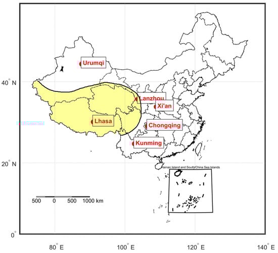
Figure 1. Geographical distribution of the selected ionosonde stations over and around the Tibetan Plateau.

The six selected ionosonde stations span a wide range of geographical locations across the Tibetan Plateau and its surrounding regions, encompassing the plateau’s interior (Lhasa), eastern margin (Xi’an and Lanzhou), southern edge (Kunming), northern edge (Urumqi), and southeastern foothills (Chongqing). This strategically distributed network ensures broad spatial coverage, enabling a more comprehensive assessment of the E-layer structure and dynamics over both the core and peripheral regions of the Tibetan Plateau.

Given the Plateau’s unique and highly variable topography, which significantly influences ionospheric processes, the spatial diversity of these stations supports the identification of regional variations in E-layer behavior. Each station is subject to distinct ionospheric driving forces—such as solar radiation intensity, geomagnetic field configuration, and atmospheric wave activity—allowing for comparative analysis to distinguish between local anomalies and large-scale ionospheric patterns.

The dataset covers a complete solar cycle, and all temporal data presented in this study are expressed in local time, making it particularly suitable for examining diurnal, seasonal, and interannual variations in the E-layer. It also provides a valuable foundation for exploring how solar activity, geomagnetic disturbances, and lower atmospheric forcing jointly modulate E-layer characteristics over this complex high-altitude region.

The critical frequency of the ionospheric E layer (foE), obtained from ionograms, is a fundamental parameter measured by ionosondes and serves as a key indicator of the E-layer’s electron density and overall strength. In this section, we utilize foE data from six ionosonde stations—Urumqi, Lanzhou, Xi’an, Lhasa, Kunming, and Chongqing—operated within the Chinese ionospheric sounding network and located in and around the Tibetan Plateau, to perform a comprehensive analysis of the E-layer characteristics in this region. The analysis covers aspects including intensity, spatial distribution, diurnal and seasonal variations, as well as long-term trends. These results offer important insights into the spatiotemporal variability of the ionospheric E layer and enhance our understanding of the coupling mechanisms between the ionosphere and the lower atmosphere.

The identification and interpretation of ionospheric E layer versus sporadic E layer primarily rely on distinct ionogram trace morphologies: E-layer traces manifest as smooth parabolic curves, whereas Es-layer traces appear as continuous or fragmented horizontal lines. It should be noted that the occurrence probability of the regular E-layer during certain nighttime periods at some stations is below 1%, and the limited sample size may affect the reliability of the analytical results.

3. Variability of the Ionospheric E Layer over the Tibetan Plateau

3.1. Variability of the Ionospheric E Layer Intensity over the Tibetan Plateau

The foE (critical frequency of the E-layer) is a key parameter used to assess the electron density of the ionospheric E layer and serves as a reliable indicator of the overall E-layer intensity within a given region. While primarily driven by solar radiation, its variability is also significantly influenced by atmospheric tides, gravity waves, and geomagnetic activity. Figure 2 illustrates the local time and monthly variations in the monthly mean foE values recorded at six ionosonde stations situated in and around the Tibetan Plateau.

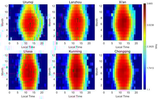
Figure 2. Monthly mean foE variation over the Tibetan Plateau and adjacent regions based on local time.

As shown in Figure 2, quantitative analysis reveals obvious spatiotemporal distribution patterns of the ionospheric E layer intensity over the Tibetan Plateau region. The foE values exhibit significant diurnal and seasonal variations, with the foE in the Tibetan Plateau region ranging from 1.1 to 3.665 MHz. The peak intensity consistently occurs at local noon. Five out of the six stations show the maximum value at 12:00 local time in July, while the peak at Urumqi is slightly later, appearing at 13:00 local time in June.

Due to the absence of solar radiation at night, the intensity of the regular E-layer weakens significantly or even disappears, so the detectable foE signals at night are smaller than those during the day. Low-latitude stations (Kunming, Chongqing) show higher data coverage in the early morning, which may be related to E-layer irregularities, and further in-depth studies will be conducted on this in the future. As can be seen from Figure 2, the occurrence frequency of the nocturnal E-layer demonstrates significant seasonal variation: it is markedly lower in summer but relatively higher in spring and autumn. This pattern is particularly pronounced at the Xi’an and Lhasa stations.

Normally, the E-layer gradually disappears after sunset due to the cessation of solar radiation and recombination processes. However, exceptional cases do exist. The nocturnal E-layer manifestation is termed “particle E-layer”, which exhibits both: characteristic E-layer morphology on ionograms (evidenced by parabolic trace curvature rather than horizontal linearity) and sporadic occurrence patterns akin to Es-layer behavior [29,30,31]. The prevailing hypothesis in contemporary aeronomy attributes the formation of particle E-layers to anomalous ionospheric disturbances. Seasonally, particle E-layers predominantly occur during spring and autumn (as evidenced in Figure 2), exhibiting a striking divergence from the summer-dominated occurrence of sporadic E layers, demonstrating conclusively that particle E-layers fall outside the taxonomic category of Es layers. The nocturnal E-layer phenomena documented in this study predominantly represent instances of particle E-layer.

3.2. Spatial Distribution of the Ionospheric E Layer over the Tibetan Plateau

To examine the spatial distribution characteristics of the ionospheric E layer over the Tibetan Plateau, this study utilizes foE observations from six ionosonde stations located within and around the plateau region.

To characterize the spatial distribution of foE intensity, we calculated the mean foE at local noon (12:00 LT) by averaging all available observations over the 11-year period (2013–2023). Noon time was selected because foE reaches its maximum value during this period due to peak solar radiation.

The Kriging interpolation method was adopted in this study to derive the regional annual mean value of foE distribution, as presented in Figure 3 [32,33].

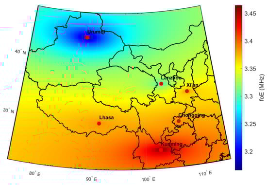
Figure 3. foE distribution over the Tibetan Plateau and surrounding area at noon.

Kriging is specifically designed to model such spatially correlated geophysical data by capturing the spatial structure through semivariograms, providing more accurate estimates than traditional methods such as inverse distance weighting. Second, the study area faces the challenge of sparse and irregular data distribution, with only six observation stations covering a large region. Kriging is well-suited for such conditions, as it offers reliable interpolation through an optimized weighting strategy that accounts for both spatial distance and correlation structure.

Figure 3 shows the annual mean spatial distribution of foE. The results show that foE values generally range between 3.2 and 3.45 MHz across the study area at noon, with higher values typically occurring in lower-latitude regions due to smaller solar zenith angles, which enhance solar irradiance and ionization rates. In particular, relatively low foE values are observed in the Xinjiang region (centered around Urumqi), followed by Lanzhou, whereas higher values are evident in lower-latitude stations such as Kunming and Lhasa. However, the foE distribution does not strictly conform to a latitudinal gradient. For instance, Lhasa exhibits significantly higher foE values than Chongqing, despite their similar latitudes. This discrepancy suggests that factors beyond latitude contribute to the spatial pattern of foE. Several mechanisms are likely involved in shaping this complexity, including the high-altitude effect—Lhasa’s elevation (~3650 m) greatly exceeds that of Chongqing (200–400 m), thereby reducing atmospheric attenuation and increasing ultraviolet radiation. The region’s unique atmospheric circulation and gravity wave activity may also modify the composition and density of the neutral atmosphere. Overall, the spatial distribution of foE over the Tibetan Plateau reflects a complex interplay among solar radiation, topographic elevation, geomagnetic conditions, and atmospheric dynamics, underscoring the scientific importance of ionospheric studies in this high-altitude region.

To further assess the quality and reliability of the spatial interpolation, this study applies geostatistical methods to perform a variogram analysis on the interpolated grid of the ionospheric E layer critical frequency (foE) over the Tibetan Plateau region. Variogram analysis is a fundamental geostatistical technique that quantifies spatial autocorrelation by measuring the variance between data points as a function of distance and direction. This method allows us to evaluate the spatial structure and continuity of the interpolated foE values, thereby providing insights into the reliability and accuracy of the kriging interpolation results [34].

As shown in Figure 4, the spatial distribution of the ionospheric E-layer critical frequency (foE) over the Tibetan Plateau is further evaluated using geostatistical analysis. The variogram of the interpolated foE field reveals a clear anisotropic spatial pattern, with the semi-variance in the north–south direction being nearly four times larger than that in the east–west direction. This indicates that the spatial variability of foE is much stronger in latitude than in longitude, consistent with the geographic orientation and topography of the Plateau. The smooth and continuous increase in the variogram curves suggests good spatial autocorrelation and stability of the interpolation, implying that the kriging-based spatial estimation is reliable under sparse station coverage. Moreover, the absence of abrupt fluctuations in the variogram further supports the robustness of the interpolation and demonstrates that kriging provides meaningful insight into the continuous spatial structure of the E-layer, which cannot be captured by the six discrete ionosonde observations alone.

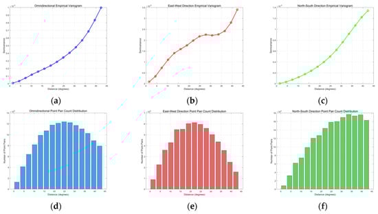
Figure 4. Variogram analysis of the foE interpolation network. (a) Omnidirectional empirical variogram. (b) Empirical variogram in the east−west direction. (c) Empirical variogram in the north−south direction. (d) Omnidirectional point pair count distribution. (e) Point pair count distribution in the east−west direction. (f) Point pair count distribution in the north−south direction.

3.3. Temporal Variation Characteristics of Ionospheric foE over the Tibetan Plateau

3.3.1. Diurnal Variation in Ionospheric foE

To further investigate the diurnal variation patterns of foE over the Tibetan Plateau, this study presents the average daily variation curves of ionospheric foE derived from six stations distributed across the plateau (see Figure 5 and Figure 6).

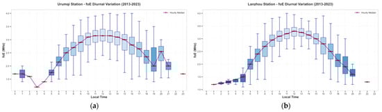
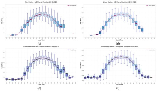
Figure 5. Diurnal Variation in foE at Six Ionosonde Stations Based on Local Time. (a) Urumqi diurnal foE value. (b) Lanzhou diurnal foE value. (c) Xi’an diurnal foE value. (d) Lahsa diurnal foE value. (e) Kunming diurnal foE value. (f) Chongqing diurnal foE value.

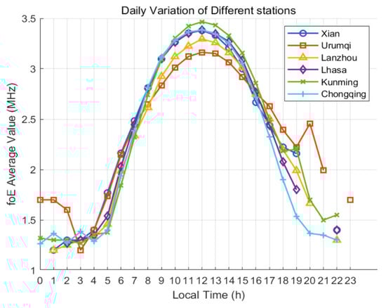
Figure 6. Comparative hourly mean diurnal variation in foE at six ionosonde stations based on local time.

Figure 5 depicts the mean diurnal variation in foE at the six observation stations. All stations exhibit a typical pattern characterized by elevated foE values during daytime hours (09:00–17:00 LT) and reduced values at night (22:00–06:00 LT), reflecting the modulation of E-layer electron density by solar radiation. During daytime, the boxplots shift upward, indicating a significant increase in electron density driven by intensified solar ionization. In contrast, nighttime boxplots are confined to a lower frequency range (1.4–1.8 MHz) and exhibit a narrower distribution, suggesting weakened ionization and greater stability of foE at lower levels. The most substantial foE fluctuations generally occur around sunrise and sunset, coinciding with rapid changes in solar zenith angle. Notably, the magnitude of diurnal foE variations varies considerably across the stations. Higher-latitude stations show more pronounced fluctuations, as indicated by wider boxplot spreads, whereas lower-latitude stations display relatively stable patterns. Urumqi demonstrates the highest degree of diurnal variability, characterized by broad daytime spreads and significantly lower foE values at night. In contrast, Kunming exhibits the smallest amplitude of change and maintains relatively elevated nighttime foE levels. These spatial differences underscore the critical role of solar zenith angle variation in regulating E-layer intensity across latitudes. Figure 6 presents the corresponding average diurnal variation curves for foE at the six stations, which align closely with the boxplot patterns described above, further confirming the dominant influence of solar-driven ionization on diurnal E-layer behavior.

To further investigate the diurnal variation characteristics of E-layer intensity over the Tibetan Plateau and its surrounding regions, Figure 7 displays the spatial distribution of mean ionospheric foE values during the daytime period (08:00–17:00) and the nighttime period (22:00–06:00 of the following day), respectively.

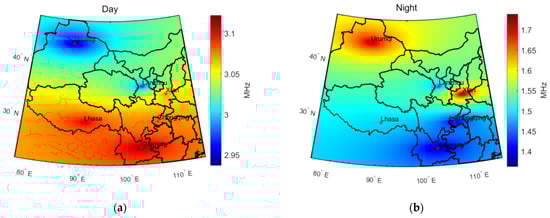
Figure 7. Spatial comparison of mean daytime and nighttime foE over the Tibetan Plateau region. (a) Daytime mean foE over the Tibetan Plateau region. (b) Nighttime mean foE over the Tibetan Plateau region.

The results show that during the daytime period (08:00–17:00), ionospheric foE values are generally higher than at night (22:00–06:00, next day), ranging between 2.95 and 3.1 MHz. At night, foE significantly decreases, with values distributed between 1.4 and 1.7 MHz. Spatially, Kunming exhibits the strongest E-layer intensity during the day, whereas Urumqi remains at the lowest level. Overall, foE demonstrates a decreasing trend from low to high latitudes during daytime, consistent with the theory that the E-layer intensity varies with solar radiation. Conversely, at night, foE shows an increasing trend from low to high latitudes, essentially opposite to the daytime distribution. Kunming, which has the highest daytime E-layer intensity, becomes one of the regions with the lowest intensity at night, while Urumqi shows the opposite behavior. This indicates a pronounced day-night asymmetry of the ionospheric E layer over the Tibetan Plateau and its surrounding areas, which is the most significant characteristic of E-layer variability in this region.

A further comparison of diurnal amplitude variation among the stations reveals that Kunming experiences the largest day-night variation in foE, followed by Chongqing, then Lhasa, Xi’an, Lanzhou, and Urumqi. This pronounced diurnal asymmetry suggests that, in addition to solar radiation as the primary controlling factor, local topographic influences also play a critical role in modulating E-layer intensity. In low-latitude, topographically complex areas such as Kunming and Chongqing, surface heating induces strong convective activity during the day, facilitating more efficient upward energy transport to E-layer altitudes and enhancing ionization, thus producing higher foE values. At night, with the cessation of solar radiation, convection rapidly weakens, leading to a swift decline in electron density and a notable reduction in E-layer activity. In contrast, Urumqi, located at higher latitude and at the edge of a basin surrounded by enclosed terrain, experiences a relatively stable atmosphere that inhibits the vertical propagation of surface thermal disturbances. Consequently, daytime E-layer enhancement is limited, and the E-layer maintains a degree of stability at night, resulting in smaller diurnal variation. Topography exerts a significant modulatory effect on the formation and maintenance of the ionospheric E-layer by influencing local thermal structures and atmospheric vertical disturbances. It should be noted that the phenomenon of significantly higher foE values at higher latitudes than at lower latitudes during nighttime may be related to convection induced by topography. However, this is currently only speculation, and it remains uncertain whether there are other more dominant controlling factors.

3.3.2. Seasonal Variation Characteristics

To further investigate the seasonal evolution of the ionospheric E layer over the Tibetan Plateau, Figure 8 and Figure 9 present radar charts illustrating the seasonal variations in the monthly mean foE values at six ionosonde stations: Urumqi, Lanzhou, Xi’an, Lhasa, Kunming, and Chongqing.

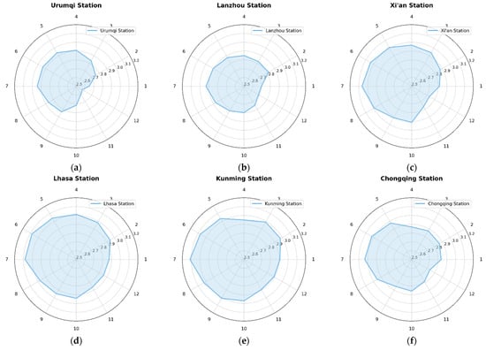
Figure 8. Seasonal variation in average foE at six ionosonde stations. (a) Urumqi (b) Lanzhou (c) Xi’an (d) Lhasa (e) Kunming (f) Chongqing.

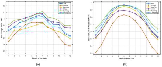
Figure 9. FoE over the Tibetan Plateau and the layout of cosine of the solar zenith angle. (a) Comparative monthly variation in mean foE at six ionosonde stations. (b) Monthly Average of cos(SZA) at Noon.

From Figure 8 and Figure 9, it can be observed that the monthly mean foE values of the ionospheric E layer at the six stations across the Tibetan Plateau and its surrounding regions exhibit a generally consistent annual variation pattern. Overall, all six stations show a peak during summer (June–August) and a trough in winter (November to February of the following year), presenting a typical “unimodal” annual variation structure. This seasonal trend aligns with the theoretical mechanism that the E-layer is primarily controlled by solar radiation: during summer, the solar zenith angle is smaller, leading to enhanced ionization and increased electron density in the E-layer, thus resulting in higher foE values, whereas in winter, weaker radiation leads to reduced ionization and lower foE values.

However, the seasonal variation in foE over the Tibetan Plateau and its surrounding regions is not entirely governed by changes in the solar zenith angle. As shown in Figure 8, the peak foE values at most stations occur in July rather than in June, when the solar zenith angle reaches its minimum. Additionally, at Kunming and Xi’an, the foE values in April are significantly lower than those in March, and at Chongqing and Xi’an, the values in October exceed those in September. This inconsistency between E-layer intensity and solar zenith angle variation represents another notable seasonal characteristic of the E-layer in the Tibetan Plateau and surrounding areas. Figure 8 further illustrates that this inconsistency is mainly observed in July (after the summer solstice), as well as in April and October (months following the equinoxes). The affected stations—Kunming, Chongqing, and Xi’an—are all located in regions with complex terrain. The peak foE values in July may be attributed to the highest surface temperatures during this period in the Tibetan Plateau and surrounding regions, which can trigger intense vertical motion in the troposphere. Through coupling mechanisms between the lower and upper atmosphere, energy is transferred to E-layer altitudes, thereby enhancing the 1 in the E region. The anomalous foE variations observed at Kunming, Chongqing, and Xi’an in April and October may also be related to the complex topographic structures in these regions.

To further investigate the long-term variation in the ionospheric E layer foE mean values over the Tibetan Plateau, Figure 10 presents the spatial distributions of mean foE during summer and winter, respectively.

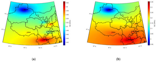
Figure 10. Comparison of mean foE values between summer and winter over the Tibetan Plateau at noon (a) Summer mean foE over the Tibetan Plateau region. (b) Winter mean foE over the Tibetan Plateau region.

As shown in Figure 10, foE values in winter are generally lower than those in summer. Over the Tibetan Plateau and its surrounding regions, the winter time mean foE values at noon range from 2.95 to 3.35 MHz, while the summertime values lie between 3.4 and 3.6 MHz. On average, the mean foE in summer is approximately 10% higher than in winter. This seasonal difference is consistent with the fundamental physical mechanism that the ionospheric E layer is primarily driven by solar ultraviolet radiation. In summer, the solar zenith angle is smaller and solar radiation is stronger, which enhances ionization and increases the electron density in the E-layer, thereby raising foE values. In contrast, during winter, shorter daylight hours and weaker solar radiation reduce ionization efficiency, leading to lower electron densities and thus lower foE values.

3.3.3. Variation with the Solar Cycle

The electron density of the ionospheric E region is mainly governed by solar radiation, and consequently, the intensity of the E-layer is markedly affected by solar activity.

To conduct an in-depth study of the solar cycle variation characteristics of the ionospheric E-layer intensity over the Tibetan Plateau and its surrounding regions, Figure 11 and Figure 12 utilize data from one solar cycle spanning 2013 to 2023. The monthly mean foE measurements from six ionosonde stations—Urumqi, Lanzhou, Xi’an, Lhasa, Kunming, and Chongqing—are plotted alongside the monthly mean sunspot numbers to analyze the correlation between the E-layer intensity and solar activity in this region.

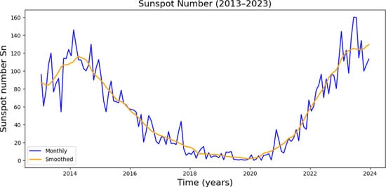
Figure 11. Variation in sunspot numbers.

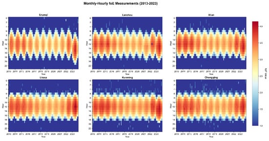
Figure 12. Solar cycle variations in ionospheric foE in the Tibetan Plateau region.

A joint examination of Figure 11 and Figure 12 reveals distinct solar cycle variations in foE over the Tibetan Plateau and surrounding regions. During solar minimum years (2018–2020), the ionospheric E layer intensity was significantly lower compared to that in solar maximum years (2013–2015), suggesting a strong positive correlation between E-layer intensity and solar activity in this region. To further investigate the correlation between E intensity and sunspot numbers, the Pearson correlation coefficient was used. The monthly median value of E intensity and the monthly mean value of sunspot numbers in the corresponding period were used, respectively. It is calculated by dividing the covariance of two variables by their standard deviations, and its formula is as follows:

$$COR(X,Y)={\displaystyle \frac{cov(X,Y)}{{\mathsf{\sigma }}_X{\mathsf{\sigma }}_Y}}={\displaystyle \frac{E\left(XY\right)-E\left(X\right)E\left(Y\right)}{\sqrt{E\left(X^2\right)-E\left(Y^2\right)}\sqrt{E\left(Y^2\right)-E\left({YX}^2\right)}}}$$

(3)

where $X$ is the value of the monthly median value of $E$ intensity for a certain region, and $Y$ represents the monthly mean value of sunspot numbers in the corresponding period and region. The correlation coefficient between $E$ intensity and sunspot numbers for 6 stations in Tibetan Plateau and surrounding areas is shown in Table 2:

Table 2. Correlation between E intensity and sunspot numbers in Tibetan Plateau and surrounding areas.

Index	Station Name	Correlation Coefficient
1	Chongqing	0.553
2	Lanzhou	0.572
3	Lhasa	0.675
4	Urumchi	0.581
5	Kunming	0.621
6	Xi’an	0.597

The correlation coefficient between E intensity and sunspot numbers for 6 stations is analyzed and shown in Table 2 after interpolation in Tibetan Plateau and surrounding areas. It is shown that there is a medium correlation between E intensity and the sunspot numbers, and the correlation coefficient generally ranges from 0.55 to 0.67, with the mean correlation coefficient being 0.6, where the maximum value is 0.675 in Lhasa, and the minimum value is 0.553 in Chongqing. According to the correlation theory, it is generally considered that the correlation coefficient of 0–0.3 is weak correlation, the correlation coefficient of 0.3–0.7 is medium correlation, and the correlation coefficient of 0.7–1 is strong correlation [35,36]. Therefore, through the analysis on correlation, it can be concluded that the correlation coefficient between E intensity and sunspot numbers is 0.6, which is a medium correlation.

Solar activity enhances the ionization of the ionospheric E layer by increasing ultraviolet and X-ray radiation, which in turn raises electron density and elevates the critical frequency (foE). During solar maxima, elevated sunspot numbers correspond to stronger solar radiation and thus more intense ionization, resulting in higher foE values. In contrast, during solar minima, the reduced solar output leads to diminished ionization and electron density, thereby lowering foE levels.

To further investigate the modulation effect of solar activity on the ionospheric E layer, this study calculated the interannual relative variograms of foE (critical frequency of the ionospheric E layer) data. The relative variogram, an important tool in geostatistics for analyzing the variation characteristics of spatial data, is a derivative form of the traditional variogram. Its core value lies in eliminating the interference of data magnitude differences on spatial correlation analysis through standardized processing. Compared with the traditional variogram, it focuses more on capturing the relative variability of data, which not only facilitates the comparison of spatial correlations between different regions and variables but also more sensitively reflects the relative fluctuation degree of data in space. The Figure 13 shows the results of the relative variograms of foE in different years.

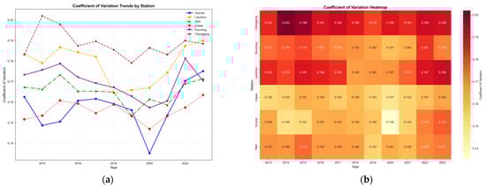
Figure 13. Data variation among different stations. (a) Six-station coefficient of variation temporal evolution. (b) Station-year coefficient of variation heatmap.

Results from the spatiotemporal analysis based on the coefficient of variation reveal distinct patterns of temporal synchrony and spatial heterogeneity in the foE variability across the six ionosonde stations.

Temporally, all stations exhibited the lowest variability around 2020, followed by a gradual rebound from 2021 to 2023. This trend suggests the influence of common environmental or observational drivers—primarily the overarching modulation of ionospheric E layer intensity by solar activity. Spatially, the stations show significant stratification in variability. The Chongqing station consistently maintained a high coefficient of variation across both high and low solar activity periods, indicating relatively poor data stability. This suggests that, in addition to solar activity, other regional factors may exert substantial influence. In contrast, the Urumqi and Lanzhou stations exhibited fluctuations in variability that closely tracked the solar cycle, implying a stronger regulatory effect of solar activity. The Lhasa station had the lowest coefficient of variation (0.13–0.17), reflecting the most stable data quality among all stations. The remaining stations demonstrated moderate levels of variability.

The heatmap visualization further supports these spatiotemporal patterns. Overall, ionospheric E layer stability is closely tied to solar activity: stability tends to decrease during periods of high solar activity and improve during solar minima. The observed spatial heterogeneity reflects region-specific modulation of the E-layer by local environmental conditions.

4. Discussion

The Tibetan Plateau and its surrounding areas primarily generate gravity waves through two mechanisms: dynamic uplift/blocking and thermal forcing [37]. These gravity waves propagate upward into the stratosphere, mesosphere, and even the thermosphere. Upon breaking, they transfer momentum to the background atmosphere, significantly influencing atmospheric circulation and material distribution at these altitudes. Chen et al. [38] successfully observed gravity wave phenomena within intermediate descending layers (IDLs) during the solar eclipse on 21 June 2020. By coordinating observations from five ionosondes, they proposed an explanation for the modulation of the E-layer by gravity waves.

Gravity waves potentially excited by the Tibetan Plateau’s topography may propagate to E-layer altitudes, manifesting as short-period vertical oscillations. Gravity waves modulate foE by influencing wind shear. When gravity waves propagate into unstable regions, they are more prone to breaking and dissipate their energy in the form of turbulence. According to the law of energy conservation, as atmospheric density decreases with increasing altitude, the amplitude of gravity waves gradually increases. When gravity waves traverse the mesopause, their wave amplitude, wave-induced temperature changes, and wind shear all reach extremely high values, causing the gravity waves to become unstable and more likely to break down into turbulence. This process leads to the deposition of the momentum flux carried by the gravity waves into the mean flow, thereby accelerating or decelerating the mean wind speed, and even potentially reversing its direction [39,40].

The observed diurnal and seasonal asymmetries in the intensity of the regular E-layer over the Tibetan Plateau and its surrounding areas may result from variations in the dominant controlling factors of foE across different periods. During daytime, the electron density of the E-layer is primarily governed by solar radiation, showing significant latitudinal dependence. However, when solar radiation weakens at night or during winter and spring seasons, its controlling effect diminishes, allowing the influence of factors such as gravity waves generated by complex topography to become more pronounced. This leads to enhanced irregular variability in E-layer characteristics.

5. Conclusions

The ionospheric E layer over the Tibetan Plateau and its surrounding regions predominantly manifests during daytime, with peak intensity near local noon and the weakest intensity in the early morning hours. The E-layer intensity exhibits pronounced seasonal variations, reaching its maximum in summer and minimum in winter. Monthly mean foE values across the region range from 1.3 MHz to 4.2 MHz, displaying a latitudinal zonal distribution pattern, where intensity gradually decreases toward higher latitudes.

Regarding diurnal variation, maximum foE values typically occur at 12:00 local time, while minimum values are observed around 03:00. Daytime E-layer intensity is significantly greater than nighttime levels. Seasonally, peak foE values generally occur in July, with the lowest in December, and the strongest month’s foE exceeding that of the weakest by approximately 20–30%.

Furthermore, the E-layer intensity shows a clear positive correlation with solar activity, particularly during summer in solar maximum years, when the E-layer is markedly stronger than during solar minimum years.

Beyond the typical E-layer variation patterns seen in mid- and low-latitude regions, the ionospheric E layer over the Tibetan Plateau exhibits unique spatiotemporal distribution features. Notably, a pronounced day–night asymmetry in E-layer intensity exists across the region. Additionally, some local stations display E-layer variation patterns deviating from expectations based solely on solar zenith angle changes. These distinctive features are likely related to the region’s complex topography, which fosters intricate coupling mechanisms between the lower and upper atmosphere.

Spatiotemporal analysis based on the coefficient of variation further reveals distinct temporal synchrony and spatial heterogeneity in data variability among the six stations. Temporally, all stations showed minimum variability around 2020, followed by a recovery phase from 2021 to 2023, reflecting the overarching influence of solar activity. Spatially, variability is stratified: Chongqing exhibits persistently high variability (indicating poor stability) influenced by factors beyond solar activity; Urumqi and Lanzhou demonstrate stronger variability modulated by solar activity; Lhasa maintains the lowest variability (0.13–0.17), indicating relatively stable data quality; other stations show moderate variability. Overall, station data stability closely correlates with solar activity—being poorer during high-activity years and better during low-activity years—while spatial heterogeneity reflects differential modulation by regional environmental factors.

References

- Liu, V.C. On ionospheric aerodynamics. Prog. Aerosp. Sci. 1975, 16, 273–297. [Google Scholar] [CrossRef][Green Version]
- Lindinger, W.; Fehsenfeld, F.C.; Schmeltekopf, A.L.; Ferguson, E.E. Temperature dependence of some ionospheric ion–neutral reactions from 300°–900 K°. J. Geophys. Res. 1974, 79, 4753–4756. [Google Scholar] [CrossRef]
- Titheridge, J.E. Model results for the daytime ionospheric E and valley regions. J. Atmos. Sol.-Terr. Phys. 2003, 65, 129–137. [Google Scholar] [CrossRef]
- Wu, S.Y. Ionosphere and radio wave communication. Daxue Wuli 1998, 11, 28–30. [Google Scholar]
- Davies, K. Ionospheric Radio; Peter Peregrinus Ltd.: London, UK, 1990. [Google Scholar]
- Budden, K.G. Radio Waves in the Ionosphere; Cambridge University Press: Cambridge, UK, 1961. [Google Scholar]
- Liu, T.; Wang, S.; Liu, S.; Zhang, R.; Liu, C. Influence of the ionospheric E layer on the characteristics of satellite-to-ground quantum key distribution. J. Beijing Univ. Posts Telecommun. 2023, 46, 35–40. [Google Scholar]
- Chapman, S. The absorption and dissociative or ionizing effect of monochromatic radiation in an atmosphere on a rotating earth. Proc. Phys. Soc. 1931, 43, 26–45. [Google Scholar] [CrossRef]
- Hoque, M.M.; Jakowski, N. Ionospheric propagation effects on GNSS signals and new correction approaches. GPS Solut. 2012, 16, 247–258. [Google Scholar]
- Wang, X.L.; Huang, Z.R. Calculation of the electron density profile of the mid-latitude E-layer critical frequency and lower ionosphere. Chin. J. Space Sci. 1985, 5, 199–208. [Google Scholar] [CrossRef]
- Titheridge, J.E. Modelling the peak of the ionospheric E-layer. J. Atmos. Sol.-Terr. Phys. 2000, 62, 93–114. [Google Scholar] [CrossRef]
- Bilitza, D.; Altadill, D.; Zhang, Y.; Mertens, C.J.; McKinnell, L.A.; Reinisch, B.W.; Fuller-Rowell, T.J. The International Reference Ionosphere Model: A review and description of an ionospheric benchmark. Rev. Geophys. 2022, 60, e2022RG000792. [Google Scholar] [CrossRef]
- Peng, Y.; Scales, W.A.; Hartinger, M.D.; Xu, Z.; Coyle, S. Characterization of multi-scale ionospheric irregularities using ground-based and space-based GNSS observations. Satell. Navig. 2021, 2, 14. [Google Scholar] [CrossRef]
- Sun, Y.-Y. GNSS brings us back on the ground from ionosphere. Geosci. Lett. 2019, 6, 14. [Google Scholar] [CrossRef]
- Angling, M.J.; Nogués-Correig, O.; Nguyen, V.; Vetra-Carvalho, S.; Bocquet, F.-X.; Nordstrom, K.; Melville, S.E.; Savastano, G.; Mohanty, S.; Masters, D. Sensing the ionosphere with the Spire radio occultation constellation. J. Space Weather Space Clim. 2021, 11, 56. [Google Scholar] [CrossRef]
- De Franceschi, G.; Spogli, L.; Alfonsi, L.; Romano, V.; Cesaroni, C.; Hunstad, I. The ionospheric irregularities climatology over Svalbard from solar cycle 23. Sci. Rep. 2019, 9, 9232. [Google Scholar] [CrossRef] [PubMed]
- Reinisch, B.W.; Galkin, I.A.; Khmyrov, G.M.; Kozlov, A.V.; Bibl, K.; Lisysyan, I.A.; Cheney, G.P.; Huang, X.; Kitrosser, D.F.; Paznukhov, V.V.; et al. New Digisonde for research and monitoring applications. Radio Sci. 2009, 44, RS0A24. [Google Scholar] [CrossRef]
- Reinisch, B.W.; Galkin, I.A.; Belehaki, A.; Paznukhov, V.; Huang, X.; Altadill, D.; Buresova, D.; Mielich, J.; Verhulst, T.; Stankov, S.; et al. Pilot ionosonde network for identification of traveling ionospheric disturbances. Radio Sci. 2018, 53, 365–378. [Google Scholar] [CrossRef]
- Arras, C.; Jacobi, C.; Wickert, J. Semidiurnal tidal signature in sporadic E occurrence rates derived from GPS radio occultation measurements at higher midlatitudes. Ann. Geophys. 2009, 27, 2555–2563. [Google Scholar] [CrossRef]
- Liu, D. Study on the Characteristics of Es over the Tibetan Plateau and Surrounding Regions. Ph.D. Thesis, China Academy of Electronics and Information Technology, Beijing, China, 2023. [Google Scholar]
- Yu, Y.; Wan, W.; Xiong, B.; Ren, Z.; Zhao, B.; Zhang, Y.; Ning, B.; Liu, L. Modeling Chinese ionospheric layer parameters based on EOF analysis. Space Weather 2015, 13, 339–355. [Google Scholar] [CrossRef]
- Bremer, J. Long-term trends in the ionospheric E and F1 regions. Ann. Geophys. 2008, 26, 1189–1197. [Google Scholar] [CrossRef]
- Tan, H.; Wan, W.X.; Lei, J.H.; Liu, L.-B.; Ning, B.-Q. A theoretical model for the mid-latitude ionospheric E layer. Chin. J. Geophys. 2005, 48, 243–251. [Google Scholar] [CrossRef]
- Yue, X.A.; Wan, W.X.; Liu, L.B.; Ning, B. An empirical model of ionospheric foE over Wuhan. Earth Planets Space 2006, 58, 323–330. [Google Scholar] [CrossRef]
- Huang, Z. Characterization of ionospheric E-layer scintillation index along the longitude 120°E using COSMIC during 2007–2013. Chin. J. Geophys. 2017, 60, 480–488. [Google Scholar]
- Sivakandan, M.; Mielich, J.; Renkwitz, T.; Chau, J.L.; Jaen, J.; Laštovička, J. Long-term variations and residual trends in the E, F, and sporadic E (Es) layer over Juliusruh, Europe. J. Geophys. Res. Space Phys. 2023, 128, e2022JA031097. [Google Scholar] [CrossRef]
- Zhu, M.; Xu, T.; Hu, Y.; Wu, J.; Ge, S. Construction of a physical model for the low ionosphere at low and middle latitudes. J. Rad. Sci. 2019, 34, 196–202. [Google Scholar]
- Liu, R.; Quan, K.; Dai, K.; Luo, F.; Sun, X.; Li, Z. Correction method for using the International Reference Ionosphere over China. Chin. J. Geophys. 1994, 37, 422–432. [Google Scholar]
- Chen, B.; Liu, Y.; Feng, J.; Zhang, Y.; Zhou, Y.; Zhou, C.; Zhao, Z. High-resolution observation of ionospheric E-layer irregularities using multi-frequency range imaging technology. Remote Sens. 2023, 15, 285. [Google Scholar] [CrossRef]
- Patra, A.K.; Sripathi, S.; Sivakumar, V.; Rao, P.B. Statistical characteristics of VHF radar observations of low-latitude E-region field-aligned irregularities over Gadanki. J. Atmos. Sol.-Terr. Phys. 2004, 66, 1615–1626. [Google Scholar] [CrossRef]
- Bilitza, D.; Altadill, D.; Zhang, Y.L.; Mertens, C.; Truhlik, V.; Richards, P. The International Reference Ionosphere 2012—A model of international collaboration. J. Space Weather Space Clim. 2014, 4, A07. [Google Scholar] [CrossRef]
- Stanislawska, I.; Juchnikowski, G.; Cander, L.R. The Kriging method of ionospheric parameter f0F2 instantaneous mapping. Ann. Geophys. 1996, 39, 845–852. [Google Scholar] [CrossRef]
- Liu, Y.; Yu, Q.; Shi, Y.; Yang, C.; Wang, J. A reconstruction method for ionospheric foF2 spatial mapping over Australia. Atmosphere 2023, 14, 1399. [Google Scholar] [CrossRef]
- Oliver, M.A.; Webster, R. Basic Steps in Geostatistics: The Variogram and Kriging; Springer Briefs in Agriculture; Springer International Publishing: Cham, Switzerland; Berlin/Heidelberg, Germany; New York, NY, USA; Dordrecht, The Netherlands; London, UK, 2015. [Google Scholar]
- Feng, J.; Zhao, H.S.; Liu, Y.; Guo, L.-X.; Wu, J.; Xu, Z.-W.; Tang, H.-Y.; Li, N.; Ding, Z.-H. Characteristics of Sporadic E layer in Japan based on multi-station detection Study on characteristics of Es in East Asia. Opt. Express 2025, 33, 35560–35575. [Google Scholar] [CrossRef] [PubMed]
- Ge, S.; Li, H.; Xu, T.; Zhu, M.; Wang, M.; Meng, L.; Ullah, S.; Rauf, A. Characteristics of the layered polar mesosphere summer echoes occurrence ratio observed by EISCAT VHF 224 MHz radar. Ann. Geophys. 2019, 37, 417–427. [Google Scholar] [CrossRef]
- Wei, D.; Tian, W.S.; Chen, Z.Y.; Zhahg, J.K.; Xu, P.P.; Huang, Q.; Han, Y.Y.; Zhang, J. Upward transport of air mass during a generation of orographic waves in the UTLS over the Tibetan Plateau. Chin. J. Geophys. 2016, 59, 791–802. (In Chinese) [Google Scholar] [CrossRef]
- Chen, G.; Cai, X.; Zhang, S.; Gong, W.; Yang, G.; Wang, Y.; Hu, L.; Zhong, D.; Li, Y.; Xu, Y.; et al. Intermediate descending layers emerged simultaneously in five different locations during the solar eclipse on 21 June 2020. J. Geophys. Res. Space Phys. 2024, 129, e2023JA032340. [Google Scholar] [CrossRef]
- Liu, X.; Xu, J.; Liu, H.L.; Yue, J.; Yuan, W. Simulations of large winds and wind shears induced by gravity wave breaking in the mesosphere and lower thermosphere (MLT)region. Ann. Geophys. 2014, 32, 543–552. [Google Scholar] [CrossRef]
- Li, T.; She, C.-Y.; Liu, H.-L.; Yue, J.; Nakamura, T.; Krueger, D.A.; Wu, Q.; Dou, X.; Wang, S. Observation of local tidal variability and instability, along with dissipation of diurnal tidal harmonics in the mesopause region over Fort Collins, Colorado(41°N,105°W). J. Geophys. Res. 2009, 114, D06106. [Google Scholar]
Disclaimer/Publisher’s Note: The statements, opinions and data contained in all publications are solely those of the individual author(s) and contributor(s) and not of MDPI and/or the editor(s). MDPI and/or the editor(s) disclaim responsibility for any injury to people or property resulting from any ideas, methods, instructions or products referred to in the content. |
© 2025 by the authors. Licensee MDPI, Basel, Switzerland. This article is an open access article distributed under the terms and conditions of the Creative Commons Attribution (CC BY) license (https://creativecommons.org/licenses/by/4.0/).